

Generalized linear mixed models (GLMMs) offer a general framework for the analysis of multisite intervention studies with flexible models that reflect important features of the observed data, and accommodate the analysis of outcomes that are binary (eg, patient infection, yes/no), count (eg, infection counts per day), continuous (eg, length of stay in hospital) or skewed (eg, costs).
This article provides an introduction to GLMMs for a broad audience of professionals in infection control and hospital epidemiology. We review approaches for model fitting and assessment using current methods available in R, and we provide recommendations for summarizing model inference to address common research questions in infection control studies. Approaches are demonstrated using a real example from a study of examining a change in hospital cleaning policy. Links to data and R code are provided.
Infection control studies often collect data over time to test whether a new policy or practice was associated with a change in infection rates or surrogate outcome. Such designs commonly use data that are collected (1) before and after the policy change; (2) at the same sites over time, such as wards or hospitals; and/or (3) at a common time frequency, such as daily or weekly. This study design has several different names, including a pre–post or before-and-after study, change-point study, or interrupted time series. They are sometimes called “quasi-experimental,” studies, which identifies them as including a nonrandomized experiment as opposed to a controlled experiment in which study sites and/or individuals are randomly allocated to receiving the intervention or not.Reference Harris, Bradham, Baumgarten, Zuckerman, Fink and Perencevich1 Randomization is an ideal design because it wipes out potential confounding, but well-executed quasi-experimental studies can still provide valuable insights into the effects of a policy change. Previous papers have reviewed the main types of quasi-experimental designs,Reference Harris, Bradham, Baumgarten, Zuckerman, Fink and Perencevich1 and a useful book on quasi-experimental designs is available for those seeking detail.Reference Shadish, Cook and Campbell2
Methods for analyzing intervention studies in infection control have included group comparisons, regression, and time series methods.Reference Shardell, Harris, El-Kamary, Furuno, Miller and Perencevich3, Reference Pierce, Lessler and Milstone4 These methods are best suited to analyzing data collected from a single site. Multisite studies introduce new features into the data that may require different methods for testing the overall impact of an intervention. Examples of these features include differences in the intervention timing; baseline differences between sites that are unrelated to the policy change being evaluated; and the presence of clustering in the data from collecting multiple results per site.
In this article, we examine the use of generalized linear mixed models (GLMMs) for the analysis of multisite intervention studies. Our aim is to provide guidance on their applied use by researchers, from defining and fitting potential models to model assessment and presentation of findings. Concepts are demonstrated using data from a study evaluating the impact of an environmental cleaning bundle.
Methods
Our case study was taken from a stepped-wedged randomized trial of a cleaning bundle in Australian hospitals called the REACH study (Researching Effective Approaches to Cleaning in Hospitals).Reference Hall, Farrington and Mitchell5, Reference Mitchell, Hall and White6 A “bundle” is a combination of interventions, and for REACH the bundle included frequency of cleaning, cleaning techniques and auditing strategies, and environmental cleaning staff training.
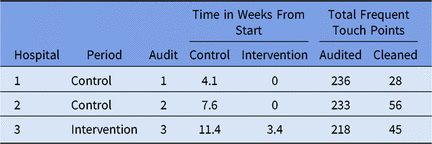
We examined the cleaning thoroughness of frequent touch points (FTPs), which was assessed using monthly cleaning audits. At the start of an audit, invisible gel dots were applied to 9–16 randomly selected FTPs in multiple patient cubicles and bathrooms. Following cleaning, the sites were checked by the site team using an ultraviolet light to determine whether the dot had been completely removed. Example data are shown in Table 1.
Three Rows of Example Data From the REACH Trial

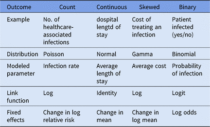
GLMM Specification for Different Outcomes Collected in Infection Control Studies

We completed 2 audits in each hospital during an 8-week control period. The cleaning bundle was then implemented, and audits were completed every 4 weeks until the end of the study.
A total of 11 hospitals received the cleaning bundle at randomly allocated times. Data from the 2 control audits and up to 10 intervention audits were included in the analysis. Data were analyzed to test whether cleaning performance improved after the intervention was introduced.
Common data features
When data are repeatedly collected over time, the following 3 features commonly occur. These features can bias our understanding of the intervention and should be controlled for using study design or statistical control.
1. Temporal patterns. The outcomes of interest may change slowly over time, for example, because of an ageing population or gradual improvements in clinical practice.
2. Seasonal patterns. Many infections have a seasonal pattern including surgical site infections,Reference Anthony, Peterson, Polgreen, Sewell and Polgreen7 Staphylococcus aureus,Reference Leekha, Diekema and Perencevich8 and Clostridium difficile.Reference Furuya-Kanamori, McKenzie and Yakob9 For example, an intervention that is introduced in every hospital just before winter runs the risk of wrongly ascribing the known winter peak in some infections to the policy change. Having at least 1 year of data before this change means a typical seasonal pattern can be estimated.
3. Other confounders. Other changes occurring in the intervention phase could lead to large changes in the outcome that might then appear to be associated with the policy change. Examples of changes unrelated to a study are a new drug becoming widely available and a pandemic.
Pre-existing trends
A common error when analyzing pre–post studies is to overlook trends that were already present in the preintervention period. For example, a pre–post study analyzed rates of methicillin-resistant Staphylococcus aureus bacteremia before and after a hand hygiene intervention.Reference Grayson, Jarvie and Martin10 In this study, the authors assumed that infection rates per 100 patient days were constant in the preintervention period. Estimating the change over time for the intervention gave a reduction of −0.018 per month (P < .001). However, infection rates appeared to be already declining before the intervention, possibly due to other factors. After adding a linear trend, the reduction in infections associated with the intervention more than halved to −0.007 per month (P = .31), giving much weaker evidence against the null hypothesis of no change in infection rates.
Correlated data
Generally, pre–post data should not be analyzed using a simple group comparison, for example, using a 2-sample t test for a continuous outcome. This is because the data may be positively correlated over time. This breaks the assumption of independent observations and may yield misleading results.
Collecting repeated data from the same sites means the data will likely be positively correlated because we expect results from the same site to be somewhat similar. For example, a hospital may have relatively high infection rates because of a challenging case mix of patients. Because our focus was on the change due to the intervention or policy change, we were disinterested in these common differences between sites, and therefore they were removed.
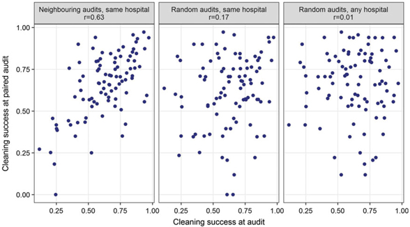
Figure 1 provides examples of correlation by site and time for our case study. We observed a clearly positive correlation in cleaning outcomes for neighboring audits at the same hospital with a Pearson correlation of 0.63. Randomly paired audits from the same hospital also showed some positive correlation (r = 0.17), likely caused by fixed within-hospital characteristics. In contrast, the correlation was almost zero (r = 0.01) for comparisons of 2 audits from any hospital at any time.
Scatterplot of the proportion of successfully cleaned FTPs for different pairings of cleaning audits.

Retrospective and prospective study designs
A retrospective assessment of a policy change would examine already collected data before and after the change, using routinely collected outcomes such as infection rates and length of hospital stay. In contrast, prospective designs are started before the policy change is implemented. The key advantage is that additional data can be collected that are not routinely available, for example, staff surveys before and after the change, or the cleaning audits in the REACH study.
Intervention timing
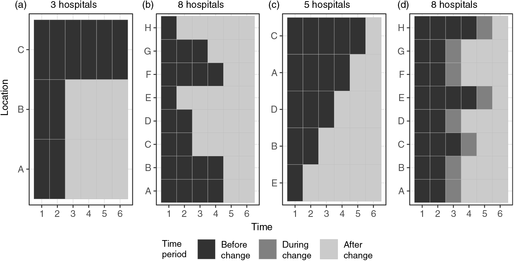
Figure 2 shows timings for 4 examples of multisite study designs. Some sites can be randomized to never receive the intervention (Fig. 2a), which provides a control site as a baseline for accounting for trends and other confounders. A potential downside to including a control site is that it may be difficult to recruit sites for a prospective study because at least 1 site will miss out on benefitting from the intervention. For a retrospective design with a control site, we need to understand why a site did not experience the policy change because selection bias may be present. For example, a site did not implement the change because they had very low infection rates or already had the policy in place.
Example study designs for a pre–post study: (a) design with a control site; (b) all sites experience the change with varying change-over time; (c) a stepped wedge design; (d) all sites experience the change with varying change-over times and a transition period. Note. Blue = before change, orange = during change, pink = after change.

Researchers may have little control over the timing of the intervention, which may be determined by policy makers or hospital executives (eg, Fig. 2b). In a stepped-wedge design (Fig. 2c), intervention timings are randomized by site, so the change will occur in some sites and not in others. Differing change times make for a stronger study design because randomization reduces correlation with other changes over time and the policy change of interest, thereby reducing confounding. In cases in which a lag occurs between implementing an intervention and its effect, an additional learning period can be added (Fig. 2d).
Generalized linear mixed models
We now describe how GLMMs can accommodate these features when analyzing data from multisite intervention studies. The main stages of GLMM specification are described using examples from infection control and the case study from the first section of text.
Choosing the outcome distribution
GLMMs offer a general framework for modeling binary, continuous, and count outcomes.Reference Stroup11 This flexibility comes from the ability to choose different probability distributions depending on the outcome, for example, infection counts or individual patient outcomes. Available distributions for GLMMs include the binomial distribution for binary data, the normal and gamma distributions for continuous data, and the Poisson distribution for count data. Examples of each distribution for common infection control outcomes are provided in Table 2.
Different outcome distributions will determine how changes due to the intervention and other factors are modeled. For example, data collected on number of healthcare-associated infections before and after a hand hygiene intervention can be modeled using a Poisson distribution where the intervention is associated with changes in infection rates.Reference Barnett, Page and Campbell12 For studies involving continuous outcomes, such as patient length of stay, choosing a normal distribution will model changes in average length of stay.Reference Graves, Weinhold and Tong13
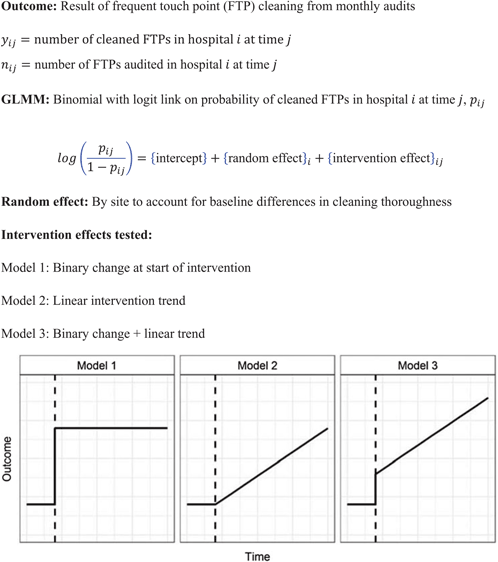
Our cleaning data were modeled using a binomial GLMM in which the outcome was the number of cleaned FTPs per the total number audited (Figure 3). Subsequent modeling, therefore, focused on the impact of the cleaning bundle on the probability of cleaned FTPs.
GLMM Specification for Case Study

Defining model effects
GLMMs use different types of effects for describing relationships between study variables and the outcome of interest, and for accounting for correlation among related observations. These effects are specified in the same way as a regression equation (Eq. 1):
 $$g\left( {\{ expected{\rm{ }}outcome\} } \right) = \left\{ {fixed{\rm{ }}effect\left( s \right)} \right\} + \left\{ {random{\rm{ }}effect\left( s \right)} \right\} + \left\{ {offset} \right\}$$
In a fixed effects model, the impact of the intervention and other study variables (eg, season, ward versus ICU) on the expected outcome is modeled. These models can also be used to account for outcome trends unrelated to the intervention. This is common in ‘interrupted time series’ designs in which time is included as a fixed effect, for example, in antimicrobial use before and after introducing additional antibiotic stewardship measures.Reference Taggart, Leung, Muller, Matukas and Daneman14
GLMMs differ from regression models using random effects to account for how data are collected under a study design. The role of random effects in multisite studies is 2-fold. First, for the designs in Figure 2, including a site-specific random effect effectively groups observations belonging to the same site. In doing so, we account for expected correlation between these observations (eg, see Fig. 1). Second, random effects account for between-site differences that are unrelated to intervention effectiveness, for example, baseline differences in cleaning thoroughness prior to the REACH bundle. By removing these differences, the estimated intervention effect represents the expected within-site change in the outcome of interest. This is important if modeling results are to be generalized, that is, if study sites are representative of the wider population. Examples of random effects for explaining other sources of variation are provided in the Supplementary Material online.
For count data, differences in site population sizes should be accounted for by specifying a model offset. For example, when modeling infection counts, differences in hospital size will inevitably create differences in infection counts between hospitals. Including hospital bed days as an offset will ensure that rates are modeled on a common scale (eg, infection rate per 10,000 bed days).Reference Mitchell, Hall and White6, Reference Barnett, Page and Campbell12
We tested 3 different intervention effects for describing the impact of the REACH bundle on cleaning thoroughness (Figure 3). Models that included temporal trends used audit times in weeks since the start of each hospital’s intervention phase. Changes over time were scaled by a factor of 10 to transform the trend to a more practically meaningful change (per 10 weeks).
Link function
Linear models assume that study variables share linear relationships with the outcome of interest and that residuals are normally distributed. These assumptions are inappropriate for outcomes modeled by nonnormal distributions. In some cases outcomes can be transformed to satisfy these assumptions; however, modeling results are difficult to interpret.
GLMMs resolve this issue by specifying a link function that connects the expected outcome with model effects. The form of the link function, g(·) in Equation (1), depends on the chosen outcome distribution. For infection counts modeled using the Poisson distribution, the log link function is used; fixed effects therefore summarize changes in each variable on the log relative risk of infection. For our binomial GLMM, using a logit link function means that effect of the bundle on cleaned FTPs is modeled on the log odds scale.
Model Fitting And Assessment
Software
GLMMs are available in many statistical software packages, including Stata (meglm), SAS (proc glimmix), and SPSS (GENLINMIXED). In R, the lme4 package (version 1.1-18-1)Reference Bates, Mächler, Bolker and Walker15 implements several likelihood-based methods for GLMM estimation and is compatible with other R packages for model assessment. Data and R code used in this article are available at https://github.com/nicolemwhite/ICHE_analysis.
Bayesian GLMMs are available in a number of software packages, including WinBUGS,Reference Sturtz, Ligges and Gelman16 JAGS,Reference Depaoli, Clifton and Cobb17 Greta,Reference Golding18 and R packages including MCMCglmmReference Hadfield19 and INLA.Reference Martins, Simpson, Lindgren and Rue20 Bayesian approaches differ from traditional likelihood methods by modeling uncertainty in both the data and unknown parameters, the latter requiring additional specification of prior distributions for each parameter in the model. In our experience, likelihood and Bayesian approaches for GLMMs yield similar results, except in cases where prior information may aide model estimation (eg, small sample sizes). When using Bayesian approaches, we recommend trying different prior distributions as part of model assessment because different choices may influence estimated model effects.Reference Lunn, Jackson, Best, Spiegelhalter and Thomas21 A review of Bayesian approaches to GLMMs is available elsewhere.Reference Fong, Rue and Wakefield22
Model selection
Information criteria are recommended as a parsimonious approach for choosing between GLMM specifications. Unlike model selection procedures based on hypothesis testing, information criteria combine goodness of fit with a complexity term to penalize models with more parameters. Commonly used information criteria include Akaike information criterion (AIC) and the Bayesian information criterion (BIC).Reference Lavergne, Martinez and Trottier23 Lower values indicate improved model fit. When comparing models, criterion differences >10 indicate strong support the better fitting model.Reference Burnham and Anderson24, Reference Raftery25
Information criteria can also be used to combine inferences from multiple models using model averaging.Reference Hoeting, Madigan, Raftery and Volinsky26, Reference Wagenmakers and Farrell27 This method is particularly useful when there is uncertainty about a key feature of the model, for example, the timing of the intervention effect.Reference Kürüm, Warren and Schuck-Paim28
We used AIC to compare the 3 models fitted in our case study. The results indicated that a step change in cleaning performance after introducing the bundle coupled with a linear trend over the intervention phase was the best fit to the data (AIC = 3,039 for model 1; 2,923 for model 2; 2,658 for model 3).
Model assessment
The selected model should be assessed for discrepancies between the observed data and model-based predictions because these may indicate problems with the data and/or model fit. Discrepancies can be visualized by plotting observed outcomes against fitted values; however, this is not always useful depending on the type of outcome being modeled (eg, binary data versus estimated probabilities).
Simulation-based model checking is a useful technique for model assessment; it compares summaries of the observed data with the same summaries produced by replicate data that are simulated from the model. By repeating this simulation many times, uncertainty in predicted outcomes can also be assessed.
Residual analysis should be conducted to check for unusual observations and correlation that is unexplained by the model. For data collected over time, unexplained temporal correlation can be examined visually or formally via the autocorrelation function applied to model residuals for each site (eg, the ‘acf’ function in R). If observations with large residuals are identified, these should be checked as their inclusion may influence model estimates.
In multisite studies, model results may be strongly influenced by individual sites, to the extent that excluding a site from the dataset affects study findings. The contribution of each site should therefore be examined to determine model sensitivity to changes in the data and, if so, implications for study conclusions should be reported. Diagnostics, including the Cook distance and the DFBETA statistic, have been adapted for GLMMs.Reference Ouwens, Tan and Berger29, Reference Pinho, Nobre and Singer30 These methods apply a leave-one-out approach that refits the model excluding data from 1 site each time then compares changes in parameter estimates. Selected diagnostics are available in the ‘influence.me’ package in R.Reference Nieuwenhuis, Grotenhuis and Pelzer31
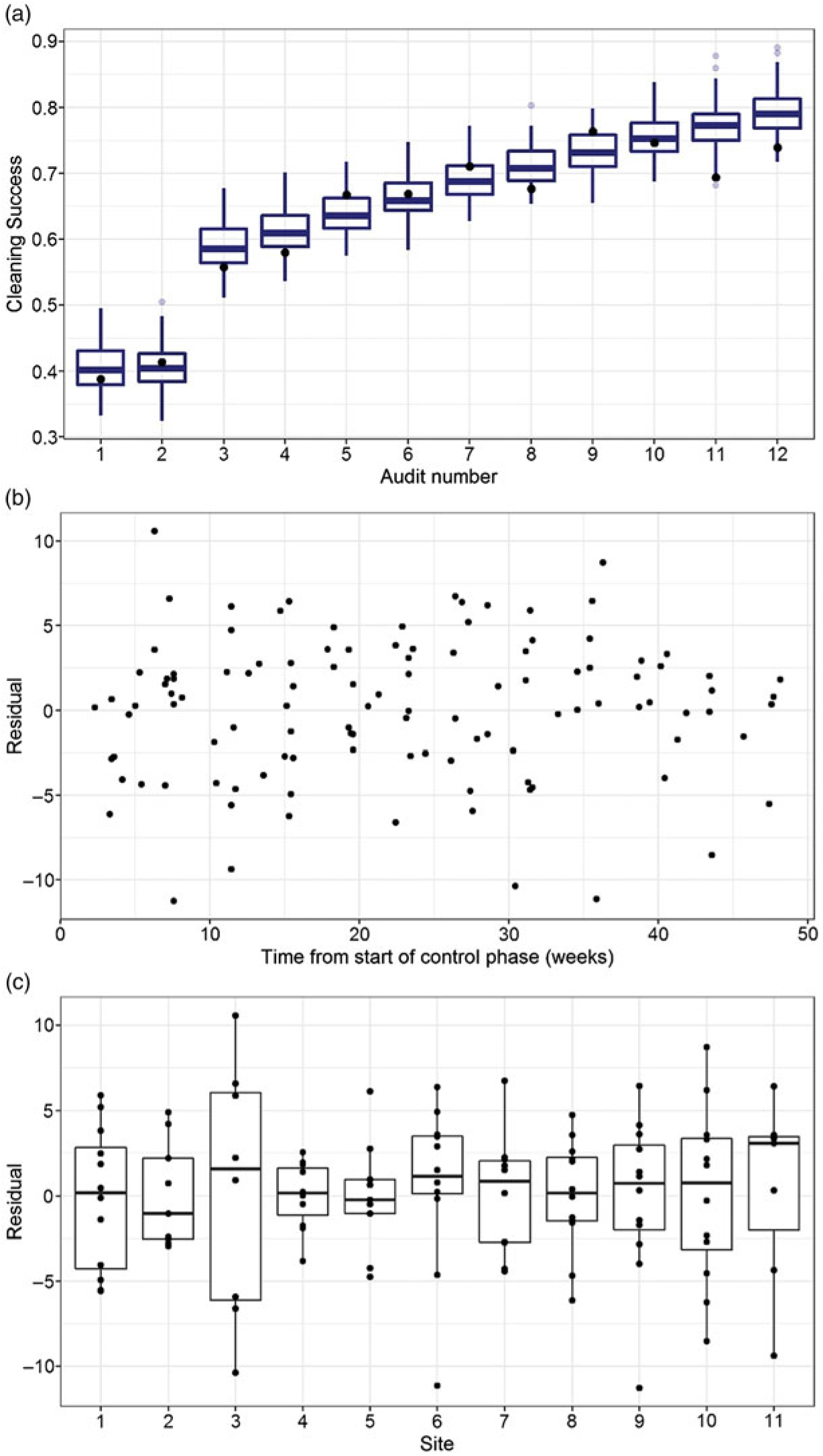
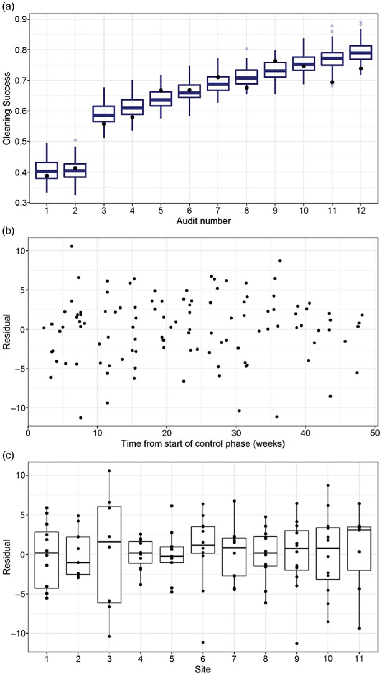
The model assessment for our selected model (model 3) is summarized in Figure 4. Simulation results showed a high level of overall agreement between observed versus predicted cleaning performance (Fig. 4a). Residual plots over time (Fig. 4b) did not indicate unexplained temporal correlation; however, residual plots by site (Fig. 4c) identified large negative residuals for 2 sites (sites 6 and 9). Follow-up analysis revealed unexpected poor performance recorded for 1 audit in the control phase (site 6) and 1 audit in the late intervention phase (site 9). Refitting the model without these observations did not impact parameter estimates, and therefore, these data were retained in the dataset.
Assessment of model 3 (binary change + linear intervention trend): (a) comparison of observed cleaning performance and model-based simulations by audit (black = observed sample means; grey = outlying simulations); (b) residuals versus time since the start of the control period; (c) boxplots of residuals by site.
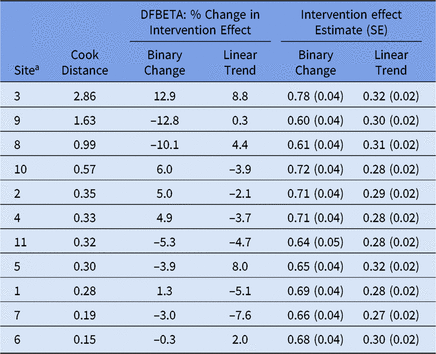
Using the Cook distance, we identified 2 sites (sites 3 and 9) as potentially influencing model results (Table 3). These 2 sites had the largest impact on the estimated binary effect, reflected in the percentage changes using DFBETA. However, the absolute effect of excluding each of these sites was small, with parameter estimates varying between 0.61 and 0.78 for the binary change and between 0.27 and 0.32 for the linear trend.
Influence Diagnostics for Assessing the Contribution of Each Hospital to the Estimated Intervention Effects

Note. SE, standard error.
a Sites are ordered by decreasing Cook distance. Estimated intervention effects following the exclusion of each site are also provided, to show the impact on model results.
Presenting the Results
Hypothesis testing summarizes the statistical significance of the intervention effect and other fixed effects included in a GLMM. P values should always be presented with parameter estimates and corresponding standard errors or confidence intervals because a statistically significant result does not provide information on the size of an effect.Reference Greenland, Senn and Rothman32
Predictions from the final model are recommended to help readers visualize the impact of the intervention over time. Point estimates of predictions are easily obtained in statistical packages, for example, using the ‘predict’ function in R. Alternatively, bootstrapping can be used to generate model-based predictions and corresponding uncertainty. Bootstrapping is a resampling approach for generating summary statistics when the true distribution is not available analytically.Reference Davison and Hinkley33 In R, bootstrapping is available in the lme4 package via the ‘bootMer’ function.Reference Bates, Mächler, Bolker and Walker15
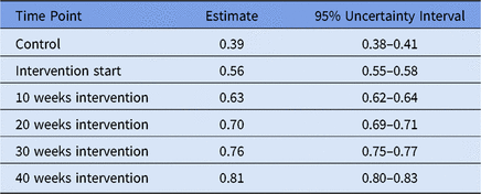
Results from our study indicated a statistically significant increase in the odds of cleanliness after introducing the bundle (odds ratio [OR], 1.94; 95% CI, 1.81–2.13; P < .001), which continued to improve over the intervention phase (OR, 1.34; 95% CI, 1.30–1.38; P < .001). Model-based predictions using bootstrapping (Table 4) showed that introducing the cleaning bundle immediately improved expected cleaning performance from 39% (95% uncertainty interval, 38%–41%) in the control period to 56% (95% uncertainty interval, 55%–58%) at the start of the intervention. At 40 weeks post-intervention, predicted cleaning performance improved further to 81% (95% uncertainty interval, 80%–83%).
Predicted Cleaning Thoroughness Under Model 3 During Control and Intervention Periods, Based on Results of Bootstrapping

Discussion
Multisite intervention studies are a common study design in infection control research. In this article, we have shown how GLMMs are ideally suited to analyzing multisite data over time. Using data collected from a case study in environmental cleaning, we have provided guidance on the main stages of GLMM analysis. When assessing a model, we recommend that residual plots be used to check for problems with the model or data. Researchers should also check for influential sites. Finally, when communicating model findings, the results of hypothesis testing should be accompanied by model predictions to summarize the effect of an intervention or policy change on outcomes over time. Overall, GLMMs are a flexible set of models that are worth learning.
Supplementary Material
To view supplementary material for this article, please visit https://doi.org/10.1017/ice.2019.114
Author ORCIDs
Nicole White 0000-0002-9292-0773; Adrian Barnett 0000-0001-6339-0374
Acknowledgments
We thank the Editor and reviewer for providing feedback on the original manuscript, and additional feedback from collaborators Brett Mitchell and Robin Blythe. The authors also thank the 11 hospitals that participated in the REACH study. The contents of the published material are solely the responsibility of the administering institution, participating institutions, and the individual authors; they do not reflect the views of the NHMRC.
Financial support
The REACH study is a National Health and Medical Research Council (NHMRC)-funded 2014–2017 Partnership Project (grant no. GNT1076006), led by Queensland University of Technology in conjunction with Wesley Medical Research. Industry partners Kimberly-Clark, Ecolab, and Whiteley provided financial and equipment (software and consumables) resources to support data collection but had no role in the study design, implementation or analysis. Adrian Barnett is funded by an NHMRC fellowship (grant no. APP1117784).
Conflicts of interest
All authors report no conflicts of interest relevant to this article.