


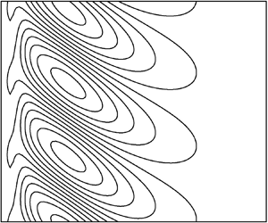

1. Introduction
Instabilities in fluids driven by the presence of both temperature and salinity gradients have been of significant interest since Stern (Reference Stern1960) realized that the mechanism driving the ‘oceanographic curiosity’ of Stommel, Arons & Blanchard (Reference Stommel, Arons and Blanchard1956) did not need a pipe. Stommel et al. (Reference Stommel, Arons and Blanchard1956) had the idea that a vertical pipe in a area of the sea where the surface water was hotter and saltier than at the bottom could sustain a continuous vertical flow. Less salty water in the pipe drawn from lower down would be heated through the pipe by the warmer surroundings. The water in the pipe would become relatively buoyant, and so would rise further. Stern (Reference Stern1960) realized that the pipe was not necessary as the much smaller diffusivity of salt in water compared to that of heat meant that a vertical column of water moving upwards essentially retained its lack of salt compared to its surroundings while absorbing heat. A similar mechanism would allow downward moving columns of fluid to retain their salt and continue their descent, giving rise to ‘salt fingers’ that have been observed in the laboratory and in the oceans. The realization that novel instabilities could be driven by the difference in the diffusivities of heat and salt gave rise to the whole field of double-diffusive convection where many such motions were investigated (Turner Reference Turner1974; Schmitt Reference Schmitt1994; Radko Reference Radko2013).
One of the areas of interest were double-diffusive instabilities driven by horizontal gradients of temperature and salinity. These had applications in a variety of areas such as fronts between bodies of water in the oceans, icebergs melting in the seas, salt-gradient solar ponds and magma chambers where layer-like instabilities may form. There was much study of these instabilities in laboratory experiments as well as in the field. However, theoretical studies of the onset of instabilities were often based around idealized cases where the background state was steady, such as motions in a vertical or inclined slot (Hart Reference Hart1971; Thangam, Zebib & Chen Reference Thangam, Zebib and Chen1981; Young & Rosner Reference Young and Rosner1998; Kerr & Tang Reference Kerr and Tang1999), or cases where a quasi-static assumption could be made and the background state was assumed to be steady (Kerr Reference Kerr1989, Reference Kerr1991). In this paper we will look at cases where neither of these idealizations are appropriate.
When a uniform salinity gradient is heated from a vertical sidewall, the heat that diffuses into the fluid from the boundary generates an upward motion. This in turn creates horizontal salinity gradients. Thus there are three components, the horizontal gradients of heat and salt and the vertical shear, that can drive or inhibit instabilities along with the vertical salinity gradient. This is shown schematically in figure 1. In some circumstances the initial instabilities that are observed can take the form of almost horizontal convecting layers (for example, Chen, Briggs & Wirtz Reference Chen, Briggs and Wirtz1971). While for other cases the convection cells are often observed to have an order-one aspect ratio (see, for example, Narusawa & Suzukawa Reference Narusawa and Suzukawa1981; Tanny & Tsinober Reference Tanny and Tsinober1988; Schladow, Thomas & Koseff Reference Schladow, Thomas and Koseff1992). Most of the experiments of Schladow et al. (Reference Schladow, Thomas and Koseff1992) had the added complexity of a vertical temperature gradient away from the wall in addition to the salinity gradient. In some examples instabilities seemed to emerge from a rising boundary layer (Wirtz, Briggs & Chen Reference Wirtz, Briggs and Chen1972). It is the initial linear growth of the instability that concerns us here. The complex nonlinear development of the convection layers when they reach a large enough amplitude is beyond the scope of this paper, although a focus of many of the experiments.
Schematic diagram of the heating of a salinity gradient from a vertical sidewall.

In some circumstances, such as the gradual heating of a strong salinity gradient, the instabilities start to grow when the heated thermal layer near the wall is quite wide in comparison to the vertical scale of the disturbances that initially form. In such cases a quasi-static analysis of the instabilities can be applicable, as conducted by Kerr (Reference Kerr1989). Then the results were in good agreement with some of the results of experiments such as Chen et al. (Reference Chen, Briggs and Wirtz1971) and Tanny & Tsinober (Reference Tanny and Tsinober1988) in the parameter regimes where the analysis was appropriate. However, in the case where the wall heating was such that instabilities formed more quickly, the quasi-static assumption was not valid. The agreement was not as good, as is to be expected. This is the case where the salinity gradients are weaker, or the heating increase occurs more rapidly. In these cases the evolution of the background state is on a comparable time scale to that of the growth of the instabilities, and so a conventional stability analysis is not applicable.
In the experiments of Tanny & Tsinober (Reference Tanny and Tsinober1988) the salinity gradients had a variety of wall heating rates applied. Some being very close to an instantaneous increase in wall temperature, while others had a more gradual increase over an extended period. In each case the wall temperature was continually monitored, and the instantaneous thermal and salt Rayleigh numbers based on the penetration depth of the background temperature from the wall were calculated:
 \begin{equation} {\mbox{Ra}}_T(t)=\frac{g\alpha{\rm \Delta} T(t) \delta^{3}}{\nu\kappa_T},\quad {\mbox{Ra}}_S(t)=\frac{g(-\beta\bar{S}_z)\delta^{4}}{\nu\kappa_T},\quad\mbox{where } \delta=(\kappa_Tt)^{1/2}.\end{equation}
Here,  $g$ is the acceleration due to gravity,
 $\alpha$ the coefficient of thermal expansion,
 $\beta$ the equivalent for salt,
 ${\rm \Delta} T(t)$ the instantaneous wall temperature,
 $\bar {S}_z$ the uniform vertical salinity gradient,
 $\nu$ the kinematic viscosity,
 $\kappa _T$ the thermal diffusivity and
 $t$ the time since the onset of wall heating. For each experiment the values of these Rayleigh numbers were tracked in the
 ${\mbox {Ra}}_S$–
 ${\mbox {Ra}}_T$ plane. The locations of these instantaneous Rayleigh numbers move up and to the right. These trajectories have gradients between 3/4 and 5/4 in the log–log plot they used, depending on the form of the heating. At the instant Tanny & Tsinober (Reference Tanny and Tsinober1988) first observed instabilities in the middle of the heated wall they recorded the position on the plot. These locations are reproduced in figure 2. In addition the trajectories of the points
 $( {\mbox {Ra}}_S(t), {\mbox {Ra}}_T(t))$ for four idealized experiments with slope 3/4 are shown by the arrows in this figure. These would correspond to cases with an instantaneous increase in the wall temperature. These four will be looked at in some detail in § 4. Tanny & Tsinober (Reference Tanny and Tsinober1988) made a comparison between the location of the experimental points to the stability boundary for the lateral heating of a salinity gradient in a vertical slot found by Thangam et al. (Reference Thangam, Zebib and Chen1981). The comparison of the instantaneous temperature and salt Rayleigh numbers to the stability boundary of the lateral heating of a salinity gradient in a vertical slot was a logical thing to do, given the absence of any other theoretical results at the time. However, the original marginal stability results for a vertical slot that they used had some errors that were corrected by Young & Rosner (Reference Young and Rosner1998) and Kerr & Tang (Reference Kerr and Tang1999). This corrected stability boundary is included in figure 2. Kerr & Tang (Reference Kerr and Tang1999) showed that the stability boundary for a slot in the
 ${\mbox {Ra}}_T$–
 ${\mbox {Ra}}_S$ plane for a Prandtl number and salt/heat diffusivity ratio appropriate for common salt in water has sections corresponding to 5 different asymptotic regimes. For example, one of these was the strong salinity gradient limit which was found by Hart (Reference Hart1971) for a vertical slot, and at leading order involves many of the approximations as the quasi-static analysis of Kerr (Reference Kerr1989) for an isolated heated vertical wall. However, some of the slot modes were unlikely to correspond directly to instabilities in a semi-infinite fluid. One of the regimes corresponded to a long wavelength instability up the slot, and so was incompatible with instabilities observed in experiments that seemed to be constrained by the Chen scale given by (2.9). This scale corresponds to the height a parcel of fluid in the salt stratification would rise by in order to be at the level of fluid with its new density if its temperature were to increase by
 ${\rm \Delta} T$. The heating of a uniform body of fluid without a salinity gradient at an isolated wall occurs for thermal Rayleigh numbers much smaller than those of the small
 ${\mbox {Ra}}_S$ limit in a slot, which one would expect to tend to the purely thermal case (Foster Reference Foster1965, Reference Foster1968; Kerr & Gumm Reference Kerr and Gumm2017). There are no clear reasons why the other asymptotic regimes for instabilities at a vertical slot would correspond particularly closely to those found when heating an isolated vertical wall.
Comparison of the instantaneous Rayleigh numbers,  ${\mbox {Ra}}_T$ and
 ${\mbox {Ra}}_S$, at the onset of instability for experimental results of Tanny & Tsinober (Reference Tanny and Tsinober1988) with the marginal stability curve for a laterally heated vertical slot (Young & Rosner Reference Young and Rosner1998; Kerr & Tang Reference Kerr and Tang1999). Also shown (dotted line) is the stability boundary of Kerr (Reference Kerr1989). The arrows, A–D, show trajectories of instantaneous Rayleigh numbers in typical experiments.

It is clear from many of the experimental results that the evolution of the instability is on a similar time scale to the evolution of the background state. For example, Schladow et al. (Reference Schladow, Thomas and Koseff1992) made the observations that the growth of instabilities seemed to start at the same time as the initial rise of the fluid up the wall came to a halt. In such cases the quasi-static assumption is not valid, and the analysis of Kerr (Reference Kerr1989) is not applicable to many observations. The objective of this paper is to rectify this situation.
A more recent approach to looking at instabilities in evolving systems was developed by Kerr & Gumm (Reference Kerr and Gumm2017). They investigated linear instabilities at isolated horizontal and vertical heated boundaries, and followed the evolution of the disturbances as the background state evolved. In their approach they looked for the initial state that maximized the growth of an energy-like quadratic measure of the amplitude of the instabilities over a fixed time interval. This was achieved by converting this maximization problem for their numerical simulations into a matrix eigenvalue problem. An important element of their method was the choice of the quadratic measure that was to be used. This measure involved all the components of the instability, but the relative ratio of the contributions from the velocity and temperature perturbations could be varied. The choice of this ratio was an important part of the optimization process. Inappropriate choices of the ratio of the velocity and temperature contributions in this measure could lead to an artificial apparent boost in the growth in the instabilities, while using a measure that focused on, say, just the kinetic energy could lead to an initial drop in the measure that underestimated the underlying growth. A choice of a quadratic measure that minimized the maximum growth over all possible initial conditions over the given time interval was found to be most effective. This approach was extended to double-diffusive instabilities that occur when a salinity gradient is heated from a lower boundary by Kerr (Reference Kerr2019). We use this method here.
There are three obvious different idealized cases of wall heating that could be considered. The first is the case of a sudden increase in the wall temperature by a fixed amount. Many experiments aim for such a fixed increase in wall temperatures. Although, in reality, there will be a time lag in attaining this final temperature. The second idealization is a constant heat flux, which results in the wall temperature growing like  $t^{1/2}$, such as the experiments of Narusawa & Suzukawa (Reference Narusawa and Suzukawa1981). Most experiments seem to have an early phase where the temperature grows linearly with time. Indeed, Tanny & Tsinober (Reference Tanny and Tsinober1988) sought to have linear temperature growth in some of their experiments. This was achieved by the computer control of the wall heating. Having a constant linear temperature increase after some initial time is the third obvious case, and is a good approximation for the early stages of nearly all experiments. In the logarithmic plot, as shown in figure 2, the trajectories of the instantaneous Rayleigh numbers in these three cases will be straight lines with gradients 3/4, 1 and 5/4 respectively. We will look at two of these cases – the first and the third, which correspond to the fixed temperature rise and the temperature increasing linearly with time. We shall see these two cases share many similarities. The second case lies, in some sense, between these two extremes.
In this paper we will look briefly in § 2 at the background state and some of the length scales that are associated with this problem. There are several of these length scales which may be more or less important in different regimes. This will be followed, in § 3, by a look at the governing equations for the instabilities, and a brief description of the approach used to investigate the instabilities. In § 4 we will consider instabilities when there is a sudden increase in wall temperature by a fixed amount,  ${\rm \Delta} T$. Here the natural focus will be on instabilities that occur when the salinity gradient is weaker. The sudden increase in wall temperature was looked at by Kerr & Gumm (Reference Kerr and Gumm2017) for heating a fluid at a sidewall in the absence of a salinity gradient. In this sudden-heating regime the trajectories of the instantaneous Rayleigh number follow lines with slope 3/4 in the
 $\log$–
 $\log$ Rayleigh number plane. They approach the marginal stability line of the quasi-static analysis of Kerr (Reference Kerr1989), that is valid when the salinity gradient is stronger, from the unstable side. The marginal stability line in that case corresponds to a line of slope 5/6 in this
 $\log$–
 $\log$ plane. This quasi-static regime is, however, accessible when the wall temperature increase is proportional to the time since the onset of heating, and the trajectories follow lines with slope 5/4. This regime is examined in § 5, where we will focus more on the cases with a stronger salinity gradient. This will be followed by further discussions and conclusions in the final section.
As we shall see later, there are four non-dimensional numbers that determine the behaviour of a salt-stratified fluid heated from a sidewall. Two of these are the Rayleigh numbers mentioned above that are a measure of the strength of the heating and the salinity gradients. The other two that we use are the Prandtl number,  $\sigma =\nu /\kappa _T$, and the ratio of the diffusivity of salt to the heat diffusivity,
 $\tau =\kappa _S/\kappa _T$. In order to make this problem tractable we will restrict ourselves to the case of
 $\sigma =7$ and
 $\tau =1/80$, the approximate values for water with common salt as used in laboratory experiments.
2. Background state and scales
In this section we will consider the background state that is observed when heating a semi-infinite uniform salinity gradient from a vertical sidewall, and some of the length scales that are associated with this flow.
The governing equations for the background state when heating a sidewall allow for a solution that is uniform in the vertical direction, and which only depends on the time since the onset of heating,  $t$, and the horizontal distance from the wall,
 $x$. The equations for this background state are
 \begin{gather} \frac{\partial \bar{W}}{\partial t}=g(\alpha\bar{T}-\beta\bar{S})+\nu\frac{\partial^{2}\bar{W}}{\partial x^{2}}, \end{gather}
 \begin{gather}\frac{\partial \bar{T}}{\partial t}=\kappa_T\frac{\partial^{2}\bar{T}}{\partial x^{2}}, \end{gather}
 \begin{gather}\frac{\partial \bar{S}}{\partial t}+\bar{W}\bar{S}_z=\kappa_S\frac{\partial^{2}\bar{S}}{\partial x^{2}}, \end{gather}
where the vertical velocity is  $\bar {W}(x,t)$, the temperature is
 $T=T_0+\bar {T}(x,t)$ and the salinity is
 $S=S_0+z\bar {S}_z+\bar {S}(x,t)$ with the vertical salinity gradient
 $\bar {S}_z$ constant. We have made the Boussinesq approximation and assumed the density of the fluid depends linearly on the temperature and salinity
 \begin{equation} \rho=\rho_0(1-\alpha(T-T_0)+\beta(S-S_0)). \end{equation}
The initial conditions are that the fluid is at rest, and the temperature and salinity variations are zero at the time of the onset of heating. The boundary conditions are no slip for the vertical velocity, a prescribed temperature at the wall and zero flux of salt through the wall. Far from the wall the motions and the temperature and salinity remain unchanged. That is to say
 \begin{gather} \bar{W}(x,0)=\bar{T}(x,0)=\bar{S}(x,0)=0\quad\mbox{for } x>0, \end{gather}
 \begin{gather}\bar{W}(0,t)=0,\quad\bar{T}(0,t)={\rm \Delta} T(t),\quad \frac{\partial \bar{S}}{\partial x}(0,t)=0\quad\mbox{for } t>0, \end{gather}
 \begin{gather}\bar{W}(x,t)\to 0,\quad\bar{T}(x,t)\to 0,\quad\bar{S}(x,t)\to 0\quad \mbox{as } x\to\infty. \end{gather}
A condition that is often applied to problems of lateral heating in a slot is that there is no total flux of fluid up the slot. This is not appropriate for a semi-infinite fluid. Even though we will be making our numerical calculations in a slot, the far wall will play an insignificant role. We do not impose a zero vertical flux condition on our calculations.
If we impose a sudden temperature increase of a fixed  ${\rm \Delta} T$ at time
 $t=0$. The temperature equation has the well-known solution
 \begin{equation} \bar{T}(x,t)={\rm \Delta} T\, {\rm erfc}\left(\frac{x}{2(\kappa_Tt)^{1/2}}\right), \end{equation}
where  ${\rm erfc}(x)$ is the complementary error function. However, the vertical velocity and salinity do not have simple closed-form solutions such as this. The small- and large-time asymptotics of these equations can be found (see Kerr Reference Kerr1989). For small times the horizontal length scale is just
 \begin{equation} L_1=(\kappa_T t)^{1/2}, \end{equation}
the thermal diffusion distance. For large times it can be shown that there are two additional distinct length scales that emerge. One is associated with a salt boundary layer and the other associated with oscillations generated in the fluid at the Brunt–Väisälä or buoyancy frequency,  $N$, given by
 $N^{2}=-g\bar {\rho }_z/\rho _0$ (Rayleigh Reference Rayleigh1883). These length scales are
 \begin{equation} L_2=\left(\frac{4\kappa_S\nu}{g\beta(-\bar{S}_z)}\right)^{1/4},\quad L_3=((\nu+\kappa_S)t/2)^{1/2}, \end{equation}
respectively. The contributions of these two components both decay at  $t^{-1/2}$ for the case of a no-flux boundary condition on the salt at the wall. This enabled Kerr (Reference Kerr1989) to focus on the disturbances on the thermal scale,
 $L_1$, for his quasi-static large-time analysis of the resulting instabilities. However, for the problems of interest here, near the onset of heating the three components identified with the large-time asymptotics may not have separated out.
The above scales are also present for the case of linear wall heating where the temperature profile is given by
 \begin{equation} \bar{T}(x,t)=C\left(\left(t+\frac{x^{2}}{2\kappa_T}\right) {\rm erfc} \left(\frac{x}{2(\kappa_Tt)^{1/2}}\right)-\frac{x}{( {\rm \pi}\kappa_T t)^{1/2}}\exp\left(-\frac{x^{2}}{4\kappa_Tt}\right)\right), \end{equation}
with the wall temperature  $\bar {T}(0,t)=Ct$ for some constant
 $C$.
If a weak salinity gradient has a large temperature difference imposed, then one may expect that the salinity gradient is relatively unimportant, and so the scalings from Kerr & Gumm (Reference Kerr and Gumm2017) when they looked at the heating of a body of fluid from the side would be appropriate. There the length scale,  $L_4$, that made the thermal Rayleigh number one was adopted
 \begin{equation} {\mbox{Ra}}_T=\frac{g\alpha{\rm \Delta} T L_4^{3}}{\nu\kappa_T}=1. \end{equation}
This scale was used by Foster (Reference Foster1965) in his investigation of heating a body of fluid from below, and may be appropriate when the salinity gradient is weak. As we have two Rayleigh numbers there would be a second length scale that could be derived by setting  ${\mbox {Ra}}_S=1$. It is not clear in advance which, if either, would be appropriate here in general.
In addition to these horizontal length scales there is a vertical scale, the so-called Chen scale (Chen et al. Reference Chen, Briggs and Wirtz1971), given by
 \begin{equation} H_C=\frac{\alpha{\rm \Delta} T}{-\beta\bar{S}_z},\end{equation}
which describes the height a parcel of fluid in the isothermal density gradient would rise if it were to be heated by  ${\rm \Delta} T$ in order to be surrounded by fluid of equal density. With a fixed wall temperature, this length scale is also fixed. For increasing wall temperatures this scale will also increase with time. The average vertical scale of well-developed instabilities in experiments of heating or cooling a salinity gradient is often found to be of the order of 60 %–70 % of this Chen scale (Wirtz et al. Reference Wirtz, Briggs and Chen1972; Huppert & Josberger Reference Huppert and Josberger1980; Huppert & Turner Reference Huppert and Turner1980; Tanny & Tsinober Reference Tanny and Tsinober1988).
Having the Chen scale smaller than the width of the thermal layer allows a stability analysis to be carried out using a quasi-static assumption, where the thermal length scale,  $L_1$, was appropriate for the horizontal scale and the Chen scale,
 $H_C$, for the vertical scales. This was conducted by Kerr (Reference Kerr1989). The theoretical results were in good agreement with the results of experiments such as Chen et al. (Reference Chen, Briggs and Wirtz1971) and Tanny & Tsinober (Reference Tanny and Tsinober1988) in the cases where the analysis was appropriate. However, when the quasi-static assumption was not valid the agreement was not as good. Unfortunately there is no one length scale that is the most appropriate in all circumstances. In the analysis of Kerr (Reference Kerr1989) the predicted instabilities were thin, almost horizontal layers as were observed in the experiments of, say, Chen et al. (Reference Chen, Briggs and Wirtz1971). It was found in Kerr (Reference Kerr1989) that the appropriate non-dimensional parameter for predicting the onset of instability in this quasi-static limit was
 \begin{equation} Q=\frac{(1-\tau)^{6}g(\alpha {\rm \Delta} T)^{6}}{\nu\kappa_SL_1^{2} \left(-\beta\bar{S}_z\right)^{5}}=\frac{(1-\tau)^{6}g\alpha {\rm \Delta} T H_C^{5}}{\nu\kappa_SL_1^{2}},\end{equation}
where  $\tau =\kappa _S/\kappa _T$ is the salt/heat diffusivity ratio. The parameter
 $Q$ involves both the horizontal thermal scale,
 $L_1$, and the vertical Chen scale,
 $H_C$. The factor
 $(1-\tau )^{6}$ leads to simplification of the equations in the mathematical analysis and is not of importance here. From this we can see that not only is there no single length scale that is appropriate everywhere, but in some circumstances more than one scale is needed.
We will now look at the background state. Having found several length scales for the full problem, we will now use a variation of  $L_2$ to non-dimensionalize the equations for the background flow for the fixed wall temperature rise of
 ${\rm \Delta} T$. We non-dimensionalize (2.1) using the scalings
 \begin{gather} x=\left(\frac{\nu\kappa_T}{g\beta(-\bar{S}_z)}\right)^{1/4}\hat{x}, \quad t=\left(\frac{\nu}{\kappa_Tg\beta(-\bar{S}_z)}\right)^{1/2}\hat{t}, \end{gather}
 \begin{gather}\bar{W}=\left(\frac{g(\alpha{\rm \Delta} T)^{2}\kappa_T}{\nu\beta(-\bar{S}_z)}\right)^{1/2} \hat{W},\quad \bar{T}={\rm \Delta} T\hat{T},\quad \bar{S} = \frac{\alpha{\rm \Delta} T}{\beta} \hat{S}. \end{gather}
The resulting equations for the background flow are
 \begin{gather} \frac{1}{\sigma}\frac{\partial \hat{W}}{\partial \hat{t}}=\hat{T}-\hat{S}+\frac{\partial^{2}\hat{W}}{\partial \hat{x}^{2}}, \end{gather}
 \begin{gather}\frac{\partial \hat{T}}{\partial \hat{t}}=\frac{\partial^{2}\hat{T}}{\partial \hat{x}^{2}}, \end{gather}
 \begin{gather}\frac{\partial \hat{S}}{\partial \hat{t}}-\hat{W}=\tau\frac{\partial^{2}\hat{S}}{\partial \hat{x}^{2}}. \end{gather}
The boundary conditions at the wall are  $\hat {T}=1$, along with the no-flux condition on the salinity and no slip for the velocity along with the decay conditions as
 $\hat {x}\to \infty$. We see that this problem for the background state only depends on the Prandtl number and salt/heat diffusivity ratio. Thus, in these units the background evolution is the same for all cases, and so if we want to find the time taken to achieve the maximum kinetic energy of the background flow, or the time to the first minimum, then there is a universal answer.
A plot of the kinetic energy of the background flow in these units,
 \begin{equation} E_{BG}(\hat{t})=\int_0^{\infty}\tfrac{1}{2}\hat{W}(\hat{x},\hat{t})^{2}\,\textrm{d}\hat{x}, \end{equation}
is shown in figure 3(a). This shows an increase as the heated fluid rises to the wall temperature. Because of the salinity gradient the rising fluid becomes saltier than the fluid far from the wall, causing a decrease in the acceleration of the fluid up the wall and a peak in the kinetic energy. After this the energy decays away. This decaying tail has a modulation due to the stratification which is at the buoyancy frequency of  $\sigma ^{1/2}$ in these units. The first maximum occurs at
 $\hat {t}=1.140$ and first minimum at
 $\hat {t}=2.895$.
Graph of the kinetic energy of the background flow as a function of  $\hat {t}$ from (2.12) with temperature at the wall given by (a)
 $\hat {T}=1$ and (b)
 $\hat {T}=\hat {t}$.

Comparing (1.1a,b) and the scaling for  $t$ in (2.12) we see that the instantaneous salt Rayleigh number and
 $\hat {t}$ are linked by
 \begin{equation} {\mbox{Ra}}_S=\hat{t}^{2}. \end{equation}
Hence, the general form of the background flows is governed by the salt Rayleigh number only. The first maximum in the kinetic energy occurs when the instantaneous Rayleigh number is given by
 \begin{equation} {\mbox{Ra}}_S=(1.140)^{2}=1.300,\end{equation}
and the first minimum occurs when
 \begin{equation} {\mbox{Ra}}_S=(2.895)^{2}=8.381.\end{equation}
We shall refer to these quantities later.
The profiles of the background components will also only depend on  $\hat {t}$, and hence on
 ${\mbox {Ra}}_S$. A comparison of the salinity profiles to the temperature profiles is shown in figure 4 for
 ${\mbox {Ra}}_S=10^{-1}, 10^{0},\ldots , 10^{4}$. With these scalings given temperature and salinity perturbations have equal but opposite contributions to the density. These examples go from one extreme where the salinity is small in comparison to the temperature, so the flow is still dominated by the temperature. At the other extreme the profiles are almost identical, and so their effect on the density almost exactly cancel out and the buoyancy forcing is greatly reduced. The initial increase in the salinity is away from the wall near the location of the maximum of the vertical velocity. This results in some of the intermediate salinity profiles having significant regions near the wall with salinity gradients in the opposite direction to the bulk of the fluid.
Comparison of the background salinity profiles (solid lines) and temperature profiles (dashed lines) for the sudden increase in the wall temperature. Here, the salt Rayleigh numbers are (a)  ${\mbox {Ra}}_S=0.1$, (b)
 ${\mbox {Ra}}_S=1$, (c)
 ${\mbox {Ra}}_S=10$, (d)
 ${\mbox {Ra}}_S=10^{2}$, (e)
 ${\mbox {Ra}}_S=10^{3}$ and (f)
 ${\mbox {Ra}}_S=10^{4}$.

For the case where the wall temperature is given by  $T(0,t)=ct$ for
 $t>0$, if the scalings for
 $x$ and
 $t$ are those used before in (2.11), but now
 \begin{equation} \bar{W}=\frac{\alpha c}{\beta(-\bar{S}_z)}\hat{W},\quad \bar{T}=c\left(\frac{\nu}{\kappa_Tg\beta(-\bar{S}_z)}\right)^{1/2}\hat{T},\quad \bar{S}=\frac{\alpha c}{\beta}\left(\frac{\nu}{\kappa_Tg\beta(-\bar{S}_z)} \right)^{1/2}\hat{S},\end{equation}
the resulting equations are the same as (2.12), and the boundary conditions are unchanged, except for  $\hat {T}=\hat {t}$ at the wall. The growth of the kinetic energy is shown in figure 3(b). This time there is no maximum as the temperature continues to rise, with the energy growth being proportional to
 $t^{1/2}$ at leading order for large time. Again there is a modulation at the buoyancy frequency, but it is less pronounced. If we were to look at a salt-stratified fluid heated with a constant wall flux the kinetic energy would rise to a peak and then decay as
 $t^{-1/2}$, as would the maximum velocity. There is again a modulation at the buoyancy frequency on top of the general decay. Schladow et al. (Reference Schladow, Thomas and Koseff1992) observed in their experiments that the rise of the boundary layer flow come to a halt. This was for the case of a constant heat flux. However, there was also a vertical temperature gradient away from the wall, along with the vertical salinity gradient.
It should be noted that the scalings (2.11) and (2.17a–c) do not have a scaling for the velocity which is the scaling for the length divided by the scaling for time, as is more usual. If these scalings were to be used for the full equations, then new less conventional non-dimensional parameters would appear in the equations for the perturbations.
As we will be aiming to understand the instabilities that are observed experimentally, we will adopt the approach of Tanny & Tsinober (Reference Tanny and Tsinober1988) and fix on the final time when observations are made or when the experiment is terminated. It was argued by Kerr (Reference Kerr2000) that this latter time was important in some experiments in determining whether instabilities were seen or not. We will focus the instantaneous Rayleigh numbers, (1.1a,b), at this final moment, giving us a time scale,  $t_1$, and the associated thermal length scale,
 $L_1=(\kappa _Tt_1)^{1/2}$. If we non-dimensionalize
 $t$ with respect to this time, then the end time will automatically be
 $t_1=1$. However, we will refer
 $t_1$ as a shorthand for the end time henceforth.
3. Governing equations for instabilities and solution method
In this section we will give the governing equations for the linear instabilities to the evolving background state and give an outline of the approach for finding the optimal instabilities. Fuller details of this approach can be found in Kerr & Gumm (Reference Kerr and Gumm2017) and Kerr (Reference Kerr2019).
The linearized equations for the perturbations to the velocity,  $\boldsymbol {u}$, and the temperature,
 $T$, are
 \begin{gather} \frac{\partial \boldsymbol{u}}{\partial t}+\bar{W}(x,t) \frac{\partial\boldsymbol{u}}{\partial z}+\boldsymbol{u}\boldsymbol{\cdot} \boldsymbol{\nabla}\bar{W}(x,t)\hat{\boldsymbol{z}}=-\frac{1}{\rho_0}\boldsymbol{\nabla} p+g\alpha T\hat{\boldsymbol{z}}-g\beta S\hat{\boldsymbol{z}}+\nu\nabla^{2}\boldsymbol{u}, \end{gather}
 \begin{gather}\boldsymbol{\nabla}\boldsymbol{\cdot}\boldsymbol{u}=0, \end{gather}
 \begin{gather}\frac{\partial T}{\partial t}+\bar{W}(x,t)\frac{\partial T}{\partial z}+u\frac{\partial}{\partial x}\bar{T}(x,t)=\kappa_T\nabla^{2}T, \end{gather}
 \begin{gather}\frac{\partial S}{\partial t}+\bar{W}(x,t)\frac{\partial S}{\partial z}+u\frac{\partial}{\partial x}\bar{S}(x,t)+w\bar{S}_z=\kappa_S\nabla^{2}S, \end{gather}
where  $\bar {W}(x,t), \bar {T}(x,t)$ and
 $\bar {S}(x,t)$ are the background vertical velocity and temperature variations from the previous section, and
 $\bar {S}_z$ the uniform vertical salinity gradient. The unit vector pointing upwards is
 $\hat {\boldsymbol {z}}$. Here, we have made the Boussinesq approximation and assumed a linear equation of state.
In this study we will restrict ourselves to looking at two-dimensional motions, and so we can use the vorticity–streamfunction formulation. We take the curl of the momentum equation (3.1a) and consider the  $y$-component of the vorticity,
 $\omega$. We will non-dimensionalize the equations using the rescalings
 \begin{equation} \boldsymbol{x'}= \boldsymbol{x}/D,\quad t'=\kappa_T t/ D^{2},\quad \omega'= D^{2}\omega/\kappa_T,\quad T'=T/{\rm \Delta} T,\quad S'=S/(-D\bar{S}_z), \end{equation}
where  $D$ is an appropriate length scale. For example, in the case of two parallel boundaries the distance between the walls is an obvious and conventional choice of a length scale for non-dimensionalizing the equations. However, for heating a salinity gradient from a sidewall we will use
 $D=L_1=(\kappa _Tt_1)^{1/2}$, where
 $t_1$ is the fixed time at the end of the real or numerical experiment.
The non-dimensional background equations are
 \begin{gather} \frac{1}{\sigma}\frac{\partial \bar{W}'}{\partial t'}= {\mbox{Ra}}_T\bar{T}'- {\mbox{Ra}}_S\bar{S}'+\frac{\partial^{2}\bar{W}'}{\partial x'^{2}}, \end{gather}
 \begin{gather}\frac{\partial \bar{T}'}{\partial t'}=\frac{\partial^{2}\bar{T}'}{\partial x'^{2}}, \end{gather}
 \begin{gather}\frac{\partial \bar{S}'}{\partial t'}-\bar{W}'=\tau\frac{\partial^{2}\bar{S}'}{\partial x'^{2}}. \end{gather}
The equations for the vorticity and the streamfunction,  $\psi '$ are
 \begin{gather} \frac{1}{ \sigma}\left(\frac{\partial \omega'}{\partial t'}-\frac{\partial \psi'}{\partial z'}\frac{\partial^{2}\bar{W}'}{\partial x'^{2}}+\overline{W'}\frac{\partial \omega'}{\partial z'}\right)=- {\mbox{Ra}}_T\frac{\partial T'}{\partial x'}+ {\mbox{Ra}}_S\frac{\partial S'}{\partial x'}+\nabla'^{2}\omega', \end{gather}
 \begin{gather}\nabla'^{2}\psi'=-\omega', \end{gather}
where the primes indicate non-dimensional variables. The perturbation velocity components are given by
 \begin{equation} u'=-\frac{\partial \psi'}{\partial z'},\quad w'=\frac{\partial \psi'}{\partial x'}. \end{equation}
The perturbation temperature and salinity equations are then given by
 \begin{gather} \frac{\partial T'}{\partial t'}-\frac{\partial \psi'}{\partial z'}\frac{\partial \bar{T}'}{\partial x'}+\bar{W}'\frac{\partial T'}{\partial z'}=\nabla'^{2}T', \end{gather}
 \begin{gather}\frac{\partial S'}{\partial t'}-\frac{\partial \psi'}{\partial z'}\frac{\partial \bar{S}'}{\partial x'}-\frac{\partial \psi'}{\partial x'}+\bar{W}'\frac{\partial S'}{\partial z'}=\tau\nabla'^{2}S'. \end{gather}
Henceforth, we will drop the primes.
One boundary condition we apply at the wall is the no-slip condition for the velocity. As we have a prescribed temperature at the wall the perturbation will be zero. For the salinity we have zero flux at the wall. It should be noted that for the idealized case of a constant heat flux at the wall, the natural boundary condition at the wall would also be a no-flux condition. However, in real heat-salt experiments the walls are never perfectly conducting nor perfectly insulating, and so these idealized conditions will always be an approximation. We will stick to the perfectly conducting idealization of zero temperature perturbation for all our calculations. Far from the wall all perturbations tend to zero.
If we define the measure of a quantity  $F(x,z,t)$ to be
 \begin{equation} \langle F(x,z,t)\rangle =\int_0^{\infty}\frac{1}{P}\int_0^{P} F(x,z,t)\,\textrm{d}z\,\textrm{d} x, \end{equation}
where  $P$ is the vertical period of the instabilities, then we can define a quadratic energy-like measure of the amplitude of the linear disturbances by
 \begin{equation} E(t)=E_K(t)+\lambda E_T(t)+\mu E_M(t), \end{equation}
where
 \begin{equation} E_K(t)=\langle \tfrac{1}{2}|\boldsymbol{u}|^{2}\rangle,\quad E_T(t)=\langle \tfrac{1}{2}T^{2}\rangle,\quad E_M(t)=\langle \tfrac{1}{2}(S-\gamma T)^{2}\rangle. \end{equation}
The quantities  $\lambda , \mu$ and
 $\gamma$ are parameters that are to be determined in the stability analysis. The approach taken is to consider a time interval from
 $t=t_0$ to
 $t=t_1$ and find the initial disturbance that maximizes the growth of
 $E(t_1)/E(t_0)$, or equivalently maximizes
 $E(t_1)$ subject to the constraint
 $E(t_0)=1$. The outcome of this optimization of the growth depends of the parameters
 $\lambda , \mu$ and
 $\gamma$. In Kerr & Gumm (Reference Kerr and Gumm2017) thermal problems were considered with only
 $E_T(t)$ and the parameter
 $\lambda$. It was shown that by making
 $\lambda$ very big or very small the optimized growth could be made arbitrarily large. It was found that choosing
 $\lambda$ to minimize this optimal growth was a good choice. For example, when applied to the heating of a horizontal layer of fluid, the classic Rayleigh–Bénard problem, the maximum growth rate from conventional linear stability analysis was recovered, even when
 $t_1-t_0$ was relatively small. It was shown in Kerr (Reference Kerr2019) that, again, a good choice of the parameters
 $\lambda , \mu$ and
 $\gamma$ for double-diffusive problems was one that minimized this maximal growth found by optimizing the initial conditions. There it was also shown that the adoption of a mixed quadratic term,
 $E_M(t)$, instead of one just involving
 $S^{2}$, was more effective. A mixed term like this was also required in the energy stability analysis of Kerr (Reference Kerr1990). Even though this principle of minimizing the maximal growth has proved very effective, there is no fundamental reason yet identified that means it must be the best choice in all cases for investigating the stability of evolving systems such as those considered here and in Kerr & Gumm (Reference Kerr and Gumm2017) and Kerr (Reference Kerr2019). However, no alternative satisfactory contenders to this approach have been identified. We will then independently find the vertical period of the disturbances that maximizes the growth found with optimized
 $\lambda , \mu$ and
 $\gamma$.
We will adopt here the convenient constraint that  $E(t_0)=1$ in all cases. We will also consider two cases for the selection of
 $t_0$: instabilities that start growing at the onset of heating, that is to say
 $t_0=0$, and the case where
 $t_0>0$, which may lead to a larger growth in
 $E(t_1)$ by the end of the time interval. This leads to a further level of optimization.
The method we use for finding the most unstable modes was developed in Kerr & Gumm (Reference Kerr and Gumm2017) for thermal problems and Kerr (Reference Kerr2019) for double-diffusive problems, where more details are available. We look at modes with vertical wavenumber  $\alpha$. Then, for example, we express the temperature as
 \begin{equation} T(x,z,t)=\Re[T(x,t)\textrm{e}^{\textrm{i}\alpha z}]=T_r(x,t)\cos \alpha z-T_i(x,t)\sin\alpha z, \end{equation}
where  $T_r$ and
 $T_i$ are the real and imaginary parts of
 $T$. The evolution of the temperature, salinity, vorticity and streamfunction are then calculated over the time interval from
 $t=t_0$ to
 $t=t_1$ on a grid with
 $N$ interior points. So we evaluate numerical solutions that can be expressed as vectors such as
 \begin{equation} \boldsymbol{T}(t)=({T_r}_1,{T_r}_2,\ldots,{T_r}_{N},{T_i}_1,{T_i}_2,\ldots,{T_i}_{N})^\textrm{T}. \end{equation}
Previously, we had zero boundary conditions for the temperature, salinity and streamfunction, and so we only needed the interior values of these. The no-slip condition meant that we could determine the wall values of the velocity from the interior values. This time we have a no-flux condition for the salinity, and so we need to incorporate the wall values. The approximation for salinity will also include  ${S_r}_0, {S_i}_0, {S_r}_{N+1}, {S_r}_{N+1}$ We take vectors for the temperature, salinity and vorticity to give a combined vector
 \begin{equation} \boldsymbol{\varPsi}(t)=\left(\begin{array}{c}\boldsymbol{T}(t) \\ \boldsymbol{S}(t)\\ \boldsymbol{\omega}(t) \end{array}\right).\end{equation}
We can then express the numerical approximation to  $E(t)$ as
 \begin{equation} E(t)= \boldsymbol{\varPsi}(t)^\textrm{T}{\boldsymbol{\mathsf{A}}}(\lambda,\mu,\gamma) \boldsymbol{\varPsi}(t), \end{equation}
where  ${\boldsymbol{\mathsf{A}}}$ is a symmetric matrix. Our optimization becomes the finding of the initial vector
 $\boldsymbol {\varPsi }(t_0)$ with
 $E(t_0)=1$ which maximizes
 $E(t_1)$. As the problem is linear, we can calculate the transfer matrix,
 ${\boldsymbol{\mathsf{M}}}$, such that
 \begin{equation} \boldsymbol{\varPsi}(t_1)={\boldsymbol{\mathsf{M}}} \boldsymbol{\varPsi}(t_0), \end{equation}
for all possible initial conditions. This involves many numerical simulations over the time interval from  $t=t_0$ to
 $t=t_1$. Our optimization problem can now be expressed in matrix form as finding the vector
 $\boldsymbol {\varPsi }$ which maximizes
 \begin{equation} ({\boldsymbol{\mathsf{M}}} \boldsymbol{\varPsi})^\textrm{T}{\boldsymbol{\mathsf{A}}}({\boldsymbol{\mathsf{M}}} \boldsymbol{\varPsi}) \quad\mbox{with } \boldsymbol{\varPsi}^\textrm{T}{\boldsymbol{\mathsf{A}}} \boldsymbol{\varPsi}=1. \end{equation}
With the use of a Lagrange multiplier,  $\varLambda$, this maximization problem reduces to the eigenvalue problem
 \begin{equation} {\boldsymbol{\mathsf{M}}}^\textrm{T}{\boldsymbol{\mathsf{A}}} {\boldsymbol{\mathsf{M}}} \boldsymbol{\varPsi}={\boldsymbol{\mathsf{M}}}^\textrm{T} {\boldsymbol{\mathsf{A}}}{\boldsymbol{\mathsf{M}}}{\boldsymbol{\mathsf{A}}}^{-1} ({\boldsymbol{\mathsf{A}}} \boldsymbol{\varPsi})=\varLambda ({\boldsymbol{\mathsf{A}}} \boldsymbol{\varPsi}),\end{equation}
with eigenvector  ${\boldsymbol{\mathsf{A}}} \boldsymbol {\varPsi }$, and eigenvalue
 $\varLambda$. The largest such eigenvalue is the maximum growth in
 $E(t_1)$ that we seek. Fortunately, for the problems considered in this paper iterative methods for finding this eigenvalue and associated eigenvector proved to be quick and effective. The minimums of the growth rate as a function of
 $\lambda , \mu$ and
 $\gamma$ were smooth, and so the ratios of
 $E_K(t), E_T(t)$ and
 $E_M(t)$ at
 $t=t_0$ and
 $t=t_1$ are the same, as shown in Kerr (Reference Kerr2019). In the calculations we typically use
 $N=240$, but for some more extreme cases and for checking we use up to
 $N=480$.
4. Sudden increase in wall temperature
In this subsection we will look at the idealized case of the sudden increase in the wall temperature at  $t=0$. This was the aimed for case of Chen et al. (Reference Chen, Briggs and Wirtz1971), but the experiments took approximately 3 minutes to reach this final temperature. However, Tanny & Tsinober (Reference Tanny and Tsinober1988) were able to raise their wall temperature in a few seconds. Another set of experiments where there was a rapid change in the heat at a vertical wall were those of Huppert & Josberger (Reference Huppert and Josberger1980) and Huppert & Turner (Reference Huppert and Turner1980) where blocks of ice were introduced into a salinity gradient. Although the temperature was effectively a sudden decrease in temperature (fully equivalent to a sudden increase) there was the added difficulty in these cases of a flux of fresh water at the boundary due to the ice melting, and so comparisons with the work here could be problematic.
We look at the growth of linear instabilities for the idealized problem where the non-dimensional wall temperature is instantaneously raised by  $1$ at the initial time,
 $t=0$. In this case the instantaneous thermal and salt Rayleigh numbers (1.1a,b) are proportional to
 $t^{3/2}$ and
 $t^{2}$ respectively. Hence the points
 $( {\mbox {Ra}}_S, {\mbox {Ra}}_T)$ evolve along lines of slope 3/4 in the
 $\log$–
 $\log$ plot of the
 ${\mbox {Ra}}_S$–
 ${\mbox {Ra}}_S$ plane as shown in figure 2. We will base the presentation of many of our results on this approach, used by Tanny & Tsinober (Reference Tanny and Tsinober1988). Each point on the plot will correspond to the final Rayleigh numbers of a numerical experiment. At this point the growth of the instabilities will be investigated: we find the optimal growth and the corresponding wavenumber. We will consider two cases. Firstly those where the growth of instabilities is measured from the initial time
 $t_0=0$. Secondly, we will look at those where this initial time for measuring the growth of instabilities is also optimized to maximize the growth over the time interval from
 $t=t_0$ to
 $t=t_1$.
4.1. Growth of instabilities from  $t_0=0$

The optimal final growth,  $E(t_1)$, as a function of the final instantaneous
 ${\mbox {Ra}}_S$ and
 ${\mbox {Ra}}_T$ with
 $t_0=0$ is shown in figure 5. In each case the growth is minimized with respect to
 $\lambda , \mu$ and
 $\gamma$, and maximized with respect to the wavenumber,
 $\alpha$. This optimal wavenumber is shown in figure 6. (In these and subsequent contour plots shading has been added, with blue taking the lower values and red the higher. This is intended to aid clarity, particularly where there are discontinuities.) In figure 5 we only show the contours of the growth in
 $E(t)$ in the range from
 $10^{2}$ to
 $10^{16}$. The former corresponds to a growth in the perturbation quantities by a factor of approximately 10. The form of the instabilities changes over the growth period so this factor may not be exact for each component. The maximum figure of
 $10^{16}$ corresponds to a growth in velocities comparable to the ratio of the speed of fingernail growth to around 10 cm s
 $^{-1}$. In all probability, any linear disturbance will be of large amplitude, and be nonlinear in their nature, before this upper limit for growth is observed. Any growths much bigger are mathematically well defined but likely to be of limited physical significance, and so omitted so that the focus is on results that are likely to be relevant in reality.
Growth in  $E(t_1)$ as a function of final
 ${\mbox {Ra}}_S$ and
 ${\mbox {Ra}}_T$ with
 $t_0=0$. Contours with
 $E(t_1)=10^{2}, 10^{3}, \ldots , 10^{16}$ (from bottom to top). Also shown are arrows indicating the general evolution of the instantaneous Rayleigh numbers for four cases, A–D. The red dashed lines indicating the boundaries of the different regimes, and the black dotted line giving points corresponding to marginal stability for the large
 ${\mbox {Ra}}_S$ quasi-static asymptotics with
 $Q=147\,700$ (Kerr Reference Kerr1989).

Wavenumber,  $\alpha$, of most unstable mode as a function of final
 ${\mbox {Ra}}_S$ and
 ${\mbox {Ra}}_T$, with
 $t_0=0$. The contour lines are at
 $\alpha =10^{0}, 10^{\pm 0.1}, 10^{\pm 0.2}, 10^{\pm 0.5}, \ldots$, with the heavier lines at
 $\alpha =10^{0}, 10^{\pm 0.5}, 10^{\pm 1.0}, \ldots$ and the dashed contours have
 $\alpha <1$. The green dashed lines show the contours for growth in
 $E(t_1)$ of
 $10^{2}$ and
 $10^{16}$ as shown in figure 5. The red dashed lines show the discontinuities in the critical wavenumber,
 $\alpha$.

Visible on the contour plot for the maximum growth are two valley-like features, clearly visible for the larger growths where the contours have kinks. These features are visible in the corresponding plot of the wavenumber,  $\alpha$, as lines of discontinuity and are highlighted by the red dashed lines in both figures. The left-hand line of discontinuity in
 $\alpha$ levels off to the left just above
 ${\mbox {Ra}}_T=2000$. This corresponds to the transition between the large and small Prandtl number modes of growth seen for the no-salt sidewall heating considered by Kerr & Gumm (Reference Kerr and Gumm2017). There this transition was found for
 $\sigma =7$ at around
 $t=160$ (using the definition of
 $t$ based on
 $L_4$ used there). This corresponds to
 ${\mbox {Ra}}_T=160^{3/2}=2023.9$ here. We saw in figure 4(a,b) that the background salinity gradient starts to become significant between
 ${\mbox {Ra}}_S=0.1$ and
 ${\mbox {Ra}}_S=1$. In this region the growth contours above the line of discontinuity tend to move up, while those below tend to move down. This indicates that the initial effect of the salinity gradient is to stabilize the low Prandtl number mode, and to destabilize the large Prandtl number mode. This happens because the low Prandtl number mode is destabilized by shear, and so the presence of a salinity gradient slows down the up-flow, and so tends to stabilize the flow in this regime. However, the high Prandtl number mode is stabilized by shear and so the increasing salinity gradient, which slows down the background flow tends to make these modes more unstable. We have seen in (2.15) that the maximum in the kinetic energy of the boundary layer occurs at
 ${\mbox {Ra}}_S=1.300$, which coincides with the transition where the small Prandtl number mode recedes, and the instabilities consist only of the large Prandtl number mode.
The second valley-like structure extends vertically through the plot. It divides the region into two parts: to the left are the modified thermal modes of instability, and to the right is what we will see is a new double-diffusive mode. In the plot of the optimal wavenumbers in figure 6 there is a jump in the wavenumber across this transition line at some points. However, at other points there is a smooth transition with a relatively quick, but not large, variation in the wavenumber. Lower down the line of discontinuity the valley-like structure fades away, and there is no clear jump in the wavenumber. In this region below the line for  $E(t_1)=100$ the contours of
 $\alpha$ look a bit confused to the right of the red dashed line. Here there seem to be several exchanges between different modes with similar wavenumbers. However, this region is outside our range of growth that we are concerned with, and we will disregard it henceforth.
There is an upturn in the contours of the growth to the right of the double-diffusive region. As the background vertical salinity gradient increases, so the horizontal salinity gradient needed to drive the instabilities also increases. The salinity profile matches the temperature profile closely here. This means that the wall temperature required for instability also increases. The more detailed argument in Kerr (Reference Kerr1989) about the relative magnitudes of the salinity gradients shows that the stability boundary should tend towards a line of slope 5/6 in the plots, as seems to be the case. This argument assumes that the vertical scale of the instabilities is approximately that of the Chen scale,  $H_C$, but the scale used for the non-dimensionalization is the thermal scale,
 $L_1$. Along this boundary
 $H_C/L_1$ decreases, and so the vertical wavenumber increases steadily to the right. We shall see later that the Chen scale is indeed the appropriate measure of the vertical scale of the instabilities here.
The growth region extends just below the quasi-static stability line of  $Q=147\,700$ that is shown in figure 5. However, this does not mean we have instability where stability was previously predicted. If we follow the trajectories of these cases backwards, we find they are instabilities that grew to a larger amplitude in the unstable region and have subsequently dropped in size as they approach this line. As the overall trajectories move further to the right they eventually get to a stage where
 $E(t)$ only just reaches the threshold of
 $10^{2}$ before decaying. Beyond this point no instabilities form that reach this limit.
We will look at the evolution of three instabilities as they progress along the first three arrows, A–C, shown in figure 5. These each have the same final  ${\mbox {Ra}}_T$ but with increasing
 ${\mbox {Ra}}_S$. This could correspond to three experiments with the same increase in wall temperature and observed for the same time, but with increasing salinity gradients. In each case we will take
 $t_0=0$ and find
 $\alpha$, the wavenumber up the wall, to maximize the growth. The evolution of the optimal
 $E(t)$ for these cases is shown in figure 7, where the first and third plots have been raised and lowered to aid clarity. We will focus on the main part of the growth, ignoring the initial slightly wiggly bits for now.
Growth in  $E(t)$ as a function of
 $t/t_1$ for final Rayleigh number
 ${\mbox {Ra}}_T=3718$ and (a)
 ${\mbox {Ra}}_S=0.36$, (b)
 ${\mbox {Ra}}_S=7.2$ and (c)
 ${\mbox {Ra}}_S=288$. The value of
 $E(t)$ is multiplied by 1000 in (a) and by 0.001 in (c) for clarity. In each case
 $t_0=0$ and the values of the wavenumbers are (a)
 $\alpha =0.2330$, (b)
 $\alpha =0.3530$ and (c)
 $\alpha =2.5362$, chosen to maximize the growth at
 $t=t_1$.

The first case corresponds to the left-hand arrow, A. This has final Rayleigh numbers  ${\mbox {Ra}}_T=3718$ and
 ${\mbox {Ra}}_S=0.36$. The evolution of
 $E(t)$, curve (a), shows there are two periods of roughly steady growth with a transition at around
 $t=0.6$ where
 $E(t)$ has a small dip. This behaviour was seen in the case of heating an unstratified body of fluid from a sidewall in Kerr & Gumm (Reference Kerr and Gumm2017). There it was seen to be a transition from an initial large Prandtl number mode to a small Prandtl number mode. This transition occurred for Prandtl numbers in the range from just below
 $\sigma =3$ to just over
 $\sigma =10$, which includes the approximate value for water
 $\sigma =7$, which is used here. Outside this range only one mode was observed as the instability grew. The instability that is observed here is essentially just the thermal instability that was seen previously in Kerr & Gumm (Reference Kerr and Gumm2017), with only minor modification due to the salinity gradient.
Next we look at the case B where the salt stratification is increased so the final salt Rayleigh number is now  ${\mbox {Ra}}_S=7.2$, but with the same final thermal Rayleigh number as case A. The background horizontal salinity profile is close to that shown in figure 4(c), with a region near the wall where the salinity is increasing, and further away a reasonably close match between the salinity and temperature. We find the instability grows without any transition. The growth rate is approximately the same as the first part of the previous case, and slower than its second part. With the effect of the transition phase producing a dip in the growth in our first case, the overall growth is similar. The form of these two instabilities, A and B, are shown in figures 8 and 9 where contours of the vorticity and temperature perturbations are shown for
 $t=t_1/4$ and
 $t=t_1$, which correspond to before and after the transition for case A. We shall see later that the salinity perturbations do not play a significant role in the dynamics of the instabilities in these two cases, and are not shown. Here the main impact of the salinity is felt in the reduction of background velocity.
Contour plots of the perturbation of the (a,b,d,e) vorticity and (c,f) temperature at (a,b,c)  $t/t_1=0.25$ and (d,e,f)
 $t/t_1=1$ for case A. The final Rayleigh numbers are
 ${\mbox {Ra}}_T=3718$ and
 ${\mbox {Ra}}_S=0.36$, with
 $\alpha =0.2330$. Panels (a,d) have the correct aspect ratio, while the others are stretched horizontally for clarity.

Contour plots of the perturbation of the (a,b,d,e) vorticity and (c,f) temperature at (a,b,c)  $t/t_1=0.25$ and (d,e,f)
 $t/t_1=1$ for case B. The final Rayleigh numbers are
 ${\mbox {Ra}}_T=3718$ and
 ${\mbox {Ra}}_S=7.2$, with
 $\alpha =0.3530$. Panels (a,d) have the correct aspect ratio, while the others are stretched horizontally for clarity.

The instabilities that emerge along arrows A and B are relatively tall compared to their width, as shown by the vorticity plots in figures 8(a,d) and 9(a,d). For clarity, these are repeated in the panels (b,e) but with horizontal stretching, as are the accompanying temperature perturbation panels (c,f). We can see that the instabilities in case A have clear differences in their forms before and after the transition, corresponding to the large and small Prandtl number modes respectively. When we look at the form of the instabilities in case B, we see that at  $t=t_1/4$ there is a clear similarity with the corresponding large Prandtl number instabilities in case A. At
 $t=t_1$, although not identical, there is again a large degree of similarity in form indicating that now the large Prandtl number mode persists.
It was found by Kerr & Gumm (Reference Kerr and Gumm2017) that the large Prandtl number modes tended to have larger wavenumbers than the cases where small Prandtl number modes eventually appeared. This trend is seen here where the optimized wave numbers are  $\alpha =0.2370$ for case A and
 $\alpha =0.3530$ for case B, based on the length scale of the thermal layer at
 $t=t_1$.
For the third case, shown by arrow C, we further increase the salt stratification so  ${\mbox {Ra}}_S=288$ at
 $t=t_1$. The horizontal temperature and salinity profiles are now very similar for nearly all their range, with only a small deviation near the wall. The forms of these instabilities are entirely different from both the large and small Prandtl number modes seen previously. We saw in figure 7 that we again get a steady growth for the main part of the evolution for the instabilities, however, the growth rate is lower than the previous two cases. The forms of these instabilities are shown in figure 10 for
 $t=t_1$. Here, there is no horizontal re-scaling, and so the aspect ratio is clearly very different in this case. The instabilities have a wavenumber of
 $\alpha =2.536$. The small anomalies in the salinity near the wall are due to the reversed horizontal salinity gradients in this region.
Contour plots of the perturbation of the (a) vorticity, (b) streamfunction, (c) temperature and (d) salinity at  $t/t_1=1$ for case C. The final Rayleigh numbers are
 ${\mbox {Ra}}_T=3718$ and
 ${\mbox {Ra}}_S=288.0$, with
 $\alpha =2.536$. These panels have the correct aspect ratio.

To get a better understanding of the driving forces for the motions in the instabilities we can consider the evolution of the kinetic energy as a whole. The evolution of  $E_K(t)$ is governed by the equation
 \begin{equation} \frac{\textrm{d}}{\textrm{d}t}E_{K}(t)=-\left\langle uw\frac{\partial \bar{W}}{\partial x} \right\rangle+\sigma {\mbox{Ra}}_T\left\langle wT\right\rangle-\sigma {\mbox{Ra}}_S\left\langle wS \right\rangle-\sigma\left\langle \left|\boldsymbol{\nabla}\boldsymbol{u}\right|^{2}\right\rangle. \end{equation}
The first term on the right is the driving of the motion by the background shear, the second and third are the buoyancy forcing from temperature and salinity respectively, and the last the dissipation due to viscosity. The relative sizes of the contributions of these terms to the driving of these are shown in figure 11 for the three cases A, B and C. The contributions from the four terms on the right of (4.1) are shown in yellow for the shear, red for the thermal term, blue for the salinity term and green for the viscous dissipation. Above the horizontal  $t$-axis are shown the terms making a positive contribution to the time derivative, while those below make a negative contribution. Hence, the dissipation term (green) is always below the axis. The contributions have been scaled so the maximum of either the positive or negative contributions has magnitude one. If the lower bound of the plot is above
 $-1$ then this indicates the total sum will be positive and the kinetic energy will be growing. Similarly if the upper bound is less than one the kinetic energy will be decreasing.
Plots showing the relative contributions of the terms in the kinetic energy equation (4.1) for final Rayleigh numbers  ${\mbox {Ra}}_T=3718.1$ and (a)
 ${\mbox {Ra}}_S=0.36$, (b)
 ${\mbox {Ra}}_S=7.2$ and (c)
 ${\mbox {Ra}}_S=288$ as
 $t$ increases. In each case
 $t_0=0$ and the values of the wavenumbers are (a)
 $\alpha =0.2330$, (b)
 $\alpha =0.3530$ and (c)
 $\alpha =2.5362$, chosen to maximize the growth. The four terms are the shear term (yellow), the thermal term (red), the salt term (blue) and the viscous dissipation term (green).

In each case there is an initial chaotic-looking adjustment phase up to around  $t/t_1=0.2$, where there is not significant growth in the instabilities. We will again ignore these for now. We will instead focus on the evolution of these curves for the parts corresponding to the strong growth in the instabilities seen previously.
For case A, shown in figure 11(a), we see that there are two distinct parts separated by a transition phase just before  $t/t_1=0.6$. Before this transition the main driver for the motion is the temperature, with the viscous term dissipating a significant proportion of the energy. As time progresses the shear term becomes steadily more important in the driving of the motions. After the transition stage, the shear becomes the dominant driving force, with the contribution from the thermal buoyancy term dropping almost to zero, showing that in this phase the motions are driven by background shear. At no stage is the contribution from the salinity term of any significance.
The evolution of the terms driving the motions in case B are shown in figure 11(b). After the initial adjustment phase the motion is primarily driven by the thermal buoyancy, with the shear term playing only a small and decreasing role. This is similar to the pre-transition phase in case A. One clear difference here when compared to the previous case is that the salinity term is now playing a non-trivial stabilizing role, which is comparable to the dissipation term.
In the last of these three cases, shown in figure 11(c), is clearly a very different regime. After the initial phase, the shear contribution is barely distinguishable from the horizontal axis, indicating this term no longer has any significant role. As the background temperature and salinity profiles closely match each other, the buoyancy force driving the vertical flow is much reduced and the velocity drops off. Instead the instabilities are now driven by the salinity term. The thermal term has a stabilizing effect of similar magnitude to the viscous dissipation. As a warm salty parcel of fluid moves away from the wall one may anticipate that the temperature perturbation would dissipate far faster than the salinity as the ratio of the diffusivities,  $\tau =\kappa _S/\kappa _T=1/80$, is so small. However, there is a second mechanism for reducing a positive salinity perturbation in a parcel of fluid, which is for the parcel to sink towards a saltier environment. Similarly fresher fluid moving towards the wall can rise to less salty surroundings reducing its salinity difference. This results in the reduction in the salinity perturbation being significantly faster than one may expect from diffusion considerations alone, and so the temperature perturbation remains relatively significant. As the warm salty fluid moving away from the wall tends to sink, the warmth of this fluid resists this downwards motion. Similarly cool fresh fluid moving towards the wall will tend to rise to a less salty level, and the coolness will resist this motion. As the temperature opposes the motion and a stabilizing effect.
The last of the arrows in figure 2 at the right, case D, ends up at a higher  ${\mbox {Ra}}_T$. This would correspond to a further increase in the salinity gradient (which slows down the growth of the instabilities) and allowing the experiment to run for around a factor 5.4 times as long as the previous examples if the same temperature difference were to be applied at the wall. The overall growth shown in figure 12(a) is comparable to the previous examples. This indicates the average growth rate is around a fifth of the previous case. The initial adjustment where
 $E(t)$ drops from 1 is not clear in the scalings here as it happens in a relatively short interval. The left-hand end of figure 12(b) is similar to that of case C shown in figure 11(c). The main difference here is that we can now see a gradual reduction in the influence of the temperature in inhibiting the instabilities. The gap between the bottom of the green region and the line at
 $-1$ is almost invisible. This indicates the further reduction in the significance of the time-derivative inertia term. The balance in this equation is essentially that of the salinity term driving the motion, which is primarily resisted by the viscosity with a contribution from the temperature. The structure of the instabilities at the end of case D is shown in figure 13. These are very similar to the thin almost horizontal instabilities of Kerr (Reference Kerr1989) from his quasi-static analysis.
Plots for line D in figure 2 for final Rayleigh numbers  ${\mbox {Ra}}_T=46\,475$ and
 ${\mbox {Ra}}_S=43\,200$, and
 $\alpha =10.000$ with
 $t_0=0$. In (a) is shown the growth in
 $E(t)$ as a function of
 $t/t_1$. The relative contributions of the terms in the right side of the kinetic energy equation (4.1) are shown in (b). The four terms are the shear term (yellow), the thermal term (red), the salinity term (blue) and the viscous dissipation term (green).

Contour plots of the perturbation (a) vorticity, (b) salinity and (c) temperature perturbations for case D. The final Rayleigh numbers are  ${\mbox {Ra}}_T=46\,475$ and
 ${\mbox {Ra}}_S=43\,200$, and
 $\alpha =10.000$, with
 $t_0=0$.

One feature that is emerging here is that during the initial phase at the start there is either no significant growth or a significant drop in the amplitude from the initial  $E(0)=1$. Once the growth phase starts it does so from an amplitude that is similar to or clearly less than this initial starting point. This initial phase seems to have little importance to the growth of the instability as a whole. We will return to this in the next subsection, where we will see that this is the case.
In the double-diffusive regime, the contributions to the motions show that the motions are being driven by the salinity, with the temperature and viscous terms providing the dissipation. This background shear is small, and unimportant for this larger salinity gradient regime. The shear term did not appear in the large salinity gradient analysis of Kerr (Reference Kerr1989).
4.2. Growth of instabilities with optimized $t_0>0$

When we looked at the drivers behind the evolution of the instabilities in figure 11 we ignored the chaotic-looking transient behaviour at the start. In most of the examples here  $E(t)$ does not change greatly, only for case D was there a clear drop. In some cases, the initial perturbations seem to consist of distorted versions of the form of the instabilities when they start growing, and that during this initial phase the background motions lead to the unwinding of this distortion. Thus this initial phase is less to do with the growth of the instabilities, and more to do with ensuring the appropriate form of the disturbance is present to ensure rapid growth once it initiates. In some circumstances, experimental observations of the instabilities formed when a salinity gradient is heated from a sidewall seem to indicate a delay between the heating of the wall and the onset of instability. For example, in Chen et al. (Reference Chen, Briggs and Wirtz1971) there is a clear delay of several minutes before instabilities are seen in the experiments illustrated in their figure 8, while Schladow et al. (Reference Schladow, Thomas and Koseff1992) observed that in some of their experiments the instabilities only started to grow after the initial up-flow at the heated wall slowed down. As was shown in Kerr & Gumm (Reference Kerr and Gumm2017), by delaying the onset of the period considered for the evolution of the instability, the growth at the end time,
 $t_1$, can be enhanced. We will now consider the case where we allow for
 $t_0>0$, and choose the value that enhances
 $E(t_1)$ the most, along with usual optimization with respect to the wavenumber,
 $\alpha$, and the parameters
 $\lambda , \mu$ and
 $\gamma$ in
 $E(t)$.
When we allow for the optimization of  $E(t_1)$ with respect to
 $t_0$ we notice some degree of enhancement. The growth is shown in figure 14 and the corresponding wavenumbers in figure 15. There is a slight lowering of the growth contours, and some changes to contours of the wavenumber and the location of the red dashed lines showing jumps in
 $\alpha$. The biggest differences are in the region below the
 $E(t_1)=10^{2}$ contour, which do not concern us.
Growth in  $E(t_1)$ as a function of final
 ${\mbox {Ra}}_S$ and
 ${\mbox {Ra}}_T$ with optimized
 $t_0$. Contours with
 $E(t_1)=10^{2}, 10^{3}, \ldots , 10^{16}$ (from bottom to top). Also shown are the arrows indicating the general evolution of the instantaneous Rayleigh numbers for four cases, A–D. The red dashed lines indicating the boundaries of the different regimes, and the black dotted line giving points corresponding to marginal stability for the large
 ${\mbox {Ra}}_S$ quasi-static asymptotics with
 $Q=147\,700$ (Kerr Reference Kerr1989).

Contour plots of the wavenumber,  $\alpha$, for the optimal
 $E(t_1)$ with optimized
 $t_0$ as a function of final
 ${\mbox {Ra}}_S$ and
 ${\mbox {Ra}}_T$. The contour lines are at
 $\alpha =10^{0}, 10^{\pm 0.1}, 10^{\pm 0.2}, 10^{\pm 0.5}, \ \ldots$, with the heavier lines at
 $\alpha =10^{0}, 10^{\pm 0.5}, 10^{\pm 1.0}, \ldots$ and the dashed contours have
 $\alpha <1$. The green dashed lines show the contours for growth in
 $E(t_1)$ of
 $10^{2}$ and
 $10^{16}$ shown in figure 14.

The difference caused by optimizing  $t_0$ is more clearly seen by looking at the ratio of the new optimized growth
 $E(t_1)$ with
 $t_0>0$ to those found in the previous subsection with
 $t_0=0$. This is shown in figure 16. This ratio lies between 1 (no enhancement) and just under 40. As this plot uses results for both the
 $t_0=0$ and
 $t_0>0$ cases, the lines corresponding to the jumps in
 $\alpha$ for both cases are relevant. The difference between the lines separating the large and small Prandtl number modes are not noticeable on these log–log plots, but is visible between the large Prandtl number modes and the double-diffusive modes. If we look at the regions of the small and large Prandtl number thermal modes, we see there is a limited enhancement of the growth. This is in line with the findings of Kerr & Gumm (Reference Kerr and Gumm2017) where there was a small enhancement in the growth of
 $E(t_1)$ of up to around a factor of 2 in total growth after optimization. This could be seen by the closeness of the growth contours for the optimized cases and those with
 $t_0$ in their figure 18. This relatively small increase in the growth is repeated here for these modes, with enhancements of less than 2.7 found in these regions.
Contour plots of the ratio of  $E(t_1)$ with optimized
 $t_0$ to the case where
 $t_0=0$ as a function of final
 ${\mbox {Ra}}_S$ and
 ${\mbox {Ra}}_T$. The thinner contours have a spacing of 0.25 up to a ratio of 4. From ratios of 4 upwards spacing of the thicker contours is 4. The arrows A–D are as in figure 5. The arrow E shows a trajectory of a case with a higher level of enhancement.

The region with the greatest enhancement in growth is in the top left part of the double-diffusive regime. In this regime the trajectories of the instantaneous Rayleigh numbers cross the low Prandtl number regime before ending in the double-diffusive regime. We can get some understanding for the cause of this enhancement by looking at the growth of  $E(t)$ for a typical case that ends up in this region. We will follow the evolution along arrow E in figure 16. Much of this arrow lies in the large Prandtl number region, but due to the logarithmic scales the time taken to reach the red dashed line is around half the total time from 0 to
 $t_1$.
Three plots of the growth of  $E(t)$ for case E are shown in figure 17, with
 ${\mbox {Ra}}_t(t_1)=3718.1$ and
 ${\mbox {Ra}}_S(t_1)=71.83$. The solid line shows the fully optimal growth which has
 $t_0/t_1=0.2118$ and
 $\alpha =2.431$. The growth is approximately linear in this plot, indicating growth that is close to exponential throughout. The dashed line shows the growth of the optimal form of the instability with
 $t_0=0$. This has two phases, an initial slower relatively unsteady growth which is followed by a faster relatively steady phase with a growth rate only slightly slower than that shown by the solid line. This marginally slower final growth and the small differences between the shape of the dashed and dotted lines observed beyond around
 $t/t_1=0.2$ are due to the different wavenumbers. The wavenumber for the
 $t_0=0$ mode is
 $\alpha =2.247$, which differs from that of the first mode, and is not optimal for this phase. The form of the instability in the large Prandtl number mode differs significantly from the double-diffusive mode, and so does not form a good initial condition for when the double-diffusive mode becomes unstable. This mode has to grow and overtake the original mode, leading to a delay in the appearance of the double-diffusive mode. As an exercise, the initial conditions for the double-diffusive mode were applied at
 $t=0$. This is shown by the dotted line. Although there is a small initial peak, it is clear this does not provide a good initial condition for the growth of the large Prandtl number mode. Nor does it cause the double diffusive mode to start sooner as the initial double-diffusive mode gets swamped by the large Prandtl number mode.
The growth of  $E(t)$ as a function of
 $t/t_1$ for three cases with
 ${\mbox {Ra}}_T(t_1)=11\,154$ and
 ${\mbox {Ra}}_S(t_1)=160.73$. The solid line shows the case with optimal
 $t_0/t_1=0.2118$ and
 $\alpha =2.431$, the dashed line shows the optimal case for
 $t_0=0$ with
 $\alpha =2.247$. The dotted line shows the evolution of
 $E(t)$ when the initial conditions for the case with optimal
 $t_0$ is applied at
 $t=0$.

For much of the double-diffusive region in the plot of the ratios of the growths, the contours are approximately parallel to the arrows C and D. As with the above case in much of this region the gains in  $E(t)$ are in the initial phase, and the subsequent growth is essentially the same with or without optimizing
 $t_0$. Hence, the gain along a given arrow is mostly independent of the final position of the experiment on that trajectory, and so arrows and contours are essentially parallel.
Contours of the optimized values of  $t_0$ are shown in figure 18. Here, we see the larger values are found for the smaller values of
 ${\mbox {Ra}}_T$ for the large Prandtl number modes, and towards the bottom left of the double-diffusive region. The optimal start time for instabilities on a given trajectory would be expected to be similar, and so the instabilities further along the trajectory will have spent a longer period growing and so we would expect
 $t_0/t_1$ to decrease. If, instead, we plot the instantaneous Rayleigh numbers at the points corresponding to
 $t_0$ where the instabilities start growing, we get a different perspective. These points are shown in figure 19. The points displayed come from all the results used to plot the contours with growth
 $E(t_1)\ge 100$. The three colours used correspond to where the final Rayleigh numbers lie. If the instabilities end in the low Prandtl number regime they are red, in the large Prandtl number regime they are green and blue for the double-diffusive regime. The former are mainly clustered around a horizontal line. It was observed that for the heating of a body of fluid from the side in Kerr & Gumm (Reference Kerr and Gumm2017) that the optimal value of
 $t_0$ differed little for the whole range of growths considered. This behaviour would be expected for points at the left end of the figure and is observed here. There is a larger degree of scatter for the instabilities that lie on trajectories that are restricted to the large Prandtl number regime. The reason for this not clear.
The optimal value of  $t_0/t_1$ to maximize the growth of the instabilities as a function of final
 ${\mbox {Ra}}_S$ and
 ${\mbox {Ra}}_T$, with
 $t_0=0$. The heavy contours are at
 $t_0/t_1=0.1, 0.2, \ldots$, with thinner contours at
 $t_0/t_1=0.025, 0.05, 0.075, \ldots$.

Scatter plot of the instantaneous Rayleigh numbers evaluated at  $t_0$ for the instabilities that have
 $E(t_1)>100$. The colours indicate the three regions of the final Rayleigh numbers: red – small Prandtl number, green – large Prandtl number and blue – double diffusive. The vertical dotted line is at
 ${\mbox {Ra}}_S=8.381$ where the kinetic energy of the background flow has its first minimum.

The locations of the Rayleigh numbers at the onset of instability for the cases that end in the double-diffusive regime are tightly clustered around a line that curves upwards and lies approximately between  ${\mbox {Ra}}_S=2$ and
 ${\mbox {Ra}}_S=9$. This region lies just to the left of the location of a small vertical cluster of points from the experiments of Tanny & Tsinober (Reference Tanny and Tsinober1988), shown in figure 2. The clustering of the instantaneous Rayleigh numbers in the double-diffusive regime also ties in with an observation by Schladow et al. (Reference Schladow, Thomas and Koseff1992) that the growth of instabilities for rapid heating seemed to start at the same time as the initial rise of the fluid up the wall came to a halt. Although the fluid never actually comes to a total rest, we found in (2.16) that for the Prandtl number and salt diffusivity ratio used here the kinetic energy of the background flow has a first minimum when
 ${\mbox {Ra}}_S=8.381$. This is shown by the vertical dotted line in figure 19. The cluster of points is plausibly tending to this line as it rises. There is a vertical section of the stability boundary for a slot. It was shown by Kerr & Tang (Reference Kerr and Tang1999) to be a balance between the destabilizing horizontal salinity gradient and the stabilizing vertical shear, both of which were proportional to
 ${\mbox {Ra}}_T$ for a given
 ${\mbox {Ra}}_S$, as is the case here. All this would seem to confirm the link between the drop in the vertical velocity and the onset of instability is not just a correlation.
In all cases examined the growth of the instabilities with optimized  $t_0$ essentially avoid the chaotic part of the growth at the start when
 $t_0=0$ with strong growth starting immediately. The chaotic part of the evolution of
 $E(t)$ does not have any significance in the growth of the instabilities, and justifies ignoring this portion in the previous subsection.
5. Linear increase in wall temperature
In this section we look at the case of a linear increase in the wall temperature starting at the initial time,  $t=0$. In the previous section the trajectories of the instantaneous Rayleigh numbers from the sudden heating of the wall have slope 3/4 in the log–log Rayleigh number plots. As the asymptotic stability boundary has slope 5/6, this means that trajectories approach this line from above, from the unstable region. With the increasing wall temperature the equivalent stability boundary still has slope 5/6, but is fractionally lower, with a reduced critical
 $Q=107\,000$ due to a change in the temperature profile (Kerr Reference Kerr1989). The Rayleigh number trajectories now have slope 5/4, and so approach this stability boundary from below, i.e. from the stable side.
We will find that the  ${\mbox {Ra}}_S$–
 ${\mbox {Ra}}_T$ plane is again subdivided into three regions, corresponding to the small and large Prandtl number regions where the instabilities are primarily thermal, and the double-diffusive region. The small and large Prandtl number regimes are similar to these regions in the previous section. However, there are significant differences in the double-diffusive region such as being able to access the marginal stability line derived from the quasi-static analysis from the stable side. For these reasons we will focus on the double-diffusive region in this section and consider larger values of
 ${\mbox {Ra}}_S$. In the following subsections will again consider the two cases where we set
 $t_0=0$ and where we also optimize
 $t_0$ to maximize the growth.
If we run two experiments, one with fixed wall temperature and the other with linearly increasing wall temperature, then if they have the same vertical salinity gradient, are run for the same time and end with the same wall temperature, then their final instantaneous Rayleigh numbers will be the same.
5.1. Growth of instabilities with $t_0=0$

We again start by looking at the results with  $t_0=0$. The contours for the growth in
 $E(t_1)$ between
 $10^{2}$ and
 $10^{16}$ are shown in figure 20, focusing on higher Rayleigh numbers than before. The corresponding plots of the optimal wavenumber are shown in figure 21. When we look at the contours of growth towards the left of the
 ${\mbox {Ra}}_T$–
 ${\mbox {Ra}}_S$ plane shown, we see that the overall pattern is similar to the contours for the fixed increase in the wall temperature. The two valley-like structures seen in the previous section are present here, although the left one only impinges slightly on the top left corner of the region shown here. The second one is roughly parallel to the Rayleigh number trajectories, and separates the large Prandtl number region from the double-diffusive region. The three arrows A–C in figure 20 show the trajectories of three cases that we will look at in some detail shortly.
Contour plots of the growth of  $E(t_1)$ with
 $t_0=0$ at the optimal wavenumber,
 $\alpha$, as a function of final
 ${\mbox {Ra}}_S$ and
 ${\mbox {Ra}}_T$ where the wall temperature increases linearly with time. Contours show
 $E(t_1)=10^{2}, 10^{3}, \ldots , 10^{16}$ (from bottom to top). The arrows indicate the general evolution of the instantaneous Rayleigh numbers for three cases, A–C. The red dashed lines indicating the boundaries of the different regimes, and the black dotted line giving points corresponding to marginal stability for the large
 ${\mbox {Ra}}_S$ quasi-static asymptotics with
 $Q=107\,000$ (Kerr Reference Kerr1989).

Contour plots of the optimal wavenumber,  $\alpha$, with
 $t_0=0$, as a function of final
 ${\mbox {Ra}}_S$ and
 ${\mbox {Ra}}_T$ where the wall temperature increases linearly with time. The thicker contours are at
 $\alpha =10^{0}, 10^{\pm 0.5}, 10^{\pm 1},\ldots$ with the negative contours dashed. The thinner contours are at
 $\alpha =10^{\pm 0.1}, 10^{\pm 0.2}, 10^{\pm 0.3},\ldots$. The red dashed lines show discontinuities in
 $\alpha$. The arrows are the same as in the previous figure.

The contours are generally higher than in figure 5. The final Rayleigh numbers are given by the final wall temperatures. Since here it is linearly growing, the wall temperature is always lower during an experiment than that for the corresponding fixed temperature case, until the last moment. Hence the forcing for the instabilities is lower before this point, and so one would expect the growth here to be lower for the same given final Rayleigh numbers.
One notable feature of the growth contours is that their spacing decreases as the salt Rayleigh numbers increases. In the experiments of Tanny & Tsinober (Reference Tanny and Tsinober1988) the scatter in the experimental observations of the instabilities decreases notably as the salt Rayleigh number increases. Their figure also showed the results from a variety of wall heating regimes. Different regimes introduce more scatter in the results reflecting the differences between the contours of figures 5 and 20. However, as the higher salt Rayleigh numbers are not accessible from the instantaneous wall temperature increase of the previous section, this extra scatter will only apply to cases where the salt Rayleigh numbers is less than, say,  $10^{5}$. This will tend to result in an even higher overall scatter in the experimental results for the lower salt Rayleigh numbers.
There is still a gap between the growth contours and the line of instability corresponding to  $Q=107\,000$. One reason for this can be found by looking at the evolution of
 $E(t)$ along the arrows A–C, as shown in figure 22. The first two are qualitatively similar, with a period up to around
 $t=0.25$ where
 $E(t)$ changes little. They then start a period of growth with case B, with the stronger salinity gradient, growing faster than case A, with the weaker salinity gradient. The third case, where we follow arrow C, approaches the quasi-static stability line in a region where the quasi-static analysis may be expected to be appropriate. In this case there is a prolonged period of steady decay in
 $E(t)$ until around
 $t=0.5$ when a period of growth starts. At the minimum
 $E(t)$ has decreased by more than three orders of magnitude. When
 $t=0.5$ the instantaneous thermal Rayleigh number is approximately 18 % of the final value. On the trajectory of this case, this point is close to the line of marginal stability from the quasi-static analysis.
Growth in  $E(t)$ as a function of
 $t/t_1$ for final Rayleigh numbers (a)
 ${\mbox {Ra}}_T=25\,000$ and
 ${\mbox {Ra}}_S=400$, (b)
 ${\mbox {Ra}}_T=25\,000$ and
 ${\mbox {Ra}}_S=5000$ and (c)
 ${\mbox {Ra}}_T=2\,500\,000$ and
 ${\mbox {Ra}}_S=6\,000\,000$, corresponding to arrows A, B and C in figure 20. In each case
 $t_0=0$ and the values of the wavenumbers are (a)
 $\alpha =1.7247$, (b)
 $\alpha =6.2120$ and (c)
 $\alpha =26.006$, chosen to maximize the growth at
 $t=t_1$.

If we look at the contributions of the forcing terms to the growth in kinetic energy of the disturbances, shown in figure 23, we see that the influence of the shear term ranges from ‘very small’ to ‘not visible’. The primary balance is the driving of the salinity term being opposed by the viscous dissipation and the temperature term. This balance is very close, and so the inertia term is not important. This behaviour is essentially the same as for the double-diffusive modes of the fixed increase in the wall temperature of the previous section.
Plots for linearly increasing wall temperature showing the relative contributions of the terms in the kinetic energy equation (4.1) for final Rayleigh numbers (a)  ${\mbox {Ra}}_T=25\,000$ and
 ${\mbox {Ra}}_S=400$, (b)
 ${\mbox {Ra}}_T=25\,000$ and
 ${\mbox {Ra}}_S=5000$ and (c)
 ${\mbox {Ra}}_T=2\,500\,000$ and
 ${\mbox {Ra}}_S=6\,000\,000$. In each case
 $t_0=0$ and the values of the wavenumbers are (a)
 $\alpha =1.7247$, (b)
 $\alpha =6.2120$ and (c)
 $\alpha =26.006$, chosen to maximize the final growth. The four terms are the shear term (yellow), the thermal term (red), the salt term (blue) and the viscous dissipation term (green).

When we look at the contour plots of the perturbations for the vorticity and salinity when  $t=t_1$ for the three cases A–C, shown in figure 24, we see that these are similar to the double-diffusive instabilities with a fixed rise in the wall temperature of the previous section. However, they also have one clear difference. Even though the thermal diffusion length scale,
 $t_1^{1/2}$, is the same in both cases, these instabilities are confined to a significantly narrower region near the wall. This reflects the differences in the background temperature and salinity profiles in the two cases. The temperature profiles are shown in figure 25 at
 $t=1$, when wall temperatures are the same. The lower of the profiles is for the linear wall temperature increase and is notably narrower, with the temperature gradient at the wall twice as steep as for the fixed wall temperature case. This sharper gradient is behind the lower critical value of
 $Q$ for the linear increase in wall temperature when compared to the fixed wall temperature case.
Contour plots of the perturbations of the (a,c,e) vorticity and (b,d,f) salinity for linearly increasing wall temperature at  $t=t_1$ for final Rayleigh numbers (a,b)
 ${\mbox {Ra}}_T=25\,000$ and
 ${\mbox {Ra}}_S=400$, (c,d)
 ${\mbox {Ra}}_T=25\,000$ and
 ${\mbox {Ra}}_S=5000$ and (e,f)
 ${\mbox {Ra}}_T=2\,500\,000$ and
 ${\mbox {Ra}}_S=6\,000\,000$. In each case
 $t_0=0$ and the wavenumbers chosen to maximize the final growth.

Comparison of the temperature profiles,  $\bar {T}$, at
 $t=1$ for constant wall temperature (upper line) and linearly increasing wall temperature (lower line).

There is a clear trend in these three cases that as the salinity gradient increases the aspect ratio changes from being relatively tall to almost horizontal layer-like structures. These latter intrusions are as expected from the quasi-static analysis. This continuum of behaviour in intrusions in a salt-stratified fluid in fluids with infinite gradients was found by Holyer (Reference Holyer1983), where convecting layers become more horizontal as the ratio of the vertical salinity gradient to the horizontal salinity gradient increases.
Along each of the arrows A–C in figure 21 we see that the wavenumber that maximizes growth increases. In figure 26(a) is shown the evolution of  $E(t)$ along arrow C as a function of
 $t/t_1$ seen previously (the dashed line). The solid line in this graph shows the optimal growth if the idealized experiment had stopped at each point. As is to be expected, this line lies above the dashed line, with the two lines meeting at the final point. However, the difference is not great. The second graph, (b), shows the optimal wavenumbers found for all these points scaled with the corresponding thermal length scales. Instead of using these length scales, we can use the scale at the time for the case when the
 $E(t_1)=1$. Thus all the wavenumbers are now scaled with what would correspond to some given physical length scale that is the same in all cases. Now we see that the rescaled wavenumber (dashed line) is approximately constant as the instability grows. Thus the optimal physical height does not change much. This would seem to indicate that the optimal scale is fixed at some point in the trajectory, and not by the scale at the end of the growth. A larger scale may lead to a greater growth rate at the end of the experiment but could also lead to a delay in the start of growth and a lower initial growth rate. Thus one may expect that the height of instabilities will be determined by the conditions towards the start of the growth, and not on the final wall temperature nor when nonlinear effects become important.
Graph (a) shows optimized growth of  $E(t)$ at each point along the trajectory given by arrow C as a function of time for the last point (solid line), along with the growth of
 $E(t)$ for case C (dashed line) with final Rayleigh numbers
 ${\mbox {Ra}}_T=2\,500\,000$ and
 ${\mbox {Ra}}_S=6\,000\,000$ with
 $t_0=0$. In (b) the solid line shows the optimal wavenumber as calculated at each point, while the dashed line shows it rescaled using the time and length scale at the point where
 $E(t_1)=1$.

In the above discussion, the choice of the time where  $E(t)$ re-crosses the line
 $E(t)=1$ is essentially arbitrary and could not be observed in real experiments. Its important feature here is that it is the same for each case on this trajectory. We will return to the appropriate choice of height for the general case in the final section.
5.2. Growth of instabilities from optimized $t_0>0$

We now look at the effect of optimizing the start time of the instabilities,  $t_0$. As with the fixed rise in the wall temperature, when we look at the contours for the growth in the
 ${\mbox {Ra}}_S$–
 ${\mbox {Ra}}_T$, as shown in figure 27(a), there is a general enhancement of growth, shown by the lowering of the growth contours. This can be seen more clearly to the right where the gap between the growth contours and the large-
 ${\mbox {Ra}}_S$ asymptotic approximation has closed. Otherwise the figure is quite similar to figure 20 where
 $t_0=0$. Again, the details of the red dashed lines differ. The jumps in the wavenumber,
 $\alpha$, shown in figure 27(b) are more defined than in the
 $t_0=0$ case. The region of variability in the optimal
 $\alpha$ seen in the
 $t_0$ case has shrunk to below the small extra branch to the dashed red line at the bottom, where there is a jump. This extra branch is mostly below the
 $E(t_1)=10^{2}$ contour, and is of no significance here.
Contour plots of (a) the optimal growth,  $E(t_1)$, and (b) the corresponding wavenumber,
 $\alpha$, when
 $t_0$ is optimized as a function of final
 ${\mbox {Ra}}_S$ and
 ${\mbox {Ra}}_T$ where the wall temperature increases linearly with time. Contours for the growth show
 $E(t_1)=10^{2}, 10^{3}, \ldots , 10^{16}$ (from bottom to top). The thicker contours in (b) are at
 $\alpha =10^{0}, 10^{\pm 0.5}, 10^{\pm 1},\ldots$ with the negative contours dashed. The thinner contours are at
 $\alpha =10^{\pm 0.1}, 10^{\pm 0.2}, 10^{\pm 0.3},\ldots$. The red dashed lines show discontinuities in
 $\alpha$. The arrows are cases A–C shown in figure 20

The differences between the  $t_0=0$ and
 $t_0>0$ cases are emphasized if we look at the enhancement in the growth that results by optimizing
 $t_0$. This is shown in figure 28 in two parts. There are two regions of significant enhancement, but of quite different levels. Hence the need for separate plots. The first shown in figure 28(a) is analogous to that seen previously in figure 16, while the second is found to the right and is shown in figure 28(b). In the left region the enhancement is similar to that found before and rises to a maximum of approximately 50 in the region between the green dashed lines corresponding to growths up to
 $E(t_1)=10^{16}$. Here, there are two red dashed lines corresponding to the two cases with
 $t_0=0$ and
 $t_0>0$ which both give rise to kinks in the contours of the growth ratios. These two lines are more different here than in the previous section when we have a fixed increase in the wall temperature. In (b) the levels of enhancement are far greater, rising to over
 $10^{12}$ for the results shown here.
Contour plots of the ratio of the optimal growth,  $E(t_1)$, when
 $t_0$ is optimized to the case when
 $t_0=0$ as a function of final
 ${\mbox {Ra}}_S$ and
 ${\mbox {Ra}}_T$. In (a) the thicker contour lines are at growth ratio
 $5, 10, 15, \ldots$ while the thin contours have separation of 0.25. In (b) the heavy contours are at
 $10, 10^{2}, 10^{3}, \ldots$, while the thinner contours are at
 $10^{1/2}, 10^{3/2}, 10^{5/2}, \ldots$. Here the wall temperature increases linearly with time.

A comparison of the growth of  $E(t)$ along the arrows A and C for the case
 $t_0=0$ and optimized
 $t_0>0$ is shown in figure 29. The growth for the cases with
 $t_0=0$ were shown previously in figure 22. The enhancement in (a) may seem to be analogous to the enhancement region seen previously for the sudden increase in wall temperature, but there are differences. Previously for the
 $t_0=0$ case there was a period of growth of the large Prandtl number mode followed by a transition to the double-diffusive mode. When
 $t_0$ was optimized the instability omitted the large Prandtl number phase. For linear wall heating the optimized case is again essentially just the double-diffusive case. The initial phase for the
 $t_0=0$ case has no significant growth, and seems to be a salinity perturbation being sheared by the background flow. At the end of this phase the optimal solution is similar in form to the final growing solution. However, it clearly does not grow as fast as the initial phase of the optimized
 $t_0$ case, which results in the boost in
 $E(t)$ for this mode. This can be seen by the comparison of
 $E(t)$ for the
 $t_0=0$ and the optimized
 $t_0$ cases in figure 29(a).
The growth of  $E(t)$ as a function of
 $t/t_1$ for two cases with final Rayleigh numbers (a)
 ${\mbox {Ra}}_T=25\,000$ and
 ${\mbox {Ra}}_S=400$ and (b)
 ${\mbox {Ra}}_T=2\,500\,000$ and
 ${\mbox {Ra}}_S=6\,000\,000$. In each case the solid line shows the case with optimal
 $t_0$. Here (a)
 $t_0/t_1=0.3568$ and
 $\alpha =1.955$ and (b)
 $t_0/t_1=0.5022$ and
 $\alpha =27.15$, the dashed line shows the optimal case for
 $t_0=0$ with (a)
 $\alpha =1.725$ and (b)
 $\alpha =26.01$.

The growth of  $E(t)$ along arrow C, which lies in the second sector, has much greater enhancement as shown in figure 29(b). If we look at the evolution of
 $E(t)$ for the
 $t_0=0$ case, we see that there is an initial period of almost steady exponential decay shown by the approximately straight initial section in this logarithmic plot. The exponential decay rate is approximately 2.5 times faster than
 $\tau \alpha ^{2}$, the decay rate of an
 $x$-independent salinity perturbation with the same vertical periodicity when there is no heating. Near the start point for the optimized
 $t_0$ case the curve for the
 $t_0=0$ case turns upwards, and the growth of the instability starts. In the
 $t_0=0$ case
 $E(t)$ grows by a factor of around
 $10^{13}$ after the minimum. When we also optimize
 $t_0$ the optimal growth is around
 $10^{14}$. The initial condition for the optimized version is chosen to maximize the growth, while for the
 $t_0=0$ case the disturbances at the start of the growth phase are determined by the slowest decaying mode and so will not be optimal, and so the growth would be expected to be lower in that case.
The final form of the instabilities in the three cases A–C with optimized  $t_0$ is essentially the same as those for the
 $t_0=0$ case once those instabilities have started to grow, as shown in figure 24. There is only a slight adjustment due to slightly different optimal values of
 $\alpha$, and so they are not shown here.
We can again look at the positions in the  ${\mbox {Ra}}_T$–
 ${\mbox {Ra}}_S$ plane where the instabilities start growing by plotting the instantaneous values of the Rayleigh numbers at
 $t=t_0$. These are shown as a scatter plot in figure 30. We see that the points from the double-diffusive range lie along a V-shaped curve. The points on the right branch of this V lie very close to the marginal stability line for the quasi-static analysis of Kerr (Reference Kerr1989). This boundary is a very good predictor of where the instabilities start to grow, and supports the suggestion of Kerr (Reference Kerr1989) that this boundary should mark the lower boundary of the region where instabilities should be observed.
Scatter plot of the instantaneous value of the Rayleigh numbers when  $t=t_0$, the point of onset of instability. Also shown are the contours of the growth from figure 27. The colours of the dots indicate the regions of the final Rayleigh numbers: green – large Prandtl number and blue – double diffusive. The mauve dotted lines indicate the general trend of trajectories.

The left-hand branch of the  $V$ of the blue double-diffusive points in figure 30 are similar to those observed in figure 19 for the fixed wall temperature, although moved towards higher salt Rayleigh numbers. The green points are more tightly clustered than previously, but it is not clear why.
In the previous section it could be argued that the main advantage of optimizing  $t_0$ instead of just using
 $t_0=0$ is that it makes the evolution of the instabilities clearer. It shows the chaotic looking initial portions of
 $E(t)$ are not important for the overall growth of the instabilities. When we look at the evolution of
 $E(t)$ after
 $t_0$ is optimized then this chaotic phase is eliminated. The enhancement in overall growth was relatively modest, except in one restricted corner of the double-diffusive regime where there was a moderate enhancement. This could also be argued for much of the ranges of the Rayleigh numbers here, except for the larger values of
 ${\mbox {Ra}}_S$. In this region the enhancement is far larger. In the time before the optimized
 $t_0$ the disturbances initiated at
 $t=0$ decay significantly, and so avoiding this period means that we focus on the time when the disturbances are growing and growing significantly. Having
 $t_0$ optimized is much more important for these large
 ${\mbox {Ra}}_S$ instabilities, and essential for understanding their behaviour.
6. Discussion and conclusion
In this paper we have used the method developed by Kerr & Gumm (Reference Kerr and Gumm2017), and extended by Kerr (Reference Kerr2019), to investigate the stability of a salinity gradient heated from a vertical sidewall. There are two main aspects of this approach. The first is the maximization of an energy-like quadratic quantity,  $E(t)$, over some time interval. This is accomplished by converting this optimization problem involving unsteady partial differential equations into a matrix eigenvalue problem. The second aspect is the appropriate choice of the parameters for
 $E(t)$ as an interlinked optimization problem. This is achieved by selecting the parameters in this quantity to minimize the optimal growth found. By this approach we end up with a mode of instability and growth that is robust in the sense that other choices can produce spurious boost to the growth that seem unrelated to the underlying instability.
We have looked at instabilities for two different forms of the heating of a salinity gradient from a sidewall, and seen their behaviours are quite similar. When comparing these results to experiments there is always the difficulty that the exact form of the wall heating is never exactly the same as for these idealized cases. Even when experimenters are trying to achieve a sudden increase in the wall temperature, there is a lag between the time of the onset of heating and reaching the final temperature. As was discussed earlier, the two cases investigated here with a sudden increase in wall temperature and the linear increase in wall temperature are, in some sense, extremes of what happens in experiments. The common features would be expected to hold no matter what the details of the actual rise in wall temperature are.
For both the fixed temperature rise and the linearly increasing temperature the difference between the regions of the different modes of stability do not change by a significant amount between the  $t_0=0$ and
 $t_0>0$ cases, at least on the
 $\log$–
 $\log$ plots used here. Also, the general arrangement of the regions of different modes of instability are the same for the different heating rates. For weak salinity gradients the instabilities follow the same pattern of evolution as for the case with no salinity gradient (Kerr & Gumm Reference Kerr and Gumm2017): initially the instabilities are large Prandtl number modes, followed by a transition to the small Prandtl number mode as the background state evolves. As the salinity gradient increases the background vertical velocity reduces, and the shear-driven small Prandtl number mode becomes less important and the instabilities observed are the large Prandtl number modes for their entire evolution. For even larger salinity gradients the instabilities change to a double-diffusive mode. In some ways this overall picture is simpler than the instabilities in a vertical slot where there are 5 asymptotic regimes on the stability boundary (Kerr & Tang Reference Kerr and Tang1999; Kerr Reference Kerr2001). We also found that each of the drivers of the motion, the shear and the temperature and salinity gradients, can be either stabilizing or destabilizing in different parameter regimes.
One of the features of many experiments is that the vertical scale of the instabilities seems to scale with the Chen scale given by (2.9). The general observation is that this Chen scale is an upper bound for the convection cells observed. For the heating of a salinity gradient in a slot one of the modes of instability can exceed this threshold. The asymptotic form of the mode at the lowest point of the stability boundary uses the limit  $\alpha \to 0$ (Kerr & Tang Reference Kerr and Tang1999), and so exceeds the Chen scale. In an experiment with an instantaneous rise in the wall temperature the non-dimensional Chen scale is constant for all time. The height of the most unstable modes as a proportion of the Chen scale is shown in figure 31. Nearly all the instabilities have height less than the Chen scale, with the contour for those with the same height as the Chen scale just visible in the top right of this figure just outside the region of growth
 $10^{2}\le E(t_1)\le 10^{16}$ that we have been considering. In the double diffusive regime the heights vary from the Chen scale itself to around
 $1/30$ of this height, with the contours almost exactly parallel to the trajectories of the instantaneous Rayleigh numbers of the instabilities. Not only are the Chen scales fixed along each trajectory, but so is the height of the most unstable mode. Outside the double-diffusive regime the height as a proportion of the Chen scale steadily decreases as
 ${\mbox {Ra}}_S$ decreases as the height of the thermal instabilities is governed more by the width of the thermal layer, and the Chen scale continues to grow as the salinity gradient decreases, and ceases to have any physical relevance.
The heights of the instabilities as a proportion of the Chen scale,  $2 {\rm \pi}{\mbox {Ra}}_S/(\alpha {\mbox {Ra}}_T)$, as a function of the final
 ${\mbox {Ra}}_S$ and
 ${\mbox {Ra}}_T$ when
 $t_0>0$. The heavy contours are for
 $1, 10^{-1}, 10^{-2}$ while the thinner contours are for
 $10^{-0.2}, 10^{-0.4}, \ldots$.

For the case of linearly increasing wall temperature the vertical Chen scale is no longer fixed. It increases with time in each physical or numerical experiment. However, we saw earlier that when  $t_0=0$ the vertical scale of the optimized instabilities along the path of arrow C have very similar heights when all scaled with the same length scale. The choice of scale used there was essentially arbitrary. When we optimized
 $t_0$ we found that these times lie in a very tight band, shown in figure 30. This time scale can be used to fix on a Chen scale to use for a measure of the height of the instabilities. The vertical scale of the most unstable modes in the
 ${\mbox {Ra}}_S$–
 ${\mbox {Ra}}_T$ plane as a proportion of the Chen scale calculated at
 $t=t_0$ is shown in figure 32. We see that in the right side of this region these heights lie between the contours for
 $1$ and
 $10^{-0.2}\approx 0.63$ times this Chen scale. This range is in good agreement with experiments. Here the Chen scale at the onset of instability would appear to be a good indicator of the vertical scale of all the instabilities in this portion of the double-diffusive regime. The left boundary of this region of similar vertical scales lies approximately along the line of the middle of the mauve dotted lines. From figure 30 we see that this middle line, if extended, separates the right branch of the V of the scattered points of the Rayleigh numbers at
 $t=t_0$ from all the other points. This means that we can expect that when we have stronger salinity gradients in the double diffusive regime, the Chen scale at the onset of instability is a good universal predictor of the vertical scale of the linear instabilities for all forms of wall heating.
Contour plot of the height of the optimal instabilities as a proportion of the Chen scales evaluated at  $t_0$ as a function of the final Rayleigh numbers,
 ${\mbox {Ra}}_S$ and
 ${\mbox {Ra}}_T$. Thicker contours are at
 $1, 10^{-1}, 10^{-2}, \ldots$, while the thinner contours are at
 $10^{-0.2}, 10^{-0.4}, 10^{-0.6}, \ldots$. The green dashed lines show where the growth of
 $E(t_1)=10^{2}$ and
 $E(t_1)=10^{16}$. The mauve dotted lines have gradient 5/4 and show the trajectories of instantaneous Rayleigh numbers.

Another feature that is common to both examples of heating is the valley-like structure in the growth rates that separates the double diffusive regime from the large Prandtl number regime. This represents a region of relative stability for  ${\mbox {Ra}}_S$ in between 10 and 100. This was observed in the experimental results of Tanny & Tsinober (Reference Tanny and Tsinober1988) shown in figure 2, where a few of the experimental results clearly lie above the general trend of the remaining experiments in this region.
When the salinity gradient is weak, the small  ${\mbox {Ra}}_S$ limit, the instabilities are essentially just the thermal case. When such an unstratified body of fluid, with Prandtl number
 $\sigma =7$, is heated from a wall there is a transition in the evolution of the linear instabilities from the initial high Prandtl number mode to a low Prandtl number mode (Kerr & Gumm Reference Kerr and Gumm2017). The first effect of the introduction of the salinity gradient is to reduce the background vertical velocity caused by the diffusion of heat into the fluid. This stabilizes the low Prandtl number mode that is driven by shear, and results in the large Prandtl number mode dominating for the entire evolution of the instability – at least up to the maximum growth considered here. As the salinity gradient further increases a double-diffusive mode of instability takes over. This is driven by the presence of the horizontal salinity gradients induced by the rising hot fluid near the wall bringing up saltier fluid.
All the instabilities have a horizontal length scale based on the thermal diffusion distance,  $(\kappa _Tt)^{1/2}$, with some additional variation due to the different shapes of the temperature profiles for the different heating rates. However, the sequence of instabilities observed as the salinity gradient increases goes from those that are much taller than they are wide for the essentially thermal instabilities to ones with an order one aspect ratio for the initial double-diffusive instabilities. Then, as the salinity gradient further increases these instabilities become much wider than they are high. This sequence is observed in physical experiments.
One of the difficulties that has beset this area of research over the years is a lack of a clear picture of what governs the onset of instabilities and what may be observed. The rich variation in behaviour in the early double-diffusive experiments and their relevance to many problems in nature and industry drove many experimenters. However, the lack of a clear framework of theoretical results for the underlying instabilities proved problematic. The quasi-static stability analysis of Kerr (Reference Kerr1989) could be used, to some extent, to explain some of the observations (see Kerr Reference Kerr2000), but many aspects were beyond the available analysis. This lack of a universal linear stability analysis has been addressed in this paper. Unfortunately many of the published experimental results lack some details, such as times to the onset of instability, that would make a more exact comparison easier. This is entirely understandable given the analytical results available at the time, and the breadth of phenomena under investigation. For example, Schladow et al. (Reference Schladow, Thomas and Koseff1992), listed four objectives for their paper, only one of which was to do with the initial onset of instability. Many experiments had a significant focus on the merging and evolution of the fully nonlinear convection cells that evolved, which often were more relevant to the authors’ underlying motivations. For example the experiments of Malki-Epshtein, Phillips & Huppert (Reference Malki-Epshtein, Phillips and Huppert2004) examined the elongation of the nonlinear instabilities, and the effect of the far wall on their development. Thus there were no meaningful comparisons to be made to the results here, but a reminder to check the effect of performing calculations in a finite slot when considering a semi-infinite fluid. Wirtz et al. (Reference Wirtz, Briggs and Chen1972) observed that instabilities seemed to come out of the fluid rising in the wall boundary layer. There are two parts to this, the apparent emergence of instabilities from the boundary layers at relatively well separated points, and that the fluid is rising when this happened. We have seen that the instabilities that form are relatively tall and narrow. This is the case for the small and large Prandtl number regimes, but also, to some degree, for double-diffusive instabilities at lower salt Rayleigh numbers. Because the fluid is heated it initially tends to rise. The peak in the kinetic energy of the upwards flow reaches a maximum at  ${\mbox {Ra}}_S=1.300$, before subsiding and reaching a local minimum at
 ${\mbox {Ra}}_S=8.381$. For more rapid heating, where instabilities appear at lower salt Rayleigh numbers, we should expect tall thin instabilities to appear from the upwards moving boundary layer as they observed.
In the experiments of Narusawa & Suzukawa (Reference Narusawa and Suzukawa1981) they applied a constant heat flux. Their results were presented in terms of their parameter  ${\rm \pi} _3=\alpha (q/k)/(-\beta \bar {S}_z)$ where
 $q$ is the heat flux and
 $k$ the thermal conductivity. These experiments evolved along trajectories given by
 \begin{equation} {\mbox{Ra}}_T=\frac{2}{ {\rm \pi}^{1/2}}{\rm \pi}_3 {\mbox{Ra}}_S. \end{equation}
They observed instabilities for a salt gradient when  ${\rm \pi} _3>0.28$. These trajectories should always intersect the region of instability. The reason that instabilities were sometimes not observed seems to be related to the finite time for the experiments, and does not concern us here (Kerr Reference Kerr2000). The trajectories of the representative experiments using common salt which were listed in their table 3 are shown in figure 33 by mauve arrows superimposed on the growth contours for the linearly increasing wall temperature with optimized
 $t_0$, along with one experiment from Schladow et al. (Reference Schladow, Thomas and Koseff1992) shown in red. The experiment displayed in the photographs for their figure 13 corresponds to the fourth arrow from the left in figure 33. This is not too far from arrow B for the linearly increasing wall temperature of the previous section. The predicted periodicity and aspect ratio are entirely compatible with the form from experimental observation of the instabilities as they first emerge. The details of the form of the instability are hard to decipher from the shadowgraphs shown.
Contour plots of the optimal growth,  $E(t_1)$ from figure 27 with mauve arrows showing the trajectories of the representative experiments from table 3 of Narusawa & Suzukawa (Reference Narusawa and Suzukawa1981) and the red arrows the experiment I-1 of Schladow et al. (Reference Schladow, Thomas and Koseff1992). The locations of the ends of the arrows are not significant.

The experiments of Schladow et al. (Reference Schladow, Thomas and Koseff1992) mostly had a mixed vertical gradient of salt and temperature, and so not directly comparable to our results. They listed four issues of particular focus for their experiments. Only the first, the search for a proper scaling for the initial layer thickness could potentially be addressed by the methods used here. However, the ratio of the vertical gradients would result in an extra non-dimensional parameter, potentially expanding the scale of the problem greatly. Their observation of a possible link between the background motions and the onset of instability seems to hold for the sudden-heating case, even if the details of the background flow differ. One of the aspects they were interested in was the potential self-propagation of the intrusions. The other issues relate to the nonlinear dynamics of the convection.
There are other problems in double diffusion where the current analytic approach could be applied. For example, the instabilities that were observed in the experiments of Linden & Weber (Reference Linden and Weber1977) when a sloping boundary was introduced into a body of fluid with vertical salt and sugar gradients. These are analogous to heat and salt. The no-flux conditions at the boundary drive the evolving background gradients. It is not clear how much of an overlap there is between the parameter ranges that were possible in the experiments and when the quasi-static analysis of Kerr (Reference Kerr1991) is valid. The instabilities were only observed in the experiments when  $G_\rho >0.7$, where
 $G_\rho$ is the ratio of the smaller of the two contributions of the two components to the vertical density gradient to that of the component which is the main contributor to the stable overall density gradient (and so
 $G_\rho <1$). However, the analysis showed that instabilities should always form eventually. But the analysis assumed
 $|G_\rho |\ll 1$ for the quasi-static assumption to be valid. The current approach is suitable for investigating the onset of stability in this intrinsically time-dependent situation for all values of
 $G_\rho$.
We have attempted to address the lack of clear picture of what governs the onset of instabilities and what may be observed and when. By using the more recent approach to investigating the stability of evolving background states, we have been able to get away from the restrictions of the quasi-static analysis and build up an overall picture of what instabilities will form, and where in the parameter range they can be expected. Experiments have given snapshots of what could be expected in some circumstances, but we have been able to derive clear results over parameter ranges spanning several orders of magnitude, ranging from essentially the thermal problem at one end to the strong salinity gradient limit at the other where the quasi-static approximation holds. However, we have only looked at the archetypal problem of heating a gradient of common salt in water. We have not investigated the effect of varying the Prandtl number or the salt/heat diffusivity ratio. For the purely thermal case we know that  $\sigma =7$ is in the middle of a range where both large and small Prandtl number modes play a role in the growth of instabilities, and so the low
 ${\mbox {Ra}}_S$ range will be affected by changing this parameter. We could also look at the case of a stratification in the bulk of the fluid which is due to a mixture of salinity and temperature gradients, as looked at experimentally by Schladow et al. (Reference Schladow, Thomas and Koseff1992). This is the common situation in many cases outside the laboratory, from icebergs melting in the sea to magma chambers. However, even the restricted investigation here should give some insight into the possible complexities of these extensions of heating a salinity gradient from a sidewall.
Declaration of interests
The author reports no conflict of interest.



