Introduction

Studies to determine the surface velocities of fast moving outlet glaciers in Greenland have been carried out in the last hundred years (Reference DrygalskiDrygalski 1897; Reference HammerHammer 1893; Reference Lingle, Hughes and KollmeyerLingle et al. 1981).

The surface velocities of these outlet glaciers can be up to 24 m/day (Reference Bauer, Ambach and SchimppBauer et. al, 1968) and the glaciers are not accessible, due to the fast ice movement.

One measuring method used is to make directional observations with a theodolite to characteristic points on the glacier surface from two fixed points on the bedrock beside the glacier, but, if these observations are not made simultaneously, the ice moves significantly between the two observations (Reference Reeh and OlesenReeh and Olesen 1986).

Below, a statistical method is presented, where the best estimates of the surface velocities are calculated directly from the directional observations without requiring simultaneous observations from the two fixed points.

The method is demonstrated on data collected by Reeh and Olesen (Reference Reeh and Olesen1986; to be presented on this symposium) in the summer of 1968 on the Daugaard-Jensen Glacier in East Greenland.

Method

The coordinate system is defined by the unit vectors (ê_x , ê_y , ê_z), with ê_z pointing vertically upwards, ê_x and ê_y in the horizontal plane, with ê_y parallel to the line between the two fixed points, A and B, as shown in Figure 1. The horizontal and vertical directional angles from A and B to a characteristic point, P, on the glacier, are functions of time, so (α, Φ, t_A) represents an observation from A, and (β, Ψ, t_B) an observation from B, as shown in Figure 1. The relations between the orthogonal coordinates (x,y,z) of P, and the directional angles are:

Fig. 1.

Definition of the orthogonal coordinate system (ê_x,ê_y,ê_z) and the observation angles α and Φ from fixed point A, and β and Ψ from fixed point B. The horizontal plane (ê_x,ê_y) is shown in Fig.1a and the vertical plane (ê_y,ê_z) in Fig.1b.

The curvature refraction term in the vertical angles has been omitted in this study, in order to simplify the model.

The characteristic point, P, is assumed to move according to a simple model:

where (x_o,y_o,z_o) is P’s position, and v_o the velocity of P at the time t_o. a_o is a constant acceleration, and (ŝ_x,ŝ_y,ŝ_z ) a unit vector in the direction of flow. The simple modeI assumes P to move along a straight line, parameterized by time.

The elements determining the motion of P are:

where Ξ is a M = 7 dimensjonal vector, ŝ_y does not appear in the vector Ξ because (ŝ_x,ŝ_y,ŝ_z) is a unit vector. The coordinate system is chosen so that ŝ_y is always positive (Fig.2.) and has the value The elements Ξ correspond to the time t_o, which can be chosen freely in the observation period.

Fig. 2.

The best estimates of the positions and velocities of the 13 characteristic points in the terminus area of the Daugaard-Jensen glacier in East Greenland, used in this demonstration. The time t_o for the estimates is July 26, 1968; 00:00 a.m.

Assuming n observations of α and Φ from fixed point A at the times t_A1, t_A2, ........., t_An and m observations of β and Φ from fixed point B at the times t_B1, t_B2, ......., t_Bm:

where Y, E(Y) and D are N-dimensional vectors, with N = 2(n+m). Y represents the observed angles, D, the residual vector, represents the measuring error on the angles Y, and E(Y) represents the “true” angles. The residuals, D, are asumed to be uncorrelated and normal distributed with the standard deviation σ on all observations.

The “true” angles E(Y) can be considered as functions of the M elements from (3) by inserting (2) in (1):

where G(Ξ) is a N - dimensional vector, and function of the M elements.

A least squares method is used to determine the best estimate of the elements from the observations Y The observation equations E(Y) = G(Ξ) are non-linear in Ξ so the system is linearised by a first order Taylor expansion of G(Ξ):

where Ξ_o ^T = (x_oo, y_oo, z_oo, v_oo, a_oo, ŝ_xo, ŝ_Eo) should be chosen so that the first order terms:

permit a first order Taylor expansion of G(Ξ).

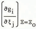is a N × M matrix, which is denoted A.

The equations:

are linear in ΔΞ and the best estimate for ΔΞ, ΔΞ is found by minimizing [ Y—G(Ξ_o) – AΔΞ] (Reference Whittaker and RobinsonWhittaker and Robinson 1967; Remmer 1972):

The best estimate for the elements, Ξ_E is thus:

If the first order terms ΔΞ_E are large, e.g. greater than the standard deviations of the estimates, the process is repeated by chosing the estimate Ξ_E as the new Ξ_o. In this way the process is iterative.

The least squares method also provides estimates of the variances:

where I_NN is a N × N unit matrix, D_E = Y—G(Ξ_o)—AΔΞ_E is a N – dimensional vector representing the best estimate of the residual vector D, Y_E = Y–D_E is the best estimate of E(Y) and s is the best estimate of the standard deviation σ.

If the model (2) succeeds in describing the motion of the characteristic point, P, on the glacier surface, the estimate of the standard deviation on the directional observations, s, should be of the same order of magnitude as the measuring accuracy of these. If the model does not succeed, the model can be changed. Care must be taken in adding new elements to the model, as extra elements may result in a decreased deviation, s (Reference LindgrenLindgren 1976), but the new elements need not necessarily have statistical significance. As an approximate rule, adding an element should reduce s² by at least 5%.

Demonstration

The method is used on data from the Daugaard-Jensen Glacier in East Greenland (7I°N, 28 °W). This 66 km long outlet glacier terminates in Nordvest Fjorden with a 90 m vertical front (Reference Reeh and OlesenReeh and Olesen 1968; Reference Olesen and Reeh1969; Reference Reeh and Olesen1986). The theodolite measurements are made to characteristic points on the glacier surface in the terminus area, where the glacier moves about 10 m/day. The observation series used here cover a time span of 4 – 10 days and each characteristic point on the glacier surface is represented by 4 – 17 independent directional observations from each fixed point (Reeh and Olesen 1968).

In this demonstration, 13 points, with relatively many observations, are chosen (N > 16). The model (2) is applied to each of the 13 points. The iterative process of equation (9) was very efficient, never requiring more than 7 iterations, even with poor start values of Ξ_o. The model never failed to converge. The calculated positions and velocities are shown in Fig.2. Table 1 contains a list of the elements of the 4 points (c, h, k and m) with most observations. The positions (x_o,y_o,z_o) of the points at the time t_o are determined with a standard deviation, in the horizontal direction, of the order of I m, and, in the vertical direction, of the order of 0.1 m. The standard deviations in the ê_x–direction are generally two times the standard deviation in the ê_y–direction, because the bearings from the fixed points, A and B, are almost parallel to the ê_x–direction. The surface velocities are of the order of 10 m/day, with an accuracy of 0.1 m/day, and the flow directions are determined within 0.5 degrees. The best estimate of the standard deviation of the directional observations, especially for the 4 points listed in Table 1, are of the order of 20” (1·10⁻⁴ rad), which is greater than the measuring accuracy on the directional observations of 7” (0.34-10⁻⁴ rad) (Reeh, personal communication).

Table I

Best Estimates of the Model Parameters Ξ For the Four Points, c,h,k and m, From the Simple Model (2), and The Modified Model (11). The Estimated Standard Deviations on the Angle Observations s and The Numbers of Freedom N – M are also Shown.

Figure 3a shows the first n elements of the estimated residual vector, D_E, for the four points: c, h, k and m, representing the measuring errors on the angles α. The deviations are systematic, suggesting a modification of the simple model (2).

Fig. 3.

The best estimates of the first n elements of the residual vector D, D_E, for the four points, c,h,k and m, corresponding to the estimated measuring error on the angles α from fixed point A. Fig.3a shows the estimates from the simple model (2), and Fig.3b the estimates from the modified model (11).

In the modified model a harmonic component is added to the velocity term:

which increases the number of elements to be estimated to M = 10:

The least-squares method is used, and the estimates are presented in Table 1.

The estimated positions, velocities and accelerations are very similar to the first estimates, but the standard deviations have been reduced. The “new” elements, V₁ and V₂, represent an amplitude of the order of 0.32 m/day, and an angular frequency of the order 1 (day)⁻¹ (wavelength ≈ 6.5 days) for all four points. The standard deviations of the amplitude are of the same order of magnitude as the standard deviation of the velocity, v_Q. The estimated standard deviations on the directional observations, s, are reduced by 30%, and the elements of the residual vector, D_E, for the α—angles (Fig.3b), are also reduced. Most of the systematic deviations have thus been reduced to the accuracy of the directional observations by adding the harmonic term to the original model.

The time-dependent velocity pattern is similar for all four points analysed, suggesting that this pattern applies for the whole glacier front.

Conclusion

The statistical method, described here, is based on a physical model, directly containing the parameters to be determined. A least squares method is used to calculate the best estimates of the model parameters from the directional observations, made with theodolite from two fixed points.

In the case of fast moving glaciers, where (he characteristic points on the glacier surface are observed in short periods of time, a simple model is described, where the points are assumed to move along straight lines.

As an advantage of the statistical method used here, the observations from the two fixed points need not necessarily be simultaneous, because the intermediate step of determining positions from each set of observations is omitted.

The demonstration of the method on the data from the Daugaard-Jensen glacier is successful. The position and velocities of the observed characteristic points on the glacier front are described basically within the standard deviations of the directional observations.

Other glaciers may require different models to describe the motion of the observed points. The statistical method can also be applied to cases where, e.g., strain rates, or external observations, such as hours of sunshine, basal water pressure, etc., are included in the model.