1 Introduction
The study of grid turbulence has been of interest for decades. Regular grids made of bars with uniform mesh size have been used by many to study homogeneous/isotropic turbulence (e.g. Comte-Bellot & Corrsin Reference Comte-Bellot and Corrsin1966, Reference Comte-Bellot and Corrsin1971; Gad-El-Hak & Corrsin Reference Gad-El-Hak and Corrsin1974; Mohamed & Larue Reference Mohamed and Larue1990; Mydlarski & Warhaft Reference Mydlarski and Warhaft1996; Cardesa, Nickels & Dawson Reference Cardesa, Nickels and Dawson2012). Other efforts have also been made to develop different types of devices to produce shear flows in wind tunnel experiments. Some of the most popular methods are briefly reviewed here, and reviews of the earlier methods can be found in Lawson (Reference Lawson1968) and Laws & Livesey (Reference Laws and Livesey1978). Here and for the rest of the discussion,
 $x$
,
 $y$
,
 $z$
represent the streamwise, vertical and transverse direction, respectively.
1.1 Shear generating methods
Several methods have been proposed to generate shear flows in laboratories. One of the methods is to use wire gauzes to modify the local solidity, and consequently produce a mean velocity gradient. The effect of flow passing through wire gauzes was described in detail by Taylor et al. (Reference Taylor, Batchelor, Dryden and Schubauer1949). Then by using resistance and deflection coefficients as grid properties, a theoretical method of grid design was offered by Owen & Zienkiewicz (Reference Owen and Zienkiewicz1957) relating the downstream mean velocity profile to the spacing of the wires, and a uniform shear flow was produced in their study using parallel wires of diameter
 $d=3.175~\text{mm}$
. This theory was further generalized by Elder (Reference Elder1959) to non-uniform gauze with arbitrary shapes. Elder (Reference Elder1959) tested his theory on linear and parabolic gauzes, and proposed a gauze shape to generate a linear shear flow. Rose (Reference Rose1966) followed the same method and showed that the shape of the generated downstream mean velocity profile was persistent. The later studies of Livesey & Laws (Reference Livesey and Laws1973a
) on flow through curved gauze screens proposed a modification of the theory to exclude a higher-order term, which seemed to cause discrepancies between theoretical solutions and experimental data from two-dimensional and axisymmetric cases. Livesey & Laws (Reference Livesey and Laws1973b
) also produced axisymmetric velocity profiles using these curved screens. Dunn & Tavoularis (Reference Dunn and Tavoularis2007) revisited this type of method to combine theoretical and empirical information to produce shear flows through curved screens. Mean flows with approximately uniform shears and different shear rates were successfully generated in a water channel. The most obvious drawback of any method using gauze and wires is, as commented by Lawson (Reference Lawson1968), that the turbulence characteristics cannot be varied once the wire is chosen, and it is therefore impossible to generate mean velocity and turbulence profiles independently.
The parallel wire method relies mostly on the spacing of the wires, and it is therefore hard to adjust the elements locally. Another type of shear generator was tested by Champagne, Harris & Corrsin (Reference Champagne, Harris and Corrsin1970), where the authors used plates of 609.6 mm long, and 3.175 mm thick separated by 25.4 mm to form parallel channels with adjustable internal screens to control the local solidity. The same method was then used by many, e.g. Harris, Graham & Corrsin (Reference Harris, Graham and Corrsin1977); Tavoularis & Corrsin (Reference Tavoularis and Corrsin1981), Karnik & Tavoularis (Reference Karnik and Tavoularis1987), Rohr et al. (Reference Rohr, Itsweire, Helland and Van Atta1988), Garg & Warhaft (Reference Garg and Warhaft1998), Nedić & Tavoularis (Reference Nedić and Tavoularis2016), with different configurations such as the size of internal grid size, and the separation distance of the plates. A honeycomb with uniform cell diameter but varying lengths in the streamwise direction was also tested by Rose (Reference Rose1970) to generate shear flows. This author studied the combination of such a honeycomb and a grid placed downstream with different sizes and geometries, and the downstream grid was shown to reduce the mean shear rate. Richards & Morton (Reference Richards and Morton1976) produced a quadratic mean velocity profile using such a honeycomb and grid combination. Mulhearn & Luxton (Reference Mulhearn and Luxton1975) used a similar set-up where a non-uniform parallel rod grid was placed upstream of the honeycomb with uniform length to produce a uniform sheared flow. Note that no relation between the shear flow and the geometry of the set-up was concluded from these parallel plate methods since all of them were tuned by trial and error. Even though they offer the possibility of local adjustments of the device, which is an improvement of the previous method, they lack theoretical support to relate the grid geometry to the generated shear flow. Experiments involving extremely high shear rates, e.g.
 $\unicode[STIX]{x2202}U/\unicode[STIX]{x2202}y>400~\text{s}^{-1}$
(where
 $U$
is the mean velocity and
 $y$
is the shear direction, see Souza, Nguyen & Tavoularis Reference de Souza, Nguyen and Tavoularis1995), are excluded from our discussion. We also mention that there have been studies on the Couette flow generated by moving walls as a means to produce velocity profiles (Coles Reference Coles1965; Tillmark & Alfredsson Reference Tillmark and Alfredsson1992; Bottin et al.
Reference Bottin, Dauchot, Daviaud and Manneville1998), yet the fundamental idea is different from this study, and the discussion on these studies is therefore not elaborated here.
The active grid proposed by Makita (Reference Makita1991) and the subsequent works (see e.g. Mydlarski & Warhaft Reference Mydlarski and Warhaft1996; Shen & Warhaft Reference Shen and Warhaft2000; Cekli & van de Water Reference Cekli and van de Water2010; Knebel, Kittel & Peinke Reference Knebel, Kittel and Peinke2011; Hearst & Ganapathisubramani Reference Hearst and Ganapathisubramani2017) provided another option to tailor turbulent flows. It is typically used to produce a higher turbulence level, and is sometimes combined with other passive devices to produce shear flows (see e.g. Zhu et al.
Reference Zhu, van Hout, Luznik, Kang, Katz and Meneveau2006; Bai, Meneveau & Katz Reference Bai, Meneveau and Katz2012; Thormann & Meneveau Reference Thormann and Meneveau2015). Hearst & Ganapathisubramani (Reference Hearst and Ganapathisubramani2017) proposed the possibility to obtain independent control of the mean flow and turbulence intensity using the active grid. They produced shear flows with small shear rates ranging approximately
 $6.25$
–
 $12.5~\text{s}^{-1}$
over a physical domain of 0.32 m and generated profiles of varying turbulence intensity and high Reynolds numbers. Hearst & Ganapathisubramani (Reference Hearst and Ganapathisubramani2017) claimed that such shear flows would be directly applicable in wind turbine experiments. Amongst many advantages, the methodology of active grid-generated turbulence, however, is rather costly to implement, and the establishment of control protocols is largely empirical. The work of Hearst & Ganapathisubramani (Reference Hearst and Ganapathisubramani2017) did not provide quantitative relations between the control parameters and the turbulence characteristics. Therefore we explore the possibility of a type of passive grid design for producing desired turbulence fields. This idea is also supported by the conclusion of Roach (Reference Roach1987) that the turbulence energy scales on the bar dimensions rather than the mesh size, which suggests that it is possible to manipulate the turbulence intensity through the design of the grid bars.
In this paper we attempt to combine the known methodology for producing mean shear with fractal/multiscale ways to produce scalable high turbulence intensities at the same time. For this reason, we refer to the studies of fractal grids proposed by Hurst & Vassilicos (Reference Hurst and Vassilicos2007), especially the space filling fractal square grids (e.g. Seoud & Vassilicos Reference Seoud and Vassilicos2007; Mazellier & Vassilicos Reference Mazellier and Vassilicos2010; Valente & Vassilicos Reference Valente and Vassilicos2011; Gomes-Fernandes, Ganapathisubramani & Vassilicos Reference Gomes-Fernandes, Ganapathisubramani and Vassilicos2012; Hearst & Lavoie Reference Hearst and Lavoie2014; Isaza, Salazar & Warhaft Reference Isaza, Salazar and Warhaft2014) where the development of downstream turbulence is quantitatively related to the grid geometries. These fractal square grids are characterized by repeated square patterns of different sizes, and the blockage ratio is usually small (
 $\unicode[STIX]{x1D70E}\approx 25$
–
 $30\,\%$
). Detailed descriptions can be found in Seoud & Vassilicos (Reference Seoud and Vassilicos2007), Hurst & Vassilicos (Reference Hurst and Vassilicos2007), Mazellier & Vassilicos (Reference Mazellier and Vassilicos2010).
Mazellier & Vassilicos (Reference Mazellier and Vassilicos2010) studied the fractal-generated turbulence, and proposed the wake interaction length scale
 $x_{\ast }=g_{0}^{2}/w_{0}$
, where
 $g_{0}$
is the largest length of the bars, and
 $w_{0}$
is the largest width. This scaling relation succeeded in collapsing both the centreline mean velocity and turbulence intensity profiles. The peak of the turbulence intensity was found at
 $x_{peak}\approx 0.45x_{\ast }$
with a maximum level of approximately 15 %
 $U_{\infty }$
. Later, Gomes-Fernandes et al. (Reference Gomes-Fernandes, Ganapathisubramani and Vassilicos2012) extended the study to include the effects of the aspect ratio of the bars and the free-stream turbulence level, and proposed the improved scaling relation
 $x_{\ast }^{peak}=0.21g_{0}^{2}/(\unicode[STIX]{x1D6FC}C_{D}w_{0})$
, where
 $\unicode[STIX]{x1D6FC}=0.231$
is a constant associated with the wake development for flows with minimal inlet free-stream turbulence intensity, and
 $C_{D}$
is the drag coefficient of the bar. This
 $x_{\ast }^{peak}$
provided better collapse of the streamwise turbulence intensity profiles from different grids, and was taken to be an important parameter for designing the grids. Gomes-Fernandes et al. (Reference Gomes-Fernandes, Ganapathisubramani and Vassilicos2012) also proposed a scaling relation for the turbulence intensity levels, and the scaled turbulence intensity
 $(u^{\prime }/U_{\infty })\unicode[STIX]{x1D6FD}(C_{D}w_{0}/x_{\ast }^{peak})^{-1/2}$
(where
 $\unicode[STIX]{x1D6FD}=2.88$
is a constant for laminar free stream, and
 $U_{\infty }$
is the inlet free-stream velocity) collapsed six different inlet conditions as a function of
 $x/x_{\ast }^{peak}$
. These scalings are adapted and discussed further in the design process of our new multiscale inhomogeneous grids.
1.2 Shear flow characteristics
The development of turbulence intensity in a grid-generated shear flow was perhaps first discussed by Rose (Reference Rose1966). The author generated a homogeneous turbulent shear flow with a mean shear gradient
 $S=\unicode[STIX]{x2202}U/\unicode[STIX]{x2202}y=13.69~\text{s}^{-1}$
which retained its value up to
 $x/H=9.76$
, where
 $H$
is the height of the grid. The turbulence intensities
 $u^{\prime }$
and
 $v^{\prime }$
were found to be nearly uniform along the mean shear direction
 $y$
at
 $x/H=1.33$
, but the two edges were affected by the growing boundary layer on the tunnel wall and the turbulent intensities were significantly larger on the sides. Along the centreline,
 $u^{\prime }$
and
 $v^{\prime }$
decayed to levels
 $u^{\prime }/U_{c}=1.2\,\%$
and
 $v^{\prime }/U_{c}=0.8\,\%$
, where
 $U_{c}$
is the centreline mean streamwise velocity.
Champagne et al. (Reference Champagne, Harris and Corrsin1970) produced a mean shear rate
 $S=12.9~\text{s}^{-1}$
using the parallel plates with internal screens, and the shear was maintained in the range
 $x/H=3{-}9.5$
. The centreline turbulence intensity
 $u^{\prime }/U_{c}$
reached a constant value of 1.8 % after
 $x/H=6.5$
. Rose (Reference Rose1970) created shear flows using different combinations of honeycomb and wire grids, and produced mean shear rates in the range
 $S=6$
–
 $12~\text{s}^{-1}$
. The streamwise turbulence intensity levels
 $u^{\prime }/U_{c}$
in the range
 $x/H=7{-}9$
were shown to be constant, and their values increased from 0.2 to 2 % with increasing grid size.
Harris et al. (Reference Harris, Graham and Corrsin1977) improved on the work of Champagne et al. (Reference Champagne, Harris and Corrsin1970) and produced a larger mean shear rate
 $S=44~\text{s}^{-1}$
which remained almost constant up to a dimensionless time scale
 $\unicode[STIX]{x1D70F}^{\ast }=12$
, where
 $\unicode[STIX]{x1D70F}^{\ast }\equiv (x/U_{c})(\unicode[STIX]{x2202}U/\unicode[STIX]{x2202}y)$
. Their hot-wire results showed a larger normalized turbulence intensity compared to that in Champagne et al. (Reference Champagne, Harris and Corrsin1970), and the turbulence intensities were found to grow with streamwise distance after
 $\unicode[STIX]{x1D70F}^{\ast }\approx 4$
. The growth of turbulence intensities along the streamwise direction was then studied by Rohr et al. (Reference Rohr, Itsweire, Helland and Van Atta1988) for several cases, where the grid size, centreline velocity and mean shear rate were varied. The results clearly showed a region of increasing streamwise turbulence intensity
 $u^{\prime }/U_{c}$
. The critical point
 $\unicode[STIX]{x1D70F}_{c}^{\ast }$
, where
 $u^{\prime }/U_{c}$
reached its minimum was studied by several authors, and interestingly the turbulence intensity beyond
 $\unicode[STIX]{x1D70F}_{c}^{\ast }$
remained constant in some cases (e.g. Rose Reference Rose1966; Champagne et al.
Reference Champagne, Harris and Corrsin1970; Rose Reference Rose1970), but grew in some others (e.g. Harris et al.
Reference Harris, Graham and Corrsin1977; Tavoularis & Corrsin Reference Tavoularis and Corrsin1981; Rohr et al.
Reference Rohr, Itsweire, Helland and Van Atta1988; Nedić & Tavoularis Reference Nedić and Tavoularis2016). For the cases where
 $u^{\prime }/U_{c}$
stayed constant, the development was fairly fast, reaching constant values at
 $\unicode[STIX]{x1D70F}_{c}^{\ast }=1.6$
–
 $3$
, whereas for those cases exhibiting growing
 $u^{\prime }/U_{c}$
the critical point was observed at roughly
 $\unicode[STIX]{x1D70F}_{c}^{\ast }=4$
–
 $5$
. Tavoularis & Karnik (Reference Tavoularis and Karnik1989) studied this more systematically and suggested that when the shear is weak, i.e.
 $\unicode[STIX]{x1D716}/P\sim 1$
, the turbulence kinetic energy will remain constant after
 $\unicode[STIX]{x1D70F}_{c}^{\ast }$
, whereas for strong shears, where
 $\unicode[STIX]{x1D716}/P<1$
, the turbulence kinetic energy will grow exponentially after
 $\unicode[STIX]{x1D70F}_{c}^{\ast }$
.
Regarding the Taylor microscale
 $\unicode[STIX]{x1D706}$
, Harris et al. (Reference Harris, Graham and Corrsin1977) reported a constant value of
 $\unicode[STIX]{x1D706}$
in the range
 $\unicode[STIX]{x1D70F}^{\ast }=6{-}11$
, with
 $S=44~\text{s}^{-1}$
. Rohr et al. (Reference Rohr, Itsweire, Helland and Van Atta1988) also reported a constant
 $\unicode[STIX]{x1D706}$
from
 $\unicode[STIX]{x1D70F}^{\ast }=6$
with approximately
 $S=1~\text{s}^{-1}$
, while Tavoularis & Karnik (Reference Tavoularis and Karnik1989) showed in their experiments that
 $\unicode[STIX]{x1D706}$
approached a constant value at
 $\unicode[STIX]{x1D70F}^{\ast }\approx 16$
for mean shear rates
 $S=44~\text{s}^{-1}$
and
 $84~\text{s}^{-1}$
. More recently Nedić & Tavoularis (Reference Nedić and Tavoularis2016) reported a constant
 $\unicode[STIX]{x1D706}$
downstream of
 $\unicode[STIX]{x1D70F}^{\ast }\approx 9.25$
in a uniformly sheared flow with
 $S=62~\text{s}^{-1}$
. By comparing the results from Harris et al. (Reference Harris, Graham and Corrsin1977) and Rohr et al. (Reference Rohr, Itsweire, Helland and Van Atta1988), it can be concluded that the location where
 $\unicode[STIX]{x1D706}$
stops growing is not only a function of the mean shear rate, but other factors as well.
In terms of integral length scales, all of the previous results showed monotonic increases with streamwise distance. Results by Nedić & Tavoularis (Reference Nedić and Tavoularis2016) also showed a decrease of growth rate of the longitudinal integral length scale
 $L_{uu,x}$
beyond approximately
 $\unicode[STIX]{x1D70F}^{\ast }=9$
. Some studies reported relations between longitudinal and transverse integral length scales such that
 $L_{uu,x}=2L_{uu,y}$
, indicating a large scale isotropy (e.g. Rose Reference Rose1966; Champagne et al.
Reference Champagne, Harris and Corrsin1970; Harris et al.
Reference Harris, Graham and Corrsin1977). Further discussion on length scales is provided in § 3.5.1.
1.3 Objectives
The main objective of the present work is to design and test a new class of turbulence generating grids to find the possibility to scale the mean velocity and turbulence intensity profiles to the geometry of the grid, which might provide the ability to produce desired mean velocity and near-field turbulence intensity profiles simultaneously. For the current discussion, only weakly sheared turbulence is considered with shear rates ranging from
 $0$
to
 $5~\text{s}^{-1}$
, comparable to the cases studied by Hearst & Ganapathisubramani (Reference Hearst and Ganapathisubramani2017) using active grids. Such weakly sheared flows can be used to represent a certain part of a shear layer, and therefore are practical in various wind tunnel testing scenarios. Even though homogeneous shear flows are important as a subject of fundamental interest, they are not the subject of the present study. In this paper, we attempt to establish relations between the geometry and different turbulent flow profiles. Homogeneous turbulent shear flows could be considered in a future study, which might attempt to apply our method of flow generation.
In the following context, the details of the grid geometry are given first. It is then shown that the mean velocity profiles predicted using the mean velocity model derived from Taylor et al. (Reference Taylor, Batchelor, Dryden and Schubauer1949) and McCarthy (Reference McCarthy1964) are in good agreement with our experimental data. By modifying the grid thickness the aspect ratio of the grid bars are changed, and consequently the drag coefficients. The effect of drag coefficient on the local mean velocity gradient is discussed. The turbulence intensity profiles at given streamwise location
 $x$
are found to scale with the geometry of the grid bars. The scaling relations between the turbulence field and the geometry of the grid might be used in the future to generate other types of turbulence flows of interest. A general procedure of the grid design method is proposed in § 3.3.
Results on the evolution of turbulence intensities and length scales are also presented, and finally a simplified model is proposed to describe the downstream development of the turbulence field generated by these grids. This model allows description of the turbulence field using just one measurement of vertical profile close to the grid and one centreline profile along the streamwise direction.
2 Experiments
2.1 Facility
All experiments were conducted in the
 $3^{\prime }\times 3^{\prime }$
closed loop wind tunnel in the Aeronautics Department at Imperial College London. The test section has a cross-sectional area of
 $0.91\times 0.91~\text{m}$
, and a measurable length of 4.2 m. The flow goes through a set of perforated screens and a 9:1 contraction before reaching the test section. The background turbulence intensity without the grid was measured to be
 ${\sim}0.1\,\%$
at
 $U_{\infty }=10~\text{ms}^{-1}$
. A computer controlled traversing system is mounted on top of the working section, allowing movements in all three directions. The origin of the coordinate system is set at the bottom of the grid on the windward side.
2.2 Grid design
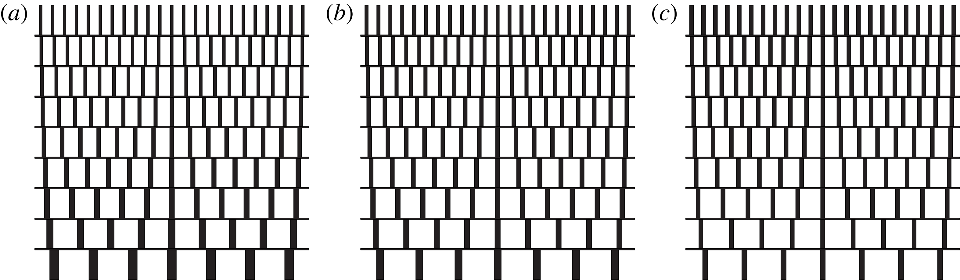
In this section we outline the design principles of our new multiscale grids. A schematic sketch is given in figure 1. Three such grids were made for the current investigation producing flows with different shear rates and different turbulence profiles, even though the geometries are very similar. The first grid was designed to generate a turbulent flow without mean shear, and a non-uniform turbulence intensity, while the other two were designed to generate turbulent flows with gradients in both mean velocity and turbulence intensity. The grids are numbered in order of increasing shear rates. They were laser cut in acrylic with a uniform thickness (in the
 $x$
direction) of
 $D=10~\text{mm}$
.
Schematic sketch of (a) grid 1, (b) grid 2 and (c) grid 3, respectively, in the
 $z$
–
 $y$
(horizontal–vertical) plane with
 $N=9$
layers numbered from bottom to top as
 $n=1,2,\ldots ,N$
.

Design parameters of multiscale shear grids.
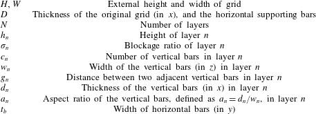
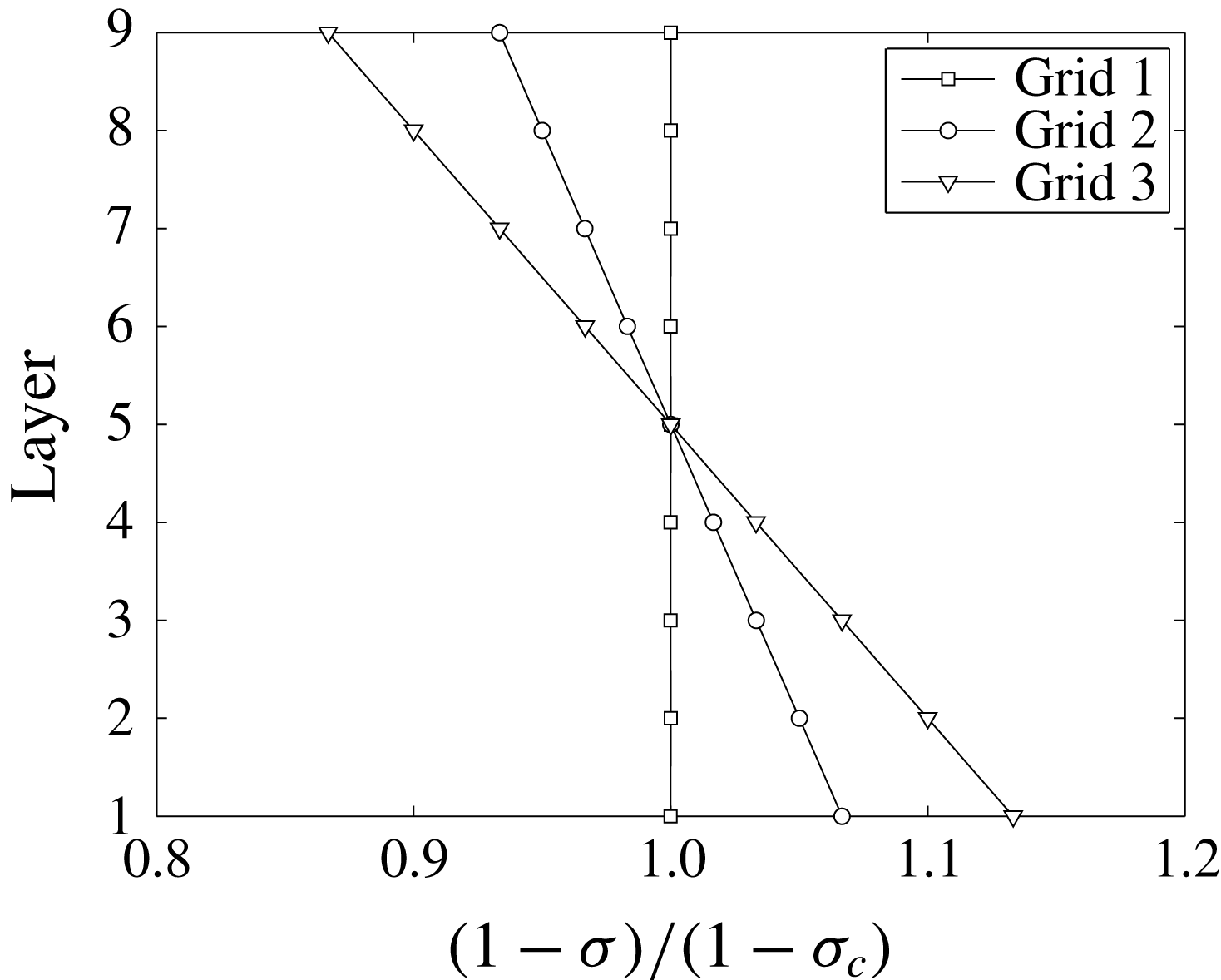
Profiles of
 $(1-\unicode[STIX]{x1D70E})/(1-\unicode[STIX]{x1D70E}_{c})$
for grid 1, 2 and 3, where
 $\unicode[STIX]{x1D70E}_{c}$
is the blockage ratio at layer 5, the centre of the grid, i.e.
 $\unicode[STIX]{x1D70E}_{c}=\unicode[STIX]{x1D70E}_{5}$
.
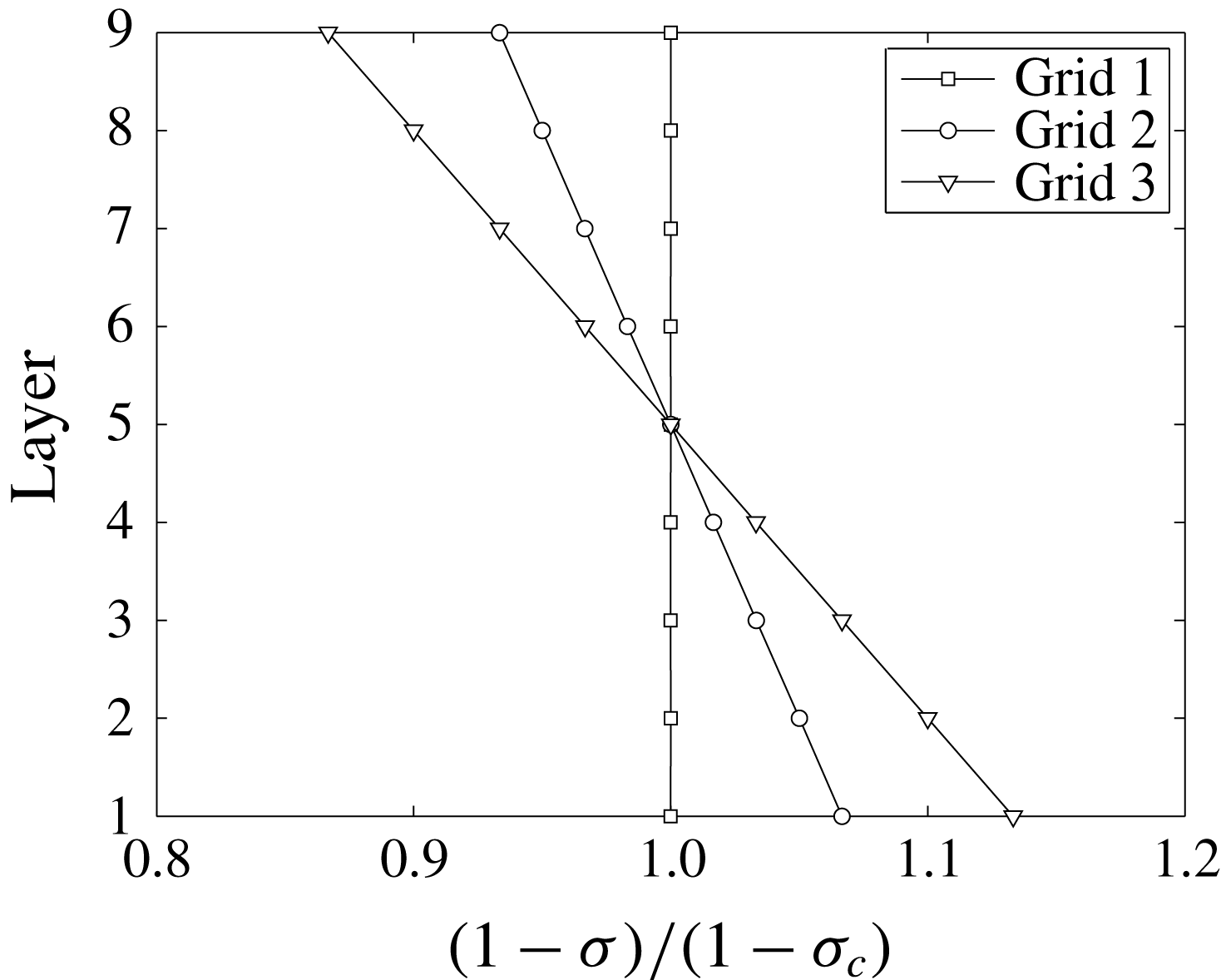
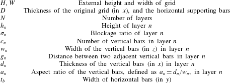
There are several parameters involved in the design process, and a summary is given in table 1. The external height
 $H$
and width
 $W$
of the grid are determined by the dimensions of the wind tunnel test section in the
 $y$
and
 $z$
directions, respectively. For the current study we have
 $H=W=0.91~\text{m}$
. The number
 $N$
of horizontal layers is chosen to be
 $N=9$
for all three grids in the current study. This number can be increased to obtain finer control over the local velocity gradient. The height of each layer
 $h_{n}$
is set here to be
 $h_{n}=\text{constant}=101.67~\text{mm}$
. There are also eight horizontal supporting bars. Their width (in the
 $y$
direction) for the present grids is
 $t_{b}=5~\text{mm}$
, and an aspect ratio of
 $D/t_{b}=2$
was achieved to minimize the wake shed from them.
The most important parameters for the design of the mean flow profile are the blockage ratios
 $\unicode[STIX]{x1D70E}_{n}$
of each layer. The normalized blockage ratio profiles for each grid are given in figure 2. The mean blockage ratio
 $(\unicode[STIX]{x1D70E}_{1}+\unicode[STIX]{x1D70E}_{2}+\cdots +\unicode[STIX]{x1D70E}_{n})/N$
(with
 $N=9$
here) was set to 25 % for all three grids, while the maximum local blockage ratio was set as
 $\unicode[STIX]{x1D70E}_{9}=\unicode[STIX]{x1D70E}_{max}=35\,\%$
to avoid flow recirculation. This is consistent with the observations of Rose (Reference Rose1966), who limited the maximum local solidity to
 $\unicode[STIX]{x1D70E}_{max}=40\,\%$
for this reason.
While the blockage profile controls the mean velocity of the flow, the lateral widths and spacing of the vertical bars in each layer of the grid are tailored to vary the wake interaction mechanisms in order to generate different turbulence characteristics. Three parameters are introduced here, namely
 $c_{n}$
the number of vertical bars,
 $w_{n}$
the lateral width of each individual bar and
 $a_{n}$
the aspect ratio of the bars (defined as
 $a_{n}=d_{n}/w_{n}$
). Note that since the thickness of the original grid is constant, i.e.
 $d_{n}=D=10~\text{mm}$
,
 $a_{n}$
varies with vertical bar width
 $w_{n}$
and the drag coefficient
 $C_{D}$
of each bar therefore varies with
 $n$
, which affects the wake characteristics. The number of bars for each layer is set to be
 $c_{n}=2(n+M)+1$
for
 $n=1,2,\ldots ,N$
, where
 $M=2$
is a control parameter for the current grids. The width of the bars are calculated from
 $$\begin{eqnarray}\displaystyle w_{n}=\left\{\begin{array}{@{}ll@{}}{\displaystyle \frac{W}{c_{n}}}\left({\displaystyle \frac{h_{n}\unicode[STIX]{x1D70E}_{n}-t_{b}}{h_{n}-t_{b}}}\right), & n=2,3,\ldots ,N-1\\ {\displaystyle \frac{W}{c_{n}}}\left({\displaystyle \frac{h_{n}\unicode[STIX]{x1D70E}_{n}-0.5t_{b}}{h_{n}-0.5t_{b}}}\right), & n=1,N.\end{array}\right. & & \displaystyle\end{eqnarray}$$
As shown in figure 1, there are no horizontal bars at the top and bottom edges of the grids, and the area is distributed in the vertical bars at layer 1 and
 $N$
using the second equation in (2.1). At each layer, the vertical bars are evenly separated by a distance
 $g_{n}$
, and are placed symmetrically about
 $z=0$
.
Note that the uniform thickness of the original grid inevitably causes variable aspect ratios
 $a_{n}=d_{n}/w_{n}$
of the vertical bars as the width
 $w_{n}$
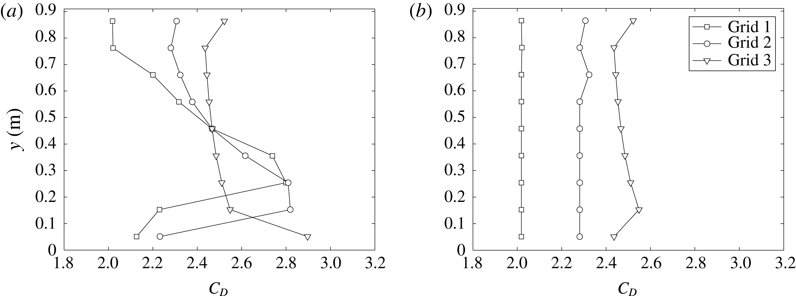
varies. Figure 3(a) gives the
 $C_{D}$
profiles of the three grids evaluated using the relation between
 $C_{D}$
and the aspect ratio
 $a_{n}$
given by Bearman & Trueman (Reference Bearman and Trueman1972). The Reynolds number of the vertical bars with
 $U_{\infty }=10~\text{ms}^{-1}$
is within the range 6000–20 000, and the Reynolds number dependence of the drag coefficient
 $C_{D}$
is therefore negligible. The grids were also modified by attaching blocks behind the vertical bars to achieve a uniform aspect ratio
 $a_{n}$
by effectively varying
 $d_{n}$
, and hence a uniform
 $C_{D}$
. Due to the dimensions of the vertical bars, the aspect ratio is set equal to that of the eighth layer
 $a_{8}$
. For grid 3, however, the modification was only applied to the bottom layer
 $n=1$
, because the additional thicknesses to be attached to the other layers were all smaller than 1 mm, and therefore difficult to manufacture. The drag coefficient profiles after the modification are given in figure 3(b).
Vertical drag coefficient profiles of (a) original grids with uniform thickness
 $D=10~\text{mm}$
, and (b) modified grids with variable thickness but uniform aspect ratio.

Now if we refer to the scalings for grid-generated turbulence proposed by Vassilicos and colleagues as outlined in the introduction, we can calculate the wake interaction length scale for each layer
 $n$
as
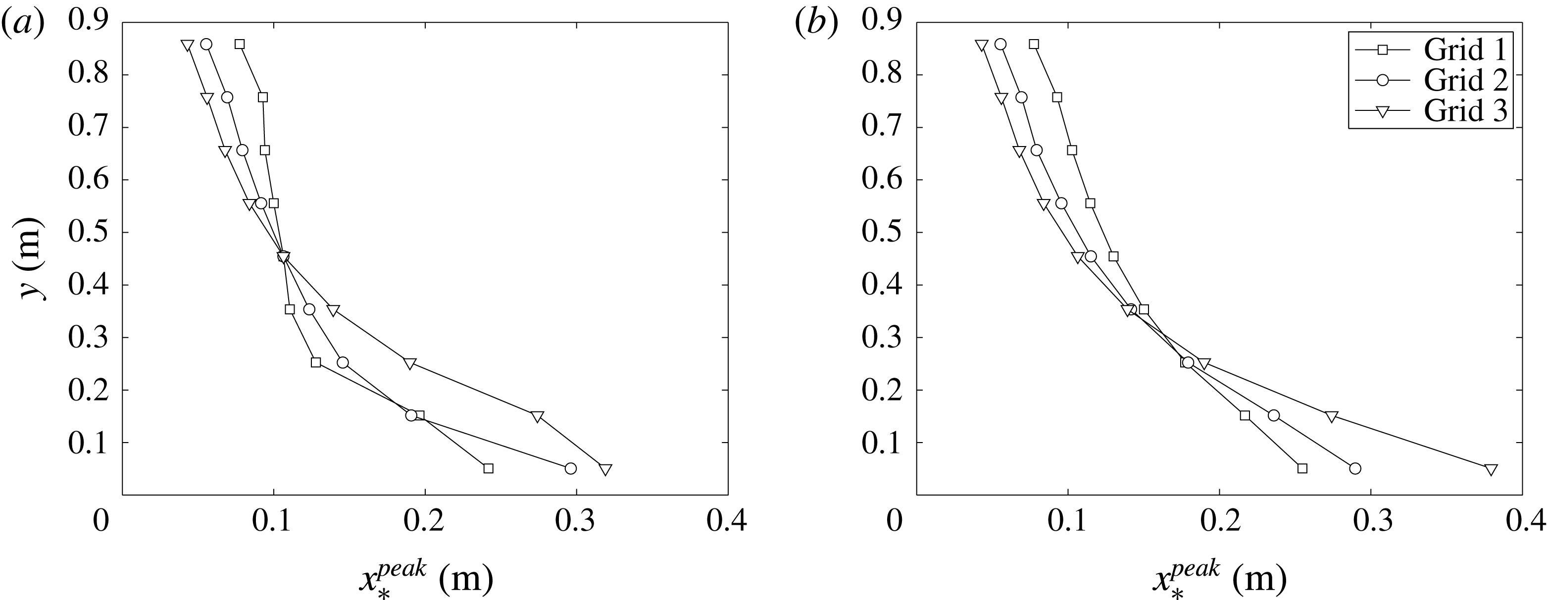
 $x_{\ast ,n}^{peak}=0.21g_{n}^{2}/(\unicode[STIX]{x1D6FC}C_{D}w_{n})$
by substituting
 $L_{0}=g_{n}$
and
 $t_{0}=w_{n}$
in their original equation (Gomes-Fernandes et al.
Reference Gomes-Fernandes, Ganapathisubramani and Vassilicos2012). The results for the original and modified grids are plotted in figure 4(a,b), respectively. It can be observed that the variation of
 $x_{\ast ,n}^{peak}$
with
 $n$
becomes much more smooth due to the modification of
 $C_{D}$
, and the maximum
 $x_{\ast }^{peak}$
is approximately
 $x=0.38~\text{m}$
from the grid. From the results of Gomes-Fernandes et al. (Reference Gomes-Fernandes, Ganapathisubramani and Vassilicos2012), where the turbulence intensity profiles from several experiments and different grids collapsed against
 $x/x_{\ast }^{peak}$
, it can be expected (see Gomes-Fernandes et al.
Reference Gomes-Fernandes, Ganapathisubramani and Vassilicos2012) that the streamwise turbulence intensity at level
 $n$
scales with
 $(x_{\ast }^{peak})^{1/2}$
. Further results and discussions on this scaling relation are presented in § 3.2.
The wake interaction length scale
 $x_{\ast ,n}^{peak}$
for (a) original grids with uniform thickness
 $D=10~\text{mm}$
, and (b) modified grids with variable thickness but uniform aspect ratio.

2.3 Experimental set-up and method
The tunnel inlet velocity
 $U_{\infty }$
was monitored using a Furness Controls FCO510 micromanometer which measures the static pressure head across the contraction and the temperature. The inlet velocity
 $U_{\infty }$
was maintained using a proportional–integral–derivative (PID) controller to be within
 $\pm 1.5\,\%$
of
 $10~\text{m}~\text{s}^{-1}$
for all data sets in the current study. Only one inlet velocity is tested as previous studies showed that the turbulence statistics produced by grid with square bars is independent of the Reynolds number (see Roach Reference Roach1987). Data were then acquired with MATLAB, using a 16-Bit National Instruments NI-6229(USB) board. Instantaneous velocity signals were measured using an in-house etched platinum Wollaston cross-wire powered by a Dantec Streamline CTA system. The diameter of the wire was
 $d_{w}=5~\unicode[STIX]{x03BC}\text{m}$
with length to diameter ratio approximately
 $200$
. Resolution of the wire are estimated to be
 $l/\unicode[STIX]{x1D702}=2.6{-}7.2$
, where the Kolmogorov length scale
 $\unicode[STIX]{x1D702}$
was estimated using
 $\unicode[STIX]{x1D702}=(\unicode[STIX]{x1D708}^{3}/\unicode[STIX]{x1D716})^{1/4}$
. To calculate
 $\unicode[STIX]{x1D716}$
, we compute
 $\unicode[STIX]{x1D716}_{\ast }=15\unicode[STIX]{x1D708}\overline{(\unicode[STIX]{x2202}u/\unicode[STIX]{x2202}x)^{2}}$
and
 $\unicode[STIX]{x1D716}_{\ast \ast }=3\unicode[STIX]{x1D708}\overline{(\unicode[STIX]{x2202}u/\unicode[STIX]{x2202}x)^{2}}+6\unicode[STIX]{x1D708}\overline{(\unicode[STIX]{x2202}v/\unicode[STIX]{x2202}x)^{2}}$
, and then use the average
 $\unicode[STIX]{x1D716}=(\unicode[STIX]{x1D716}_{\ast }+\unicode[STIX]{x1D716}_{\ast \ast })/2$
in this paper.
The hot-wire probe was mounted on a servo motor to allow accurate control of the pitching angles. It was calibrated at the beginning and end of every data set acquired using the look-up table method for five velocities from
 $3$
to
 $19~\text{m}~\text{s}^{-1}$
and seven angles ranging from
 $-27^{\circ }$
to
 $27^{\circ }$
. The temperature was monitored during acquisitions, and the data were discarded if temperature variation
 $\unicode[STIX]{x0394}T_{a}=T_{a,max}-T_{a,min}$
was larger than
 $0.1\,^{\circ }\text{C}$
. Two packets of
 $t_{s}=300~\text{s}$
samples were acquired to ensure convergence in mean statistics. Longer samples (
 $t_{s}>300~\text{s}$
) were not possible as the drift of the ambient temperature during acquisition will add artificial large scale variation. The acquisition rate was 125 kHz, and a low-pass filter of 30 kHz was applied before the data were recorded to avoid aliasing. The data were also low-pass filtered before the processing to eliminate high frequency noise.
To calculate the longitudinal integral length scales
 $L_{uu,x}$
, one either integrates the correlation function
 $R_{uu}$
or uses the streamwise turbulence kinetic energy spectrum
 $E_{11}(k)$
as
 $L_{uu,x}=\unicode[STIX]{x03C0}E_{11}(0)/(2u^{\prime 2})$
(see Tennekes & Lumley Reference Tennekes and Lumley1972). It is noted that the spectrum and the correlation function is a Fourier pair. Yet the zero frequency asymptote of the digitally acquired spectrum has large uncertainty and the integral length scale is usually extrapolated from a number of the low frequency spectral estimates. For the other method, the integral of the correlation function cannot be taken to infinity, and thus an upper limit of the integration has to be chosen. Moreover, this upper limit of the integration is not well defined, and the integration result using different upper limit varies as large as
 $20\,\%$
(O’Neill et al.
Reference O’Neill, Nicolaides, Honnery and Soria2004). We therefore seek a way to correct the lower frequency range of the spectra before estimating the longitudinal integral length scale
 $L_{uu,x}$
.
Several models have been proposed for estimating the power spectra density
 $E(k)$
, and the most frequently used is the von Kármán model, which can be written in a one-dimensional form as
 $$\begin{eqnarray}\displaystyle E_{11}(k)=\frac{2u^{\prime 2}L_{uu,x}}{\unicode[STIX]{x03C0}}\frac{1}{\{1+[kL_{uu,x}B(1/2,1/3)/\unicode[STIX]{x03C0}]^{2}\}^{5/6}}, & & \displaystyle\end{eqnarray}$$
where
 $u^{\prime }$
is the turbulence intensity,
 $k$
is the wavenumber defined as
 $k=2\unicode[STIX]{x03C0}f/U_{\infty }$
(
 $f$
is the frequency in time) and
 $B$
is the beta function related to the
 $\unicode[STIX]{x1D6E4}$
function by
 $B(1/2,1/3)=\unicode[STIX]{x1D6E4}(1/2)\unicode[STIX]{x1D6E4}(1/3)/\unicode[STIX]{x1D6E4}(5/6)$
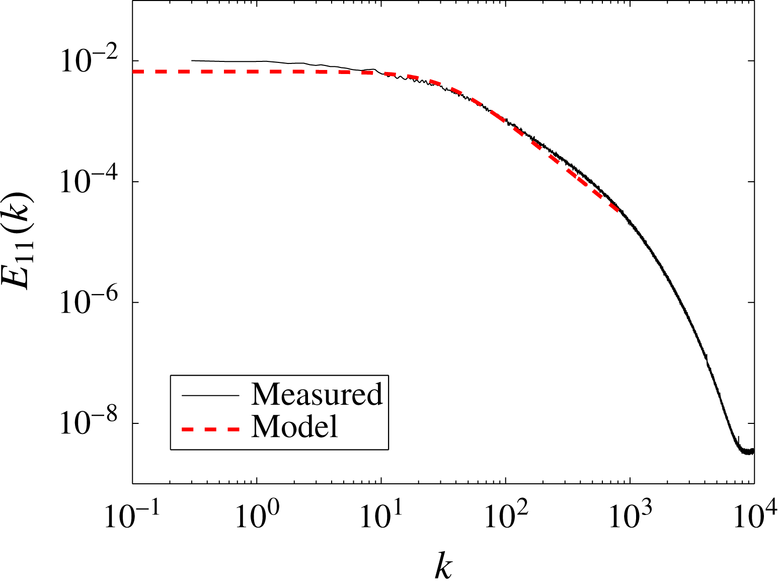
. In practice, we first take the average of the spectra of two packets of data, and use (2.2) to fit the data in a least square sense. One example is given in figure 5, where it is shown that the small wavenumber range of the original spectrum (black) is slightly tilted upward leading to a larger value of
 $E_{11}(0)$
. This effect is most obvious at locations close to the grid where
 $x=0.83~\text{m}$
, but much less further downstream. This method is used in § 3.5.1 to correct the lower frequency part of the spectrum.
It is acknowledged that most spectrum models have potential flaws in the low frequency range. There have been other models, e.g. Wilson (Reference Wilson1998), where a two parameter spectrum model is proposed that allows more freedom in fitting the inertial range and inertial sub-range of the spectrum. However, that model works well only in turbulent flows with sufficiently large Reynolds numbers that has more decades of
 $-5/3$
slope, otherwise the extra parameter causes large uncertainties in the fitted spectrum. For the current study, the Reynolds number is moderate so that models such as Wilson’s (Reference Wilson1998) are not considered.
Example spectrum for grid 2 at centreline
 $x=0.83~\text{m}$
.

3 Results
3.1 Mean velocity
Before showing the measured vertical mean velocity profiles produced by the grids, we refer to previous works that used wire gauzes to produce non-uniform mean flow profiles. Following Taylor et al. (Reference Taylor, Batchelor, Dryden and Schubauer1949), McCarthy (Reference McCarthy1964), the streamwise velocity near the grid (upstream denoted by ‘
 $-0$
’ and downstream denoted by ‘
 $+0$
’) can be related by
 $$\begin{eqnarray}\displaystyle \frac{U_{+0}}{U_{-0}}=\frac{1+\unicode[STIX]{x1D6FC}_{n}-\unicode[STIX]{x1D6FC}_{n}K_{n}}{1+\unicode[STIX]{x1D6FC}_{n}+K_{n}}, & & \displaystyle\end{eqnarray}$$
where the subscript
 $n$
denotes the layer number,
 $\unicode[STIX]{x1D6FC}_{n}$
is the refraction coefficient at layer
 $n$
and
 $K_{n}$
is the resistance coefficient of the grid, which can be calculated from
 $$\begin{eqnarray}\displaystyle K_{n}=\frac{r\unicode[STIX]{x1D70E}_{n}}{(1-\unicode[STIX]{x1D70E}_{n})^{2}}, & & \displaystyle\end{eqnarray}$$
where
 $\unicode[STIX]{x1D70E}_{n}$
is the local blockage ratio of the grid at layer
 $n$
, and
 $r$
is an empirical constant in the range
 $0.65<r<1$
(see McCarthy Reference McCarthy1964). Cornell (Reference Cornell1958) reported a constant value of
 $r=0.7$
for the range
 $2000<Re<40\,000$
. For the current grids, the Reynolds number based on
 $U_{\infty }=10~\text{ms}^{-1}$
and bar width
 $w$
is calculated to be in the range 6000–20 000. The value of
 $r$
is therefore chosen to be
 $r=0.7$
in this work. Although there are other ways to calculate the value of
 $K_{n}$
(as summarized in Karnik & Tavoularis Reference Karnik and Tavoularis1987), (3.2) seems to give the best result at least for the current cases.
Finally, an empirical expression of the refraction coefficient at layer
 $n$
of the grid is given in both Taylor et al. (Reference Taylor, Batchelor, Dryden and Schubauer1949) and McCarthy (Reference McCarthy1964) as
 $$\begin{eqnarray}\displaystyle \unicode[STIX]{x1D6FC}_{n}=1.1(1+K_{n})^{-1/2}, & & \displaystyle\end{eqnarray}$$
which was also concluded by these authors to be insensitive to Reynolds number.
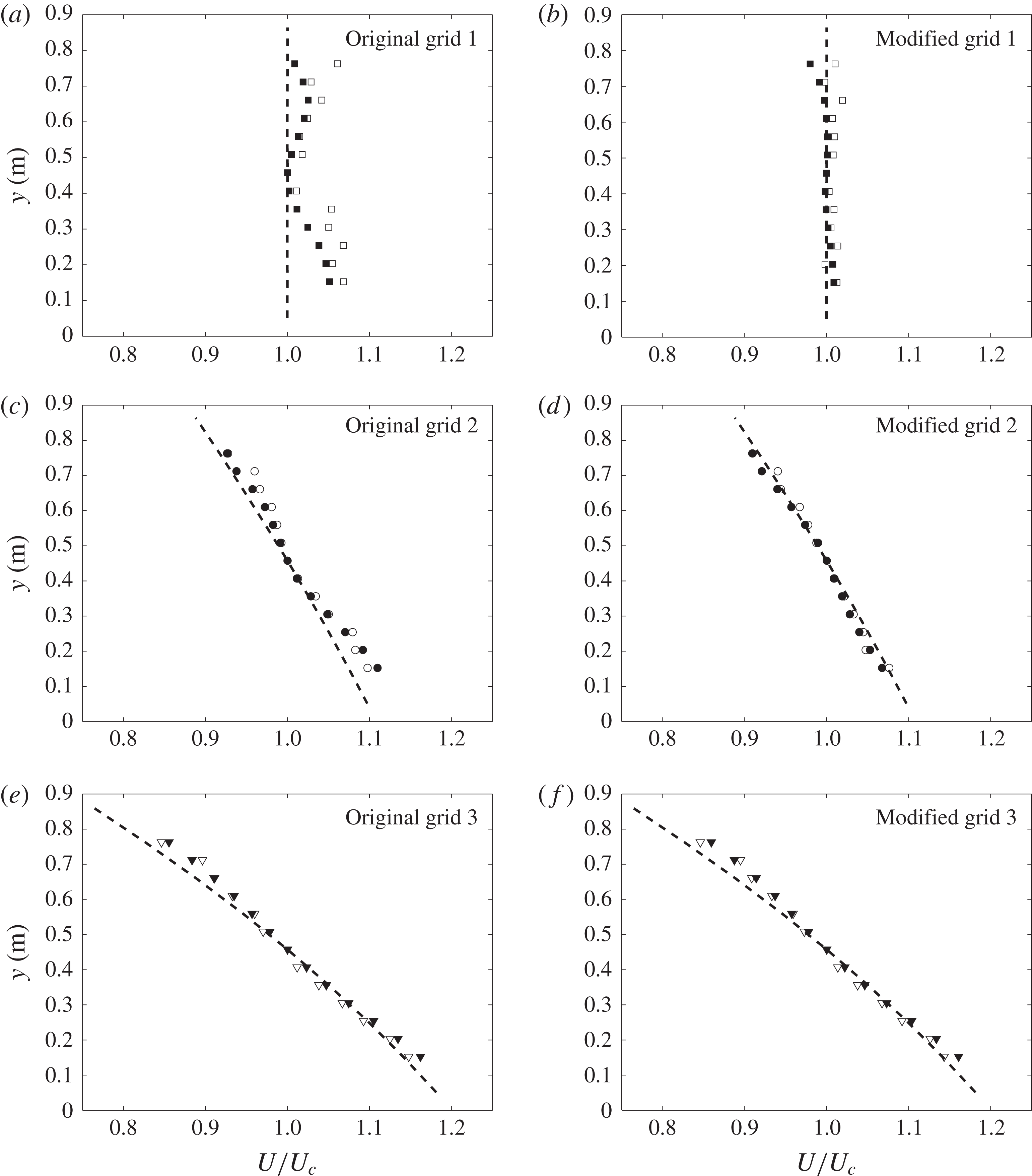
Vertical profiles of the normalized streamwise velocity
 $U/U_{c}$
(symbols) and equation (3.1) (dashed lines) for original grids (with uniform thickness
 $D=10~\text{mm}$
) and modified grids (with variable thickness but uniform aspect ratio). Empty symbols,
 $x=0.83~\text{m}$
; filled symbols,
 $x=4.13~\text{m}$
.

In figure 6(a), we present the vertical profiles of streamwise velocity
 $U$
measured at
 $x=0.83~\text{m}$
and
 $x=4.13~\text{m}$
for the original grids (i.e. with non-uniform
 $C_{D}$
as shown in figure 3
a), together with the profiles calculated using (3.1)–(3.3) with
 $r=0.7$
. Measurements were taken from the middle of the second layer up to the middle of the seventh layer. Note that there was no trial and error involved in generating the velocity profiles. The normalized profiles
 $U/U_{c}$
are presented because the measured incoming velocity (at the beginning of the test section) is different from
 $U_{-0}$
in (3.1) by a constant factor.
A wave-like deviation of the mean velocity profiles across these original grids is observed, especially for grid 1 where the variation of
 $C_{D}$
is the largest. The non-uniform drag coefficient
 $C_{D}$
of the vertical bars in the grid at each layer effectively modifies the local blockage ratio and consequently the local mean velocity. Other than that, the shapes of the velocity profiles generally follow the model, and the shape of the mean profiles is maintained within the measurement range of approximately
 $x/H=1{-}4.5$
. This is consistent with previous conclusions from the parallel wire-generated or plate-generated shear flows (e.g. Rose Reference Rose1966; Champagne et al.
Reference Champagne, Harris and Corrsin1970; Shen & Warhaft Reference Shen and Warhaft2000).
The measurements behind the modified grids, as described in § 2.2, are given in figure 6(b). It is obvious that both grids 1 and 2 collapse better with the predicted profile when the non-uniformity of
 $C_{D}$
is eliminated. This shows that the drag coefficient indeed affects the mean velocity profile quite significantly. As for grid 3, the only modified layer is the bottom one, which is outside the measurement range, and thus the mean velocity profiles of the original and modified grids are almost identical. Again, these results are obtained without trial and error, suggesting that (3.1)–(3.3) can serve as a guideline for bespoke design of desired mean velocity profiles using our proposed inhomogeneous multiscale geometries.
For the modified grids, the shape of the mean profiles is also maintained, in fact better than that for the original grids. The absolute values of the averaged mean shear rate
 $|\overline{\unicode[STIX]{x2202}U/\unicode[STIX]{x2202}y}|$
are
 $0.29~\text{s}^{-1}$
,
 $2.97~\text{s}^{-1}$
and
 $4.99~\text{s}^{-1}$
for grids 1, 2 and 3, respectively. These shear rates are rather small compared to those of Champagne et al. (Reference Champagne, Harris and Corrsin1970) and Harris et al. (Reference Harris, Graham and Corrsin1977). Nevertheless, higher shear rates could in theory be achieved by increasing the gradient of blockage ratio
 $\unicode[STIX]{x1D70E}_{n}$
of the grid, as long as
 $\unicode[STIX]{x1D70E}_{max}$
does not exceed the limit required to avoid recirculations, e.g.
 $\unicode[STIX]{x1D70E}_{max}=35\,\%$
for the current case.
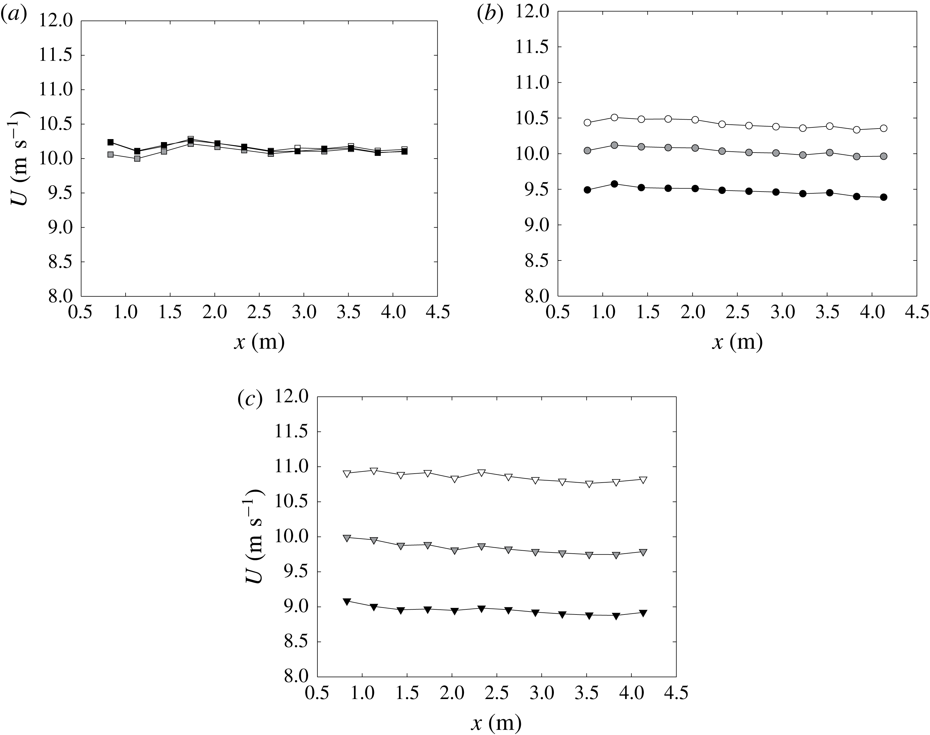
Figure 7 shows the mean velocity profiles along the streamwise direction downstream of the modified grids measured at
 $y=0.25~\text{m}$
,
 $y=0.46~\text{m}$
and
 $y=0.66~\text{m}$
with streamwise step of
 $\unicode[STIX]{x0394}x=0.3~\text{m}$
. The difference between the profiles at each
 $y$
position indicates the shear rate of the flow. The linear fit of the centreline profiles along
 $x$
gives slopes of
 $0.0092$
,
 $-0.043$
, and
 $-0.067$
, respectively, and it is concluded that the mean velocity is roughly constant along the streamwise direction. This also coincides with the velocity profiles observed in figure 6. In the rest of the paper, only modified grids are discussed to exclude the unwanted velocity variations caused by the non-uniform
 $C_{D}$
of the original grids.
Streamwise velocity profiles for modified (a) grid 1, (b) grid 2 and (c) grid 3, at
 $y=0.25~\text{m}$
(white),
 $y=0.46~\text{m}$
(grey) and
 $y=0.66~\text{m}$
(black).

3.2 Turbulence intensities
Profiles of turbulence intensity
 $u^{\prime }/U_{\infty }$
(empty symbols),
 $v^{\prime }/U_{\infty }$
(filled symbols) along (a) streamwise direction
 $x$
at the centreline
 $y=0.46~\text{m}$
, and (b) vertical direction at
 $x=0.83~\text{m}$
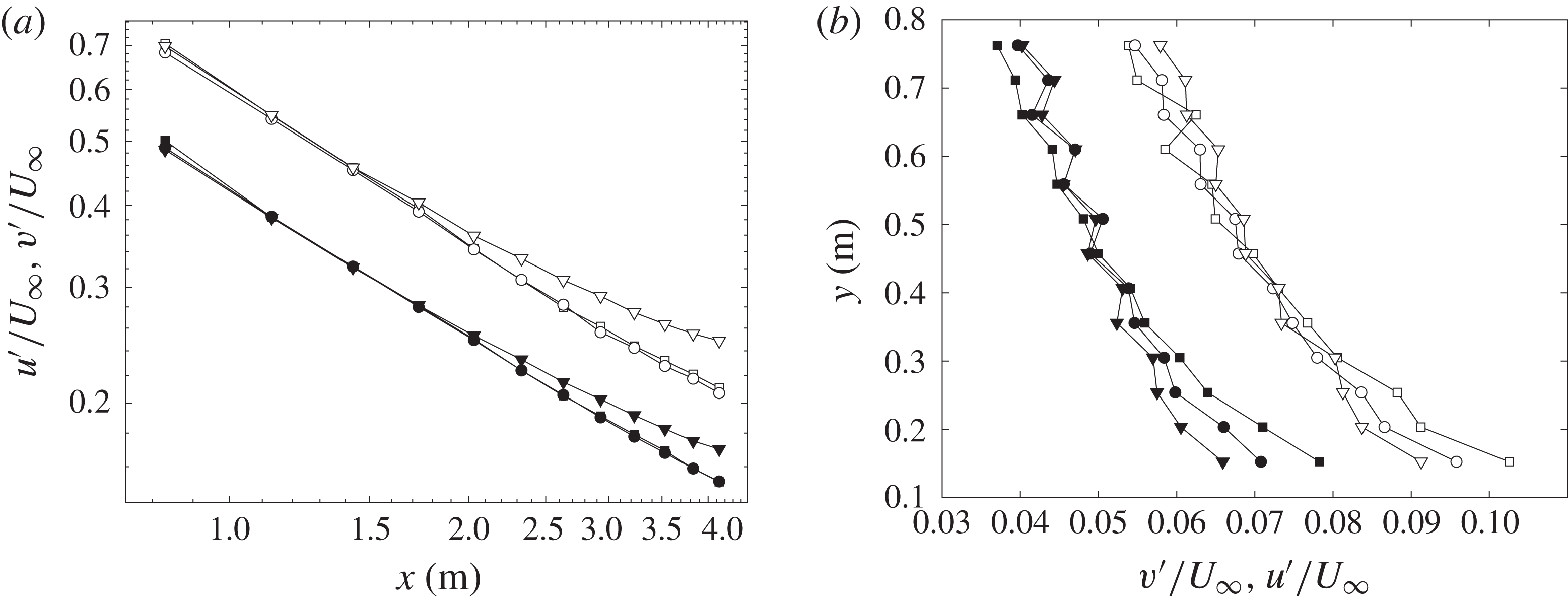
for grid 1 (square), grid 2 (circle) and grid 3 (triangle).

To begin this section, we present the turbulence intensities measured at different streamwise locations. The profiles of
 $u^{\prime }/U_{\infty }$
and
 $v^{\prime }/U_{\infty }$
are plotted along the centreline at
 $y=0.46~\text{m}$
in figure 8(a). The decay of both
 $u^{\prime }$
and
 $v^{\prime }$
is obvious, and the value of
 $v^{\prime }$
is always smaller than
 $u^{\prime }$
for each individual grid at all locations, and approximately follows
 $u^{\prime 2}=2v^{\prime 2}$
, which is consistent with many previous observations in various turbulent shear flows (e.g. Champagne et al.
Reference Champagne, Harris and Corrsin1970; Tavoularis & Corrsin Reference Tavoularis and Corrsin1981; Garg & Warhaft Reference Garg and Warhaft1998; Vanderwel & Tavoularis Reference Vanderwel and Tavoularis2014). The averaged ratio of
 $u^{\prime 2}/v^{\prime 2}$
throughout all
 $x$
locations along the centreline for grid 1, 2, 3 is 1.93, 1.90, 2.07, respectively. The value of
 $u^{\prime }/U_{\infty }$
for all grids at different
 $y$
locations drops from approximately
 $7$
to 2 % along the streamwise direction, and it seems for grid 3 that the streamwise turbulence level
 $u^{\prime }$
remains higher than the others. This might be explained by the higher drag coefficient
 $C_{D}$
as shown in figure 3, and the larger mean shear rate of grid 3, which generates turbulence intensity through production and keeps the turbulence level higher than the other grids.
In figure 8(b), we plot
 $u^{\prime }/U_{\infty }$
and
 $v^{\prime }/U_{\infty }$
along the shear direction
 $y$
at
 $x=0.83~\text{m}$
. Both components of the turbulence profiles show a gradient along the shear direction, and the largest value of
 $u^{\prime }/U_{\infty }$
reaches above
 $10\,\%$
even at
 $x=0.83~\text{m}$
(or
 $x/H=0.9$
). This is quite large compared to conventional grid-generated turbulence, where the turbulence decays rapidly downstream of the grid, and it suggests that it is possible to increase the turbulence level using the vertical bars. This can be of practical importance for experiments that require large turbulence intensities at a distance downstream of the grid. From this point of view, it is desired to have a quantitative scaling relation for
 $u^{\prime }(x,y)$
.
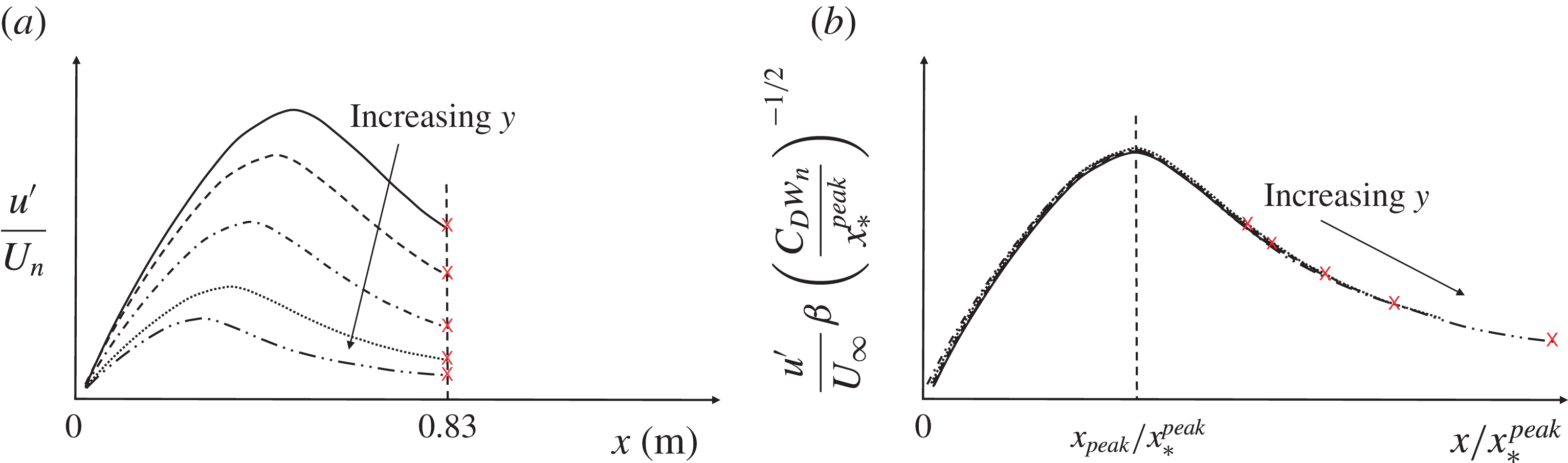
Schematic sketch to show the scaling method of the normalized turbulence intensities along
 $y$
. Different line types represent the streamwise turbulence intensity developments behind different layers of the grid.

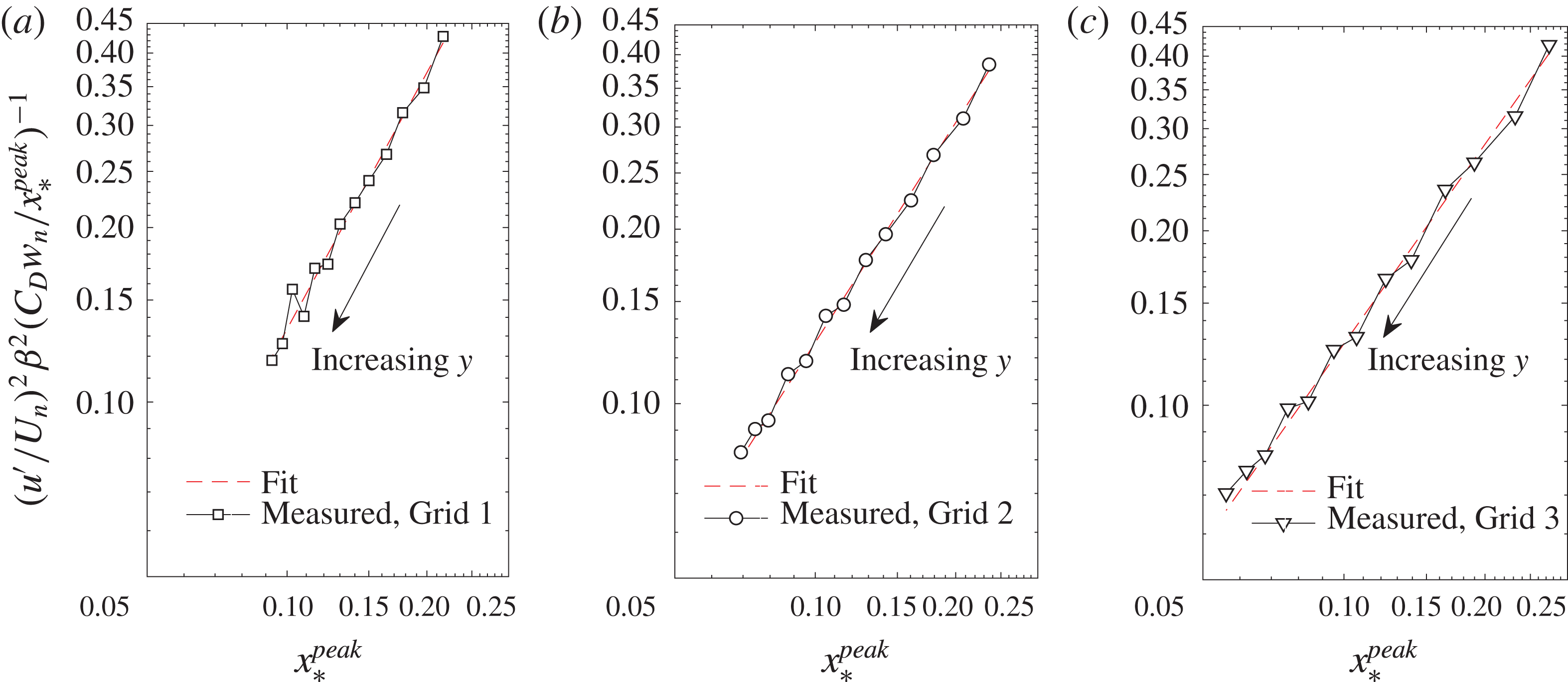
Scaling of the normalized turbulence intensity profiles
 $u^{\prime }(y)$
measured at
 $x=0.83~\text{m}$
for (a) grid 1, (b) grid 2, (c) grid 3, respectively.

To scale the turbulence intensity profiles
 $u^{\prime }(y)$
at given
 $x$
closely downstream of the grid, we refer to the work of Gomes-Fernandes et al. (Reference Gomes-Fernandes, Ganapathisubramani and Vassilicos2012) mentioned in the introduction. The streamwise turbulence intensity level therefore depends on the streamwise development of the turbulence behind each layer of the grid, as shown in figure 9(a), where the turbulence level and peak location varies from layer to layer. This peak location
 $x_{peak}$
is different for different layers but scales with the wake interaction length scale
 $x_{\ast }^{peak}$
, which is itself different at different layers
 $n$
. The results of Gomes-Fernandes et al. (Reference Gomes-Fernandes, Ganapathisubramani and Vassilicos2012) also suggest that the turbulence intensity at the peak location can be collapsed in the form
 $(u^{\prime }/U_{n})\unicode[STIX]{x1D6FD}(C_{D}w_{n}/x_{\ast ,n}^{peak})^{-1/2}$
, where
 $\unicode[STIX]{x1D6FD}=2.88$
is a constant corresponding to the wake development with laminar incoming flow condition, and
 $U_{n}$
is the mean velocity at layer
 $n$
. Figure 9(b) shows how the streamwise turbulence intensities
 $u^{\prime }(x,y)/U_{n}$
can be collapsed.
The current grids are designed such that the
 $x_{\ast }^{peak}$
at all levels
 $n$
are smaller than the first measurement location
 $x=0.83~\text{m}$
(see figure 4
b), and all the data are therefore in the decay region
 $x/x_{\ast }^{peak}>1$
. We now attempt to use the scalings given in figure 9(b) to establish the
 $y$
-profile of
 $u^{\prime }$
at
 $x=0.83~\text{m}$
.
For a streamwise location
 $x=x_{m}$
,
 $(u^{\prime }/U_{n})\unicode[STIX]{x1D6FD}(C_{D}w_{n}/x_{\ast ,n}^{peak})^{-1/2}$
is a function of
 $x_{m}/x_{\ast ,n}^{peak}$
, where
 $x_{\ast ,n}^{peak}$
varies along the
 $y$
direction, as shown in figure 4. If we assume this function to be a power law, i.e.
 $(u^{\prime }/U_{n})^{2}\unicode[STIX]{x1D6FD}^{2}(C_{D}w_{n}/x_{\ast ,n}^{peak})^{-1}\sim (x_{m}/x_{\ast ,n}^{peak})^{b}$
, and fit our measurements of
 $u^{\prime }(y)/U_{n}$
obtained at
 $x_{m}=0.83~\text{m}$
, we have
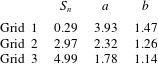
 $b=1.47$
,
 $1.26$
and
 $1.14$
for grids 1, 2 and 3, respectively. It can be observed in figure 10 that the fitted power law functions (dotted line) matches our measurements quite well, which quantitatively relates the downstream turbulence intensities with the geometry of the grid bars, i.e.
 $C_{D}$
,
 $w_{n}$
and
 $g_{n}$
.
3.3 A general grid design approach
Based on the mean velocity model from § 3.1, and the turbulence intensity scaling from § 3.2. We now outline a possible procedure to design a grid to produce a flow with bespoke mean velocity and turbulence profiles.
First, the desired mean velocity profile
 $U_{target,n}$
is used as an input for (3.1)–(3.3) to solve for the blockage ratio
 $\unicode[STIX]{x1D70E}_{n}$
, subject to
 $\unicode[STIX]{x1D70E}_{n}<0.4$
to prevent recirculation. The average blockage ratio
 $\overline{\unicode[STIX]{x1D70E}_{n}}$
can be set to limit the pressure drop, which is
 $\overline{\unicode[STIX]{x1D70E}_{n}}=0.25$
in this case. The problem can be solved by minimizing the error
 $E_{1}$
between the calculated value of
 $U_{n}$
and the desired value
 $U_{target,n}$
, which can be defined as
 $E_{1}=\sum [U_{n}(\unicode[STIX]{x1D70E}_{n})-U_{target,n}]^{2}$
. Therefore the problem becomes to find
 $$\begin{eqnarray}\displaystyle \left.\begin{array}{@{}c@{}}\min E_{1}(\unicode[STIX]{x1D70E}_{n}),\\ s.t.\unicode[STIX]{x1D70E}_{n}<0.4,\overline{\unicode[STIX]{x1D70E}_{n}}=0.25.\end{array}\right\} & & \displaystyle\end{eqnarray}$$
For a uniform shear flow across the test section, the maximum mean shear rate one can achieve using this method depends on the physical size of the wind tunnel because the maximum blockage ratio is always limited by
 $\unicode[STIX]{x1D70E}\leqslant 0.4$
, and the maximum variation of blockage ratio is
 $(\unicode[STIX]{x0394}\unicode[STIX]{x1D70E})_{max}=0.4$
, which constrains the maximum variation of the mean velocity
 $\unicode[STIX]{x0394}U$
. The mean shear rate
 $\text{d}U/\text{d}y$
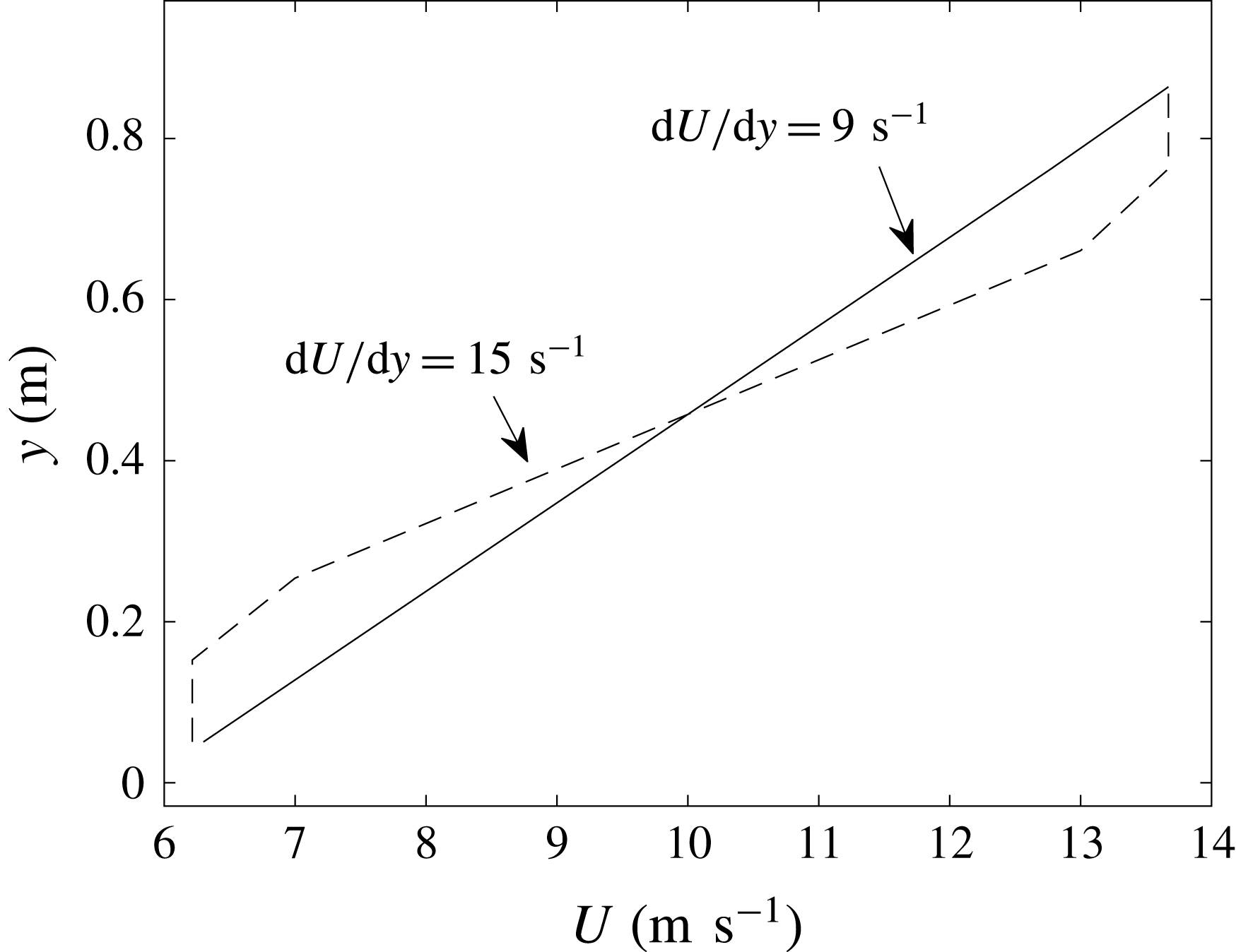
will therefore become larger for a smaller physical domain. For example, for a uniform shear flow, the maximum mean shear rate could be achieved in the current facility (with test section of height
 $H=0.91~\text{m}$
) is approximately
 $9~\text{s}^{-1}$
, but higher mean shear rates could be achieved if only part of the test section is of interest, as demonstrated in figure 11.
Calculated mean velocity profile to demonstrate the maximum mean shear rates achievable in a wind tunnel test section for the case of a uniform shear flow (solid line), and the case where only part of the test section is of interest (dashed line).

Secondly, as shown in the previous section, at a streamwise location
 $x=x_{m}$
, such that
 $x_{m}/x_{\ast }^{peak}>1$
, we have the scaling relation for the turbulence intensity profile along the
 $y$
direction
 $u^{\prime }(y)$
that
 $(u^{\prime }/U_{n})^{2}\unicode[STIX]{x1D6FD}^{2}(C_{D}w_{n}/x_{\ast ,n}^{peak})^{-1}=a(x_{m}/x_{\ast ,n}^{peak})^{b}$
, where
 $\unicode[STIX]{x1D6FD}=2.88$
, and
 $C_{D}=2.9$
for the current study. The turbulence intensity along the
 $y$
direction can be therefore expressed as
 $u^{\prime }/U_{n}=f_{1}(\unicode[STIX]{x1D6FD},C_{D},w_{n},x_{m},x_{\ast ,n}^{peak},a,b)$
, where
 $w_{n}$
is the width of the vertical bars at layer
 $n$
,
 $a$
and
 $b$
are constants and
 $x_{\ast ,n}^{peak}$
is the interaction length scale at layer
 $n$
. The width of the grid bar
 $w_{n}$
is determined by
 $w_{n}=f_{2}(\unicode[STIX]{x1D70E}_{n},c_{n},\ast )$
(where
 $c_{n}$
is the number of the grid bars at layer
 $n$
, and
 $\ast$
stands for other geometry details of the grid such as the overall width
 $W$
and thickness of the horizontal bars, see (2.1)). Since the gap between adjacent vertical bars is defined by
 $g_{n}=W/c_{n}$
, the interaction length scale
 $x_{\ast ,n}^{peak}=0.21g_{n}^{2}/(\unicode[STIX]{x1D6FC}C_{D}w_{n})$
(
 $\unicode[STIX]{x1D6FC}$
is a constant characterizing the incoming flow condition) can be written as
 $x_{\ast ,n}^{peak}=f_{3}(c_{n},C_{D},\ast )$
. Finally, we have
 $u^{\prime }=f(U_{n},\unicode[STIX]{x1D6FD},C_{D},\unicode[STIX]{x1D70E}_{n},c_{n},x_{m},a,b,\ast )$
with only three unknown variables, i.e.
 $c_{n}$
,
 $a$
and
 $b$
. Given a target shape of the turbulence root-mean-square (r.m.s.) velocity profile
 $u_{target,n}^{\prime }$
, the solution of the problem might be solved by minimizing the error
 $E_{2}=\sum [u^{\prime }-u_{target,n}^{\prime }]^{2}$
. Note that the values of
 $a$
and
 $b$
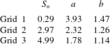
cannot be determined analytically based on the current measurements, but their values seem to vary as a function of the mean shear rate
 $S_{n}$
for a profile
 $u^{\prime }(y)$
measured at a given streamwise location
 $x_{m}$
, as shown in table 2. This table gives a possible range of the values of
 $a$
and
 $b$
, which might be used as a reference to set up the optimization problem. The problem becomes the minimization of
 $$\begin{eqnarray}\displaystyle \left.\begin{array}{@{}c@{}}\min E_{2}(c_{n},a,b,\ast ),\\ s.t.\;a\in {\mathcal{R}},b\in {\mathcal{R}},a=f_{a}(S_{n}),b=f_{b}(S_{n}),\\ c_{n}\in {\mathcal{Z}},c_{n}\in [lb,ub],\end{array}\right\} & & \displaystyle\end{eqnarray}$$
where
 $a$
and
 $b$
are expressed as functions of the mean shear rate. The solution of the problem fully determines the geometry of the grid, and the shape of the target turbulence r.m.s. velocity profile
 $u^{\prime }(y)$
could be achieved at a streamwise location
 $x_{m}/x_{\ast }^{peak}>1$
. The exact value of the turbulence intensity may not be achieved perfectly as yet, because
 $a$
and
 $b$
cannot be prescribed explicitly based on the current results. However, this procedure does ensure that the shape of the target profile is produced downstream of
 $x_{\ast ,n}^{peak}$
. The lower bound
 $lb$
of
 $c_{n}$
, is set to
 $2$
, which ensures that each layer has at least two vertical bars. The upper bound
 $ub$
of
 $c_{n}$
is determined using (2.1) and varies between set-ups. For example, assuming a 10 mm streamwise thickness of the grid, the minimum width of the vertical bar is
 $w_{min}=0.017$
given an aspect ratio
 $AR=0.6$
, which then determines the maximum possible
 $c_{n}$
for each layer.
Variation of the fitting constants
 $a$
and
 $b$
at different mean shear rates, fitted using measurements at
 $x=0.83~\text{m}$
along the
 $y$
direction.
Since the number of bars
 $c_{n}$
is restricted to be integers, the problem is solved by mixed integer nonlinear programming (MINLP), which is an active subject of research in optimization. There are many solvers available, and the results can be compared between different algorithms to give confidence. In principle, a homogeneous shear seems possible using this method where a linear profile of
 $U_{target,n}$
and a constant
 $u_{target,n}^{\prime }$
are used as input to each one of these steps. This approach gives the framework of the grid design method, and the constraints in the problem can be improved and broadened to a wider range of turbulent shear flows with further studies.
3.4 Reynolds shear stress
In preparation of the model that we develop in § 3.5 to describe the streamwise evolution of the profiles
 $u^{\prime }(y)$
from
 $x=0.83~\text{m}$
to larger values of
 $x$
, we study in this section the streamwise development of the shear correlation coefficient
 $\unicode[STIX]{x1D70C}\equiv -\overline{uv}/u^{\prime }v^{\prime }$
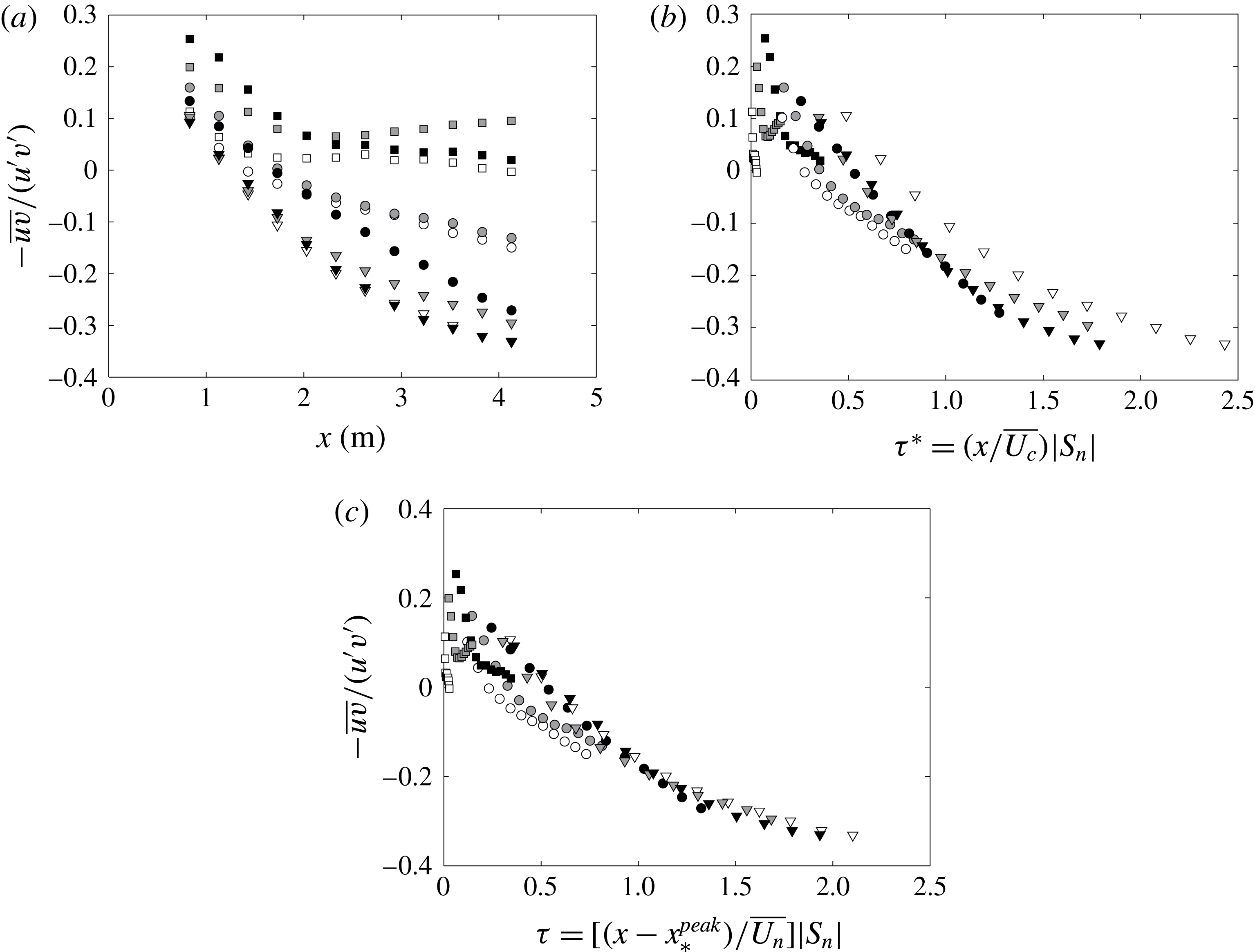
given in figure 12(a). It can be observed that, except for grid 1, all values decrease monotonically with streamwise distance. It is interesting to explore if there is a scaling relation that collapses these data. We first look at the dimensionless time scale
 $\unicode[STIX]{x1D70F}^{\ast }\equiv (x/\overline{U_{c}})|S_{n}|=(x/\overline{U_{c}})|\overline{\unicode[STIX]{x2202}U_{n}/\unicode[STIX]{x2202}y}|$
(where
 $\overline{U_{c}}$
is the streamwise mean velocity averaged over the
 $x$
along the centreline at
 $y=0.46~\text{m}$
) used in previous studies as this is an important parameter to describe the evolution of shear flows. The results are shown in figure 12(b), and
 $\overline{U_{n}}$
and
 $S_{n}\equiv \overline{\unicode[STIX]{x2202}U_{n}/\unicode[STIX]{x2202}y}$
are the averages of values measured at
 $x=0.83~\text{m}$
and
 $x=4.13~\text{m}$
. It is clear that the data do not collapse, especially for grid 2 and 3. If we use a modified local dimensionless time scale defined as
 $\unicode[STIX]{x1D70F}\equiv [(x-x_{\ast ,n}^{peak})/\overline{U_{n}}]|S_{n}|$
, it can be seen that
 $\unicode[STIX]{x1D70C}$
is collapsed fairly well for
 $\unicode[STIX]{x1D70F}\geqslant 0.8$
. This definition of
 $\unicode[STIX]{x1D70F}$
replaces
 $\overline{U_{c}}$
with
 $\overline{U_{n}}$
, and includes the wake interaction length scale
 $x_{\ast ,n}^{peak}$
as the virtual origin, since
 $x_{\ast }^{peak}$
marks the starting location of decay that varies from layer to layer for each grid. This new definition of
 $\unicode[STIX]{x1D70F}$
is equivalent to a translation of
 $\unicode[STIX]{x1D70F}^{\ast }$
for regular grids, where
 $x_{\ast }^{peak}$
is constant at all positions. The results can be compared between figure 12(b,c), where the profiles of
 $\unicode[STIX]{x1D70C}$
of grids 2 and 3 collapse much better with
 $\unicode[STIX]{x1D70F}$
.
Streamwise development of
 $-\overline{uv}/u^{\prime }v^{\prime }$
for grid 1 (square), grid 2 (circle) and grid 3 (triangle) along the streamwise direction at
 $y=0.25~\text{m}$
(white),
 $y=0.46~\text{m}$
(grey) and
 $y=0.66~\text{m}$
(black) versus (a) streamwise location
 $x$
, (b) local dimensionless time scale
 $\unicode[STIX]{x1D70F}^{\ast }\equiv (x/\overline{U_{c}})|S_{n}|$
, and (c) local dimensionless time scale
 $\unicode[STIX]{x1D70F}\equiv [(x-x_{\ast ,n}^{peak})/\overline{U_{n}}]|S_{n}|$
with virtual origin
 $x_{\ast ,n}^{peak}$
.

In several previous experiments (e.g. Rose Reference Rose1966; Harris et al.
Reference Harris, Graham and Corrsin1977; Tavoularis & Corrsin Reference Tavoularis and Corrsin1981; Tavoularis & Karnik Reference Tavoularis and Karnik1989; Nedić & Tavoularis Reference Nedić and Tavoularis2016) it has been shown that the value of the shear correlation coefficient
 $\unicode[STIX]{x1D70C}$
increases downstream along the centreline and eventually reaches a magnitude of approximately 0.45–0.5. For the current results, it is interesting that the shear coefficient
 $\unicode[STIX]{x1D70C}$
changes sign for grids 2 and 3, but not for grid 1. Figure 12(b,c) suggest that the flow is greatly disrupted by the initial conditions that have an effect up to approximately
 $\unicode[STIX]{x1D70F}=0.8$
, downstream of which the Reynolds shear stress starts to play a significant role. This makes sense by looking at grid 1 whose shear coefficient remains positive all the time and close to zero. The range of dimensionless time scale
 $\unicode[STIX]{x1D70F}$
is not large enough to show the asymptote value of
 $\unicode[STIX]{x1D70C}$
(where
 $0.45<|\unicode[STIX]{x1D70C}|<0.5$
), although it seems that the change rate of
 $\unicode[STIX]{x1D70C}$
is decreasing with
 $\unicode[STIX]{x1D70F}$
, which is consistent with previous literature.
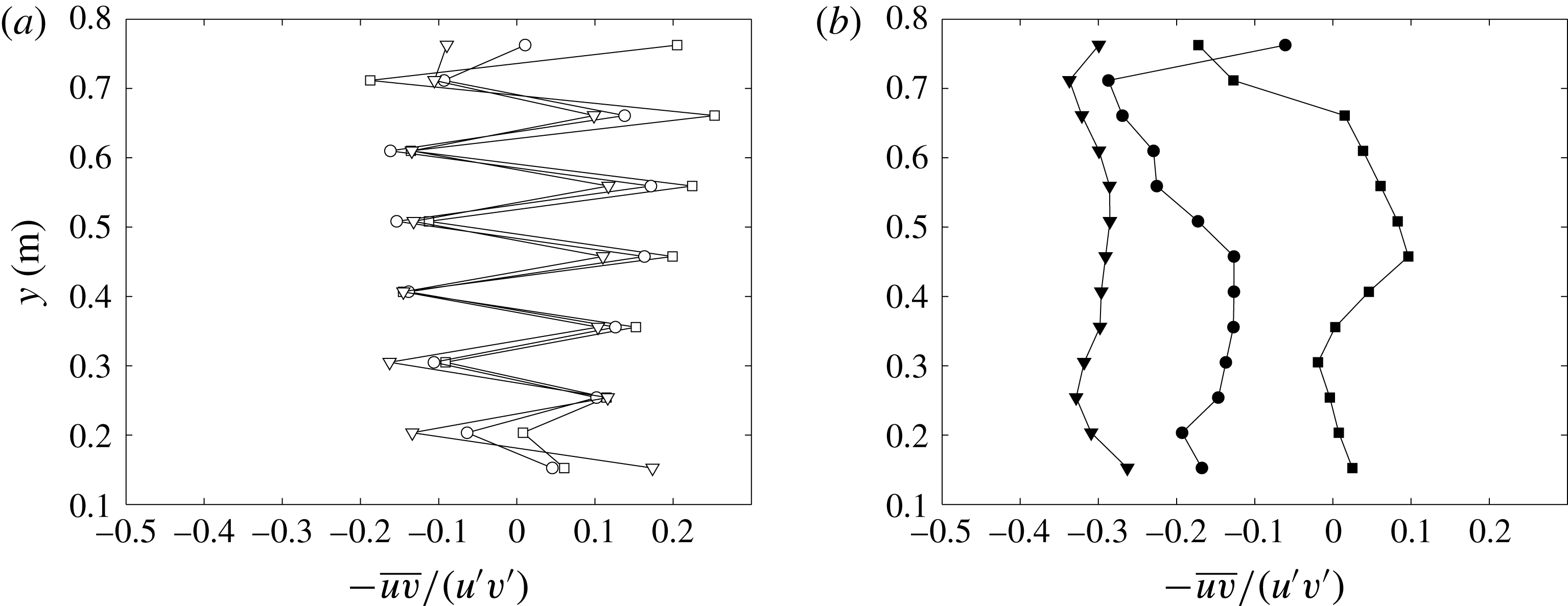
Vertical profiles of
 $-\overline{uv}/u^{\prime }v^{\prime }$
for grid 1 (square), grid 2 (circle) and grid 3 (triangle) at (a)
 $x=0.83~\text{m}$
(empty symbols) and (b)
 $x=4.13~\text{m}$
(filled symbols).

Comparison of shear correlation coefficients measured from independent expriments at
 $x=0.83~\text{m}$
and different
 $y$
locations. The 95 % confidence interval (CI) is calculated as
 $CI=1.96\text{cov}(\unicode[STIX]{x1D70C}_{v},\unicode[STIX]{x1D70C}_{s})/\sqrt{2}$
, where
 $\unicode[STIX]{x1D70C}_{v}$
,
 $\unicode[STIX]{x1D70C}_{s}$
is the shear correlation coefficient measured from the vertical and streamwise profiles, respectively, and
 $\text{cov}(\unicode[STIX]{x1D70C}_{v},\unicode[STIX]{x1D70C}_{s})$
is the covariance of
 $\unicode[STIX]{x1D70C}_{v}$
,
 $\unicode[STIX]{x1D70C}_{s}$
.

The shear correlation coefficients
 $-\overline{uv}/u^{\prime }v^{\prime }$
along the
 $y$
direction at
 $x=0.83~\text{m}$
and
 $x=4.13~\text{m}$
are shown in figure 13. The oscillatory behaviour at
 $x=0.83~\text{m}$
around
 $-\overline{uv}/u^{\prime }v^{\prime }=0$
is most obvious as the probe moves behind the horizontal bars of the grid at every other
 $y$
location. The large fluctuation of shear correlation coefficients with change of signs were also observed in e.g. Rose (Reference Rose1966) in a streamwise location close to the grid (
 $x/H=1.33$
). The positive-valued data points in figure 13(a) are from measurements taken at the centre of each layer (i.e. behind the vertical bars), which correspond to the data at
 $x=0.83~\text{m}$
given in figure 12(a). This also supports the assumption that direct effects of the grid dominate in the region of
 $\unicode[STIX]{x1D70F}<0.8$
as shown in figure 12. Table 3 gives the error of the shear correlation coefficients from two independent experiments to give confidence in the measurement, indicated by the
 $95\,\%$
confidence interval
 $CI=1.96\text{cov}(\unicode[STIX]{x1D70C}_{x},\unicode[STIX]{x1D70C}_{y})/\sqrt{2}$
, where
 $\text{cov}(\unicode[STIX]{x1D70C}_{s}\unicode[STIX]{x1D70C}_{v})$
is the covariance of
 $\unicode[STIX]{x1D70C}_{s}$
,
 $\unicode[STIX]{x1D70C}_{v}$
measured from the streamwise and vertical profiles, respectively. In figure 13(b), it is observed that the magnitude of the shear coefficients increases from grid 1 to grid 3 (with increasing shear rate), and the variation of
 $-\overline{uv}/u^{\prime }v^{\prime }$
along the
 $y$
direction is much reduced comparing to that measured at
 $x=0.83~\text{m}$
. This is consistent with the streamwise profiles discussed above, and previous observations made by Rose (Reference Rose1966), Garg & Warhaft (Reference Garg and Warhaft1998), Nedić & Tavoularis (Reference Nedić and Tavoularis2016).
3.5 A simplified model for turbulent kinetic energy
To look at the evolution of the
 $y$
profiles of
 $u^{\prime }$
along the streamwise direction
 $x$
, we have to consider the turbulence production by the mean shear rate, and we propose a simplified model to describe how
 $u^{\prime }(x,y)$
evolves in the
 $x$
direction downstream of our grids. To begin with, we neglect the pressure, transport and viscous diffusion terms in the turbulent kinetic energy equation. Harris et al. (Reference Harris, Graham and Corrsin1977) estimated the significance of the transport term by showing that the ratio
 $|(\unicode[STIX]{x2202}\overline{u^{3}}/\unicode[STIX]{x2202}x)/(U_{c}\unicode[STIX]{x2202}\overline{u^{2}}/\unicode[STIX]{x2202}x)|$
is smaller than
 $0.03$
in their experiment, and concluded that the transport term can be omitted. In the current study, this ratio decreases rapidly with streamwise distance away from the grid, and the maximum values on the centreline (at
 $x=0.83~\text{m}$
) are
 $0.0105$
,
 $0.0102$
,
 $0.0113$
for grids 1, 2, 3, respectively. We therefore assume that the transport is relatively small compared to the advection term, and that it can be neglected.
With these assumptions, we keep only the production and dissipation terms in the right-hand side of the kinetic energy equation following Harris et al. (Reference Harris, Graham and Corrsin1977) and Tavoularis & Corrsin (Reference Tavoularis and Corrsin1981), i.e.
 $$\begin{eqnarray}\displaystyle U\frac{\unicode[STIX]{x2202}k}{\unicode[STIX]{x2202}x}=P-\unicode[STIX]{x1D716}. & & \displaystyle\end{eqnarray}$$
Then we write
 $P\cong -\overline{uv}S_{n}=\unicode[STIX]{x1D70C}S_{n}u^{\prime }v^{\prime }=\unicode[STIX]{x1D70C}^{\ast }S_{n}u^{\prime 2}$
, where
 $S_{n}\equiv \overline{\unicode[STIX]{x2202}U_{n}/\unicode[STIX]{x2202}y}$
is the local mean shear rate, and
 $\unicode[STIX]{x1D70C}^{\ast }(x)=\unicode[STIX]{x1D70C}(x)/\sqrt{2}$
because
 $v^{\prime }=u^{\prime }/\sqrt{2}$
as discussed in § 3.2. By assuming that the transverse r.m.s. fluctuating velocity
 $w^{\prime }$
equals
 $v^{\prime }$
, i.e.
 $w^{\prime }=v^{\prime }$
, the turbulent kinetic energy can then be written as
 $k=(1/2)(u^{\prime 2}+2v^{\prime 2})=u^{\prime 2}$
. Finally we write the dissipation
 $\unicode[STIX]{x1D716}$
as
 $\unicode[STIX]{x1D716}=C_{\unicode[STIX]{x1D716}}(k^{3/2}/L)=C_{\unicode[STIX]{x1D716}}(u^{\prime 3}/L)$
, where
 $L=L_{uu,x}(x)$
is the longitudinal integral length scale.
Equation (3.6), for a given
 $n$
or
 $y$
(therefore omitted in the equations for simplicity), now becomes
 $$\begin{eqnarray}\displaystyle U\frac{\unicode[STIX]{x2202}u^{\prime 2}}{\unicode[STIX]{x2202}x}=\unicode[STIX]{x1D70C}^{\ast }(x)Su^{\prime 2}-\frac{C_{\unicode[STIX]{x1D716}}(x)}{L(x)}u^{\prime 3}. & & \displaystyle\end{eqnarray}$$
To continue with a quantitative description of
 $u^{\prime }(x,y)$
, we write (3.7) at given
 $n$
as
 $$\begin{eqnarray}\displaystyle \frac{\text{d}k}{\text{d}x}+\unicode[STIX]{x1D709}(x)k=\unicode[STIX]{x1D701}(x)k^{m}, & & \displaystyle\end{eqnarray}$$
where
 $\unicode[STIX]{x1D709}(x)=-\unicode[STIX]{x1D70C}^{\ast }(x)S/U$
,
 $\unicode[STIX]{x1D701}(x)=-C_{\unicode[STIX]{x1D716}}(x)/(UL(x))$
and
 $m=3/2$
.
The solution of (3.8) is given by
 $$\begin{eqnarray}\displaystyle k=\left(\frac{-\displaystyle \frac{1}{2}\displaystyle \int _{x_{p}}^{x}\text{e}^{-1/2\int _{x_{p}}^{x}-\unicode[STIX]{x1D70C}^{\ast }S/U\,\text{d}x}\left(\frac{-C_{\unicode[STIX]{x1D716}}}{UL}\right)\text{d}x+C}{\text{e}^{-1/2\int _{x_{p}}^{x}-\unicode[STIX]{x1D70C}^{\ast }S/U\,\text{d}x}}\right)^{-2}, & & \displaystyle\end{eqnarray}$$
where we write
 $x_{p}\equiv x_{\ast }^{peak}$
for simplicity. To close (3.9), we need the expressions of
 $\unicode[STIX]{x1D70C}^{\ast }(x)$
,
 $L(x)$
,
 $C_{\unicode[STIX]{x1D716}}(x)$
and the integration constant
 $C$
. Since
 $\unicode[STIX]{x1D70C}(\unicode[STIX]{x1D70F})$
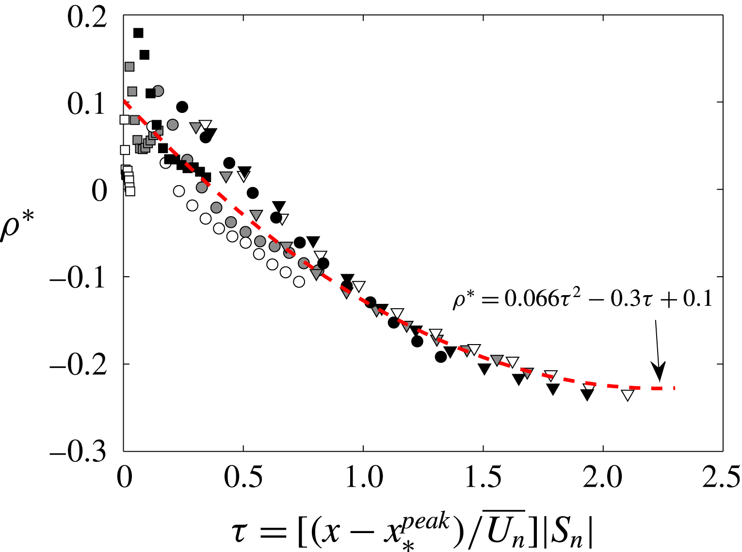
collapses well in the way shown in figure 12(c), we fit
 $\unicode[STIX]{x1D70C}^{\ast }=\unicode[STIX]{x1D70C}/\sqrt{2}$
using a second-order polynomial (dashed lines) as shown in figure 14 to calculate
 $\unicode[STIX]{x1D70C}^{\ast }(x)$
since
 $x_{\ast }^{peak}$
,
 $U_{n}$
and
 $S_{n}$
in
 $\unicode[STIX]{x1D70F}$
are known at given
 $y$
. Here we fit the data with the centreline values of each grid (i.e. grey symbols), and the result captures the evolution of
 $\unicode[STIX]{x1D70C}^{\ast }$
quite well. This fitted function is then used to prescribe
 $\unicode[STIX]{x1D70C}^{\ast }(x)$
given local constants
 $x_{\ast }^{peak}$
,
 $U_{n}$
and
 $S_{n}$
. This fitting method inevitably carries larger error for grid 1 (see figure 14) due to the scatter of
 $\unicode[STIX]{x1D70C}^{\ast }(x)$
at
 $\unicode[STIX]{x1D70F}\approx 0$
. But the mean shear rate produced by grid 1 is approximately 0, and the power
 $(-0.5S/U\int _{x_{p}}^{x}-\unicode[STIX]{x1D70C}^{\ast }\,\text{d}x)$
in the exponential is effectively 0 too, which makes the error for grid 1 insignificant in (3.9).
Streamwise profiles of
 $\unicode[STIX]{x1D70C}^{\ast }$
for grid 1 (square), grid 2 (circle) and grid 3 (triangle) at
 $y=0.25~\text{m}$
(white),
 $y=0.46~\text{m}$
(grey) and
 $y=0.66~\text{m}$
(black) with second-order polynomial fit (dashed lines).

3.5.1 Integral length scale
Longitudinal integral length scale
 $L$
profiles for grid 1 (square), grid 2 (circle) and grid 3 (triangle) at
 $y=0.25~\text{m}$
(white),
 $y=0.46~\text{m}$
(grey) and
 $y=0.66~\text{m}$
(black) versus the streamwise location
 $x$
.

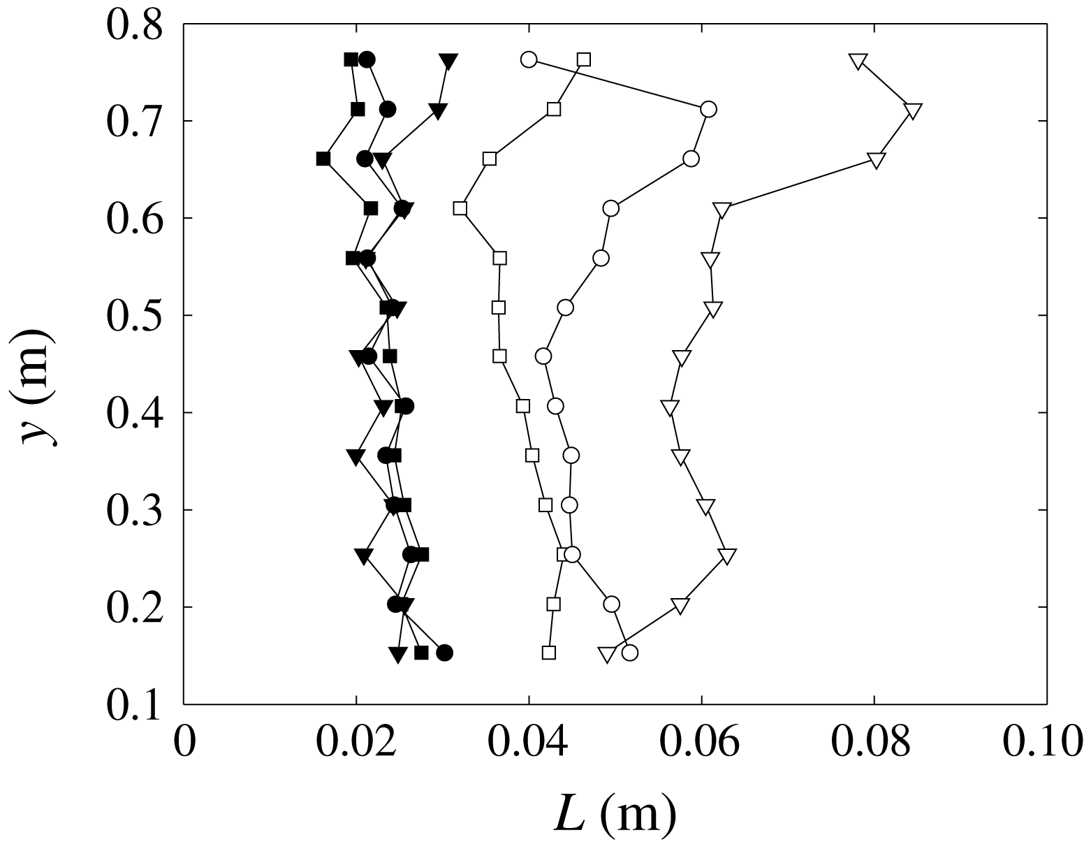
Longitudinal integral length scale
 $L$
profiles for grid 1 (square), grid 2 (circle) and grid 3 (triangle) along the
 $y$
direction at
 $x=0.83~\text{m}$
(filled symbols) and
 $x=4.13~\text{m}$
(empty symbols).

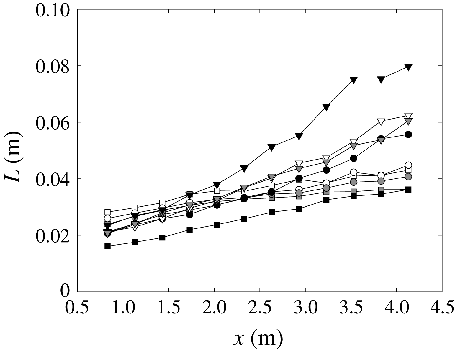
Now we look at the development of the longitudinal integral length scale
 $L$
as a function of the streamwise location
 $x$
for all grids, see figure 15. The length scales are calculated using the corrected spectra as discussed in § 2.3. It is obvious that
 $L$
increases with the streamwise location monotonically. The value of
 $L$
for a given grid at different
 $y$
locations seems to grow linearly at a rate which is practically similar at different
 $y$
locations. This also implies that
 $L$
increases approximately linearly against the local dimensionless time scale
 $\unicode[STIX]{x1D70F}$
as well, which is consistent with Champagne et al. (Reference Champagne, Harris and Corrsin1970) and Harris et al. (Reference Harris, Graham and Corrsin1977).
By looking at the profiles along
 $y$
in figure 16, it seems that
 $L$
remains roughly constant at
 $x=0.83~\text{m}$
. At
 $x=4.13~\text{m}$
, the value of
 $L$
increases from grid 1 (square) to grid 3 (triangle). This makes sense if
 $L\propto \unicode[STIX]{x1D70F}$
, as
 $\unicode[STIX]{x1D70F}$
increases with the mean shear rate
 $S$
at given
 $x$
and
 $U$
.
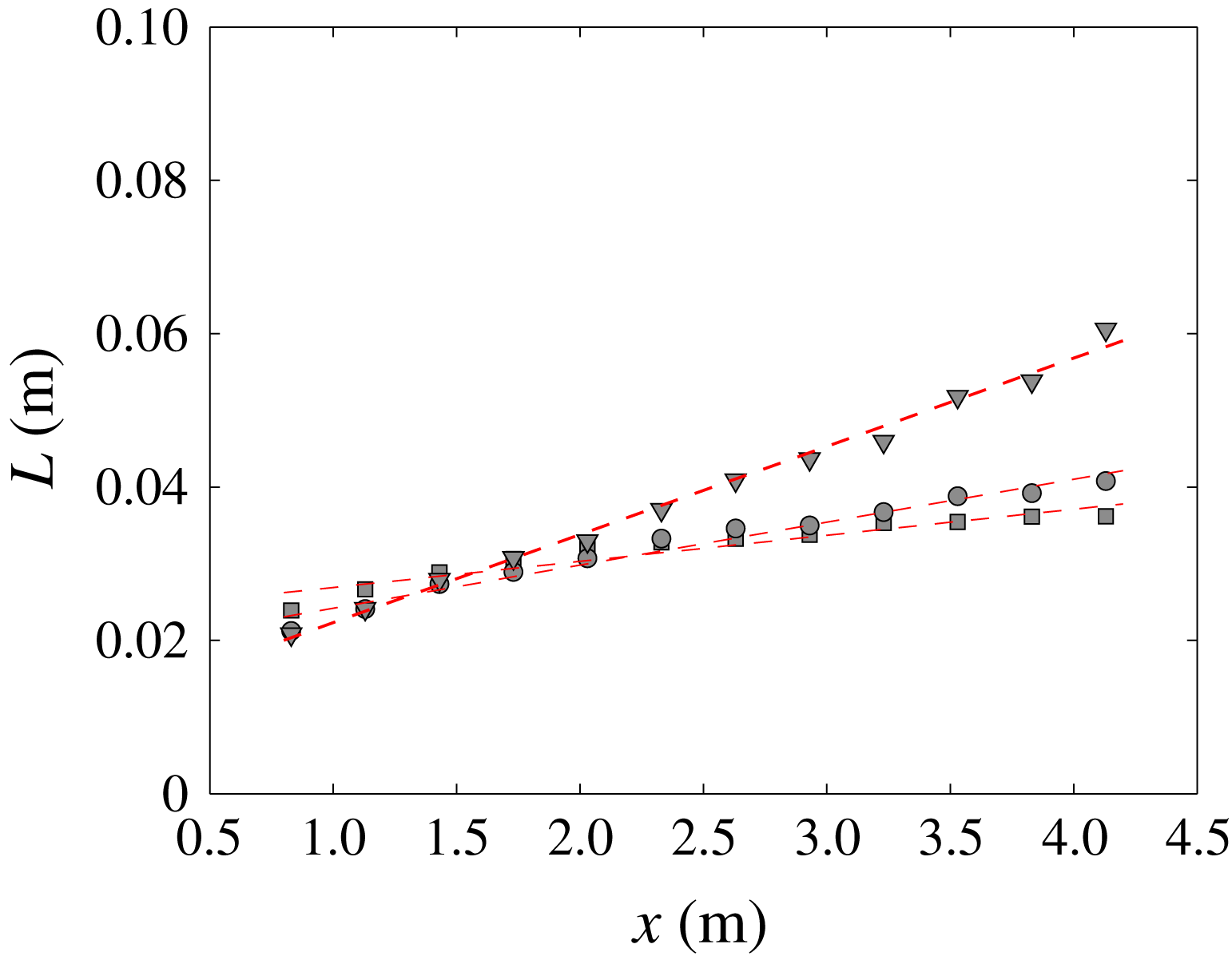
Profiles of longitudinal integral length scale
 $L$
for grid 1 (square), grid 2 (circle) and grid 3 (triangle) along the centreline with linear fitted results (dashed lines).

From figures 15 and 16, we notice that the values of
 $L$
at
 $y=0.66~\text{m}$
are smaller for grid 1 and larger for grid 3, yet the values calculated at this location from the two independent measurements are the same (as shown in figures 15 and 16), which rules out the possibility of measurement/calculation error. The reason for this larger value is not completely clear, but might have to do with the different inlet grid conditions and the related different mean shear rates.
For the purpose of the current discussion, we ignore this outlier, and assume that the rate of increase of
 $L$
for a given grid is independent of
 $y$
. We therefore estimate the streamwise evolution of
 $L$
based on its centreline profile only. The fitted results are given in figure 17, where all three profiles show a linear increase with streamwise distance
 $x$
away from the grid. This is also consistent with previous works such as Champagne et al. (Reference Champagne, Harris and Corrsin1970) and Harris et al. (Reference Harris, Graham and Corrsin1977). We write
 $L(x)=px+q$
, where
 $p$
,
 $q$
are fitting coefficients. The fitted constants are
 $p=0.0034$
, 0.0056, 0.012 and
 $q=0.024$
, 0.019, 0.011 for grid 1, 2, 3, respectively.
3.5.2 Dissipation coefficient
 $C_{\unicode[STIX]{x1D716}}$

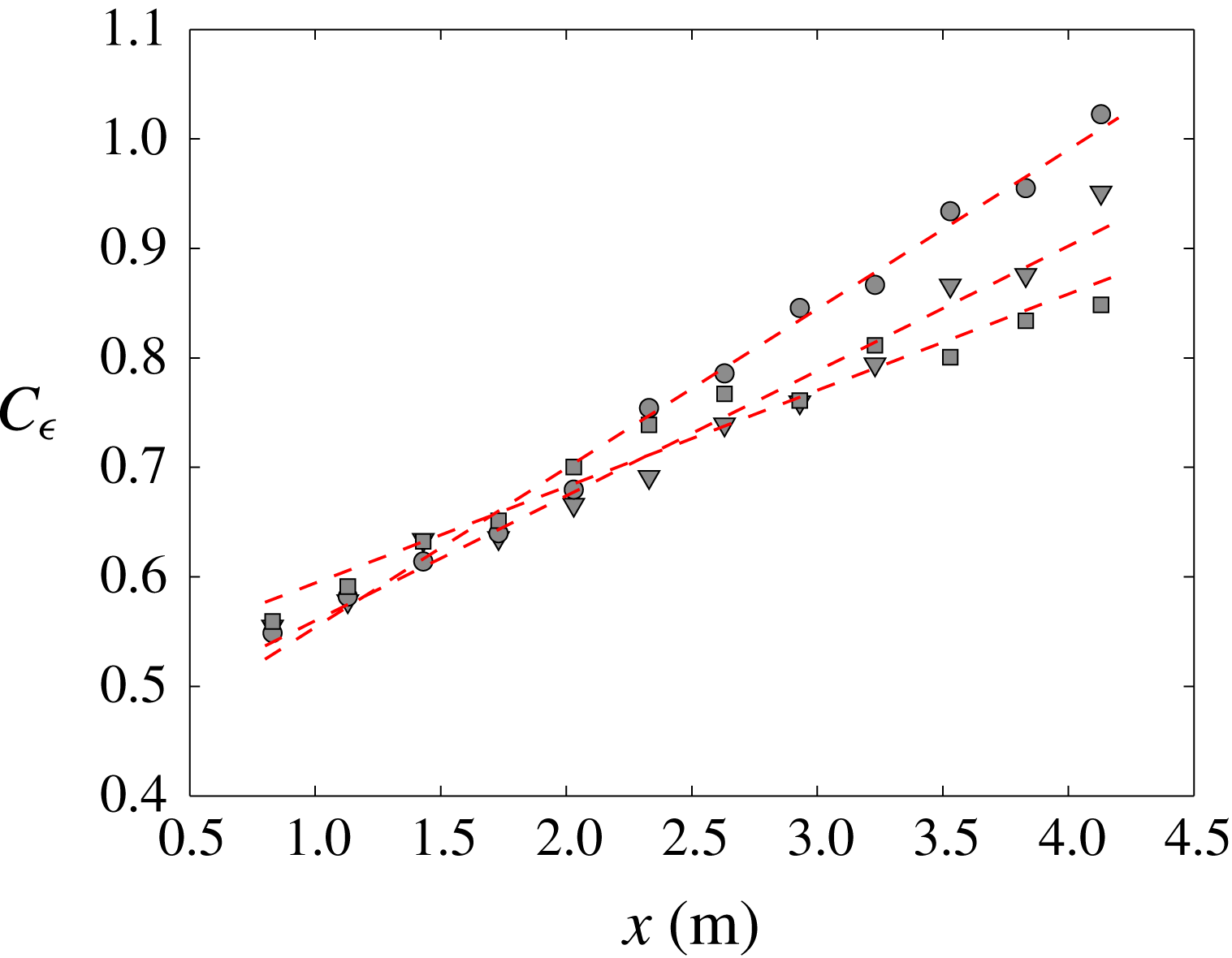
Profiles of
 $C_{\unicode[STIX]{x1D716}}=\unicode[STIX]{x1D716}L/u^{\prime 3}$
for grid 1 (square), grid 2 (circle) and grid 3 (triangle) along the centreline with linear fitted results (dashed lines).

The behaviour of
 $C_{\unicode[STIX]{x1D716}}$
in turbulent shear flow with uniform mean shear rate has been studied by Nedić & Tavoularis (Reference Nedić and Tavoularis2016), where they showed different stages of development with respect to
 $\unicode[STIX]{x1D70F}$
. In figure 18, we show the streamwise development of
 $C_{\unicode[STIX]{x1D716}}=\unicode[STIX]{x1D716}L/u^{\prime 3}$
along the centreline for all three grids. It can be observed that all three profiles increase linearly as
 $C_{\unicode[STIX]{x1D716}}=cx+d$
, where the coefficients
 $c$
,
 $d$
are fitted in a least square sense. The fitted constants are
 $c=0.088$
, 0.15, 0.11 and
 $d=0.51$
, 0.41, 0.45 for grids 1, 2, 3 respectively. This linear increase of
 $C_{\unicode[STIX]{x1D716}}$
with
 $x$
is in agreement with Nedić & Tavoularis (Reference Nedić and Tavoularis2016) in their initial region.
Ratio of
 $\unicode[STIX]{x1D716}$
and modelled term
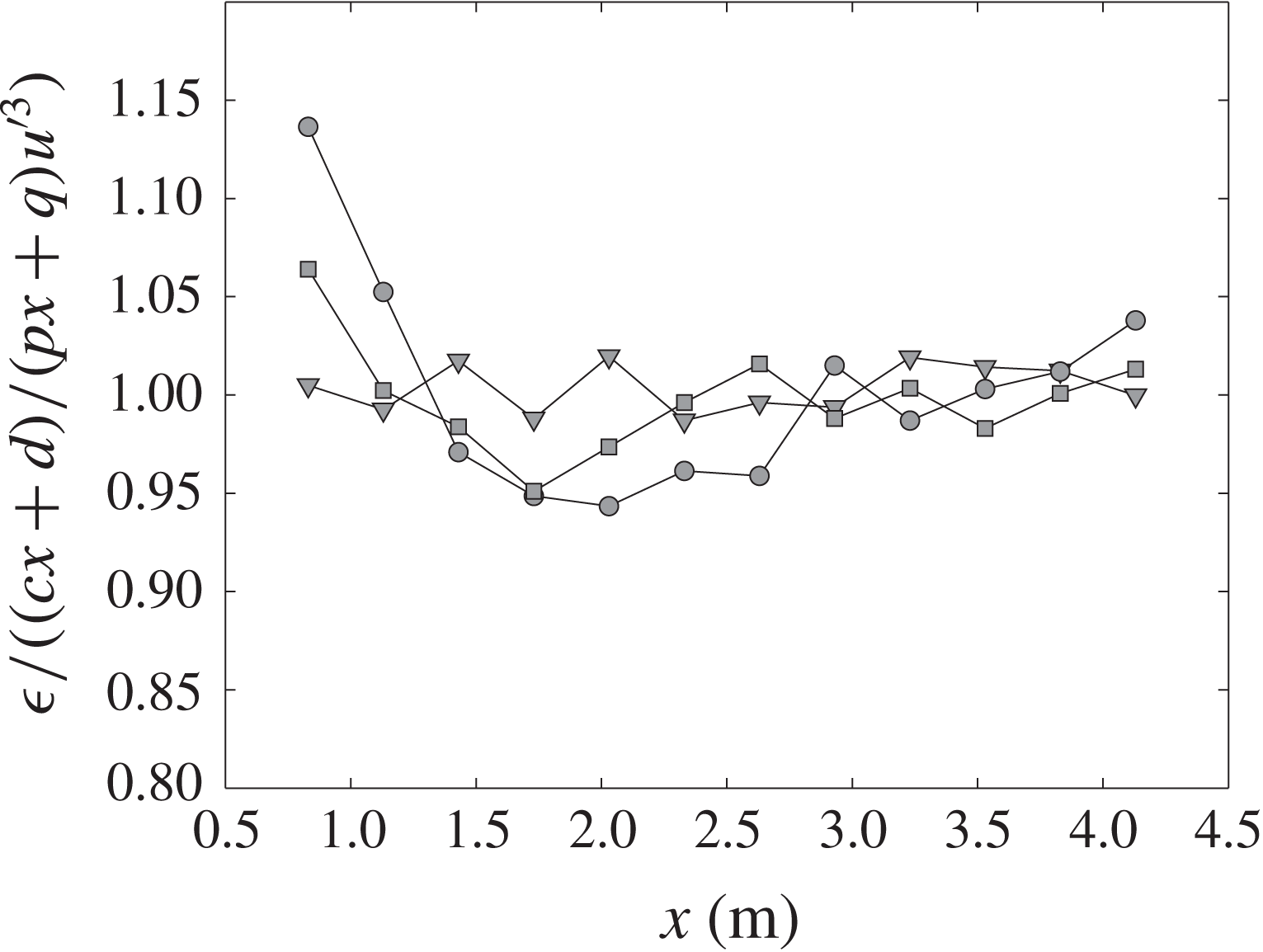
 $(cx+d)/(px+q)u^{\prime 3}$
grid 1 (square), 2 (circle) and 3 (triangle), respectively, along the centreline.

To check the quality of our linear fits of
 $C_{\unicode[STIX]{x1D716}}(x)$
and
 $L(x)$
, we plot the ratio
 $\unicode[STIX]{x1D716}/(C_{\unicode[STIX]{x1D716}}u^{\prime 3}/L)$
as
 $\unicode[STIX]{x1D716}/((cx+d)u^{\prime 3}/(px+q))$
in figure 19. It is observed that this ratio is within
 $\pm 5\,\%$
of unity for all three grids, with the exception of the first point.
3.5.3 Predicting streamwise evolution
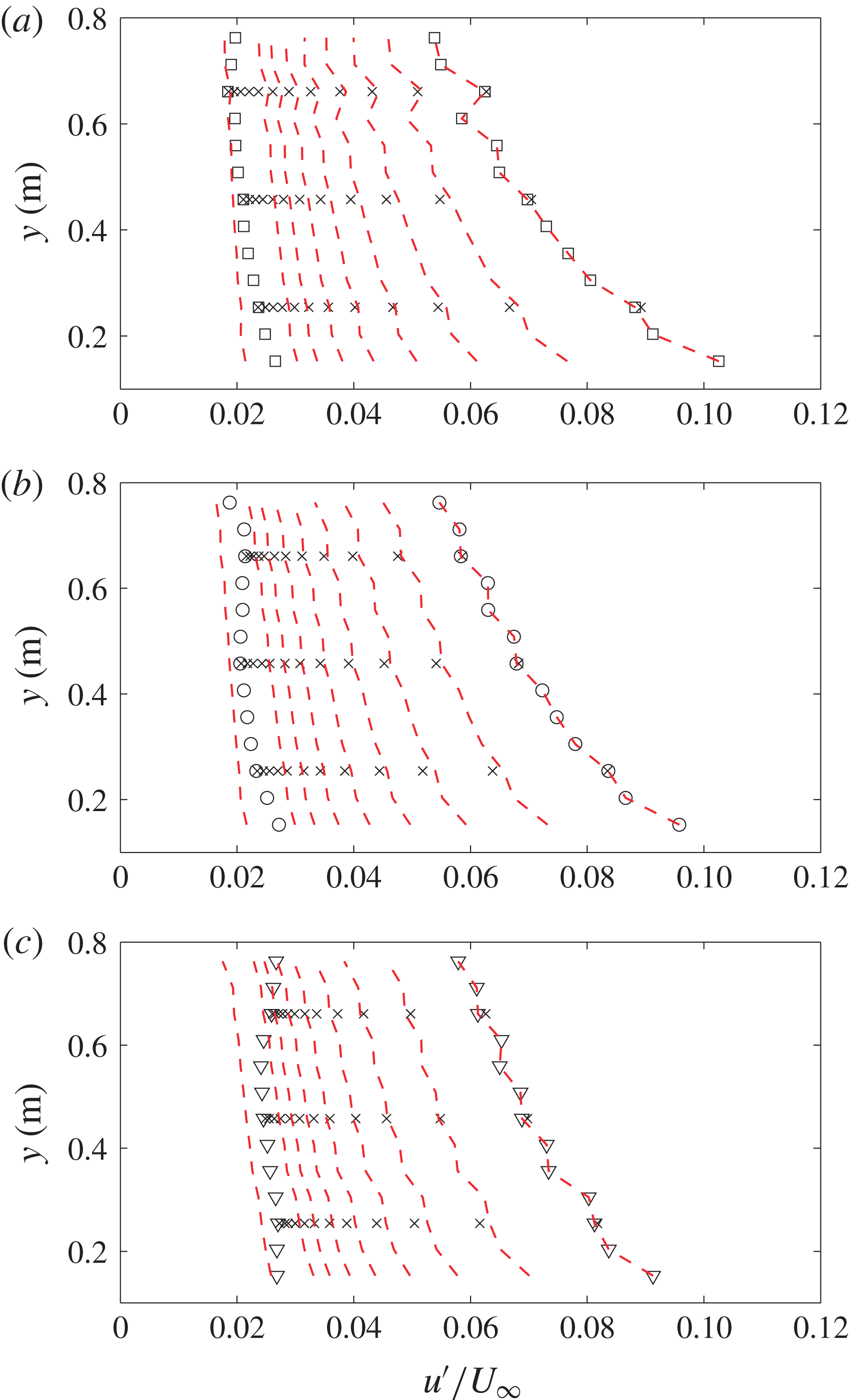
Turbulence intensity profiles
 $u^{\prime }/U_{\infty }$
for (a) grid 1 (square), (b) grid 2 (circle) and (c) grid 3 (triangle). Empty symbols are vertical profiles measured at
 $x=0.83~\text{m}$
and
 $x=4.13~\text{m}$
. Cross symbols are streamwise profiles measured at given
 $y$
location. Dashed red lines are predictions calculated using the vertical profile and centreline profile.

With the fitted functions of
 $\unicode[STIX]{x1D70C}^{\ast }(x)$
,
 $L(x)$
and
 $C_{\unicode[STIX]{x1D716}}(x)$
, we can now solve (3.9) for the turbulence intensity profile
 $u^{\prime }(y)$
at given streamwise location
 $x=0.83~\text{m}$
. Figure 20 shows the result of both the measured turbulence intensity profiles
 $u^{\prime }(x,y)/U_{\infty }$
, and profiles calculated using (3.9), where
 $k=u^{\prime 2}$
,
 $S=\overline{S_{n}}$
and
 $U=\overline{U_{n}}$
. The vertical profile measured at
 $x=0.83~\text{m}$
(where the turbulence intensity is highest, i.e. the first profile on the right) is used as initial values to calculate the constant
 $C=C(n)$
so the collapse of this profile is perfect. The fitted values of
 $C$
at selected
 $y$
locations are given in table 4. The measured streamwise profiles are plotted at their corresponding height
 $y$
, and are used to check the results calculated at different
 $x$
locations. Each profile is separated by
 $\unicode[STIX]{x0394}x=0.3~\text{m}$
. Small discrepancies between the measured and calculated values are observed, which might come from the neglected terms in (3.7) and the fitting of the centreline profiles. Nevertheless, the results are in appreciable agreement up to
 $x=2.33~\text{m}$
, which is equivalent to
 $x/H=2.6$
, where
 $H$
is the height of the grid (i.e. height of the tunnel). For grid 3, it is noticed that the discrepancy between measured turbulence intensity and modelled result at
 $x=4.13~\text{m}$
(first profile on the left) is the largest, especially at higher
 $y$
locations. This can be partially explained by the discussion in § 3.5.1 about
 $L$
increasing faster for grid 3 around
 $y=0.7~\text{m}$
. Also, streamwise turbulence intensity developments of shear flows such that
 $u^{\prime }/U_{\infty }$
stops decaying (or starts increasing) at larger
 $\unicode[STIX]{x1D70F}$
have been reported by e.g. Rohr et al. (Reference Rohr, Itsweire, Helland and Van Atta1988), Tavoularis & Karnik (Reference Tavoularis and Karnik1989). In such case, flow characteristics such as
 $C_{\unicode[STIX]{x1D716}}$
,
 $\unicode[STIX]{x1D70C}$
and
 $L$
all evolve in different ways compared to their initial development as discussed by Nedić & Tavoularis (Reference Nedić and Tavoularis2016). A more comprehensive model of the problem will require measurements at further stages of the turbulent kinetic energy evolution in terms of
 $\unicode[STIX]{x1D70F}$
. Nevertheless, the current method provides a practical solution for the near-region (i.e. up to
 $x/H=2.6$
, where
 $H$
is the height of the grid) turbulent kinetic energy development of our multiscale grid-generated shear flow, and can be of practical use in the study of turbulent shear flows and engineering applications.
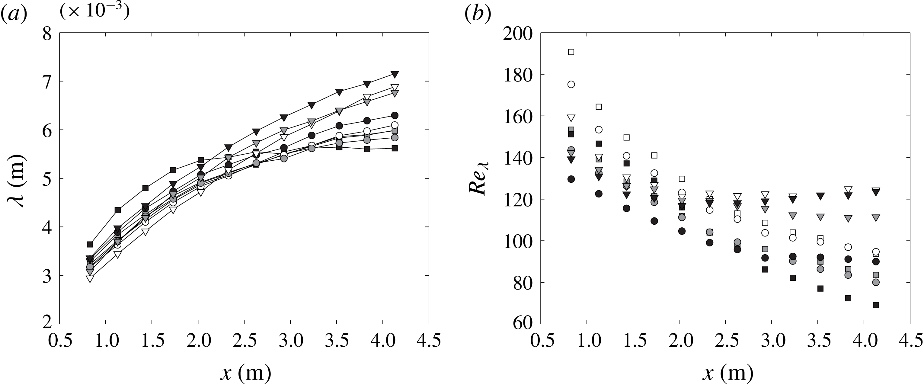
Streamwise profiles of (a) Taylor microscale
 $\unicode[STIX]{x1D706}$
, and (b) local Reynolds number
 $Re_{\unicode[STIX]{x1D706}}$
for grid 1 (square), grid 2 (circle) and grid 3 (triangle) at
 $y=0.25~\text{m}$
(white),
 $y=0.46~\text{m}$
(grey) and
 $y=0.66~\text{m}$
(black).

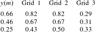
Fitted constant
 $C$
in (3.9) at selected
 $y$
locations for all grids.
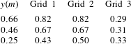
3.6 Taylor microscales
In this section we report Taylor microscale values calculated from
 $\unicode[STIX]{x1D706}=u^{\prime }/(\overline{(\unicode[STIX]{x2202}u/\unicode[STIX]{x2202}x)^{2}})^{1/2}$
. Figure 21(a) gives the streamwise development of
 $\unicode[STIX]{x1D706}$
versus
 $x$
. It can be observed that
 $\unicode[STIX]{x1D706}$
increases with
 $x$
in all cases. This agrees well with several previous experiments such as Rose (Reference Rose1966), Champagne et al. (Reference Champagne, Harris and Corrsin1970). Tavoularis & Karnik (Reference Tavoularis and Karnik1989) also showed a region
 $\unicode[STIX]{x1D70F}^{\ast }>16$
, where
 $\unicode[STIX]{x1D706}$
remains constant against
 $\unicode[STIX]{x1D70F}$
. This is not observed here due to the small mean shear rates. We also report the local Reynolds number
 $Re_{\unicode[STIX]{x1D706}}=u^{\prime }\unicode[STIX]{x1D706}/\unicode[STIX]{x1D708}$
along the
 $x$
direction, where
 $\unicode[STIX]{x1D708}$
is the kinematic viscosity. Their values decrease monotonically for grid 1 and grid 2. For grid 3, a mild increase after
 $x=2.5~\text{m}$
is observed, which corresponds to its higher turbulence intensity
 $u^{\prime }$
(see figure 8
a), and the larger value of
 $\unicode[STIX]{x1D706}$
(see figure 21
a). This is in agreement with the observation of Nedić & Tavoularis (Reference Nedić and Tavoularis2016) where they showed an increase of
 $Re_{\unicode[STIX]{x1D706}}$
after
 $\unicode[STIX]{x1D70F}^{\ast }>4.5$
.
Taylor microscale
 $\unicode[STIX]{x1D706}$
profiles for grid 1 (square), grid 2 (circle) and grid 3 (triangle) along the
 $y$
direction at
 $x=0.83~\text{m}$
(filled symbols) and
 $x=4.13~\text{m}$
(empty symbols).

Along the shear direction
 $y$
, Rose (Reference Rose1966) reported decreasing values of
 $\unicode[STIX]{x1D706}$
with increasing local mean velocity, whereas Champagne et al. (Reference Champagne, Harris and Corrsin1970) showed roughly constant values of
 $\unicode[STIX]{x1D706}$
along the shear direction. The shear rates of the two cases are similar, i.e.
 $\unicode[STIX]{x2202}U/\unicode[STIX]{x2202}y=13.6~\text{s}^{-1}$
and
 $12.9~\text{s}^{-1}$
, respectively, so it seems the shear rate is not the reason for this difference. Note however, Rose (Reference Rose1966) used wire gauze with different spacings along the shear direction as a generator, while Champagne et al. (Reference Champagne, Harris and Corrsin1970) used parallel plates with equal spacing but different local blockage ratios to generate the shear flow. There are no more data available for a more comprehensive conclusion, but the current study is similar to that of Champagne et al. (Reference Champagne, Harris and Corrsin1970), in that the layer height is constant with varying local blockage ratios, and therefore it might be expected to have a roughly constant
 $y$
-profile of
 $\unicode[STIX]{x1D706}$
. The results of the Taylor microscale
 $\unicode[STIX]{x1D706}$
along the
 $y$
direction at
 $x=0.83~\text{m}$
and
 $x=4.13~\text{m}$
are given in figure 22, and it indeed seems roughly constant.
3.7 Flow isotropy
Summary of centreline turbulence characteristics at different streamwise locations for different grids at
 $Re_{D}=8500$
based on the width of the vertical grid bar.
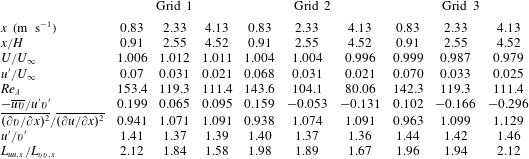
Having shown the streamwise development of turbulence intensities and length scales, we now examine the isotropy of the flow. Some of the results are given in table 5 at different
 $x$
locations along the centreline at
 $y=0.46~\text{m}$
. The small scale isotropy indicator
 $\overline{(\unicode[STIX]{x2202}v/\unicode[STIX]{x2202}x)^{2}}/\overline{(\unicode[STIX]{x2202}u/\unicode[STIX]{x2202}x)^{2}}$
seems to suggest that the flow is anisotropic as the ratio is much smaller than the isotropic value of 2, even though they are increasing along the
 $x$
direction. These results are in agreement with previous observations made by Shen & Warhaft (Reference Shen and Warhaft2000) and Schumacher (Reference Schumacher2001).
It is interesting that the results close to the grid suggest large scale isotropy of the flow such that
 $L_{uu,x}/L_{vv,x}=2$
, but
 $u^{\prime }/v^{\prime }\approx 1.4$
on the other hand. These values are maintained best by grid 3 if we compare the values at different streamwise locations in table 5. Intuitively, the shearing stress is expected to strain the large scale structure along the mean shear direction and impose anisotropy to the flow, which seems to counter our observation that
 $L_{uu,x}/L_{vv,x}=2$
. Similar observations have been reported before, for example Rose (Reference Rose1966) showed
 $L_{uu,x}/L_{uu,y}=2$
and
 $u^{\prime }/v^{\prime }\approx 1.5$
in a turbulent shear flow generated by a parallel wire grid, and Tavoularis & Corrsin (Reference Tavoularis and Corrsin1981) reported
 $L_{uu,x}/L_{vv,x}=4.34$
with
 $u^{\prime }/v^{\prime }\approx 1.4$
in a parallel plate-generated turbulent shear flow. These observations seem to suggest that the ratio of
 $L_{uu,x}/L_{vv,x}$
and
 $u^{\prime }/v^{\prime }$
reflect different aspects of anisotropy of the flow, and do not need to take their isotropic values concordantly.
Transverse profiles of (a) mean velocity
 $U/U_{\infty }$
(symbols with solid line) and
 $V/U_{\infty }$
(inset, symbols with dashed line); (b) turbulence intensity
 $u^{\prime }/U_{\infty }$
(symbols with solid line) and
 $v^{\prime }/U_{\infty }$
(symbols with dashed line) across the centre of the grid where
 $y/H=0.5$
.

3.8 Transverse homogeneity
The transverse homogeneity of the shear flow is discussed in this section. The mean velocity and turbulence intensity profiles are given in figure 23(a,b), respectively, measured at
 $x=0.83~\text{m}$
(or
 $x/H=0.91$
, open symbols) and
 $x=4.13~\text{m}$
(or
 $x/H=4.52$
, filled symbols) across the centre of the grid at
 $y=0.46~\text{m}$
or
 $y/H=0.5$
. From figure 23(a), it is observed that the transverse profiles of the streamwise mean velocity are more homogeneous closer to the grid, whereas the vertical mean velocity is more homogeneous further downstream (filled symbol with dashed line in the inset). A sinusoidal variation seems to be present for the streamwise mean velocity profiles measured at
 $x=4.13~\text{m}$
, and the profiles seem to be symmetric about the centre plane
 $z=0~\text{m}$
, although the variations are all within
 $8\,\%U_{\infty }$
. For the mean velocity profiles of
 $V/U_{\infty }$
, the sinusoidal variation is also observed symmetric about the centre plane, and the amplitude is smaller (within 5 %
 $U_{\infty }$
). The symmetry is due to the alignment of the vertical bars at
 $z=0~\text{m}$
, and might be reduced by arranging the vertical bars in a staggering pattern.
This symmetry is also observed in the transverse profiles of streamwise turbulence intensity
 $u^{\prime }/U_{\infty }$
at
 $x=0.83~\text{m}$
, as shown in figure 23(b) with open symbol and solid line. Nevertheless, the variation of the turbulence intensity is within 1 %
 $U_{\infty }$
. The transverse profiles of
 $v^{\prime }/U_{\infty }$
seems to be more homogeneous in all cases. We therefore further quantify the homogeneity of the streamwise properties in the transverse direction, referring to the criteria proposed by Corrsin (Reference Corrsin1963), namely
 $$\begin{eqnarray}\displaystyle & \displaystyle \unicode[STIX]{x2202}L_{u}/\unicode[STIX]{x2202}z\ll 1, & \displaystyle\end{eqnarray}$$
 $$\begin{eqnarray}\displaystyle & \displaystyle (L_{u}/\unicode[STIX]{x1D706})\unicode[STIX]{x2202}\unicode[STIX]{x1D706}/\unicode[STIX]{x2202}z\ll 1, & \displaystyle\end{eqnarray}$$
 $$\begin{eqnarray}\displaystyle & \displaystyle (L_{u}/\overline{u^{2}})\unicode[STIX]{x2202}\overline{u^{2}}/\unicode[STIX]{x2202}z\ll 1. & \displaystyle\end{eqnarray}$$
 $x=0.83~\text{m}$
(open symbols), and
 $x=4.13~\text{m}$
(filled symbols).
Homogeneity of the transverse profiles for grid 1 (square), grid 2 (circle) and grid 3 (triangle) at
 $x=0.83~\text{m}$
(or
 $x/H=0.91$
, open symbols) and
 $x=4.13~\text{m}$
(or
 $x/H=4.52$
, filled symbols) across the centre of the grid at
 $y/H=0.5$
.

The values of the homogeneity criteria, as shown in figure 24, are all smaller at the streamwise location closer to the grid. The values calculated at
 $x=0.83~\text{m}$
are all within
 $\pm 0.05$
as seen in figure 24(a–c). These figures suggest that the transverse homogeneity of the shear flow is better at
 $x=0.83~\text{m}$
, or
 $x/H=0.91$
, which is a nice trait as the turbulence intensity level is higher in this region.
4 Conclusions
In this paper we proposed a new class of inhomogeneous multiscale grids, and examined the turbulent shear flows generated by these grids using hot-wire anemometry. There are three major conclusions from the shear flows generated by these grids:
(i) Generation of a desired mean velocity profile is possible by optimizing the blockage ratio profile
 $\unicode[STIX]{x1D70E}_{n}$
, while maintaining a constant
 $C_{D}$
profile of the vertical bars. The drag coefficient of the vertical bars was found to affect the mean velocity profiles significantly, and it is therefore important to maintain a constant
 $C_{D}$
. The mean velocity model after Taylor et al. (Reference Taylor, Batchelor, Dryden and Schubauer1949) and McCarthy (Reference McCarthy1964) based on the local blockage ratio
 $\unicode[STIX]{x1D70E}_{n}$
was shown to agree with our measurements, with mean shear rates of
 $0.29~\text{s}^{-1}$
,
 $2.97~\text{s}^{-1}$
and
 $4.99~\text{s}^{-1}$
for grids 1, 2 and 3, respectively. The maximum possible mean shear rate generated by these grids depends on the size of the test facility as the maximum local blockage ratio is always constrained by
 $\unicode[STIX]{x1D70E}_{n}<0.4$
.
(ii) High turbulence intensities can be generated simultaneously with the desired mean velocity profile. The maximum turbulence intensities generated by the present grids are of the order of 10 %
 $U_{\infty }$
, which is much larger than those generated by previously reported passive shear generators, and it seems possible to prescribe the shape of the turbulence intensity profile. From the scalings proposed by Gomes-Fernandes et al. (Reference Gomes-Fernandes, Ganapathisubramani and Vassilicos2012), and by considering the non-uniform convection velocity, it was shown that at a streamwise location
 $x=x_{m}$
such that
 $x_{m}/x_{\ast }^{peak}>1$
(
 $x_{m}/H=0.9$
for the current cases), the
 $y$
-profiles of turbulence intensity
 $u^{\prime }(y)$
scale as
 $(u^{\prime }/U_{n})^{2}\unicode[STIX]{x1D6FD}^{2}(C_{D}w_{n}/x_{\ast ,n}^{peak})^{-1}\sim (x_{m}/x_{\ast ,n}^{peak})^{b}$
, where
 $\unicode[STIX]{x1D6FD}=2.88$
is a constant,
 $U_{n}$
is the local (in
 $y$
or equivalently
 $n$
) mean velocity and
 $b$
is a power law constant. Based on this scaling relation, it seems possible to optimize the grid geometry to produce a desired shape of turbulence intensity profile. From the mean velocity model and the scaling of turbulence intensity, a general approach to the design of multiscale inhomogeneous grids is proposed and briefly discussed in § 3.3. The methodology can be improved by adding more constraints to the optimization problem, as new results of such experiments emerge.
(iii) For a given grid, the generated turbulence field can be described using one centreline measurement along the streamwise direction and one vertical profile at
 $x/x_{\ast }^{peak}>1$
. For the current study, the proposed model successfully predicts the
 $y$
-profiles of
 $u^{\prime }$
at different
 $x$
locations up to
 $x/H\approx 2.5$
for all cases as shown in figure 20. The evolution of various flow characteristics included in the model was also studied and compared with previous literature.
There are some other interesting observations of the shear flows generated by these multiscale grids such as the spectra, as briefly discussed in the Appendix. In terms of future work, the potential of the grid design method should be explored further to establish the range of turbulent shear flows that can be produced. The special case of homogeneous turbulent shear flows could be attempted with our grid design method because of the long standing fundamental interest in such flows. Due to the small mean shear rate, the dimensionless time scale ranges from
 $\unicode[STIX]{x1D70F}=0$
to
 $2.3$
. So it is also interesting to extend the range of measurement to larger dimensionless time scale
 $\unicode[STIX]{x1D70F}$
, where the development of various turbulence characteristics and length scales could be further examined. This can be achieved by either extending the measurement distance or increasing the mean shear rate. Measurements with multiple hot-wires will also help to understand the neglected terms in the turbulent kinetic energy model. Such studies, if successful, would provide another option to design a shear flow with desired mean velocity and turbulence intensity profiles, which will benefit both fundamental studies and a wide range of practical applications.
Acknowledgements
The authors gratefully acknowledge support from Marie Curie FP7 through the MULTISOLVE project, grant number 317269. J.C.V. also acknowledges support from ERC Advance Grant 320560.
Appendix. Spectra
Turbulence spectra
 $E_{11}(k)$
at four
 $x$
locations (0.83 m, 2.13 m, 2.93 m and 3.83 m) along the centreline at height
 $y=0.46~\text{m}$
for grid 1 (a–c), grid 2 (d–f) and grid 3 (g–i), compensated for
 $\unicode[STIX]{x1D702}$
,
 $\unicode[STIX]{x1D706}$
, and
 $L$
, respectively.

The spectra for all three grids are presented here at four streamwise locations for reference, namely
 $x=1.13~\text{m}$
, 2.03 m, 2.93 m, 3.83 m. The Reynolds number is in the range of
 $70<Re_{\unicode[STIX]{x1D706}}<190$
. First of all, considering grid turbulence, the one-dimensional spectra are expected to collapse at corresponding range when normalized with
 $L_{uu,x}$
,
 $\unicode[STIX]{x1D706}$
and
 $\unicode[STIX]{x1D702}$
, respectively. Figure 25 shows the spectra measured at different
 $x$
locations along the centreline at height
 $y=0.46~\text{m}$
. It shows that the spectra collapse well in the small wavenumber range when normalized with
 $L$
, and in the large wave number range when normalized with
 $\unicode[STIX]{x1D702}$
. This is consistent with those conclusions for homogeneous isotropic turbulence.
It is also observed from figure 25 such that for all scaling methods, the quality of collapse improves from grid 1 to grid 3, and it is interesting that for grid 3, the integral length scale
 $L_{uux}$
seems to collapse the spectra at all wavenumbers. The reason for this is not exactly clear.
Turbulence spectra
 $E_{11}(k)$
at several
 $y$
locations compensated for
 $L$
at (a)
 $x=0.83~\text{m}$
, and (b)
 $x=4.13~\text{m}$
.

When the spectra of grid 3 at different
 $y$
locations are plotted together, as shown in figure 26, the collapse is not observed even when compensated using the longitudinal integral length scale
 $L_{uu,x}$
, and the difference seems to increase with streamwise distance. These observations suggests the dependency of
 $E(k)$
on the initial conditions of the grid, but this dependency cannot be quantified at the moment.