


 , where n is the flow-law exponent,
 , où n est l’exposant de la loi de comportement,
 est une moyenne de η
 bestimmt, worin n der Exponent des Fliessgesetzes,
 die effektive Scherviskosität des Eisprofiles bedeuten.
 ist ein Mittelwert für η
1. Introduction
In the flow of a glacier or ice sheet over a bed whose slope varies along the length of the ice mass, the longitudinal coupling exerted by longitudinal stress gradients has a considerable effect in modifying the flow at each point from what it would be if the local ice thickness and surface slope determined the local flow directly according to the basic flow theory that applies in the absence of longitudinal gradients (Reference NyeNye, 1952, Reference Nye1957). Observationally, this effect has been seen in actual glaciers by comparing the local slope, measured over a longitudinal interval of about one ice thickness, with the “effective slope” that would be needed to account for the observed flow with the basic no-stress-gradient theory. For example, in Blue Glacier, Washington, Reference Meier, Meier, Kamb, Allen and SharpMeier and others (1974, p. 209) found that the effective slope needed to account for the observed ice flow was nearly constant, varying over the range 5–6.5°, along a 1400 m reach of the glacier in which the local slope varied over the range 4.5–9°. In Variegated Glacier, Alaska, Reference Bindschadler, Bindschadler, Harrison, Raymond and CrossonBindschadler and others (1977, p. 188) found that the effective slope varied much less than the local slope and that a longitudinal averaging of local slope over an interval of 2–4 km was necessary to reduce the longitudinal fluctuations in average slope to a smoothness comparable to that of the effective slope.
Several theoretical treatments of glacier flow (Reference ShumskiyShumskiy, 1961; Robin, 1967; Reference BuddBudd, 1968, Reference Budd1970[a], Reference Budd1971; Reference CollinsCollins, 1968; Reference NyeNye, 1969; Reference HutterHutter, 1981; Reference Hutter, Hutter, Legerer and SpringHutter and others, 1981; Reference PatersonPaterson, 1981, p. 98 and 164; Reference Whillans and JohnsenWhillans and Johnson, 1983) have included the role of longitudinal stress gradients and have demonstrated their importance in terms of their effects on the basal shear stress over various scales of longitudinal averaging and on flow over sinusoidal bedrock topography. We felt, however, the need for a simple general formulation that would describe, at least in approximate terms, how a particular longitudinal profile of ice thickness and bed slope in an ice mass translates itself via the intervention of longitudinal stress gradients into the particular longitudinal pattern of flow that results. In the present paper we develop such a relation and apply it to field observations. This is done by extending the approach developed by Reference BuddBudd (1968), and summarized by Reference Raymond and ColbeckRaymond (1980, p. 103) and Reference PatersonPaterson (1981, p. 100), in such a way as to obtain a longitudinal flow-coupling equation that yields a description of how the longitudinal coupling in effect performs a longitudinal averaging of the influence of local slope and thickness to give the local flow. The averaging calculation can, with choice of the averaging parameters, be carried out for actual field examples and the results compared with the observed flows.
The treatment is developed at two levels: in Part I (the present paper) at a level of considerable simplification and approximation to bring out clearly and in the simplest terms the role of longitudinal stress-gradient coupling in the flow of glaciers and ice sheets, and in Part II (Reference Echelmeyer and KambEchelmeyer and Kamb, 1986) at a higher level of rigor and complexity, for quantitative application to perturbations in glacier flow caused by perturbations in ice thickness and slope of the sort that may develop due to climatic change. The theory developed in Part I is applied to field data from two valley glaciers in Part I, and to field data from ice sheets in Part V (in preparation).
2. Longitudinal Coupling of Flow by Longitudinal Stress Gradients
We consider the plane-strain flow of a wide glacier or ice sheet down a bed surface sloping in one direction. The local ice thickness h(x) and surface slope α(x) are functions of the longitudinal coordinate x measured in a coordinate system with the x-axis pointing down-stream parallel to the mean slope of the ice surface. The geometry in the flow plane is shown in Figure 1. The slope is assumed small enough to equate sin α ≈ α. If there were no effects of longitudinal strain-rate and stress gradients, and if there were no basal sliding, the “vertically” averaged flow velocity u (x-component of velocity, u, averaged over the glacier thickness from y B to y S at a given value of x; Figure 1) would be expected to depend on the basal shear stressτ B and ice thickness h according to the well-known relation (for power-law rheology)

where τ B would depend on the surface slope via

and where the constant c I depends on the flow-law parameters and n is the flow-law exponent (Reference NyeNye, 1952). If, on the other hand, the flow were by basal sliding, Equation (1) would be replaced by

where c II will be constant if the bed-roughness spectrum and extent of basal cavitation are independent of x and where the exponent m may be (n + 1)/2 or n, or possibly something between (Reference WeertmanWeertman, 1964; Reference KambKamb, 1970, p. 702).
Glacier geometry in relation to coordinate system with x-axis in the flow plane and inclined at the mean slope of the ice surface. The surface and bed slopes α and β, the surface and bed y-coordinates yS and yB. and the ice thickness h are functions of x. ū(x) is the mean flow velocity in the x direction, averaged over the ice thickness.

To find how the flow will be modified by the coupling effect of longitudinal stress gradients, we introduce, following Reference BuddBudd (1970[b], p. 23, Equation (18), the “vertically” integrated longitudinal stress-equilibrium equation

where  is the “vertically” averaged longitudinal stress deviator component. Except for omission of a term sometimes designated “T”, involving an integral of ∂
2
τxy/∂x
2, this equation is the same as or similar to what has been used by several authors (Robin, 1967, Equation (2); Reference CollinsCollins, 1968, Equation (7); Reference NyeNye, 1969; Reference BuddBudd, 1971, Equation (5); Reference PatersonPaterson, 1981, Equation (46), p. 100; Reference Hutter and ReidelHutter, [c1983], p. 258) in discussing the effects of longitudinal stress gradients. In Part III (Reference KambKamb, 1986), we give some further development in the derivation of an exact longitudinal equilibrium equation, beyond the point reached by Reference BuddBudd (I970[b]), and show how the equation reduces to Equation (4) for small angles α and β, small longitudinal curvatures dα/dx and dβ/dx, and with neglect of the T term.
In Part IV (Reference Kamb and EchelmeyerKamb and Echelmeyer, 1986), the theory in sections 2 and 3 is extended in such a way as to take into account the T term. It is shown that, although T has some definite effects on the flow, in a first approximation they do not substantially alter the results of the simple theory based on Equation (4) with omission of T.
The way in which longitudinal stress gradients couple the flow longitudinally is obtained from Equation (4) by introducing two relations between the flow and the local stresses: 1. The stress deviator is linked to the longitudinal flow gradient by

where the effective viscosity η(y) is determined by the velocity gradients via the flow law. We introduce a depth averaged viscosity η(x) that is by definition related to the longitudinal flow gradient d u /dx by

If the strain-rate ∂u/∂x were independent of depth and dominated other strain-rate contributions to the second strain-rate invariant at all depths, then η and η would be the same and would be given by

according to the standard formulation of the flow law, where N is the viscosity parameter. In fact, because of the effect of shear stress τ xy at depth, η is a function both of d u /dx and of τ B. The introduction of an “effective longitudinal viscosity” similar to η in Equations (6) or (7) has been proposed and discussed by several authors (Robin, 1967; Reference BuddBudd, 1968, p. 63; Reference CollinsCollins, 1968; Reference PatersonPaterson, 1981, p. 100 and 165; Reference Hutter and ReidelHutter, [c1983], p. 266). The η introduced by Reference Budd and JenssenBudd and Jensen (1975, p. 267) is the same as η defined in Equation (6). While Equation (7) is definitely only an approximation, Equation (6) can be considered exact, with recognition that the depth-averaged viscosity η is in fact a somewhat complicated function of τ B and d u /dx and other strain-rates in the ice column.
2. The local flow u is related to the local basal shear stress τ B by Equation (1) in the case of pure internal deformation and by Equation (3) in the case of pure basal sliding, or in general by a combination of the two. We thus introduce Equations (1) or (3) into Equation (4). Admittedly, Equations (1) and (3) are only approximations, the simplest relations between local stresses and local flow that can be written down within a framework in which the effects of longitudinal stress gradients on flow are represented as modifications that preserve the linear variation of τxv with y on which Equations (1) and (2) are based. The “constant” c I in Equation (1) is strictly a constant only if the longitudinal stress does not significantly affect the effective viscosity that controls the shear flow as a function of depth. In a more accurate approximation (Reference NyeNye, 1957), c I should be taken as a function of d u /dx and τ B, which will cause u to depart from the strict dependence on τ B n indicated in Equation (1) for constant c I. In spite of these potential complications in theory, there is empirical evidence that a relation of the type in Equation (1) is valid in the description of glacier flow (Reference Raymond and VoightRaymond, 1978, p. 812). We use Equations (1) and (3) here in the spirit of using the simplest reasonable relationships between flow and stress that exhibit the coupling effects of longitudinal stress gradients, so as to obtain a clear overview of how the longitudinal averaging of ice thickness and surface slope operates in determining the local flow.
Introducing Equations (1), (5), and (6) into Equation (4) gives, after slight re-arrangement,

Given the ice thickness h(x) and slope α(x) as functions of the longitudinal coordinate x, and given that η depends on d u /dx (as well as on τ B and therefore on u ), Equation (8) can be considered the differential equation that determines u (x) through the coupling effect of longitudinal stress gradients contained in the first term on the left. We call it the non-linear longitudinal flow-coupling equation. An equation essentially equivalent to Equation (8) was obtained by Reference BuddBudd (1968, Equation (39)) and Reference Budd and JenssenBudd and Jensen (1975, Equation (43)), but its implications for longitudinal flow coupling were not developed along the lines followed here.
For the case of basal sliding, an equation like Equation (8) applies, in which the second term on the left is replaced by ( u /c II)1/m .
3. Longitudinal Averaging of the Influence of Ice Thickness and Surface Slope on Flow
The effects of the longitudinal coupling in Equation (8) can most clearly be seen by obtaining the solution of a linearized form of this equation. Suppose that the glacier geometry and flow are a perturbation from a datum state in which Equation (1) applies exactly, namely, in which α and h are constant (α0 and h 0), independent of x, so that u = u o is also constant. We write the perturbations as ∆α = α –α0, ∆ h = h – h 0, and the resulting flow perturbation as v = ( u − u o)/ u o. When these are introduced into the second term of Equation (8), it becomes, to lowest order in the perturbations,

Introducing into the first term of Equation (8) the perturbation relation for u but not for h or η, and using the fact that the unperturbed variables satisfy Equations (1) and (2), we obtain

where ∆(αh) = αh – α 0 h 0. Note that h and η in the first term of Equation (10a) are the perturbed values, not h 0 and η o. An unusual and key feature of the perturbation treatment here is that we do not introduce the datum-state viscosity η o, which would be infinite for the datum state and flow law used. For infinitesimal perturbations, h in the first term of Equation (10a) could be replaced by h 0, but it is not necessary to do so, and it is physically more appropriate to retain the h, since it represents the well-defined role of ice thickness in the transmission of longitudinal forces along the length of the glacier. Consistent with infinitesimal character of the perturbations, the terms on the right in Equation (10a) can be combined into a single term ρg∆(αh (n+1)/n )/h 0 1/n , which can in turn be written in logarithmic form as ρgα0 h 0 ∆ln(αh 1+(1/n)). Putting τ 0 = ρgα 0 h 0 and multiplying through by n/τ0, we obtain

If now we define

and

then Equation (10b) can be rewritten in the form

where

F(x) is the logarithmic velocity perturbation that would result from a perturbation ∆h in ice thickness and ∆α in surface slope if the response were purely local according to Equations (1) and (2), without the effects of longitudinal coupling that are contained in the derivative terms in Equation (13). We call Equation (13) the linearized longitudinal flow-coupling equation. For the case of pure basal sliding, on the basis of Equation (3), n in Equations (11) and (14) is replaced by m, and the quantity +1 in the exponent in Equation (14) is omitted.
The quantity ℓ in Equation (11), which has the dimensions of length, will be called the longitudinal coupling length. It provides the fundamental length scale in the longitudinal averaging of the effects of ∆h and ∆α on the local flow.
The role of the coupling length ℓ is brought out most clearly by finding the solution of Equation (13) in the simple case where ℓ is constant, independent of x, and where the term with coefficient σ can be neglected. The solution, obtained in the Appendix, is

Equation (15) shows that the slope and thickness perturbations at each point influence the flow over a range of distances up- and down-glacier from the point, the influence dropping off exponentially with distance. The exponential decay has scale length ℓ.
The longitudinal variations of both ice thickness and surface slope enter into the longitudinal averaging by which the local flow is determined, according to Equation (15). While this is mechanically reasonable, as was pointed out by Reference Meier, Meier, Kamb, Allen and SharpMeier and others (1974, p. 210), it seems to be common practice to consider longitudinal averaging of surface slope only (Reference BuddBudd, 1968, p. 68; Reference Bindschadler, Bindschadler, Harrison, Raymond and CrossonBindschadler and others 1977 p.18).
The exponential weighting of the influence of ice thickness and surface slope on the flow, as indicated in Equation (15), is illustrated in Figure 2. It is intuitively more satisfying than the “box-car” weighting that has apparently been used up to now in taking running means of α(x) (Reference BuddBudd, 1968, fig. 3; Reference Bindschadler, Bindschadler, Harrison, Raymond and CrossonBindschadler and others, 1977, fig. 6). (“Box-car” or rectangular weighting is uniform weighting over an averaging window of chosen length, with the weight dropping abruptly to zero outside the window; see Figure 2.)
Weighting functions for longitudinal averaging. The exponential function indicated theoretically by Equation (15) is compared with triangular and rectangular weighting functions. All functions are scaled to have unit area over the interval −2ℓ ≤ x ≤ 2ℓ, which is taken as the averaging window for practical approximation of exponential weighting. With this scaling, the triangular function deviates from the exponential by the same amount at x′ – x = 0 and |x′ – x| = 2ℓ. The length 4ℓ is called the “averaging length, ” while ℓ is called the “longitudinal coupling length.”

Plot of cross-sectionally averaged effective viscosity η as a function of longitudinal strain-rate du/dx, from Equation (22). For an infinitely wide channel (curves designated f = 1), the averaging is done by Equation (6). with ∂u/∂x assumed constant in Equation (22). For a semi-circular channel (f = 1/2), the averaging is weighted by the radial distance from the channel center line, as explained in the text. For each channel type, curves are given for basal shear stress τB = 1.0 bar (solid curves) and 1.5 bar (dashed curves). The viscosity parameter N in Equation (22) is taken as 1.0 bar a1/3, and n is 3.

Comparison between effective surface slope α* calculated by longitudinal averaging (solid curve, from Equation (33). with averaging length 1.4 km) and values derived from the measured flow of Blue Glacier (data points). The dashed curve shows the local slope sin α(x) on the same scale. The solid circles are α*obs values obtained from the measured velocities and ice depths by Equation (44). The open circles and the data for α(x) and h(x) are from Reference Meier, Meier, Kamb, Allen and SharpMeier and others (1974. p. 206–09) and are plotted on the longitudinal coordinate scale x of these authors’ Figures 8 and 9 (called ξ by them). The open circles were obtained from the observed flow on the basis of a longitudinal continuity calculation in such a way that the resulting α*obs values are decreased by increasing amounts of basal sliding, whereas increased basal sliding tends to increase the α*obs values obtained from Equation (34). For x < 0.25 km the two types of data points coincide. The flow constant cI in Equation (1) is arbitrarily chosen so that the effective slope α* at x = 0.0 km equals the local slope α there.

The exponential weighting has as a consequence that the local slope (on a longitudinal scale comparable to the ice thickness) will have an effect on the local flow that is appreciable, though muted by the longitudinal averaging. This effect is often seen qualitatively in glacier flow by the opening of transverse crevasses in reaches where there is a local down-stream increase in surface slope, and in the disappearance of such crevasses where the slope decreases down-stream. A quantitative (as well as qualitative) example is seen in Blue Glacier near longitudinal coordinate ξ = 750 m (Reference Meier, Meier, Kamb, Allen and SharpMeier nd others, 1974, fig. 8), where there is a small local peak in flow velocity just where the surface slope has a local peak and where a set of transverse crevasses appears; these localized effects occur even though the peak in slope is limited to a longitudinal interval of only about 300 m, little more than the ice thickness. If the weighting of the influence of surface slope on flow were uniform over an averaging window of length several times the ice thickness, as in the box-car averaging that has been used up to now, the effects of a short reach of steep slope would be spread out uniformly over the full length of the averaging window and there would be no localized flow peak and crevassing concentrated in the short steep reach as is actually observed.
Input data for longitudinal averaging calculation of flow in Variegated Glacier. The ice thickness h(x) and surface slope α(x) in 1978, and the channel-shape factor f(x), are plotted on a longitudinal coordinate scale x where the head of the glacier is at x = 0 and the terminus is at approximately x = 20 km. Sources of the datá are given in the text. Where there is a conflict between data sources for h(x), as explained in the text, we here use the solid rather than the dotted h(x) curve as input to the longitudinal averaging calculation.

For an input perturbation that is sinusoidal in x, i.e.

the averaging integral in Equation (15) gives a flow response

which is attenuated by the factor 1/(1 + (2πℓ/λ)2) over what it would be if longitudinal averaging did not operate. The attenuation factor is 1/2 for λ = 2πℓ and drops to 0.09 for λ = 2ℓ. Thus the flow response to topographic waves of wavelength ≲ 2ℓ is strongly attentuated. An essentially full response, attentuated less than 10% by effects of longitudinal coupling, will be seen only for waves with λ ≳ 20ℓ. In the intermediate range, 2ℓ ≲ λ ≲ 20ℓ, there is partial attenuation, which means that the longitudinal fluctuations in the “slope stress” ρghα are partially supported by longitudinal stress gradients and partially by basal shear stress fluctuations. The foregoing three wavelength ranges are what emerge from the longitudinal flow-coupling theory as the short, long, and intermediate length scales of glacier motion as defined by Reference Raymond and ColbeckRaymond (1980, p. 106). The simple result of Equation (17) from longitudinal coupling theory for flow with sinusoidal longitudinal variations can be compared with related calculations by other methods, specifically those by Budd (Reference Budd1970[a], Reference Budd1971), Reference Hutter and ReidelHutter ([c1983], p. 237, fig. 4.17a), Reference Langdon and RaymondLangdon and Raymond (1978), and Reference Whillans and JohnsenWhillans and Johnson (1983). A general comparison of this kind is beyond the scope of the present paper, but a comparison with results of Reference Langdon and RaymondLangdon and Raymond (1978) will be given in Part V (in preparation).
With a rectangular weighting function (as in Fig. 2) in place of the exponential in Equation (15), the result of averaging Equation (16) would be a flow response

Superimposed on the attenuation as a function of wavelength in this case are oscillations between positive and negative response values, the negative values in the range 2ℓ < λ < 4ℓ being particularly troublesome. This unsatisfactory behavior is another practical reason in favor of the exponential averaging indicated in Equation (15).
The integration in Equation (15) is shown as extending from x′ = −∞ to +∞, as formally given by the solution in the Appendix, but in practice, obviously, the integration can extend only over the actual length of the glacier. As long as the point x is farther than a distance 2ℓ from the ends of the glacier, the effect of the finite length on the integral is negligible because of the exponential weighting function in Equation (15).
Although Equation (15) is the exact solution of Equation (13) only for ℓ constant and σ = 0, in the Appendix it is shown that the longitudinal averaging integral in Equation (15) remains a good approximation to the solution of Equation (13) when there is a longitudinal gradient in ℓ, so that σ ≠ 0, and also when there is longitudinal variation in σ. Under these conditions, ℓ in Equation (15) is the “local” value (x), dependent on x but not dependent on x′ in the averaging integral. This robustness of the form of the solution in Equation (15) against longitudinal variations of ℓ may help to explain why Equation (15) with constant ℓ is able to account fairly well for observed glacier flow (see sections 7 and 8), even though ℓ probably varies in general with x in actual glaciers, as discussed in section 5.
4. Effect Of Flow in Channel of Finite Width
By an elaboration of the procedure used in deriving Equation (13), it can be shown that for a glacier flowing in a finite-width channel whose shape is constant but whose ice-filling depth h varies with position x, the longitudinal flow-coupling equation is modified by the appearance of the channel-shape factor f that enters the well-known modified form of Equation (2)

The modification of Equation (13) consists in the following modified forms of Equations (11) and (14):


The parameter σ in Equation (12) is affected by the appearance of a factor ω:

ω is h/ h , where h is the maximum ice thickness in a cross-section and h is the thickness laterally averaged across the cross-section. Because of the f in Equation (19), the size of ℓ is affected by channel shape (see section 5). For a parabolic channel, ω = 3/2, hence the finite channel width has an appreciable effect on the parameter σ. For large σ this will introduce appreciable asymmetry into the longitudinal average, as explained in the Appendix to Part II.
Longitudinal variations in ice cross-section other than those that can be approximated as due to variation of ice-filling depth in a channel of fixed cross-sectional shape result in further modifications of Equation (13), which are beyond the scope of the present paper.
5. Longitudinal Coupling Length
The longitudinal coupling length ℓ, from Equation (19), is typically on the order of one-half to a few kilometers. The chief uncertainty in its evaluation is the value of the vertically averaged effective viscosity η, which depends, as noted earlier, on τB and d u /dx.
The simplest evaluation of η is for a shear stress τxy that increases linearly from 0 at the surface to τB at the bed, and a longitudinal strain-rate ∂u/∂x that is constant with depth. This is the model of Reference NyeNye (1957). The viscosity η(y) is given, for n = 3, as the solution of

where N is the viscosity parameter in Equation (7). Equation (22) can be obtained from Reference NyeNye (1957, Equation (26)). For a wide channel, η is a uniformly weighted average of η(y) over y
B ≤ y ≤ y
S, as in Equation (6). Values of η are shown in Figure 3, for N = 1.0 bar a1/3, n = 3, and for a typical range of longitudinal strain-rates. Values are also shown for a semi-circular channel. In this case, the viscosity distribution in Equation (22) applies approximately if ∂u/∂x is constant over the cross-section, and to calculate the cross-section-averaged η the η(y) values are weighted not by a constant as in Equation (6) but by 2(y
S – y)/h
2, where y
S – y is the radial distance from the center of the semi-circle. The approximation in using Equation (22) in this case is that it does not include the effect of strain-rate components  and (to a lesser extent)
 (z is the transverse coordinate) which, because of the particular constraint on lateral strain imposed by the semi-circular boundary, will be non-zero in this case even though
 is uniform over the cross-section; however,
 and
 are probably appreciable relative to
 only in the marginal zones, where η is dominated by the basal-marginal shear stress, hence their effect is probably small.
A useful approximation to η for a wide channel, from Equation (22), is

The approximation is good to ±1% for |d u /dx| < 0.1 a-1 when N = 1 bar a1/3 and τB = 1 to 1.5 bar, as can be checked from the values in Figure 3. For a semi-circular channel, the corresponding approximation is

It is good to ±5% for |du/dx ≲ 0.1 a-1, when N = 1 bar a1/3 and τB is in the range 1.0 to 1.5 bar, as can again be checked from Figure 3. Equations (23) and (24) for η are in general much more appropriate in normal glacier-flow situations than is Equation (7), because the longitudinal strain-rate rarely dominates the internal shear flow to the extent required for validity of Equation (7).
Figure 4 gives values of ℓ, from Equation (19), based on the η values plotted in Figure 3 and on mean flow velocity u 0 = 50 m a∲1 and ice thickness h 0 = 250 m, for wide (f = 1) and semi-circular (f = 1/2) channels.
Dependence of longitudinal coupling length ℓ on average longitudinal strain-rate <|du/dx|> for average flow velocity u 0 = 50 m a−1 and ice thickness h = 250 m. from Equation (19) with n = 3 and η as calculated in Figure 3. Curves for a very wide channel are labeled f = 1, and those for a semi-circular channel are labeled f = 1/2. Curves for basal shear stress τB = 1.0 bar are solid, those for 1.5 bar are dashed. The meaning of the angular brackets around <|du/dx|=, representing a longitudinal average, is explained in the text and will be more fully discussed in Part V, section 2.

If the flow relation in Equation (1) is introduced into Equation (19), we find that for a given τB the ratio ℓ/h will be independent of h:

Within the range of the parameters considered in Figure 4, ℓ/h ranges from about 1.5 to over 10. (In obtaining Equation (25) from Equations (1) and (19), the distinction between h 0 and h is dropped, these quantities being approximately the same for a small perturbation.)
Evaluated for the standard flow law that underlies Equations (1), (7), and (22), the coefficient c I in Equation (25) is

where the factor q is n + 2 for a very wide channel and n + 3 for a semi-circular channel. If η in Equation (25) is taken from Equation (23) for a wide channel, n being 3, then, with Equation (26),

where

The angular brackets represent an appropriate longitudinal average, as explained below. If, similarly, for a semicircular channel (f = 1/2), η is taken from Equation (24), then

Values of ℓ/h from Equations (27) and (29), over a range of longitudinal strain-rates, are shown in Figure 5 for τ B = 1 and 1.5 bar and for N = 0.7 and 1.3 bar a1/3, which approximately bracket the range of N values that have been determined from bore-hole measurements in temperate glaciers.
The parameter T that controls ℓ/h in Equations (27) and (29) is, from Equation (28), the ratio of basal shear stress to a measure of the average longitudinal deviatoric stress. In order to control correctly the effect of longitudinal stress gradient on flow, ℓ/h as obtained from Equations (19) and/or (25)-(29) should be based on an η value that is appropriately averaged longitudinally, and therefore on a correspondingly averaged value <du/dx>, which is represented by the angular brackets in Equation (28) and in Figures 4 and 5. In Part V, section 2, it will be shown that for longitudinal flow variations that are approximately sinusoidal. <|d u /dx|> is about one-third of the maximum value of |d u /dx| that occurs.
The values of ℓ/h and their variations with channel shape and longitudinal strain-rate are generally similar in Figures 4 and 5, but the dependence on basal shear stress is markedly different. The difference reflects the fact that the curves in Figure 5 are for given ice-viscosity parameters, whereas the curves in Figure 4 are for a given glacier-flow velocity (50 m a−1) and thickness (250 m). As explained below, the latter curves are more nearly appropriate if a substantial part of the flow velocity u 0 is contributed by basal sliding.
Dependence of ℓ/h on <|du/dx|> as given by Equation (27) for a wide channel (f= 1, upper curves) and by Equation (29) for a semi-circular channel (f= 1/2, lower curves). For each basal shear-stress value, a pair of curves is given, the upper curve for N = 0.7 bar a1/3, the tower for N = 1.3 bar a1/3. For τB = 1.0 bar (solid curves), the pair of curves is joined by diagonal cross-hatching to indicate the range of N values that occur for temperate glaciers. For τB = 1.5 bar (dashed curves), the curves are joined similarly by vertical hatching.

Figures 4 and 5 suggest that for temperate valley glaciers, with f near 0.5 and with longitudinal strain-rates typically of order 0.01-0.05 a−1, ℓ/h should be in the range from about 1 to 3, whereas for ice sheets, with f near 1 and with du/dx ~ 10−4 to 10−3a−1, the expected ℓ/h is in the range from about 4 to 10, distinctly higher than for valley glaciers.
The foregoing results provide a basis for considering possible variations in coupling length ℓ along the length of a given glacier. Longitudinal variation of ℓ arises from variation of the product h η in Equations (11) or (19), because the h and η there are variables of the actual, longitudinally varying flow state, rather than fixed values of the datum state, as explained in section 3. If the product h η is longitudinally variable, σ will necessarily be non-zero according to Equation (12). Figures 4 and 5 give an indication of the variations in ℓ that can be expected as a result of variations in longitudinal strain-rate along the length of a glacier. Under a given strain-rate variation, the expected percentage variation in ℓ for a valley glacier is only about half as great as for a wide ice sheet. Substantial variations in ℓ on this account are particularly to be expected in and adjacent to ice falls, where high longitudinal strain-rates occur locally.
Longitudinal variations in h probably result in little variation in l except near the terminus and head of the glacier, where h goes to zero, and, again, in ice falls, where h is small. According to Equations (11) or (19), ℓ would go to zero or become small in these places. This effect stems physically from the well-defined role of the ice thickness in transmitting longitudinal forces along the length of the glacier, expressed in the first term of Equation (4). In the approximation represented by the perturbation treatment here, ℓ varies as  from Equations (11) or (19). However, this approximation is not good in the places where h becomes small, because there the perturbation from a datum state appropriate to the glacier as a whole is not small. Nevertheless, to the extent that the perturbation treatment remains valid in a rough way, an effect of the kind stated, in which ℓ goes to zero as h does, is intuitively reasonable and can be expected. There is perhaps room for the intuitive conjecture that in these places the effective ℓ might go to zero more nearly as h than as
 If so, it would be behaving more as indicated in Equations (25), (27), (29), and (32), rather than as in Equations (11) or (19) by the strict requirements of the perturbation treatment.
The last two paragraphs indicate that the assumption that ℓ does not vary longitudinally, which underlies the strict derivation of the longitudinal averaging integral in Equation (A-15) in the Appendix, is only an approximation. The effects of longitudinal variations in ℓ on Equation (A-15) are considered in the Appendix and in section 9, and further in the Appendix to Part II.
In the case of flow by internal deformation of isotropic ice, the velocity
u
o in Equation (19) arises by flow under the same viscosity field η(y) that determines
η
, from Equation (22) or the approximate Equations (23) or (24). This is, of course, the basis for Equation (26) and the consequent relations for ℓ/h in Equations (27) and (29). To bring out this point in a more general way, we can define an average viscosity  via a double average of the reciprocal effective viscosity η(y), linearly weighted, as follows:

To the approximation that τ xy (y) is a linear function of y, as in the treatment of Reference NyeNye (1957), the integral in Equation (30) is what arises in the calculation of the average velocity u from the shear flow.Footnote * In fact,

Equations (22), (30), and (31) constitute a restatement of the flow Equation (1), incorporating Equation (1) as a special case when c
I is strictly constant, and also allowing for the more general flow equation that can arise within the framework in which τxy
is a linear function of y and ∂u/∂x is independent of y; these features characterize the theory of glacier flow without longitudinal stress gradients (Reference NyeNye, 1957) and will also apply rigorously to flow with a longitudinal stress gradient when that gradient is independent of y. The factor 3 in Equation (30) is introduced so that when η is a constant,  Equations (30) and (31) allow us to recast ℓ from Equation (19) in the simple and fundamental form

where  is given by Equation (30) and where, if the longitudinal strain-rate ∂u/∂x is independent of depth,
η
is the Simple average of η(y) over the thickness h as in Equation (6) or over the channel cross-section as discussed above for a semi-circular channel.Footnote
†
η
may be called the “effective longitudinal viscosity” and
 the “effective shear viscosity” for the flow.
Note that the distinction between the effective longitudinal and shear viscosities, from Equations (6) and (30), is not based on any assumptions about viscous anisotropy, although such anisotropy probably contributes to lowering  because of the strong ice-crystal fabric of basal ice. A shear-viscosity quantity essentially equivalent to
 was introduced by Reference BuddBudd (1968, Equation (37)), who considered that the shear flow governed by
 could be strongly non-linear (n ~ 3), while the longitudinal flow governed by
η
was approximately linear (Reference BuddBudd, 1968, p. 67). Because
η
in Equations (23) and (24) is dependent on du/dx, however, the contemplated linearity is questionable.
In the case of flow by basal sliding only, n is replaced by m in Equation (19), according to Equation (3). On this account, the coupling length might be shortened slightly (20% or so). On the other hand, sliding increases u
0 over what it would be for internal deformation only, and this augments ℓ, according to Equation (19). This augmentation helps to explain why ℓ/h for actual temperate valley glaciers (sections 7–9) is somewhat larger than the values shown in Figure 5 for the relevant du/dx range of about 0.01 to 0.05 a −1. An extreme instance of this augmentation is in a surging glacier. For the lower part of Variegated Glacier under surge in June 1983, when the flow velocity was u
0 ≈ 50 m d−1, with h ≈ 330 m, τB≈ 1.5 bar, and
η
~ 0.65 bar a (estimated from Equation (24) with d
u
/dx ~ 2 a −1), the value of ℓ indicated by Equation (19) is ~ 4 km, or ℓ/h ~ 12. This long coupling length, which is about one-quarter the length of the glacier, helps to explain why time variations in velocity were similar at widely spaced points up- and down-stream (Reference Kamb and KambKamb and others, 1985, fig. 5). A surging or rapidly sliding glacier has an abnormally low value of the effective shear viscosity  , which in this case is not given by Equation (30) but instead by Equation (31) with u being determined by the mechanics of basal sliding.
6. Dependence of Coupling Length on Flow-Law Exponent
The ratio  in Equation (32) increases with n, because the weighted average of η(y) in Equation (30) gives enhanced weight to the low values of η that occur near the bed when the flow law is non-linear. For this reason, as well as the factor n in Equation (32), the longitudinal coupling length for non-linear flow is longer than for linear flow. This was in effect pointed out, though not in terms of the coupling length ℓ explicitly, by Reference Raymond and ColbeckRaymond (1980, p. 108) in interpreting the results of calculations of the effects of longitudinal stress gradients on flow in an idealized ice sheet. For n = 1, and consequently
η
=
 , Equation (32) (with f = 1) indicates that the ratio ℓ/h has the fixed value 1.15. For n = 3, Figure 5 indicates that at typical longitudinal strain-rates in ice sheets, ℓ/h ~ 7. This large value of ℓ/h is confirmed by a more detailed theoretical treatment and by evaluation of field data for ice sheets in Part V.
7. Effective Slope from Longitudinal a Veraging: Comparison of Theory with Field Examples
The applicability of the theory in sections 3–5 can be tested by comparing the effective surface-slope values α*obs that have been obtained from the observed flow in some glaciers with values calculated from Equation (15). For this purpose Equation (15) is recast as follows. The theoretical effective slope α* is the value of α that, when used in Equations (1) or (3) in conjunction with the local thickness h, reproduces the local velocity required theoretically by Equation (15). Thus, in the case of Equation (1), for a small perturbation

where v is given by Equation (15) and where we take α0 to be the local value of α. If we also take h 0 to be the local value of h, and take

consistent with small perturbations, then we can convert Equation (15) to the form

where h 0 = h(x) and f 0 = f(x) in accordance with the datum-state specification above. In the case of basal sliding only, from Equation (3), the 1/n in the exponents in Equation (33) is to be dropped.
In carrying out numerically the longitudinal averaging in Equation (33) we can replace the exponential weighting function to a good approximation by a triangular function of length 4ℓ, shown in Figure 2. We will call the length 4ℓ of the triangular averaging window the longitudinal averaging length, as distinct from the “longitudinal coupling length” ℓ defined in section 3.
In Figure 6 are given the results of applying Equation (33) (with the exponential replaced by triangular weighting) to data from Blue Glacier, Washington (Reference Meier, Meier, Kamb, Allen and SharpMeier and others, 1974, fig. 8). The dashed curve is α(x), and the heavy curve is α*(x) obtained from Equation (33) with the 1/n in the exponents omitted and with longitudinal variation of f ignored. Omitting the 1/n is equivalent to assuming that the flow is mainly by basal sliding, but it is done here not for this reason but just for simplicity in calculation and because for n = 3 it makes little difference anyway. The averaging length used is 4ℓ = 1.4 km, which is about 6–7 times the ice thickness.
The open circles in Figure 6 are  values calculated from flux continuity by Reference Meier, Meier, Kamb, Allen and SharpMeier and others (1974, table V). The solid circles are
 values that reproduce the observed velocities u
obs when used in Equation (2) together with the equation for the surface velocity corresponding to Equation (1); thus

The effective slope  defined by Equation (34) in conjunction with Equation (1) is the same quantity as the “basal friction coefficient” introduced by Reference BuddBudd (1968, Equation (11)). The representation of the flow in terms of the effective slope in effect subsumes under α* the effects of longitudinal variations in ice thickness and cross-sectional shape factor as well as in surface slope. To obtain from Equation (34) the
 values plotted in Figure 6, the constant c
I is evaluated at x = 0 by taking
 = α there; n is taken to be 3.
The calculated α *(x) curve in Figure 6 follows the solid circles rather well, except near the terminus, where difficulty would be expected anyway (see section 9). The open circles follow a pattern similar to the α*(x) curve but drifting away from it down-glacier. This drift reflects increasing contributions from basal sliding, which are implied by the flux-continuity calculation (Reference Meier, Meier, Kamb, Allen and SharpMeier and others, 1974, p. 206–10). The peak in flow velocity mentioned in section 3, at x = 0.7 km, is matched by a peak in α* there, both as obtained from Equation (33) and as calculated from the observed flow velocity by Equation (34).
In Figure 7 is the result of similarly applying Equation (33) to data from Variegated Glacier, Alaska (Reference Bindschadler, Bindschadler, Harrison, Raymond and CrossonBindschadler and others, 1977). The averaging length used is 4ℓ = 2.0 km. The  points in Figure 8 are obtained from the f
v sin αv values of Reference Bindschadler, Bindschadler, Harrison, Raymond and CrossonBindschadler and others (1977, fig. 6) by dividing by the shape factor f, which is obtained from a smooth curve drawn through the squares and triangles given in these authors’ Figure 7. The longitudinal averaging by Equation (33), with variation of f again ignored, gives an α*(x) curve that accounts for the details (local peaks and troughs) in the pattern of observed
 points better than do the rectangular averages calculated by Reference Bindschadler, Bindschadler, Harrison, Raymond and CrossonBindschadler and others (1977, fig. 6). In particular, the peak in the α*(x) curve at x = 10.7 km falls where there is a marked local maximum in flow velocity and an 0.5 km reach of prominent transverse crevassing. The rectangular averages of Reference Bindschadler, Bindschadler, Harrison, Raymond and CrossonBindschadler and others (1977) do not show a peak at this location.
Effective surface slopes for Variegated Glacier. Observed values, obtained as explained in the text, are shown by points connected by a heavy curve. The local surface slope, sin α(x), is shown with a dashed curve. The data are from Bindschadler and others (1974, figs 6 and 7) and are plotted on the longitudinal coordinate scale of these authors. The thin solid curve shows α* values calculated by longitudinal averaging of α(x) via Equation (33) with the exponential approximated by triangular weighting (fig. 2). and with averaging length 2.0 km.

The above example reveals an unsatisfactory feature of the effective surface-slope values  as indicators of the effects of longitudinal coupling on flow: the
 data of Figure 8 give only a weak indication of the flow-velocity peak at x = 10.5 km, whereas this is one of the most prominent and distinctive features of the observed flow curve (Fig. 9b). This shortcoming is rooted in the fact that the
 values are much more sensitive to the local thickness h than they are to the local flow velocity u, as Equation (34) indicates. Variations in h, real or imagined (from observational error), that are not closely linked to variations in
u
in the way that Equations (1) and (2) require will show up much more strongly in the
 (x) values than the variations in u(x) that we are actually interested in.
Comparison of observed flow of Variegated Glacier in 1977–78 with flow calculated by the longitudinal coupling theory from the data in Figure 8. (a) Flow velocity uL(x) from Equations (1) and (2) based on local α(x) and h(x) without longitudinal averaging. (b) Flow velocities u(x) calculated by longitudinal averaging from Equations (35) with the triangular weighting function of Figure 2, for averaging lengths 4l = 2.0 km (dashed curve), 2.5 km (fine solid curve), and 4.0 km (dotted curve). The observed flow uobs(x) is shown by the heavy solid curve with data points, and is from Reference Raymond, Raymond, Harrison, Gitomer, MacQueen, Senear and MacKeithRaymond and others (unpublished). The calculated u(x) curves are matched to uobs at x = 9.5 km. (c) Flow velocities calculated by rectangular averaging of surface slope only, from Equations (36). for averaging lengths of 2.5 km (solid curve) and 4.0 km (dotted curve). The curves are matched to uobs at x = 9.5 km.

8. Comparison of Observed Flow with Flow Predicted by Longitudinal Coupling Theory for Variegated Glacier, Alaska
In examining the effects of longitudinal averaging on flow, it is therefore more informative to look at the flow velocity directly rather than its representation in terms of an effective slope α*(x) from Equations (33) or (34). We here compare the observed surface-velocity curve u obs(x) for Variegated Glacier with theoretical curves u(x) calculated from Equation (15) with use of observational data for α(x) and h(x).
The calculated curves are obtained in the following way. The logarithmic slope and thickness values are averaged to give a quantity A as follows:

For the Variegated Glacier data we use as the weighting function W ℓ(x) in Equation (35a) the triangular function in Figure 2. The integral in Equation (35a) is carried out as a discrete sum over data points at a spacing of ∆x’ = 0.25 km. By comparing Equation (15) with Equation (35a), in which the ∆ operator does not appear, and noting that ∆lnαnfnhn+1 = lnαnfnhn+1- lnαn 0fn 0h0 n+1, we see that A(x) given by Equation (35a) is v + lnα0 n f0 nh0 n+1, calculated with a practical limit of ±2l on the range of integration. Therefore, for small perturbations, for which ln(u(x)/u 0) = ln(l + v)≈ v, from Equation (35a) we obtain

where x 0 is an arbitrary reference point along the length of the glacier. Hence we calculate u(x) from

u(x) is thus matched to the observed velocity at the reference point x = x 0, which in effect evaluates c I in Equation (1) there. Since Equation (15) as it stands gives u rather than the surface velocity u s, we assume, consistent with the basis for Equations (1) and (2), that uS/ u is a fixed ratio (n + 2)/(n + 1) and thus simply scale up u from Equation (15) to calculate the surface velocity by Equation (35b). The exponential form of Equation (35b) in a sense restores the flow non-linearity from the linearizing approximation made in Equation (9). In what follows, we use n = 3 throughout.
The results of the above procedure applied to data for Variegated Glacier (fig. 8) are given in Figure 9. The data set α(x) is derived from the profile of surface elevations along the glacier center line at 0.25 km intervals measured in September 1978 by Reference Raymond, Raymond, Harrison, Gitomer, MacQueen, Senear and MacKeithRaymond and others (unpublished). The data set h(x) is obtained from the ice thickness as measured in 1973–74 by Reference Bindschadler, Bindschadler, Harrison, Raymond and CrossonBindschadler and others (1977, fig. 2), adjusted by the change in surface elevation between 1973 and 1978 measured by Reference Raymond, Raymond, Harrison, Gitomer, MacQueen, Senear and MacKeithRaymond and others (unpublished), and modified in the x intervals 0–9 km and 16–20 km as shown by the difference between the solid curve and dotted curve in Figure 9. The modifications are based on our knowledge of ice thickness at x = 3.0, 6.5, 8.8, 9.5, and 11.8 km from bore holes drilled to the bottom in 1978–80 and 1982, and on radio echo-sounding at x = 3.2 and 3.5 km in 1981 and over 16–18 km in 1983. For x < 3.0 km, we make a reasonable extrapolation of h(x) toward the head of the glacier at x = 0 km. The data set u obs(x) (Fig. 9b) consists of the annual velocities measured from July 1977 to July 1978 by Reference Raymond, Raymond, Harrison, Gitomer, MacQueen, Senear and MacKeithRaymond and others (unpublished). The match point is taken at x 0 = 9.5 km. The curve of values for the shape factor f (fig. 8) is obtained from Reference Bindschadler, Bindschadler, Harrison, Raymond and CrossonBindschadler and others (1977, fig. 6) as explained in section 7 above, and extrapolated up-glacier from km 6.
Figure 9a shows the flow uL(x) that would occur if longitudinal averaging did not operate and if the flow were governed by the local α and h via Equations (1) and (2). The curves labeled 2, 2.5, and 4 in Figure 9b show the calculated u(x) that results from longitudinal averaging, via Equation (35) with averaging length 4l = 2.0, 2.5, and 4.0 km, respectively. The effect of longitudinal averaging in suppressing the wild oscillations in the uL(x) curve of Figure 9a is dramatic, and confirms the large attenuation expected for the flow response to short-wavelength variations in α(x) as discussed in section 3. The best choice of the averaging length 4l is about 2.5 km, based on the observationally required smoothness of u(x) and on the way the velocity peak centered at x = 10.5 km is accounted for in Figure 9b.
The calculated u(x) curves account fairly well for the observed u obs(x) (Fig. 9b) from about Km 14 up-glacier to about Km 5. The detail in the u obs(x) curve between Km 5.5 and 6.5 is probably the result of the entrance of a main tributary over this interval (see Reference Bindschadler, Bindschadler, Harrison, Raymond and CrossonBindschadler and others, 1977, p, 187). Since this causes violations of the simple assumptions on which Equation (15) is based, it is not surprising that the theoretical u(x) curve does not reproduce the detail in the u obs(x) curve there.
But up-stream from Km 5.5 a major discrepancy between u(x) and develops. There is no way to account theoretically for the high peak at Km 4.5 with any choice of the averaging length 4ℓ .It appears to us that over the interval Km 5.5 to 3.0, and perhaps up to about 2.0, a major component of flow velocity, amounting to ~10-20 cm d−1, is added over and above what would be expected on the basis of the flow characteristics of the glacier below Km 7. This added component is probably an extra contribution from basal sliding. It is very significant, we think, that this large extra contribution occurred in just the reach where in 1982 the surge of the glacier began (Reference Kamb and KambKamb and others, 1985), and where in previous years the flow events called “mini-surges” developed (Reference Kamb and EngelhardtKamb and Engelhardt, in press).
The calculated u(x) curves in Figure 9b include the effect of longitudinally varying shape factor f. There is a large effect only below Km 16, where f increases markedly down-stream (fig. 8) as the valley widens. Without the effect of f, the u(x) curves diverge below uobs(x) from Km 12 onward. Even with the effect of f, there is some divergence beyond Km 14.
To compare the results of our approach with the type of longitudinal averaging that has been considered previously, in Figure 9c we show velocity curves calculated on the basis of longitudinal averaging of surface slope only, using a rectangular (“box-car”) averaging window. The calculation is done in a manner analogous to Equations (35a) and (35b) as follows. The slope is averaged logarithmically to give

with 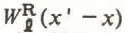 being the rectangular weighting function shown in Figure 2, and the velocity is calculated from

The factor involving h(x) in Equation (36b) arises because of the dependence of u on local h required by Equation (1) when only longitudinal averaging of α is considered. The velocity curves labelled 2.5 and 4 in Figure 9c are calculated in this way for averaging lengths of 2.5 and 4.0 km. These curves give a much poorer representation of u obs (x) than do the curves calculated by our method (Fig. 9b).
9. Calculated and Observed Flow of Blue Glacier, Washington, Including The Role of Basal Sliding
Figure 11 shows the results of applying the longitudinal averaging procedure of Equation (35) to the data in Figure 10 for Blue Glacier, Olympic Mountains, Washington (Reference EchelmeyerEchelmeyer, unpublished). The match point is taken at x = 0.06 km on the longitudinal coordinate scale of Figures 6, 10, and 11 (which corresponds to ξ = 1180 m on the longitudinal coordinate scale used by Reference EchelmeyerEchelmeyer (unpublished)). The curve u L(x) (Fig. 11a) is the flow velocity that the local thickness h(x) and slope α(x) would generate, if they controled the flow locally according to Equations (1) and (2). The actual velocity curve u obs(x) is shown in Figure 11b, and is compared there with calculated curves u(x) from longitudinal averaging with lengths 4l of 1.2, 1.8, and 2.4 km. The weighting function W ℓ(x′ – x) used in calculating these curves by Equation (35) is the exponential shown in Figure 2, truncated at the limits x′ – x = ±2ℓ. From Figure 9b it is clear than an averaging length of 1.2 km is in general too short, and 2.4 km is too long. The peak in u obs(x) around x = −0.3 km can be fitted reasonably well by 4ℓ = 1.8 km, To reproduce the peak near x = 0.7 km requires a shorter 4l, about 1.5 km, as would be expected from Equation (25) because the ice is thinner there (see fig. 10). To calculate in a rough, simple way the effect of a possible decrease in l toward the terminus, we suppose that 4l decreases from 1.8 km at x = 0.2 km to 0.6 km at x = 1.7 km, and represent it over this interval by its average, 1.2 km. In addition, we bring into consideration the asymmetry in the longitudinal averaging that enters when there is a longitudinal gradient in ℓ, as noted in section 4. Following Part II, section 3, this is done by using two separate averaging lengths in Equation (35), 2ℓ − = 0.75 km for x′ < x, and 2ℓ + = 0.45 km for x′ x, corresponding to ϵμ ≈ 0.25 in Equation (17) of Part II. The averaging interval runs from x′ = x − 2ℓ − to x′ = x + 2ℓ +, with total length 2ℓ − + 2ℓ + = 1.2 km. Similarly, where the ice thins up-stream toward the ice fall, asymmetric averaging is again used, with 2ℓ − = 0.7 km, 2ℓ + = 1.1 km. This modification in the longitudinal averaging calculation, the result of which is shown in Figure 11c, gives a velocity peak at x = 0.7 km in rough agreement with the observed peak.
Ice thickness h(x) and surface slope α(x) for the lower part of Blue Glacier, in 1977–78, from Reference EchelmeyerEchelmeyer (unpublished). The longitudinal coordinate x is the same as in Figure 6. The ice fall in the upper part of the glacier extends down to about x = −1.2 km. From about x= 1.5 to 2.0 km is the steep terminal front.

Comparison of observed flow of Blue Glacier in 1977–78 with flow calculated by the longitudinal coupling theory from the data in Figure 10. (a) Flow velocity uL(x) calculated by Equations (1) and (2) from the local slope α(x) and thickness h(x) without longitudinal averaging, (b) Flow-velocity curves u(x) calculated by symmetrical longitudinal averaging from Equations (35) (with the truncated exponential weighting of Figure 2) for averaging lengths 4ℓ = 1.2 km (dashed curve), 1.8 km (fine solid curve), and 2.4 km (dotted curve). The observed velocities uobs(x) are shown by the heavy solid curve with data points. The calculated velocities are matched to uobs at x = 0.06 km. (c) Flow velocity u(x) calculated by longitudinal averaging with longitudinally variable and asymmetric coupling lengths, as follows: x < −0.5 km, 2ℓ − = 0.7 km, 2ℓ + = 1.1km; −0.5 < x < 0.2 km, 4ℓ = 1.8 km; 0.2 < x < 1.7 km, 2ℓ − = 0.75 km, 2ℓ + = 0.45 km. (d) u(x) modified from (c) by introduction of large sliding-velocity contributions in the ice fall (x < −1.1 km) and near the terminus (x > 1.2 km) as described in the text. The observed uobs(x) is again shown for comparison.

Beyond about x = 0.9 km, the calculated curve u(x) drops greatly below the observed velocity. This is due to the influence of the terminal region of the glacier; in the calculation, the rapid thinning of the ice down-stream from x = 1.1 km dominates over the increase in α(x) there, resulting in a calculated velocity that decreases rapidly down-stream. The discrepancy here probably reflects increasing contributions from basal sliding as the terminus is approached. It is known that the sliding component is less than about 10% of the total annual motion in the middle part of the glacier, x ~ −0.8 to +0.8 km (Reference Engelhardt, Engelhardt, Harrison and KambEngelhardt and others, 1978; Reference EchelmeyerEchelmeyer, unpublished), whereas it increases both in absolute and relative amount near the terminus as indicated by measurements of marginal sliding there (Reference Meier, Meier, Kamb, Allen and SharpMeier and others, 1974, p. 198).
Up-stream from x = −0.9 km the observed velocity shows a strong up-swing, which is not followed by the calculated u(x) curves in Figure 11b. This reach is the lower part of a large ice fall that heads the glacier; it is evident in Figure 10 in terms of the high slopes and low ice thicknesses for x ≲ −1.2 km. The high velocities there are due to rapid basal sliding, amounting to as much as 130 ma−1, which was observed at the head of a tunnel driven to bedrock (Reference Kamb and LaChapelleKamb and LaChapelle, 1968; Reference KambKamb, 1970, p. 706, example 4).
The amount of internal deformation flow observed in the tunnel, 30 m a−1, is approximately what is calculated at x ≲ −1.2 km in Figure 11a and b, indicating that the theory based on Equation (1) accounts roughly for the flow due to internal deformation even under the extreme conditions in the ice fall. The reduction in the amount of internal deformation flow in the ice fall stems from the fact that the somewhat increased τ B there (increase of 15–25%) is more than offset by the effect of the greatly reduced ice thickness via the factor h in Equation (1).
For the longitudinal coupling theory to take into account the large flow contribution from basal sliding in the ice fall and near the terminus, a source term that represents this contribution needs to be added to the right-hand side of Equation (13). To do this by including a contribution to u from Equation (3) would necessitate making the factor c II in Equation (3) be a function of x that expresses the change in sliding contribution from a large amount in the ice fall to a small or negligible amount below the ice fall, with little change in τ B. A simple approximate way of doing this is to add to F(x) as given by Equation (14) the x-dependent quantity In(l+u B/u 0) where u B/u 0 represents the ratio of basal sliding to internal deformation flow. The same quantity then appears as an addition to the existing source term in the longitudinal averaging integral in Equations (15) and (35). Just as in the case of the localized extra sliding contribution to Variegated Glacier noted in section 7, the x-dependent variation of u B /u 0 must occur for reasons beyond the scope of longitudinal coupling theory as formulated here, hence the theory provides no a priori way of prescribing it. An a posteriori, ad hoc, and therefore “not-to-be-recommended-for-general-use” way of doing it simply for illustrative purposes is to treat u B/u 0 as an x-dependent “fudge factor” and to adjust it to improve the match between calculated and observed u(x). Figure 11d shows the result of doing this in the following simple way. For the utmost simplicity (doubtless an oversimplification), we take u B/u 0 to be a step function with constant value 5.5 in the ice fall, dropping abruptly to zero at x = −1.1. To represent similarly the sliding contribution near the terminus, we add a second-step function, for which u B/u 0 jumps from 0 to 4.5 at x = +1.2 and is constant from there to the terminus. The parameters ℓ, ℓ +, and ℓ − are the same as for the curve in Figure 11c. As expected, this ad hoc procedure for including a sliding contribution in the longitudinal averaging calculation makes a distinct improvement in the agreement in Figure 11d between u(x) and u obs(x) in and adjacent to the reaches where sliding is known to be important.
The quasi-exponential tail of decreasing velocity u(x) from x = -1.1 km, where the assumed input contribution from sliding terminates, to about x = −0.8 km is the direct effect of a large longitudinal stress gradient in the lower part of the ice fall, by which the high velocities in the ice fall extend their influence down-stream over a distance of the order of the coupling length. We would expect ℓ to be relatively short here because η should be relatively small in the reach of large longitudinal compression near the base of the ice fall. (In the calculation for Figure 11d the value ℓ − that controls the down-glacier influence of the ice fall is 0.35 km.)
The large increase in basal sliding toward the terminus makes it difficult to judge exactly how important the effects of decreasing l and the associated asymmetry in longitudinal averaging are in bringing forth the peak in flow velocity near x = 0.7 km, which is where the surface slope has a pronounced local maximum as discussed in sections 3 and 7. The velocity peak, in terms of effective slope values α, was obtained in section 7 by longitudinal averaging with 4ℓ = 1.4 km, only slightly different from the average value 2ℓ ℓ + 2ℓ + = 1.2 km used in calculating u(x) in Figure 11c; thus there is a general consistency between the two approaches. On the other hand, a gentler, more distributed decrease in ℓ toward the terminus, as specified below, Footnote * one that seems reasonable in relation to u(x) there, generates a u(x) curve little different from the one for 4ℓ = 1.8km in Figure 11b, with no peak at x = 0.7 km. We could say that the observed velocity peak at x = 0.7 km definitely requires the more rapid decrease in ℓ around x = 0.2 km, were it not for the fact that the large increase in sliding velocity toward the terminus might also somehow be involved in producing the peak.
10. Effect of Longitudinal Coupling on Basal Shear Stress
Because many previous discussions of the subject have concentrated on how the basal shear stress is modified from the “slope-stress” value (given in Equations (2) or (18)) by the effects of longitudinal stress gradients, as summarized by Reference Raymond and VoightRaymond (1978, p. 808, 1980, p. 104) and Reference PatersonPaterson (1981, p. 100), and also because in ice-sheet-flow modeling it is a common practice to formulate ice-flow velocity in terms of a direct relation to basal shear stress (e.g. Reference LingleLingle, 1984, Equation (6)), we indicate here how the results of the longitudinal flow-coupling theory developed in the present paper are expressible in terms of the effect of longitudinal coupling on basal shear stress. This is obtained simply by combining the result of Equation (15) with Equation (1), or, in the case of basal sliding only, with Equation (3). The most attractive form of the combination is obtained if we choose for the datum state h 0, α 0 the local h(x) and α(x) at a point x where the basal shear stress is to be calculated. From Equations (1) and (2), u 0 is then related to the local “slope stress” τL for simple shear (“laminar flow”) by

In this case, the introduction of Equations (15) and (1) into Equation (9), in which now ∆h = 0 at x (but not in general at x’≠ x) because of the chosen datum state h 0 = h(x), gives

Introducing τL(x′) = ρgα(x′)h(x′), based on Equation (37), into the integrand in Equation (38), we can express the result as

The first term on the right can be included within the integral, and the ∆ operation expanded to first order, giving

Since by definition of the ∆ operation

the above relation simplifies to

where the quantity h outside the integral is h(x).
The form of Equation (39), which is closely related to Equation (33), shows that the effect of longitudinal stress gradients on the basal shear stress can be obtained by an exponentially weighted longitudinal averaging of the local slope stress τL, the exponential scale length being the longitudinal coupling length ℓ. The local thickness h(x′) also enters the weighting factor in the averaging, but weakly, because of the exponent ℓ/n. If basal sliding dominates, then the factors h 1/n in Equation (39) are to be omitted.
The effect of the T term on the relationship in Equation (39) is discussed in Part IV.
11. Conclusions
Because the longitudinal coupling theory in sections 2 and 3 is developed on the basis of the linearization in Equation (9), which approximates longitudinal variations in the flow of an ice mass as small perturbations upon an overall average flow, the theory should work best under conditions where the longitudinal variations in ice thickness and surface slope are small. Part V will provide an idealized test of this situation, and shows that the theory tests out rather well. In actual glacier-flow situations for which longitudinal variations in ice thickness and slope are not small perturbations, one might not expect the theory to give more than a rough approximation to the observed flow. Nevertheless, the foregoing comparisons between observations and calculations show that in the parts of Blue Glacier and Variegated Glacier where the flow is dominated by internal deformation, the theory is able to account reasonably well for the longitudinal variations in flow (sections 8 and 9) or for their representation in terms of effective slopes (section 7). This is accomplished with a coupling length l that is for the most part longitudinally constant in each glacier. In Blue Glacier, we seem to have an example of a situation in which a decrease in ℓ toward the terminus has a noticeable effect. In handling such a situation for a valley glacier, the longitudinal averaging becomes asymmetric, according to the theory developed in Part II.
The averaging lengths (4ℓ) that achieve the best match between calculated and observed velocities (or effective slopes) for Blue Glacier and Variegated Glacier lie in the range 1.2–2.5 km, corresponding to ℓ/h ≈ 1.5–2.5, h being the ice thickness. This falls within the range of theoretical ℓ/h values for semi-circular channels in Figures 4 and 5, for longitudinal strain-rates in the range 0.01–0.05 a−1, which are typical for these glaciers. In Figure 5, the predicted range of ℓ/h values for semi-circular channels at strain-rates of 0.01–0.05 a−1 is somewhat low, but three factors tend to increase ℓ/h toward the value c. 2 that is actually observed: (1) the effective longitudinal strain-rate <du/dx> to be used in Figure 5 is reduced from the maximum center-line values by a factor of about 0.2, because of averaging over the cross-section (factor ≈ (n + l)/(n + 3)) and longitudinally (factor 0.3, see section 5 and Part V); (2) the actual channel shapes are intermediate between semi-circular and very wide; (3) a significant fraction of the flow may be by basal sliding, which, as explained in section 5, raises ℓ/h over the values calculated in Figure 5.
A large flow contribution from basal sliding in the Blue Glacier ice fall and near the terminus makes itself evident as a large excess of the observed velocity over what is given by the longitudinal averaging calculation in these reaches. When the calculation is modified in an ad hoc way to include a sliding contribution, the results show how the high sliding velocities in the ice fall are felt in attenuated form below the ice fall to distances of order ℓ through the action of a large longitudinal stress gradient there.
In Variegated Glacier before surge, a major excess of observed over calculated velocity in 1977–78 is found in the very reach of the glacier where the 1982 surge later started, implying that an abnormally large amount of basal sliding was occurring in this reach prior to the surge.
Acknowledgements
This work was supported by National Science Foundation grants EAR-50-08319 and DPP-82-09824. Permission of the U.S. National Park Service and U.S. Forest Service for the field work that obtained data in sections 6–8 is acknowledged. We thank K. Hutter for valuable criticisms.
Appendix
Solution of Differential Equation for Longitudinally Coupled Flow
Equation (13) is of the form

where ˄ x is the second-order linear differential operator

The second form of ˄ x in Equation (A-2) follows from Equations (11) and (12) if n, u 0, and τ 0 are constant, as they are in the perturbation treatment here, in which case σ is given simply by

The reason for replacing σ by the symbol μ at this point will be explained in Part II.
Equation (A-2) shows that the operator λ x is self-adjoint (Reference Courant and HilbertCourant and Hilbert, 1931, p. 298; some authors call this “formally self-adjoint”), and from the theory of differential equations (Reference Courant and HilbertCourant and Hilbert, 1931, p. 302; Reference StakgoldStakgold, 1979, p. 194) it is known that for homogeneous boundary conditions on v(x) the solution of Equation (A-1) can then be written

Here G(x|ξ) is the Green’s function for the problem, which is the function that satisfies the differential equation

over the given interval x 1 ≤ x≤ x 2 and also satisfies the same homogeneous boundary conditions placed on v(x) at the boundaries x = x 1and x 2. In Equation (A-5), δ(x) is the Dirac delta function. Equation (A-5) implies that G satisfies the homogeneous equation

everywhere in x 1≤ x≤ x 2 except at x = ξ, and also that the function G(x|ξ), which must be continuous at x = ξ, satisfies the first-derivative “jump condition” there:

If ℓ is constant and therefore σ = 0 in Equation (A-2), then Equation (A-6) can be solved at once, giving solutions of the form

or linear combinations thereof. Different linear combinations are required for x ≤ ξ and for x ≥ ξ, in order that G satisfy the jump condition in Equation (A-7). If the boundaries are allowed to recede to large distances (±∞), the required homogeneous boundary conditions become G → 0 as x → ±∞>, and in this case the positive and negative exponentials, without combination, are the proper forms of G for x ≤ ξ and x ≥ ξ, respectively:

If we now choose a+ and a_ so that G is continuous at x = ξ and satisfies Equation (A-7), we find

When Equation (A-10) is put into Equation (A-4), and ξ replaced by x’, we get the solution quoted in Equation (15). The subscript o on G 0 in Equation (A-10) is a reminder that this is the Green’s function for μ = σ = 0.
Although the application of homogeneous boundary conditions at infinitely remote boundaries (x 1→−8, x→2 −8) seems somewhat arbitrary and unrealistic in relation to actual glacier-flow problems, it is the natural condition to apply in the perturbation treatment under consideration, since this is based on a datum state with constant u 0, h 0, and α0 extending indefinitely in x. However, it is readily possible to give a solution on a finite interval x 1, x 2 with boundary values v 1 and v 2 prescribed at x 1 and x 2. This is done by the methods given by Reference Courant and HilbertCourant and Hilbert (1931, p. 305) or Reference StakgoldStakgold (1979, p. 197, equation (2.16)), The Green’s function in this case has four exponential terms, one of which, the lead term, has the form of Equation (A-10) with a multiplicative factor near 1. As long as x is farther from x 1 and x 2 than a distance 2l, all of the other terms are reduced by a factor smaller than e −2, regardless of the value of ξ, so that the Green’s function reduces to Equation (A-10) to a good approximation. To the solution in Equation (A-4) there are added eight exponential functions of x, whose coefficients depend on the boundary values v 1 and v 2; of these functions, the lead terms have the form

and, as expected, die off exponentially from the boundaries with scale length ℓ.Thus, as long as the “point of observation”, x, is farther from the boundaries than 2ℓ, the finite-interval boundary-value solution reduces for practical purposes to Equation (A-4) with Equation (A-10). In the present treatment we content ourselves with this simple practical result, recognizing that near the terminus or head of a glacier, within a distance of ~2ℓ, a more complicated boundary-value problem must in principle be dealt with, and that in these regions the perturbation treatment will probably apply poorly, because the longitudinal variations in flow are probably not small. These same or similar considerations apply equally to the more complicated situation where ℓ varies with x, as discussed below.
The effect of longitudinal variation in ℓl on the Green’s function can be evaluated to a first approximation by considering a linear variation, corresponding to a constant gradient μ from Equation (A-3):

Since ℓ is a non-negative quantity, the form in Equation (A-11) restricts the solution space to x ≥ −ℓ0 /μif u > 0 or x ≤ −ℓ0/μ if μ < 0. If we make the variable change

(where z is restricted to have the sign of μ) then ℓ = μz and, from Equations (A-6) and (A-2), G must satisfy

This has solutions of the form

where a is a constant and p satisfies

so that

If we take the boundary conditions G = 0 at z = 0, and G → 0 as μz → +∞ (valid for either sign of μ), Footnote * then since P+ > 0 and p_ < 0, the form of G (x|ξ) that, analogously to Equation (A-9), follows from Equation (A-13) can be written

where the subscripts + apply for μz≤ μζ, the subscripts -for μz ≥ u ζ. (Including μ in these inequalities makes them correct for either sign of μ.) Following Equation (A-12) we write ζ = ξ + l0/μ. Applying Equation (A-7) and the continuity condition to evaluate a ± in Equation (A-16), we obtain

where the upper subscripts apply for μz≤μζ, the lower for μz ≥μζ. This form exhibits the (z, ζ) symmetry of the Green’s function, G(z|ζ) = G(ζ/z), which is a consequence of the self-adjoint character of λ x . Such symmetry is also shown by Equation (A-10).
Since p+ + p_ = -1, we can rewrite Equation (A-17) in the form

where the subscript + applies for μζ≤ μz, the subscript -for μζ≥ μz. This shows that, as a function of ζ, G depends only on the ratio ζ/z. For a given value of μ, the function G(ζ/z) has a fixed form, and is scaled with z in accordance with the z on the left side of Equation (A-18). A complete picture of the range of Green’s functions for various values of μ and all possible values of z is therefore obtained by evaluating Equation (A-18) as a function of ζ /z. The result is shown in Figure 12. It is given in terms of the quantity  , which has for convenience in plotting been scaled by a factor κ so that

Exact Green’s functions G(z|ζ) of the longitudinal flow-coupling Equation (13). for l a linear function of x with longitudinal gradient dl/dx = μ. = σ. The curves  , for five different values of μ, are calculated as functions of ζ /z from Equation (A-18), and are scaled relative to G(z/ζ) by the condition in Equation (A-19) for convenience in plotting. The longitudinal coordinate ζ or z is taken relative to an origin at the point where l = 0, as indicated by Equations (A-11) and (A-12).

In Figure 13 we compare G(ζ/z) from Equation (A-18) with the exponential Green’s function G
0 in Equation (A-10), calculated with l chosen to be the value at ζ = x (or ζ = z), namely, l = μz. The comparison is made in terms of  values, scaled by Equation (A-19) in both cases. (This scaling corresponds to putting a reasonable limit on the range of x or z over which the Green’s function is used in a practical calculation, beyond which the function is small; it is analogous to scaling to unity the integral of the weighting function in Equation (15) over the averaging length indicated in Figure 2. Scaling the integral in Equation (A-19) to 2μmakes the peak heights of
 sub-equal in such a way that the peaks nest nicely in Figure 12.)
Comparison between the exact Green’s function  (ζ) from Equation (A-18) (dotted curve) and the symmetric exponential
 from Equation (A-10) (solid curve), for three values of μ, both functions being scaled by the same integral condition in Equation (A-19).The value of l used in Equation (A-10) for each curve
 is μz, which is the value of l at the point z. Note that the abscissa scale for μ. = 1/4 is different from that for μ = 1/2 and 1. Also shown is
 (dashed curve), the asymmetric exponential discussed in Part II, scaled also by Equation (A-19).

The agreement in Figure 13 between  from Equation (A-18) and
 from Equation (A-10) is reasonably good, even for μ as large as 1, which is large compared to a maximum practical value of μ, about 0.3 (see Part II, section 3). The agreement increases as μ decreases. By using the form of G given in Equation (A-20), it is readily shown that as μ → 0, G(x|ξ) → G
0(x|ξ).
Figures 12 and 13 may be taken to show the behavior of the Green’s function in the neighborhood of the terminus (at z = 0) or of a deep minimum in ℓ (which could be taken at some small value of z; see below). A more general situation in the longitudinal stress equilibration of glaciers would be where ℓ has the local value ℓ0 at some arbitrary point, say x = 0, and varies linearly with slope μ about that point, as expressed in Equation (A-11). To describe this typical situation, it is useful to transform from z back to x, by Equation (A-12). G then becomes

where the upper subscripts apply for μ≤ ξ μ x, the lower for μ≥ ξμx. Designating the quantity 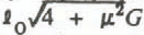 by
 , Figure 14 gives Green’s functions G(x|ξ) from Equation (A-20), for μ = 0.25. They are shown as functions of? /l0 for the particular choices x/lo = -2.6, -1.0, +1.0, and +2.5. Also shown for comparison are symmetrical exponential functions G
0(x|ξ), from Equation (A-10), with ℓ for each function taken to be the constant value l(x) as given by Equation (A-ll) for the particular value of x for that curve.
Exact Green’s function for μ = 1/4, represented by the dotted curves, which give  as a function of ξ for four values of x/ℓ0. The quantity Ğ plotted is
 , calculated from Equation (A-20); for x/ℓ0 = - 2.6, the quantity plotted is ½Ğ, scaled down for graphical convenience. Also shown, by the solid-line curves, are symmetric exponentials from Equation (A-10), scaled so as to have the same peak heights as the exact Green’s function, and with l for each curve taken to be ℓ(x) = ℓ0 + μx for the corresponding value of x/ℓ0 as indicated.

Figure 14 shows the expected broadening and flattening of the Green’s function in response to the increase in ℓ with increasing x. Moreover, it indicates again that the symmetric exponential function G 0 gives a reasonably good representation of the actual Green’s function G.
It thus appears that the Green’s function for longitudinal averaging in glacier flow is affected in only a simple way by longitudinal gradients in the coupling length ℓ. The weighting function G(x|ξ), viewed as a function of ξ for any particular value of x, is to a good approximation of a symmetric exponential with scale length equal to the local value, at x, of the coupling length, ℓ(x).
The effect of non-constant μ (non-zero d2l/dx 2) on the Green’s function can be assessed in a rough way by obtaining the Green’s function in the neighborhood of an “angular minimum” in ℓ, represented by ℓ(x) = l0 + μℓ xℓ, with μ > 0, the minimum being at x = 0. This can readily be treated by the methods used above, with the result

When G from Equation (A-21) is evaluated and compared with the symmetric exponential G 0 = exp(−|ξ|/ℓ 0), the agreement is fairly good for μ ≲ 0.5. Better agreement is obtained with a symmetric exponential of increased scale length ℓ1, where approximately ℓ1 /ℓ0 1 + 0.5μ. The increase in ℓ1 is due to the effect of the increase in ℓ(x) away from the minimum. Since over the interval −2ℓ 0 < x < +2ℓ 0 the gross curvature is roughly d2 ℓ/dx 2~ μ/2l 0, we can conclude that the effect of d2 ℓ/dx 2 is to modify the exponential scale length to

While this is a definite effect, for μ ≲ 0.5 it seems small in relation to the roughness of the underlying approximations of the theory.
Our conclusion from the above discussion is that in most situations where ℓ varies with x an adequate approximation to the Green’s function in Equation (A-4) is a symmetric exponential, as in Equation (15), with ℓ being the “local” value of the coupling length, ℓ(x), treated as constant in the integral over x’ in Equation (15). The conclusion is reasonably robust against non-zero d2 ℓ/dx 2, but if d2ℓ/dx 2 is large, a “curvature correction” in Equation (A-22) to the local ℓ can be applied as indicated in the previous paragraph.
The only situation where the above conclusion is likely to break down is for points x near a deep minimum in l(x). Figure 12 gives an idea of how the Green’s function will behave in such a place; it will be distinctly suppressed relative to the symmetric exponential as it approaches the minimum, particularly if the effective μ is ℓ or larger (which is unlikely). In this situation the weighting function given by Equation (A-20) can be used as a better approximation than the symmetric exponential in Equation (14). For this practical purpose Equation (A-20) is more conveniently written

where μ = dℓ/dx and where the subscript + applies for μ≤ ξ μx, the subscript –for μ≥ ξ μx, p ± being given by Equation (A-15).
For valley glaciers, as noted in section 4, the Green’s function is in principle somewhat asymmetric if μ ≠ 0. This is explained in the Appendix to Part II.



