2. Trajectory equations

We briefly summarize the equations, already introduced by Jenkins & Valance (Reference Jenkins and Valance2014), that govern the periodic saltating motion of a sphere of diameter $d$ and mass density ${\it\rho}^{s}$ over a horizontal bed. A turbulent shearing flow of a fluid of mass density ${\it\rho}^{f}$ and molecular viscosity ${\it\mu}^{f}$ drives the flow in the presence of gravity, with $g$ the gravitational acceleration. The horizontal velocity of the turbulent fluid is $U$ , and the horizontal and vertical components of the particle velocity are ${\it\xi}_{x}$ and ${\it\xi}_{y}$ , respectively. We assume that the flow is steady and uniform, so that the velocities are functions of only the vertical distance from the bed $y$ . 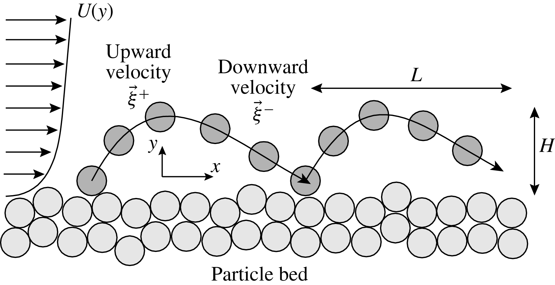The flow configuration is depicted in figure 1.

Figure 1.

Sketch of the periodic trajectory.

We characterize the particles through the fall particle Reynolds number $\mathit{Re}={\it\rho}^{f}\sqrt{g({\it\sigma}-1)/{\it\sigma}}d^{3/2}/{\it\mu}^{f}$ , where ${\it\sigma}={\it\rho}^{s}/{\it\rho}^{f}$ is the density ratio. All quantities are made dimensionless using the diameter and mass density of the particle and the reduced gravitational acceleration $g({\it\sigma}-1)/{\it\sigma}$ . We characterize the drag exerted on the particles through a nonlinear drag coefficient, which is, in dimensionless form,

(2.1) $$\begin{eqnarray}C_{D}=\frac{0.3}{{\it\sigma}}\sqrt{(U-{\it\xi}_{x})^{2}+{\it\xi}_{y}^{2}}+\frac{18}{\mathit{St}},\end{eqnarray}$$

where $\mathit{St}={\it\sigma}\mathit{Re}$ is a Stokes number. In the following, we use the superscripts $+$ and $-$ to label quantities in the upward and downward parts of a trajectory, respectively.

The upward and downward components of the particle velocity are governed by

(2.2) $$\begin{eqnarray}\displaystyle & \displaystyle {\it\xi}_{y}^{+}\frac{\text{d}{\it\xi}_{x}^{+}}{\text{d}y}=C_{D}^{+}(U-{\it\xi}_{x}^{+}), & \displaystyle\end{eqnarray}$$

(2.3) $$\begin{eqnarray}\displaystyle & \displaystyle {\it\xi}_{y}^{+}\frac{\text{d}{\it\xi}_{y}^{+}}{\text{d}y}=-1-C_{D}^{+}{\it\xi}_{y}^{+}, & \displaystyle\end{eqnarray}$$

and

(2.4) $$\begin{eqnarray}\displaystyle & \displaystyle {\it\xi}_{y}^{-}\frac{\text{d}{\it\xi}_{x}^{-}}{\text{d}y}=C_{D}^{-}(U-{\it\xi}_{x}^{-}), & \displaystyle\end{eqnarray}$$

(2.5) $$\begin{eqnarray}\displaystyle & \displaystyle {\it\xi}_{y}^{-}\frac{\text{d}{\it\xi}_{y}^{-}}{\text{d}y}=-1-C_{D}^{-}{\it\xi}_{y}^{-}, & \displaystyle\end{eqnarray}$$

respectively. The horizontal coordinates $x^{+}$ and $x^{-}$ are functions of the vertical coordinate $y$ ,

(2.6) $$\begin{eqnarray}{\it\xi}_{y}^{+}\frac{\text{d}x^{+}}{\text{d}y}={\it\xi}_{x}^{+}\end{eqnarray}$$

and

(2.7) $$\begin{eqnarray}{\it\xi}_{y}^{-}\frac{\text{d}x^{-}}{\text{d}y}={\it\xi}_{x}^{-}.\end{eqnarray}$$

The average particle velocity $u$ and the particle shear stress $s$ are

(2.8) $$\begin{eqnarray}u\equiv \frac{c^{+}{\it\xi}_{x}^{+}+c^{-}{\it\xi}_{x}^{-}}{c^{+}+c^{-}}\end{eqnarray}$$

and

(2.9) $$\begin{eqnarray}s\equiv -(c^{+}{\it\xi}_{y}^{+}{\it\xi}_{x}^{+}+c^{-}{\it\xi}_{y}^{-}{\it\xi}_{x}^{-}),\end{eqnarray}$$

where $c$ is the particle concentration. In steady uniform saltation, the vertical mass fluxes of ascending and descending particles must balance at any point, and must be independent of the vertical position. Hence,

(2.10) $$\begin{eqnarray}c^{+}{\it\xi}_{y}^{+}=-c^{-}{\it\xi}_{y}^{-}={\it\phi}_{0},\end{eqnarray}$$

where ${\it\phi}_{0}$ is the vertical mass flux at the bed. The upward flux is sometimes referred to as the pick-up function.

The fluid shear stress, $S$ , is the difference between the dimensionless fluid shear stress far from the bed, $S^{\ast }$ (the Shields parameter) and the particle shear stress: $S=S^{\ast }-s$ . In this paper, we restrict our attention to hydrodynamically rough beds. So, upon employing Prandtl’s mixing length hypothesis, the horizontal velocity of the turbulent fluid is given in terms of $S$ by

(2.11) $$\begin{eqnarray}\frac{\text{d}U}{\text{d}y}=\frac{({\it\sigma}S)^{1/2}}{{\it\kappa}(y+y_{0})},\end{eqnarray}$$

where ${\it\kappa}=0.41$ is Kármán’s constant and $y_{0}$ is the dimensionless roughness length, here taken to be $1/30$ (van Rijn Reference van Rijn1984; Jenkins & Valance Reference Jenkins and Valance2014). The assumption that the bed is rough requires that $\mathit{Re}({\it\sigma}S^{\ast })^{1/2}$ be larger than 70 (Gersten & Schlichting Reference Gersten and Schlichting2000); then the thickness of the viscous sublayer is much smaller than the particle diameter.

The system of equations (2.2)–(2.7) and (2.11) permits the determination of the seven unknowns ${\it\xi}_{x}^{+}$ , ${\it\xi}_{y}^{+}$ , ${\it\xi}_{x}^{-}$ , ${\it\xi}_{y}^{-}$ , $x^{+}$ , $x^{-}$ and $U$ , after the application of seven boundary conditions. The latter are the kinematic relations $x^{+}(0)=0$ , $x^{-}(0)=L$ , $x^{+}(H)=x^{-}(H)$ , ${\it\xi}_{x}^{+}(H)={\it\xi}_{x}^{-}(H)$ and ${\it\xi}_{y}^{+}(H)={\it\xi}_{y}^{-}(H)=0$ , where $H$ and $L$ are the height and the length of the periodic particle trajectory, and the no-slip condition $U(0)=0$ . When two further boundary conditions are introduced, the trajectory height and length can be determined as part of the solution. Experiments and numerical simulations (Oger et al. Reference Oger, Ammi, Valance and Beladjine2005; Beladjine et al. Reference Beladjine, Ammi, Oger and Valance2007; Crassous, Beladjine & Valance Reference Crassous, Beladjine and Valance2007) have shown that the particles rebound at a bumpy bed according to

(2.12) $$\begin{eqnarray}{\it\xi}_{0}^{+}=e{\it\xi}_{0}^{-},\end{eqnarray}$$

where the subscript 0 indicates evaluation at the bed, and

(2.13) $$\begin{eqnarray}{\it\xi}_{y0}^{+}=-e_{y}{\it\xi}_{y0}^{-},\end{eqnarray}$$

where ${\it\xi}\equiv \sqrt{{\it\xi}_{x}^{2}+{\it\xi}_{y}^{2}}$ is the magnitude of the particle velocity. In the absence of significant damping due to the presence of a viscous fluid, $e\equiv a-b\sin {\it\theta}$ and $e_{y}\equiv a_{y}/\sin {\it\theta}-b_{y}$ , in which $a$ , $b$ , $a_{y}$ and $b_{y}$ are numerical constants that depend on the coefficients of normal restitution and sliding friction of the particles and whether the bed is rigid or erodible (Oger et al. Reference Oger, Ammi, Valance and Beladjine2005; Beladjine et al. Reference Beladjine, Ammi, Oger and Valance2007; Crassous et al. Reference Crassous, Beladjine and Valance2007) and ${\it\theta}$ is the angle between the bed and the incident trajectory: $\tan {\it\theta}\equiv -{\it\xi}_{y0}^{-}/{\it\xi}_{x0}^{-}$ . In what follows, we use $a=0.87$ , $b=0.72$ , $a_{y}=0.30$ and $b_{y}=0.15$ for the impact of spheres both on a rigid bumpy bed and on a three-dimensional bed of like spheres (Beladjine et al. Reference Beladjine, Ammi, Oger and Valance2007). Also, we indicate the modifications of these expressions to account for viscous dissipation in the way suggested by Yang & Hunt (Reference Yang and Hunt2006), and already implemented to predict collisional sediment transport (Berzi & Fraccarollo Reference Berzi and Fraccarollo2013). In this case, the coefficients of restitution are assumed to depend on the Stokes number, so that

(2.14) $$\begin{eqnarray}{\it\xi}_{0}^{+}=e{\it\xi}_{0}^{-}-\frac{62(1+e)}{\mathit{St}}\end{eqnarray}$$

and

(2.15) $$\begin{eqnarray}{\it\xi}_{y0}^{+}=-e_{y}{\it\xi}_{y0}^{-}-\frac{62(1+e_{y})}{\mathit{St}}.\end{eqnarray}$$

For saltation over rigid bumpy beds, there are no additional conditions, so that the solution is determined by the specification of two control parameters: the Shields parameter $S^{\ast }$ and the upward flux ${\it\phi}_{0}$ . The latter can equivalently be replaced by the mass hold-up, as in Jenkins & Valance (Reference Jenkins and Valance2014), by the horizontal particle flux $Q={\it\phi}_{0}L$ , as in the experiments (Ho et al. Reference Ho, Valance, Dupont and Ould El Moctar2011), or by the vertical velocity after the rebound ${\it\xi}_{y0}^{+}$ , the take-off velocity, as in the present work. In any case, there is a range of possible particle fluxes that can be steadily sustained at a given strength of the fluid flow.

For saltation over erodible beds, experiments (Meyer-Peter & Müller Reference Meyer-Peter and Müller1948; Creyssels et al. Reference Creyssels, Dupont, Ould El Moctar, Valance, Cantat, Jenkins, Pasini and Rasmussen2009) and numerical simulations (Durán et al. Reference Durán, Andreotti and Claudin2012) show that there is only one particle flux associated with a given Shields parameter, no matter what the density ratio. In the formulation of the periodic boundary-value problem that means that there is an additional constraint that permits the determination of the upward flux – or equivalently the horizontal particle flux – as part of the solution. Trajectories over erodible beds often involve both the rebound of the colliding particle and the ejection of others. Collision experiments with a single particle show that there is a critical impact velocity, ${\it\xi}_{c}$ , below which there is only rebound and no ejection (Oger et al. Reference Oger, Ammi, Valance and Beladjine2005; Beladjine et al. Reference Beladjine, Ammi, Oger and Valance2007; Crassous et al. Reference Crassous, Beladjine and Valance2007). Hence, in order to have steady saltation over erodible beds, no incoming particle velocity can exceed ${\it\xi}_{c}$ , with the latter roughly equal to 40 (Beladjine et al. Reference Beladjine, Ammi, Oger and Valance2007). In the case of a uniform distribution of impacting velocities less than ${\it\xi}_{c}$ , the average value of the impacting velocities must be less than ${\it\xi}_{c}/2$ . Jenkins & Valance (Reference Jenkins and Valance2014) were indeed able to reproduce the experiments on aeolian saltation over erodible beds using the additional constraint that the impacting velocity of their periodic trajectory was always equal to ${\it\xi}_{c}/2$ . We will show how the assumption of a range of impact velocities less than ${\it\xi}_{c}/2$ permits the prediction of the qualitatively different relationships between the horizontal particle flux and the Shields parameter in aeolian and aquatic transport over erodible beds.

Finally, we note that the critical impact velocity depends on the amount of energy transferred and dissipated in successive collisions between the particles in the bed that are initially at rest and in contact with each other (Ho et al. Reference Ho, Dupont, Ould El Moctar and Valance2012). When an interstitial fluid is present, we assume that it does not play a role in determining the value of  ${\it\xi}_{c}$ .

3. Approximate analytical solution: periodic saltation over a rigid bumpy bed

Periodic trajectories over a rigid bumpy bed exist for a range of impact velocity. So, as already mentioned, in order to determine the numerical solution to the periodic trajectory over a rigid bumpy bed, we must prescribe both the Shields parameter and another parameter that quantifies the flow of particles in the system. Here, we take this to be the take-off velocity. This choice, although formally correct, might seem unusual, because the take-off velocity cannot be controlled in a physical experiment. However, the parametrization of the problem in terms of the take-off velocity permits the significant insight that the periodic particle trajectories and the fluid shear stress at the bed are essentially independent of the Shields parameter, which enters only in the determination of the particle shear stress and concentration.

3.1. Single particle trajectories

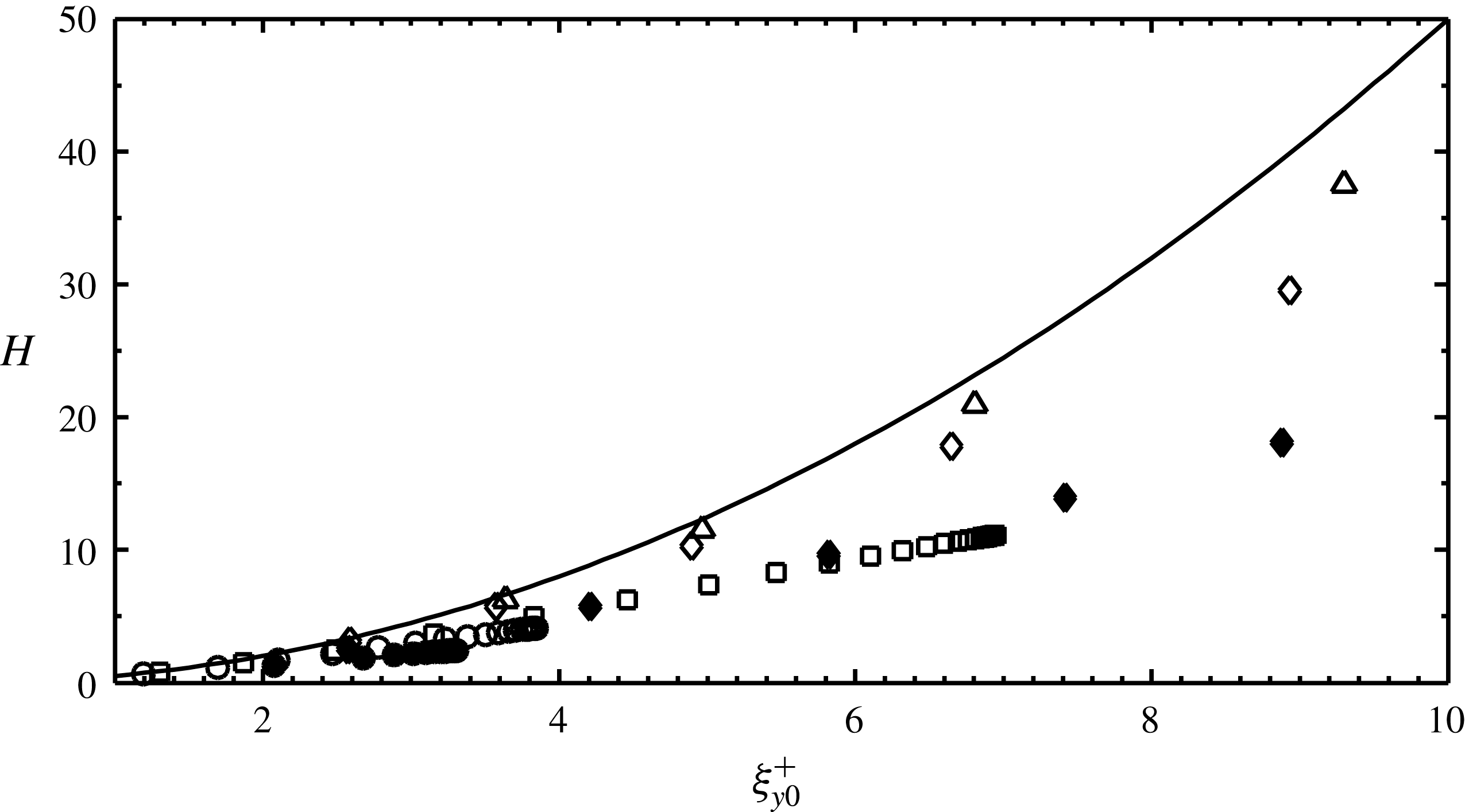
We first determine the steady periodic trajectories that are compatible with the rebound relations (2.14) and (2.15). If we assume that the vertical velocity after the rebound is so small that the drag in the vertical momentum balances can be neglected, the trajectory height is simply

(3.1) $$\begin{eqnarray}H={\textstyle \frac{1}{2}}({\it\xi}_{y0}^{+})^{2},\end{eqnarray}$$

and the downward vertical velocity before impacting the bed is

(3.2) $$\begin{eqnarray}{\it\xi}_{y0}^{-}=-{\it\xi}_{y0}^{+}.\end{eqnarray}$$

Figure 2 shows the results of the numerical integration for the periodic trajectories at different values of the Stokes number and density ratio obtained for different values of the Shields parameter. Equation (3.1) gives the upper envelope of the numerical results – the height is maximum when the vertical drag is negligible. We note that the vertical drag causes a significant reduction in the heights of the trajectories from that of (3.1) for small density ratios, Stokes numbers less than 1000 and take-off velocities larger than five.

Figure 2.

Trajectory height versus take-off velocity obtained from numerical solutions of the periodic trajectories: $\mathit{St}=1000$ (hollow symbols) and $\mathit{St}=100$ (solid symbols), when ${\it\sigma}=5$ (circles), ${\it\sigma}=10$ (squares), ${\it\sigma}=100$ (diamonds) and ${\it\sigma}=1000$ (triangles). The solid line is the approximate analytical solution of (3.1).

For Stokes numbers as large as several hundred, we can ignore the dependence of the coefficients of restitution on the Stokes number, so that $e_{y}=1$ , $\tan {\it\theta}\simeq \sin {\it\theta}\simeq a_{y}/(1+b_{y})$ and

(3.3) $$\begin{eqnarray}{\it\xi}_{x0}^{-}=\frac{1+b_{y}}{a_{y}}{\it\xi}_{y0}^{+}=A{\it\xi}_{y0}^{+}.\end{eqnarray}$$

For arbitrary values of the Stokes number, $e_{y}$ is determined from (2.15) as indicated in appendix A. For large Stokes numbers, the impact velocity is, from (3.2) and (3.3),

(3.4) $$\begin{eqnarray}{\it\xi}_{0}^{-}=\left[\left(\frac{1+b_{y}}{a_{y}}\right)^{2}+1\right]^{1/2}\!{\it\xi}_{y0}^{+}\equiv B{\it\xi}_{y0}^{+}.\end{eqnarray}$$

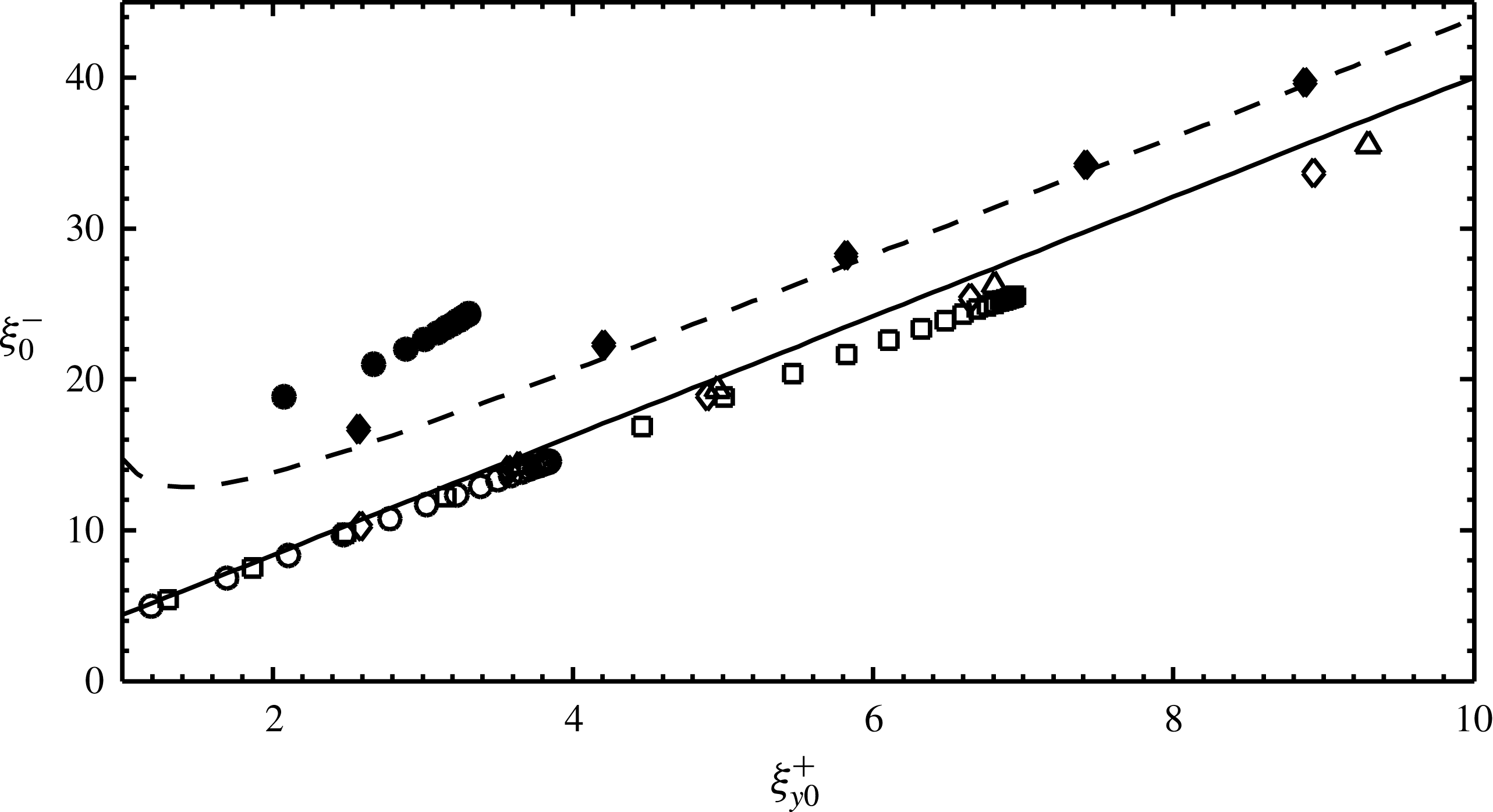
Figure 3 shows the comparison between the numerical solutions for the periodic trajectories for different values of the Shields parameter and the impact velocity predicted by (3.4). The latter reproduces the numerical results for Stokes number larger than several hundred, with no influence of the density ratio. When the Stokes number is 100, there is a departure of the numerical results from the analytical prediction; this is associated with the influence of the viscosity on the rebound. When this effect is included in the approximate analytical solution (appendix A), the agreement is also good when $\mathit{St}=100$ . For small Stokes numbers, the dependence of the numerical results on the density ratio is due to the vertical drag (figure 2). Finally, when the effect of the viscosity is included in the rebound relations, the impact velocity has a minimum, and this minimum increases with the Stokes number.

Figure 3.

Absolute value of the impact velocity versus take-off velocity obtained from the numerical solutions for the periodic trajectories. The symbols are the same as in figure 2. The solid line is the analytical approximation in the limit of large Stokes number of (3.4); the dashed line is the analytical approximation with the dependence on the Stokes number retained (A 5).

From (2.14) and (3.4), the absolute value of the velocity after the rebound ${\it\xi}_{0}^{+}$ is, for large Stokes numbers,

(3.5) $$\begin{eqnarray}{\it\xi}_{0}^{+}=\left(a-b\frac{a_{y}}{1+b_{y}}\right)\left[\left(\frac{1+b_{y}}{a_{y}}\right)^{2}+1\right]^{1/2}\!{\it\xi}_{y0}^{+}\equiv C{\it\xi}_{y0}^{+}.\end{eqnarray}$$

Hence, the horizontal particle velocity after the rebound is

(3.6) $$\begin{eqnarray}{\it\xi}_{x0}^{+}=\left\{\left(a-b\frac{a_{y}}{1+b_{y}}\right)^{2}\left[\left(\frac{1+b_{y}}{a_{y}}\right)^{2}+1\right]-1\right\}^{1/2}\!{\it\xi}_{y0}^{+}\equiv D{\it\xi}_{y0}^{+}.\end{eqnarray}$$

3.2. Fluid velocity

We next integrate the horizontal particle momentum balances, assuming that the fluid velocity is equal to its depth-averaged value over the trajectory height $\bar{U}$ . Equation (2.4) may then be rewritten as

(3.7) $$\begin{eqnarray}\frac{\text{d}{\it\xi}_{x}}{\text{d}t}=\frac{0.3}{{\it\sigma}}(\bar{U}-{\it\xi}_{x})^{2}+\frac{18}{\mathit{St}}(\bar{U}-{\it\xi}_{x}).\end{eqnarray}$$

where $t$ is time, and we have taken $\bar{U}-{\it\xi}_{x}\gg {\it\xi}_{y}$ . Upon integrating,

(3.8) $$\begin{eqnarray}\frac{\bar{U}-{\it\xi}_{x0}^{+}}{\bar{U}-{\it\xi}_{x}}\,\frac{0.3(\bar{U}-{\it\xi}_{x})/{\it\sigma}+18/\mathit{St}}{0.3(\bar{U}-{\it\xi}_{x0}^{+})/{\it\sigma}+18/\mathit{St}}=\exp \left(\frac{18}{\mathit{St}}t\right).\end{eqnarray}$$

The uniform fluid velocity is determined from (3.8), using (3.3) and (3.6), and the fact that the time of flight in a ballistic trajectory is equal to $2{\it\xi}_{y0}^{+}$ . It is worth noting that large Stokes numbers do not affect the collisions with the bed, but do influence the fluid velocity. For Stokes numbers as large as several hundred, the approximate result is

(3.9) $$\begin{eqnarray}\bar{U}=\frac{A+D}{2}{\it\xi}_{y0}^{+}+E,\end{eqnarray}$$

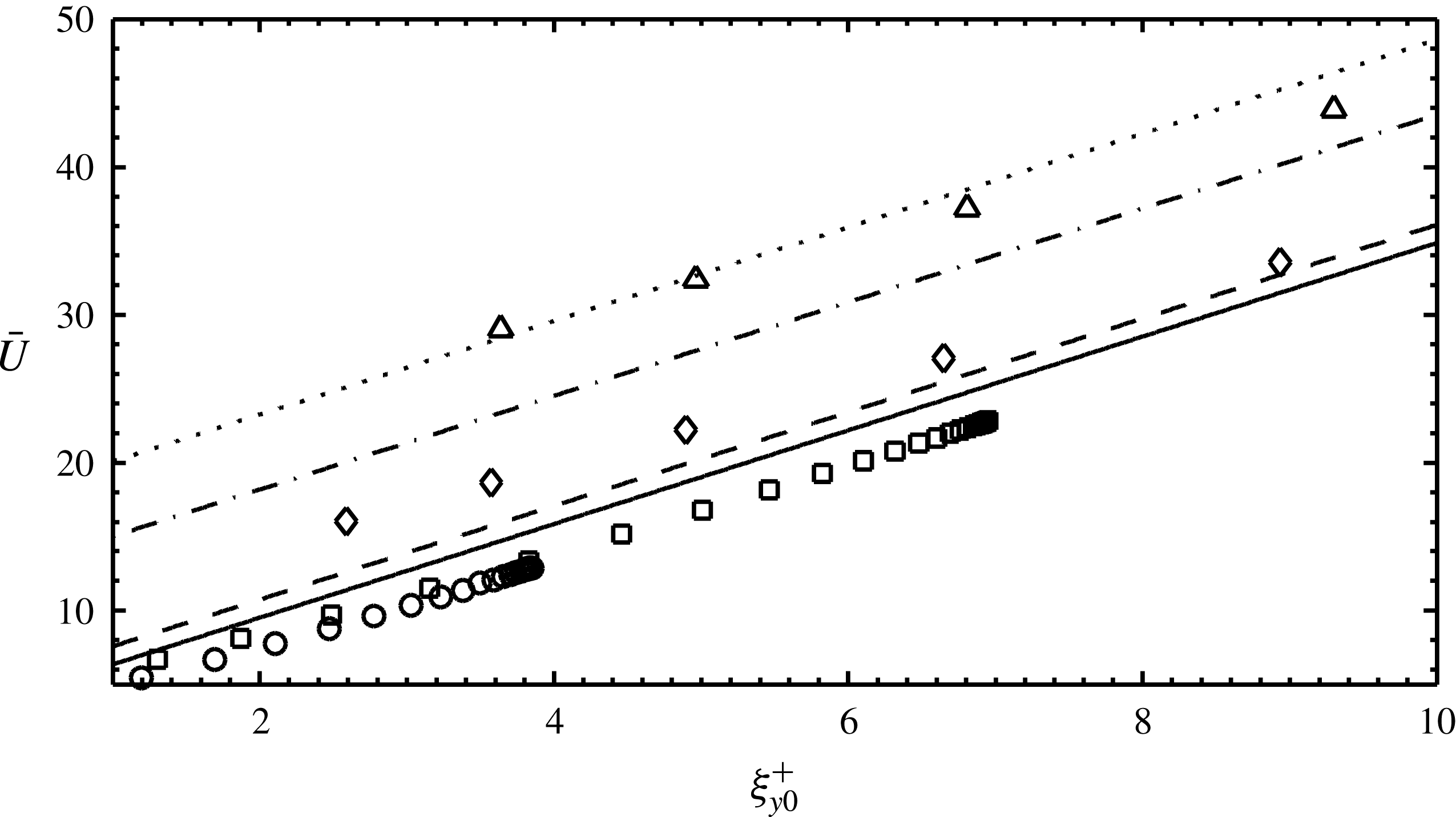
where $E\equiv [(A-D)/0.6]^{1/2}{\it\sigma}^{1/2}-18{\it\sigma}/(0.6\mathit{St})$ and we have neglected a term proportional to $[(A-D){\it\xi}_{y0}^{+}]^{2}$ . In this approximation, the depth-averaged fluid velocity is linearly related to the particle take-off velocity. The quantity $E$ can be interpreted as the excess in the depth-averaged horizontal fluid velocity over the mean of the horizontal particle velocities before and after the impact, which is needed to sustain the particle motion. Figure 4 shows that the uniform fluid velocity obtained from (3.9) is proportional to the horizontal fluid velocity, depth-averaged through the trajectory height, measured in the numerical solutions for the periodic trajectories. The latter have been obtained for different values of the Shields parameter, given the Stokes number and the density ratio. Hence, figure 4 also shows that the depth-averaged fluid velocity is independent of the strength of the fluid flow, a rather counterintuitive result.

Figure 4.

Horizontal fluid velocity, depth-averaged over the trajectory height, obtained from the numerical solutions for the periodic trajectories at large Stokes numbers versus take-off velocity. The symbols are the same as in figure 2. The lines are the analytical approximations (3.9) when $\mathit{St}=1000$ and ${\it\sigma}=5$ (solid), ${\it\sigma}=10$ (dashed), ${\it\sigma}=100$ (dot-dashed) and ${\it\sigma}=1000$ (dotted).

3.3. Trajectory length

Equation (3.8) then provides the particle horizontal velocity at every instant  $t$ . Upon integrating,

(3.10) $$\begin{eqnarray}\displaystyle x & = & \displaystyle \bar{U}t+\frac{{\it\sigma}}{0.3}\frac{18}{\mathit{St}}t-\frac{{\it\sigma}}{0.3}\ln \left[\exp \left(\frac{18}{\mathit{St}}t\right)-\frac{0.3\mathit{St}(\bar{U}-{\it\xi}_{x0}^{+})}{0.3\mathit{St}(\bar{U}-{\it\xi}_{x0}^{+})+18{\it\sigma}}\right]\nonumber\\ \displaystyle & & \displaystyle +\,\frac{{\it\sigma}}{0.3}\ln \left[1-\frac{0.3\mathit{St}(\bar{U}-{\it\xi}_{x0}^{+})}{0.3\mathit{St}(\bar{U}-{\it\xi}_{x0}^{+})+18{\it\sigma}}\right].\end{eqnarray}$$

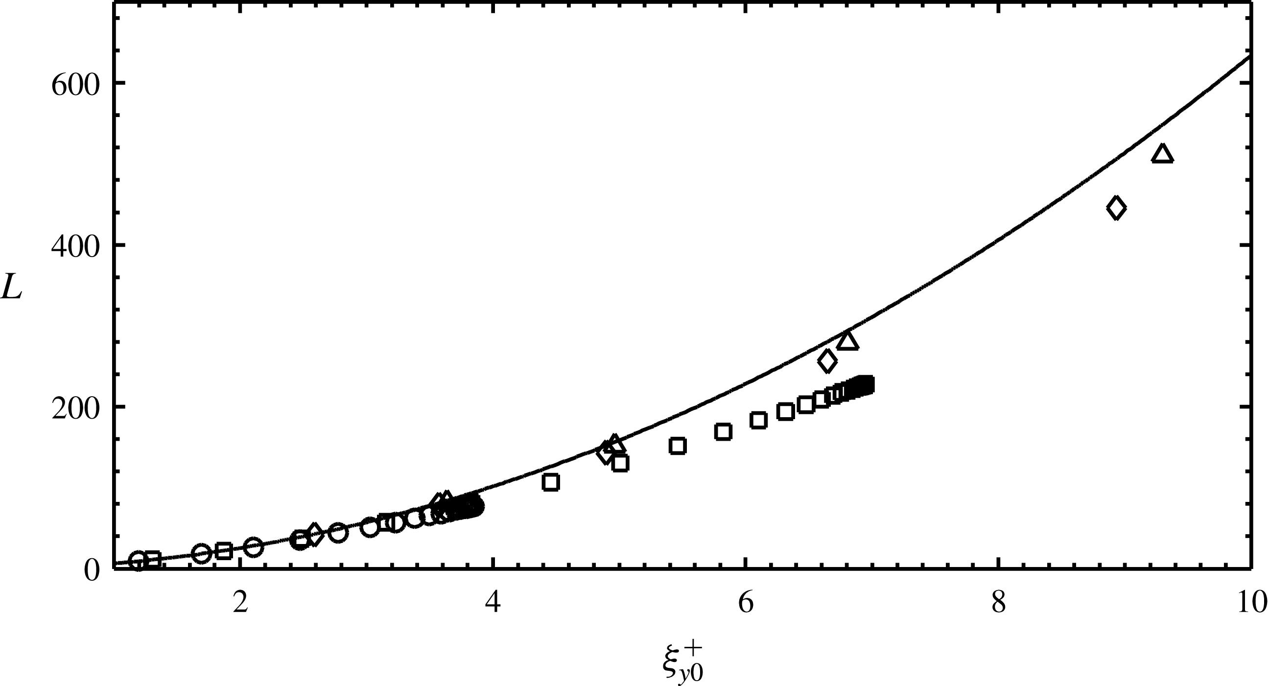
If we employ (3.9) in this and take $t=2{\it\xi}_{y0}^{+}$ , we can calculate the trajectory length. The result is well approximated by

(3.11) $$\begin{eqnarray}L\simeq (A+D){\it\xi}_{y0}^{+2},\end{eqnarray}$$

as demonstrated in figure 5.

Figure 5.

Trajectory length versus take-off velocity at large Stokes numbers. The symbols are the same as in figure 3. The solid line is the analytical approximation (3.11) to the trajectory length.

3.4. Fluid shear stress

If the horizontal fluid velocity follows the turbulent logarithmic profile based on the roughness, we can calculate the fluid shear stress at the bed, $S_{0}$ , as (appendix B)

(3.12) $$\begin{eqnarray}S_{0}=K\frac{{\it\kappa}^{2}}{{\it\sigma}[\ln (H/y_{0})]^{2}}\bar{U}^{2},\end{eqnarray}$$

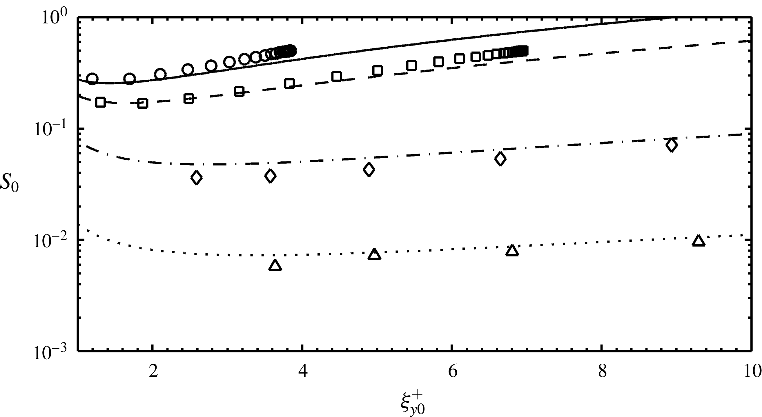
where $K$ is a coefficient of order one, which we determine on the basis of comparisons with the full numerical solution of the equations for the periodic trajectories. With $K=1.5$ , the agreement with the results of the numerical solution is good (figure 6). Once again, the fluid shear stress depends only on the take-off velocity and is independent of $S^{\ast }$ , so the numerical solutions to the periodic trajectories for different Shields parameters collapse onto a single curve.

Figure 6.

Fluid shear stress at the bed versus take-off velocity at large Stokes numbers. The symbols are the same as in figure 2. The lines are the analytical approximations to the fluid shear stress at the bed (3.12) with $K=1.5$ and $\mathit{St}=1000$ for ${\it\sigma}=5$ (solid), ${\it\sigma}=10$ (dashed line), ${\it\sigma}=100$ (dot-dashed line) and ${\it\sigma}=1000$ (dotted line).

For the fluid shear stress at the bed to be positive, the trajectory height must be greater than $y_{0}$ , so, from (3.1), ${\it\xi}_{y0}^{+}\geqslant (2y_{0})^{1/2}$ . In fact, for continuing saltation to exist, the height of the periodic trajectory should be greater than one diameter; so, in dimensionless terms, ${\it\xi}_{y0}^{+}\geqslant \sqrt{2}$ .

The minimum of the fluid shear stress in figure 6 corresponds to the smallest Shields parameter for which continuing saltation is possible over a rigid bumpy bed. The difference between the Shields parameter and the fluid shear stress at the bed is indeed the particle shear stress, which must be positive. Using (3.1), (3.3), (3.6) and (3.9) in (3.12), and requiring that the derivative with respect to the take-off velocity be zero, permits the determination of the take-off velocity at the minimum. Its approximate expression is

(3.13) $$\begin{eqnarray}{\it\xi}_{y0}^{+c}=\max \left\{\exp \left[1+\frac{1}{2}\frac{(A+D)\ln (2y_{0})}{A+D+2E}\right],\sqrt{2}\right\},\end{eqnarray}$$

where we have assumed that $\ln {\it\xi}_{y0,c}^{+}\simeq 1-1/{\it\xi}_{y0,c}^{+}$ . This value, used in (3.12), gives the critical Shields parameter $S_{c}^{\ast }$ at which continuing saltation ceases:

(3.14) $$\begin{eqnarray}S_{c}^{\ast }=\frac{K{\it\kappa}^{2}}{{\it\sigma}[2\ln {\it\xi}_{y0}^{+c}-\ln (2y_{0})]^{2}}\left(\frac{A+D}{2}{\it\xi}_{y0}^{+c}+E\right)^{2}.\end{eqnarray}$$

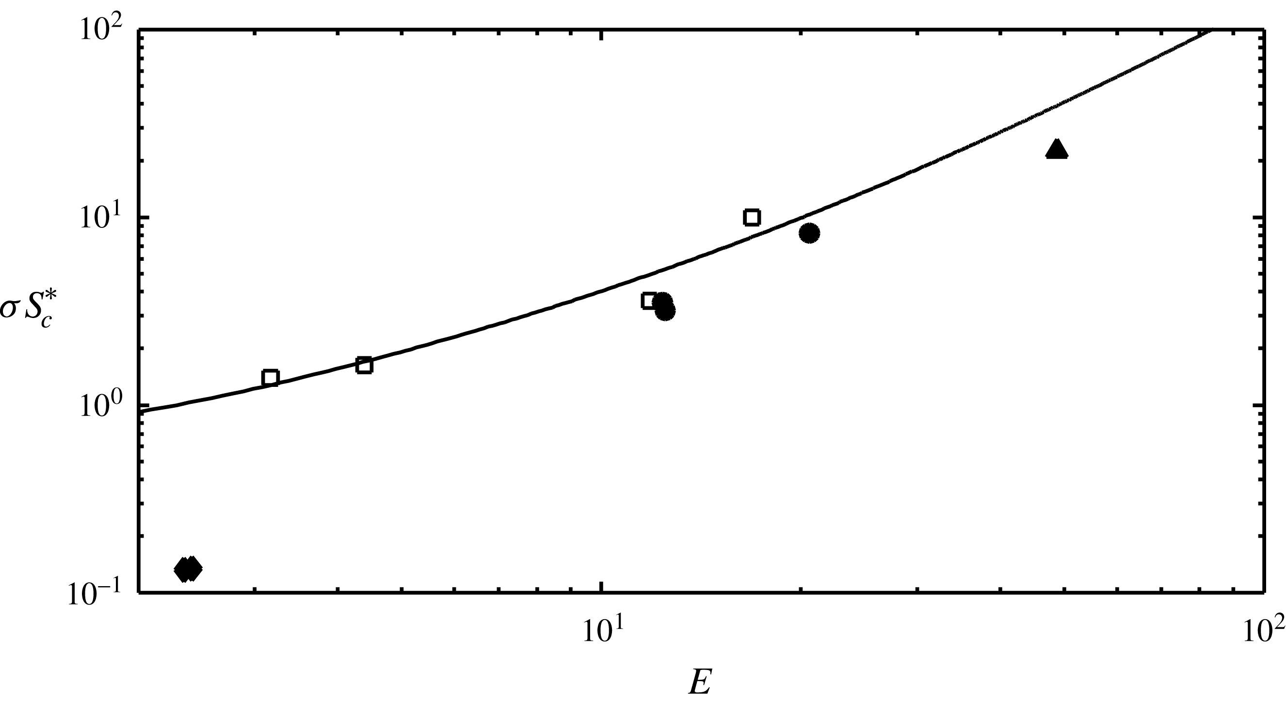
Equations (3.13) and (3.14) indicate that the product of this critical Shields number and the density ratio is a function only of  $E$ . We anticipate that (3.13) and (3.14) are valid also for continuing saltation over erodible beds. There is only a small quantitative difference between the rigid and the erodible beds, due to the different values of the numerical coefficients $a$ , $b$ , $a_{y}$ and $b_{y}$ in the rebound relations, which determine the values of $A$ and $D$ . Figure 7 shows the comparison between values of this product obtained numerically and analytically versus  $E$ . Also shown are the values of the product for the initiation of particle motion over erodible beds obtained in experiments: ${\it\sigma}=2.5$ and $\mathit{St}$ between 1000 and 32 000 (Meyer-Peter & Müller Reference Meyer-Peter and Müller1948), ${\it\sigma}=2500$ and $\mathit{St}=3000$ (Creyssels et al. Reference Creyssels, Dupont, Ould El Moctar, Valance, Cantat, Jenkins, Pasini and Rasmussen2009), and ${\it\sigma}$ between 80 and 200 and $\mathit{St}$ between 4000 and 8500 (Burr et al. Reference Burr, Bridges, Marshall, Smith, White and Emery2015). Only data for hydrodynamically rough beds have been taken from the experiments. The predicted values of $S_{c}^{\ast }$ for density ratios larger than 50 are close to the values of the minimum Shields number for particle motion, indicating that there is a transition from no motion to continuing saltation. In contrast, the aquatic data of Meyer-Peter & Müller (Reference Meyer-Peter and Müller1948), for which the Shields parameter is less than $S_{c}^{\ast }$ , indicate that there the motion is not characterized by continuing saltation. In other words, the mean motion of the fluid is not enough to sustain the particle transport. Indeed, in that case, turbulence bursts are responsible for the particle motion, which is characterized by intermittency (Ancey et al. Reference Ancey, Davison, Böhm, Jodeau and Frey2008; Radice et al. Reference Radice, Ballio and Nikora2009; Singh et al. Reference Singh, Fienberg, Jerolmack, Marr and Foufoula-Georgiou2009; Lajeunesse et al. Reference Lajeunesse, Malverti and Charru2010).

Figure 7.

Product of the critical Shields parameter and the density ratio for continuing saltation versus the quantity  $E$ , as obtained from the analytical approximation (3.14) (line) and the numerical integrations for the periodic trajectories at large Stokes numbers (hollow squares). Also shown are the experimental values (solid symbols) of the product of the minimum Shields number and the density ratio for the initiation of steady particle motion obtained by Meyer-Peter & Müller (Reference Meyer-Peter and Müller1948, diamonds), Creyssels et al. (Reference Creyssels, Dupont, Ould El Moctar, Valance, Cantat, Jenkins, Pasini and Rasmussen2009, triangles) and Burr et al. (Reference Burr, Bridges, Marshall, Smith, White and Emery2015, circles).

3.5. Horizontal particle flux

Given the Shields parameter $S^{\ast }$ , the particle shear stress at the bed is

(3.15) $$\begin{eqnarray}s_{0}=S^{\ast }-K\frac{{\it\kappa}^{2}}{{\it\sigma}[\ln (H/y_{0})]^{2}}\bar{U}^{2}.\end{eqnarray}$$

Unlike the fluid shear stress, the particle shear stress at the bed is influenced by the Shields parameter. Then, from (2.9), (2.10) and (3.2),

(3.16) $$\begin{eqnarray}c_{0}^{+}=\frac{s_{0}}{{\it\xi}_{y0}^{+}({\it\xi}_{x0}^{-}-{\it\xi}_{x0}^{+})}.\end{eqnarray}$$

Equations (3.15) and (3.16) relate the take-off velocity, the concentration and the Shields parameter or, alternatively, the depth-averaged fluid velocity, the concentration and the Shields parameter. The horizontal particle flux per unit width of the bed can then be calculated as

(3.17) $$\begin{eqnarray}Q=c_{0}^{+}L{\it\xi}_{y0}^{+}.\end{eqnarray}$$

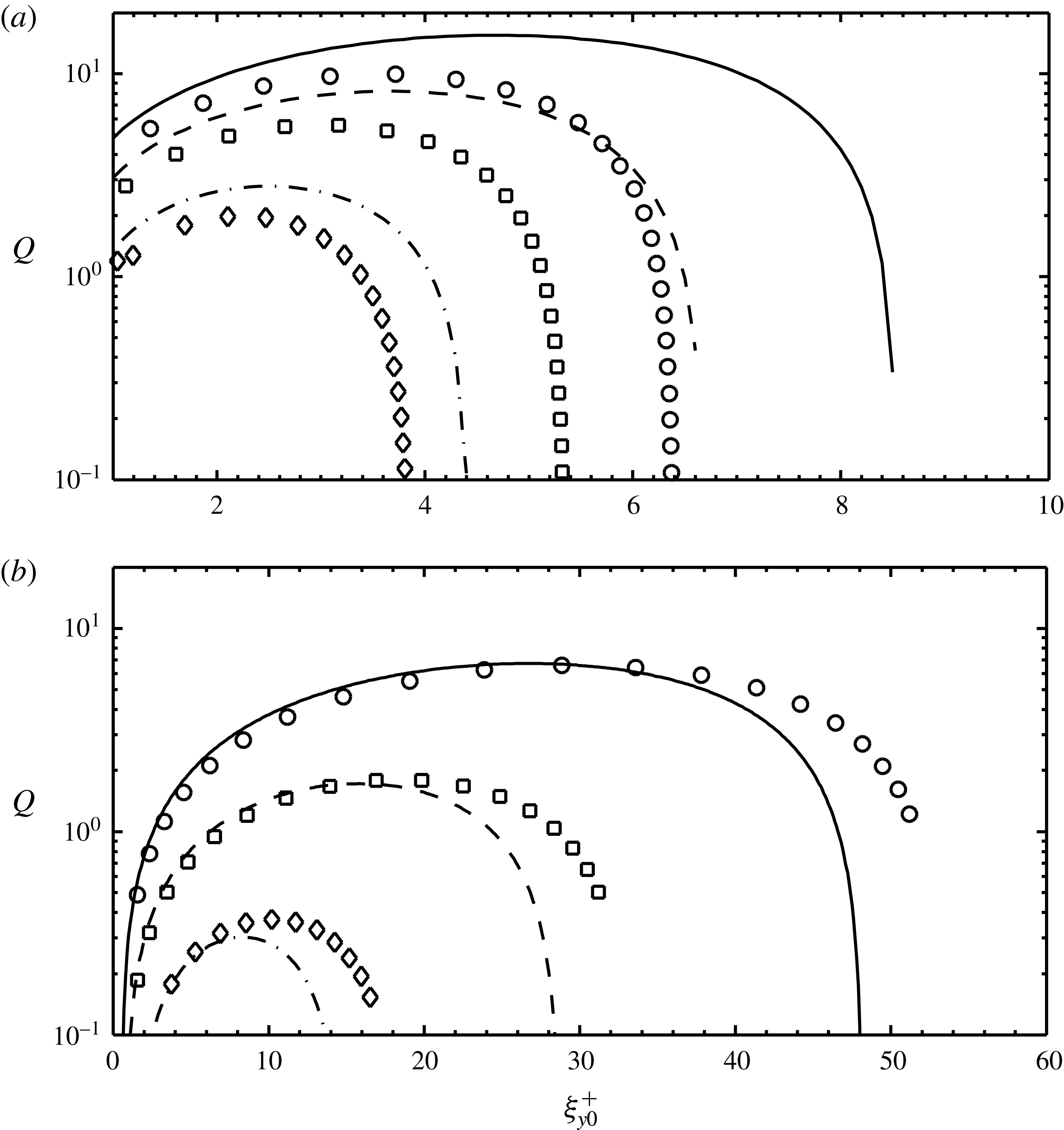
Figure 8(a,b) shows the comparison between the horizontal particle flux evaluated from the full numerical integration of the equations for the periodic trajectories at large Stokes numbers and that obtained from the approximate analytical approach for two extreme values of the density ratio at different Shields parameters, with the flux linearly increasing with the Shields parameter.

Figure 8.

Horizontal particle flux versus take-off velocity for periodic saltation over rigid beds when $\mathit{St}=1000$ : (a)  ${\it\sigma}=5$ and $S^{\ast }=0.3$ (triangles and dotted line), 0.5 (diamonds and dot-dashed line), 0.8 (squares and dashed line), 1.1 (circles and solid line); and (b)  ${\it\sigma}=1000$ and $S^{\ast }=0.02$ (diamonds and dot-dashed line), 0.04 (squares and dashed line) and 0.08 (circles and solid line). The symbols are the numerical solutions for the periodic trajectories and the lines are the analytical approximation to the particle flux (3.17).

As already noticed in the experiments of Ho et al. (Reference Ho, Valance, Dupont and Ould El Moctar2011) and in the analysis of Jenkins & Valance (Reference Jenkins and Valance2014) on aeolian transport over rigid beds, there is a maximum horizontal particle flux $Q_{\mathit{max}}$ that the fluid can sustain at a given Shields parameter: the maximum transport capacity of the flow. Our analysis suggests that this observation holds irrespective of the density ratio. We can determine the value of the take-off velocity, $\hat{{\it\xi}}_{y0}^{+}$ , that corresponds to $Q_{\mathit{max}}$ by requiring the derivative of (3.17) with respect to ${\it\xi}_{y0}^{+}$ to be zero, using (3.1), (3.3), (3.6), (3.9), (3.11), (3.15) and (3.16). This results in the condition

(3.18) $$\begin{eqnarray}\displaystyle \frac{{\it\sigma}S^{\ast }}{K{\it\kappa}^{2}} & = & \displaystyle \left[\left(\frac{A+D}{2}\hat{{\it\xi}}_{y0}^{+}+E\right)(A+D)\hat{{\it\xi}}_{y0}^{+}+\left(\frac{A+D}{2}\hat{{\it\xi}}_{y0}^{+}+E\right)^{2}\right]\left[\ln \left(\frac{\hat{{\it\xi}}_{y0}^{+2}}{2y_{0}}\right)\right]^{-2}\nonumber\\ \displaystyle & & \displaystyle -\,4\left(\frac{A+D}{2}\hat{{\it\xi}}_{y0}^{+}+E\right)^{2}\left[\ln \left(\frac{\hat{{\it\xi}}_{y0}^{+2}}{2y_{0}}\right)\right]^{-3}.\end{eqnarray}$$

With this and (3.9), (3.11), (3.15), (3.16) and (3.17), the maximum transport capacity $Q_{\mathit{max}}$ can then be calculated as

(3.19) $$\begin{eqnarray}{\it\sigma}Q_{\mathit{max}}=\frac{A+D}{A-D}\left[{\it\sigma}S^{\ast }-K\frac{{\it\kappa}^{2}}{[2\ln \hat{{\it\xi}}_{y0}^{+}-\ln (2y_{0})]^{2}}\left(\frac{A+D}{2}\hat{{\it\xi}}_{y0}^{+}+E\right)^{2}\right]\hat{{\it\xi}}_{y0}^{+}.\end{eqnarray}$$

Equation (3.19) provides a relation between $Q_{\mathit{max}}$ , $S^{\ast }$ and ${\it\sigma}$ , once $\hat{{\it\xi}}_{y0}^{+}$ is determined as a function of $S^{\ast }$ from (3.18). With $\hat{{\it\xi}}_{y0}^{+}$ , all the quantities that characterize the periodic trajectory at the maximum transport capacity can easily be obtained from the equations introduced in this section.

4. Approximate analytical solution: periodic saltation over an erodible bed

In continuing steady saltation over erodible beds, there is, in principle, an unlimited supply of material that can be incorporated in the flow. The horizontal particle flux may be calculated for all impact velocities. If the flux corresponding to half the critical impact velocity resides to the right of the maximum, an increment of impact velocity to its left results in an increase in flux, and erosion from the bed. With continued migration of the impact velocity to the left, the increase in horizontal particle flux and erosion continues until the maximum horizontal flux is achieved. The horizontal particle flux $Q$ is always equal to $Q_{\mathit{max}}$ of (3.19), with $\hat{{\it\xi}}_{y0}^{+}$ calculated from (3.18), when it is less than ${\it\xi}_{c}/(2B)$ , and equal to ${\it\xi}_{c}/(2B)$ otherwise. We refer to these cases as unlimited and splash-limited saltation, respectively. The condition $\hat{{\it\xi}}_{y0}^{+}={\it\xi}_{c}/(2B)$ is the constraint assumed by Jenkins & Valance (Reference Jenkins and Valance2014) in their analysis of aeolian transport over erodible beds. Aeolian transport over an erodible bed is splash-limited, while aquatic transport is not.

The boundary between unlimited and splash-limited saltation is, from (3.18) with $\hat{{\it\xi}}_{y0}^{+}={\it\xi}_{c}/(2B)$ , at the Shields parameter

(4.1) $$\begin{eqnarray}\displaystyle \frac{{\it\sigma}S_{s}^{\ast }}{K{\it\kappa}^{2}} & = & \displaystyle \left[\left(\frac{A+D}{2}\frac{{\it\xi}_{c}}{2B}+E\right)(A+D)\frac{{\it\xi}_{c}}{2B}+\left(\frac{A+D}{2}\frac{{\it\xi}_{c}}{2B}+E\right)^{2}\right]\left[\ln \left(\frac{{\it\xi}_{c}^{2}}{8B^{2}y_{0}}\right)\right]^{-2}\nonumber\\ \displaystyle & & \displaystyle -\,4\left(\frac{A+D}{2}\frac{{\it\xi}_{c}}{2B}+E\right)^{2}\left[\ln \left(\frac{{\it\xi}_{c}^{2}}{8B^{2}y_{0}}\right)\right]^{-3}.\end{eqnarray}$$

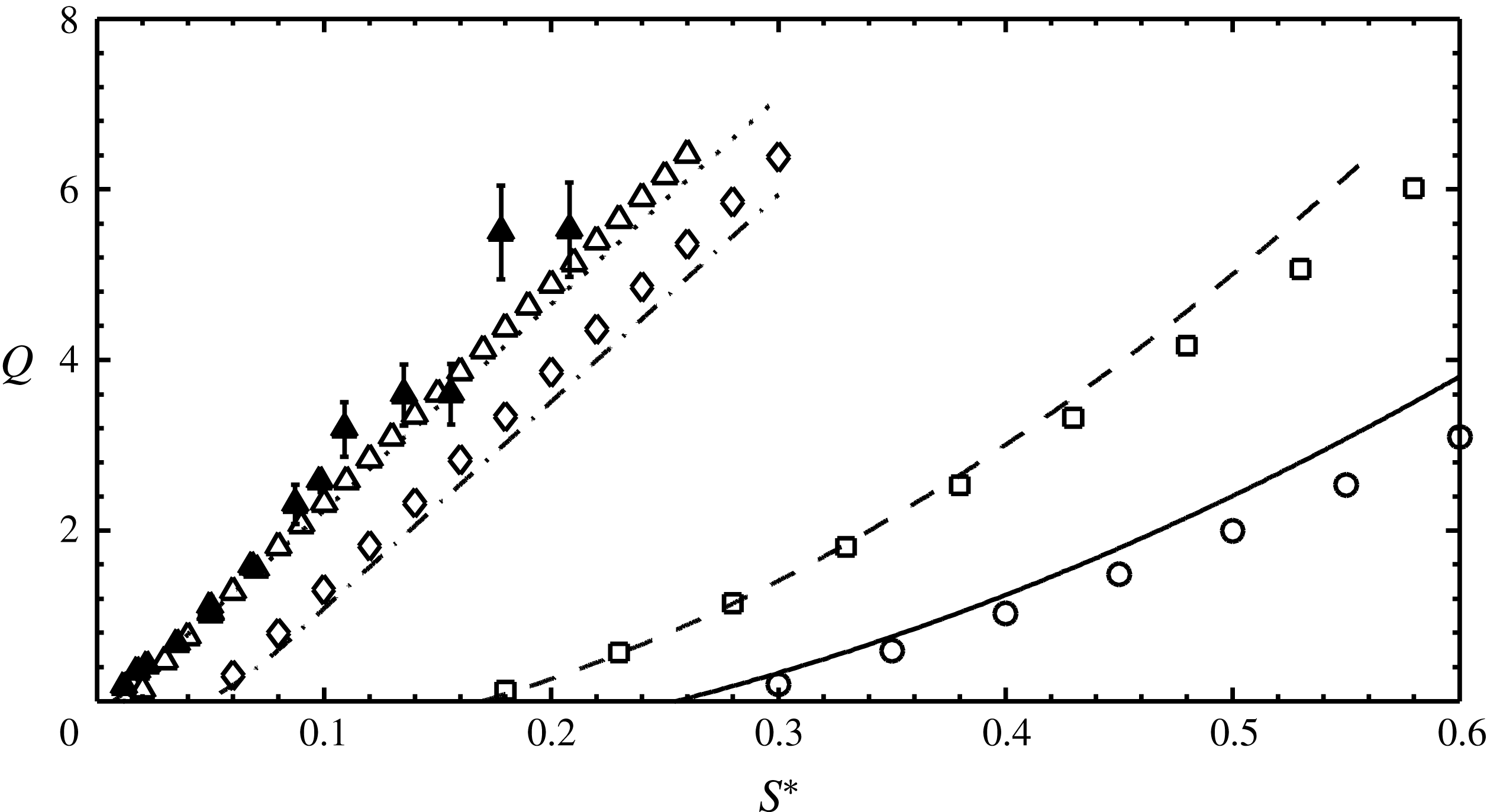
Unlimited saltation takes place for Shields parameters in the range from $S_{c}^{\ast }$ to $S_{s}^{\ast }$ ; splash-limited saltation occurs for Shields parameters larger than $S_{s}^{\ast }$ . As demonstrated in Jenkins & Valance (Reference Jenkins and Valance2014), the two regimes are characterized by different scalings of the various quantities with the Shields parameter. In particular, the horizontal particle flux scales with the $3/2$ power of the difference between the Shields parameter and $S_{c}^{\ast }$ in unlimited saltation (it is the scaling of the maximum transport capacity over rigid beds); while it scales linearly with the Shields parameter in the splash-limited case. Figure 9 shows the comparison between the analytical horizontal particle flux as a function of the Shields parameter for periodic saltation over erodible beds and the results of the numerical solutions for the periodic trajectories for large Stokes numbers. To determine the latter, we use the same criterion as in the analytical solution: the particle flux at a given Shields parameter is the maximum in the curves of figure 8 – calculated through interpolation – unless the corresponding impact velocity exceeds ${\it\xi}_{c}/2$ . In the latter case, we take the horizontal particle flux to be the value to the left of the maximum at which the impact velocity is exactly ${\it\xi}_{c}/2$ . Also shown in figure 9 are the experimental values obtained by Creyssels et al. (Reference Creyssels, Dupont, Ould El Moctar, Valance, Cantat, Jenkins, Pasini and Rasmussen2009) and Ho et al. (Reference Ho, Valance, Dupont and Ould El Moctar2011) for sand in air. The analytical solution for ${\it\sigma}=2500$ and $\mathit{St}=3000$ , as in the experiments, is indistinguishable from that for ${\it\sigma}=1000$ and $\mathit{St}=1000$ . As in the numerical simulations of Durán et al. (Reference Durán, Andreotti and Claudin2012), the horizontal particle flux scales linearly with the Shields parameter in the aeolian case ( ${\it\sigma}=1000$ ) – splash-limited saltation – and is roughly proportional to the Shields parameter to the power of $3/2$ in the nearly aquatic case ( ${\it\sigma}=5$ ) – unlimited saltation. Intermediate values of the density ratio ( ${\it\sigma}=100$ ) are characterized by a mixed behaviour: the flux follows the unlimited saltation scaling close to the threshold, and the splash-limited saltation scaling for larger values of the Shields parameter. Our interpretation for the linear relationship between the horizontal particle flux and the Shields parameter in aeolian saltation over erodible beds is based on the same argument as Durán et al. (Reference Durán, Andreotti and Claudin2012): the splash process is the key mechanism that controls the saltation. The only difference is that we take the particle horizontal velocity proportional to the critical impact velocity, whereas Durán et al. suggest that it scales with the fluid horizontal velocity at the transport threshold.

Figure 9.

Horizontal particle flux versus Shields parameter for saltation over erodible beds for $\mathit{St}=1000$ , when ${\it\sigma}=5$ (circles and solid line), ${\it\sigma}=10$ (squares and dashed line), ${\it\sigma}=100$ (diamonds and dot-dashed line) and ${\it\sigma}=1000$ (triangles and dotted line). The hollow symbols are the numerical solutions for the periodic trajectories and the lines are the analytical approximation to the particle flux (3.19). Also shown are the experimental results of Creyssels et al. (Reference Creyssels, Dupont, Ould El Moctar, Valance, Cantat, Jenkins, Pasini and Rasmussen2009) and Ho et al. (Reference Ho, Valance, Dupont and Ould El Moctar2011) (solid triangles) with the relative error bars.

Saltation alone takes place when inter-particle collisions above the bed are not likely. This is no longer true when twice the height of the trajectory $H$ is greater than the mean free path of kinetic theory, $\sqrt{2}/12c_{0}$ (Chapman & Cowling Reference Chapman and Cowling1970; Pasini & Jenkins Reference Pasini and Jenkins2005), where $c_{0}=c_{0}^{+}+c_{0}^{-}$ . The height of the trajectory and the concentration at the bed can be calculated from the relations derived in the previous section, with the take-off velocity equal to the minimum between $\hat{{\it\xi}}_{y0}^{+}$ , calculated from (3.18), and ${\it\xi}_{c}/(2B)$ . 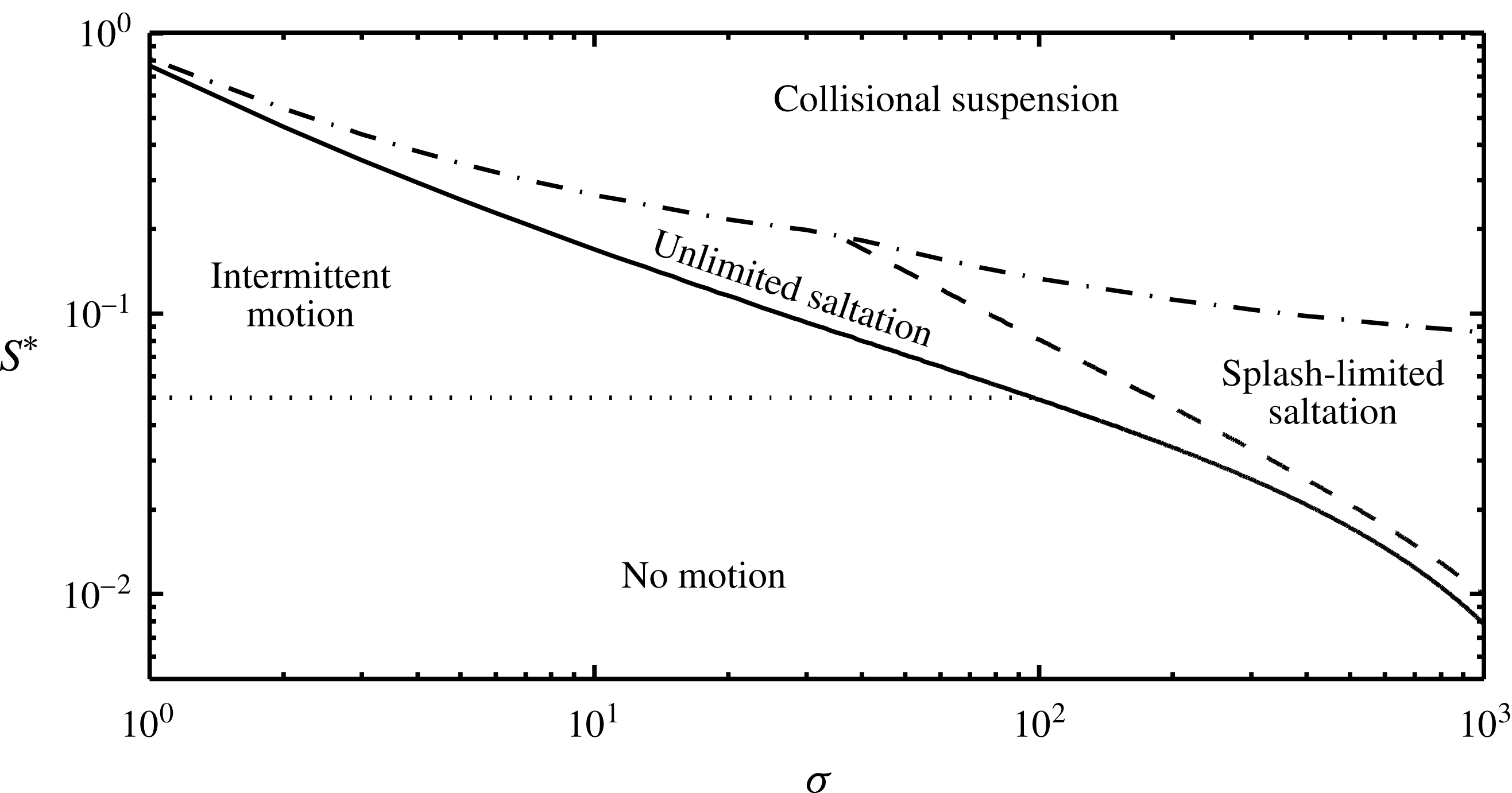This provides an upper limit for the existence of a pure saltation regime in terms of the Shields parameter as a function of the density ratio at a given Stokes number. Above this limit, collisional suspension begins to take place (Jenkins & Hanes Reference Jenkins and Hanes1998; Pasini & Jenkins Reference Pasini and Jenkins2005; Berzi Reference Berzi2013).

Figure 10 shows a regime map in terms of Shields parameter versus density ratio for a Stokes number of 1000. At large density ratios (aeolian transport), there is a rather abrupt transition from no motion to continuing saltation, and the latter is essentially limited by the splash. Also the range of Shields parameter in which continuing saltation exists is significant. This confirms that saltation is the main mode of transport for sand in air. On the other hand, at small density ratios (aquatic transport), the intermittent motion is dominant up to large Shields parameters, at which there is a rather abrupt transition to collisional suspension. In this case, continuing saltation, not limited by the splash, is only marginally relevant. Intermediate values of the density ratio, typical of many extraterrestrial environments, are more complicated: intermittent motion, unlimited and splash-limited saltation and collisional suspension seem to play equally significant roles in the transport of sediments.

Figure 10.

Regime map for $\mathit{St}=1000$ . The boundary between the regimes of intermittent motion and no motion is qualitatively determined (Durán et al. Reference Durán, Andreotti and Claudin2012).