


1. Introduction
Climate change poses the greatest long-run challenge for humanity: the poorest of the poor will suffer most yet have contributed least to the problem and the richest of the rich may even benefit despite being major contributors. Over deep time, climate change has caused all the great extinctions, obviously not from anthropogenic greenhouse gas (GHG) emissions, but we are now the main threat due to burning fossil fuels, construction and modern agriculture and may become one of the victims from feedback loops.
Tipping points include tundra melting releasing large amounts of methane, rapidly raising atmospheric temperatures, feeding onto ocean heat and starting to melt methane hydrates, which store more than all other fossil fuels combined. Already we are observing a less stable jet stream as Arctic amplification reduces the temperature contrast between the Arctic and lower latitudes. More persistent atmospheric circulation patterns can contribute to prolonged weather patterns, driving extreme heat and marine heat waves, and leading to hotter summers and colder winters. The impacts include increasing wildfires, ‘rivers in the sky’ leading to ever worsening floods, yet also potentially greater and longer droughts, where the interrelationship between extreme rainfall phases followed by drought exacerbates wildfires. We are also observing more violent cyclones, polar ice melting affecting ocean circulation with rising sea levels, and greater mismatches in plants and insects for breeding times by animals and birds. The combination of high temperature and humidity due to climate change is raising wet bulb heat, which is dangerous to life.
Yet, by 1900, everything needed to avoid a climate crisis was known: continuous batteries; electromagnetic and hydro generators; constant-speed electric motors with regenerative braking; electrolysis; fuel cells; photovoltaic solar cells; reversible heat pumps; wind turbines; rechargeable batteries; and direct current (DC) to alternating current (AC). These led to dozens of other invaluable inventions like refrigeration, telegraph, telephone, light bulbs and so forth. Many of these inventions were developed in Britain, but it was the US which predominantly converted such ideas into mass market products. The dominance of coal in the UK may well have suppressed competition for electric products. Moreover, it was known that carbon dioxide was a GHG. As we discuss, a low fossil fuel world was within humanity’s grasp—but free markets, which take no account of externalities or the curse of the commons, chose the fossil fuel route.Footnote 1
We set the scene in Section 2 by looking at UK energy consumption data over the very long run, before exploring the knowledge that was established in the 19th century in Section 3. Section 4 looks at the implications that followed from pursuing the fossil fuel path, and draws lessons for policy-makers, before Section 5 models and forecasts the UK energy mix, resulting in a 24-year ahead forecast which is then used to produce a scenario projection of the all-electric energy path in 1900. Section 6 concludes.
2. Energy consumption
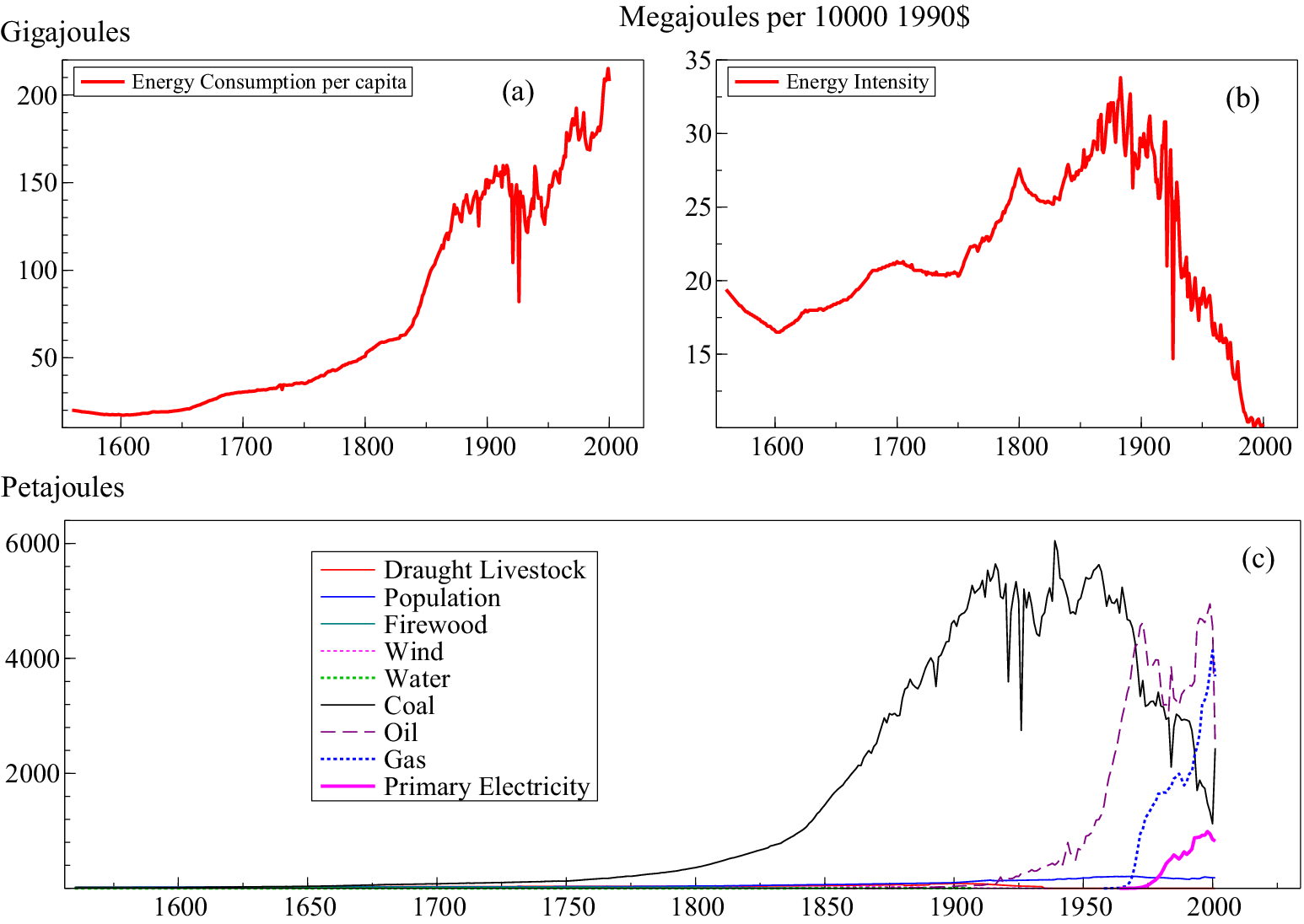
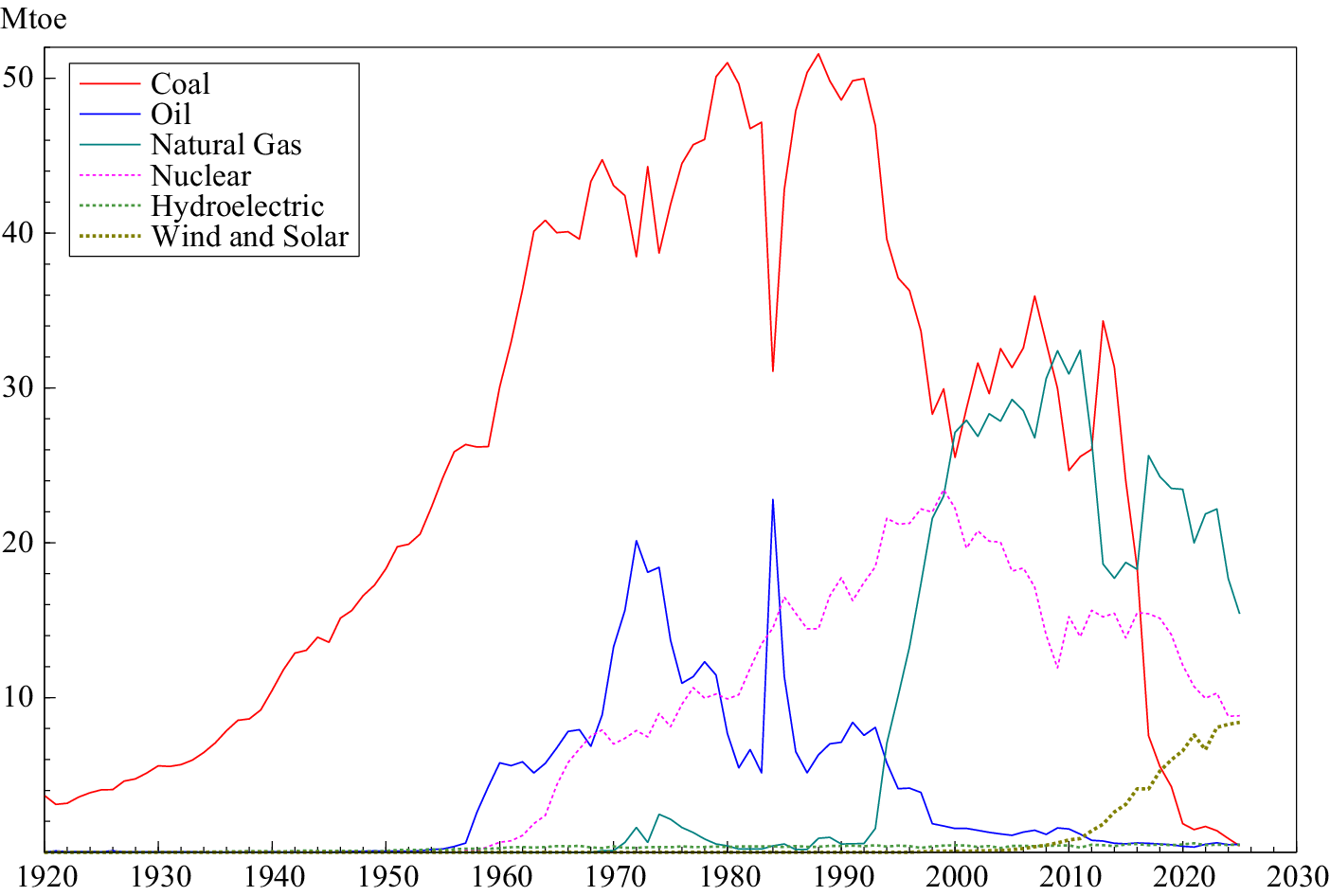
Warde (Reference Warde2007) produces data on energy consumption and energy intensity for the UK from 1560 to 2000, recorded in Figure 1. Coal was the dominant source by the mid-18th century, and accelerated due to the expansion of the railways, seen in panel (c). Coal accounted for around 95% of all energy consumption in Britain by the beginning of the 20th century and it remained dominant until post-WWII when oil, followed by natural gas, was established, and only recently have we seen electricity increase rapidly, initially due to nuclear but now driven by renewables. Figure 2 records the breakdown of fuel input for electricity generation from 1920 onwards, in which all fossil fuels are declining and renewables are accelerating since the 2000s. Thus, we are witnessing the transition from a fossil fuel economy to an all-electric world, but many of the costs of burning fossil fuels are baked in. Hence, it is worth considering what an all-electric world would have looked like over a century ago, and whether there are lessons from this alternative universe that can help with the net-zero transition.
(a) UK energy consumption per capita from 1560 to 2000; (b) energy intensity, measured as the energy it takes to produce a unit of income; (c) composition of energy consumption including food, firewood, fodder for working animals, wind, water, coal, oil, natural gas and primary electricity.

Figure 1. Long description
The figure contains three panels labeled a, b, and c.
Panel a is a line graph of Energy Consumption per capita. The x-axis represents years from 1560 to 2000. The y-axis represents Gigajoules from 0 to 200. The red line shows a slow, steady increase from 1560 to 1800, followed by a sharp exponential rise. There is a significant dip around 1920 before continuing to a peak of over 200 Gigajoules by 2000.
Panel b is a line graph of Energy Intensity. The x-axis represents years from 1560 to 2000. The y-axis represents Megajoules per 10000 1990 dollars, ranging from 10 to 35. The red line fluctuates between 15 and 20 until 1650, rises to a peak of 34 around 1880, and then shows a steep, volatile decline toward 10 by the year 2000.
Panel c is a line graph showing the composition of energy consumption. The x-axis represents years from 1560 to 2000. The y-axis represents Petajoules from 0 to 6000.
- Draught Livestock, Population, Firewood, Wind, and Water remain near the baseline throughout the period.
- Coal (black line) begins a rapid ascent around 1800, peaking near 6000 Petajoules in the early 1900s before declining sharply after 1950.
- Oil (purple dashed line) rises sharply starting around 1950, peaking near 5000 Petajoules around 1970.
- Gas (blue dotted line) and Primary Electricity (pink line) show significant increases starting after 1970.
Breakdown of fuel inputs for UK electricity generation in Mtoe, on an energy supplied basis.

Figure 2. Long description
The x-axis represents years from 1920 to 2030 in 10-year increments. The y-axis represents energy in M toe from 0 to 50.
* Coal (solid red line): Shows a steady linear increase from approximately 5 M toe in 1920 to a peak of over 50 M toe in the late 1980s. It then experiences a sharp, rapid decline after 2010, reaching near zero by 2025.
* Oil (solid blue line): Remains near zero until the 1950s, peaks at 20 M toe in the early 1970s, drops sharply, has a brief spike in the mid-1980s, and then declines to near zero.
* Natural Gas (solid teal line): Remains at zero until the early 1990s, where it shows a rapid vertical increase, peaking at over 30 M toe around 2010 before trending downward to 15 M toe by 2025.
* Nuclear (pink dashed line): Begins in the late 1950s, showing a steady increase to a peak of 23 M toe around 2000, followed by a gradual decline to approximately 8 M toe by 2025.
* Hydroelectric (green dotted line): Maintains a constant, near-zero horizontal line across the entire period.
* Wind and Solar (brown dotted line): Remains at zero until approximately 2010, then shows a steady linear increase to nearly 10 M toe by 2025.
3. Historical knowledge and understanding
We explore the 19th-century understanding of electricity generation in Section 3.1, the uses of electricity that were developed in Section 3.2 and the knowledge of GHGs in Section 3.3.
3.1. Generating electricity in the 19th century
There were many investigators of electricity before Alessandro Volta created his ‘voltaic pile’ in 1800. Of note, in the 1750s, Benjamin Franklin had conducted many experiments with electricity, of which the most famous were with lightning, leading to the life-saving development of a sharp, pointed and grounded lightning rod to prevent buildings being destroyed. Luigi Galvani in 1780 experimented with animal electricity, later reinterpreted by Alessandro Volta as due to Galvani’s use of a metal cable, leading to Volta’s ‘pile battery’, the first battery to generate a continuous flow of electricity (see Cecchini and Pelosi, Reference Cecchini and Pelosi1992). This development was immediately put to good use by William Nicholson and Anthony Carlisle discovering electrolysis, which surprisingly splits water into oxygen (air) and hydrogen (fire), shown by separately collecting these gases. In 1820, Hans Christian Ørsted discovered electromagnetism, followed a year later by Michael Faraday, with Humphry Davy and William Wollaston creating electromagnetic rotation. Within a decade, Faraday had invented the electric generator, the foundation of modern electricity production. This idea may have benefited from the development of a high-efficiency water turbine in 1826 by Benoit Fourneyron (see Smith, Reference Smith1980), also leading to the ‘Francis turbine’ in 1849 by James Francis and Uriah Boyden. Thus, by the early 1830s, electricity could be generated as needed, and stored in batteries.
Alternative methods for generating electricity soon followed. In 1838 Sir William Grove invented the fuel cell and the following year Edmond Becquerel (Reference Becquerel1839) created the photovoltaic cell, the basis for Charles Fritts (Reference Fritts1883) commercial photovoltaic solar panel (see Appleby, Reference Appleby1990). The first continuous UK electricity supply generated by hydroelectricity was in 1868 by Sir William Armstrong, although it took until 1880 for the first commercial hydroelectricity to be produced at Grand Rapids in Michigan (see Higgins, Reference Higgins2007). In 1887 James Blyth (Reference Blyth1894) developed a wind turbine to generate electricity, probably building on the functioning of centuries-old windmills combined with Faraday’s electric generator. Blyth’s development was adopted rapidly; for example, Fridtjof Nansen’s ship ‘Fram’ explored the Arctic over 1893–1896 with a windmill on board to generate electricity for lighting inside his ship during long dark winters.
3.2. 19th-century uses of electricity
The 19th century also saw many applications of electricity to practical and indeed often invaluable uses. In 1834 a refrigerator powered by electricity was patented by Jacob Perkins, although artificial refrigeration had first been demonstrated in 1748 by William Cullen long before electricity could make it ubiquitous. William Cooke and Charles Wheatstone developed the electric telegraph in 1837, which enabled instantaneous communication over long distances, followed by Alexander Graham Bell’s 1876 telephone. In between, the theory of heat pumps was established by Lord Kelvin in 1852, apparently countering the second law of thermodynamics by transferring heat from a cold to a hot body, with the first operational heat pump by Peter von Rittinger working in Switzerland by 1857. Incandescent light bulbs for efficient lighting were produced by Joseph Swan and Thomas Edison during the 1880s. A key practical advance for electricity transmission was the conversion of DC electricity to AC by Nikola Tesla in 1888, involving a long battle with Thomas Edison’s preference for DC (see Roguin, Reference Roguin2004). That year also saw the first electric street railway in Richmond, Va., developed by Frank Sprague, with a constant-speed motor and regenerative braking powered from overhead wires (see Jackson, Reference Jackson1943). During the 1880s, an electric car with a high-capacity rechargeable battery was produced by Thomas Parker.
3.3. Discovering greenhouse gases
Although not part of the history of electricity, showing that carbon dioxide (CO2) was a GHG and was given off by burning hydrocarbons was an important step in understanding climate change. In 1856, Eunice Foote (Reference Foote1856) had demonstrated that a flask of CO2 heated greatly in the sun, whereas a flask of dry air did not. John Tyndall (Reference Tyndall1860) who conducted experiments independently confirmed her results, and Svante Arrhenius (Reference Arrhenius1896) later proved that atmospheric temperature change was proportional to the change in log(CO2). On 14 August 1912, an article published in the Rodney and Otamatea Times, Waitemata and Kaipara Gazette stated that ‘The furnaces of the world are now burning about 2,000,000,000 tons of coal a year. When this is burned, uniting with oxygen, it adds about 7,000,000,000 tons of carbon dioxide to the atmosphere yearly. This tends to make the air a more effective blanket for the earth and to raise its temperature. The effect may be considerable in a few centuries’. Although the timing of the impacts was considerably optimistic, the causal link was explicitly known. Thus, the potential for burning fossil fuels to cause climate change was well-established at the start of the 20th century.
4. Implications
By 1900, electricity was well understood, as was how to generate it by hydro, solar and wind, convert it between DC and AC, store it, how to move people in cars and trams, and apply electricity in numerous applications still in use today for lighting, heating and cooling, as well as to communicate. It was also known that burning fossil fuels caused climate change. Thus, humanity was very close to creating an all-electric world 125 years ago, aware of the consequences of not doing so, and yet it was so far away: what went wrong? We discuss the reasons for following the fossil fuel path in Section 4.1, before drawing policy implications for the transition in Section 4.2.
4.1. The fossil fuel path
We have a well-established causal chain from burning carbon, which emits CO2 and leads to global warming, which increases the probability of extreme weather events and results in economic losses. For the first part of the causal chain, we can accurately quantify the mechanism. One tonne of carbon will emit 3.644 tonnes of CO2 which contributes roughly
$ 1.9\times {10}^{-12} $
 °C of global warming (based on the Transient Climate Response to Cumulative Emissions). The second component of the causal chain is harder to quantify, but using the Fraction Attributable Risk measure, one can calculate economic damages. The assumption on the functional form for each degree of warming multiplying the probability of an extreme event is critical, usually quadratic or exponential and will depend on the type of extreme event, the region and the timescale. But once the probability of an occurrence of an extreme event under warming is established, attributable losses can be calculated. Climate damages are likely to increase non-linearly with warming such that each additional increment of warming may create disproportionately larger risks and losses. Although this mapping was not explicit and quantifiable at the turn of the 20th century, we argue that the logic was understood.
If we look back to the 1600s, coal was being used as an energy source. Even when electricity was understood and viable, coal had advantages including private cost, scalability and reliability. Furthermore, the externalities were not priced in when the climate damage and air pollution implications of burning fossil fuels were understood. The electrification path as an alternative reality had much higher upfront costs and so, even though the externalities were much lower, the price did not reflect this. The Pigouvian externality resulted in artificially cheap fossil fuels and hence their over-adoption.Footnote 2
Fossil fuels were easy to store and transport in large volume. Steam trains, steam ships and steam pumps were all driven by burning coal in 1900, so were well-established and cumulatively huge investments. The development of infrastructure such as railways, shipping and pipelines helped to keep private costs of fossil fuels down. Nationwide electricity grids to supply electricity continuously everywhere with real-time balancing still needed to be developed and required major investments because storage was very difficult before the invention of modern batteries. In the UK, the 1926 Act of Parliament created the first nationwide standardised electricity distribution grid, greatly enhancing the efficiency of supply—but a quarter of a century too late.
Once early industrialisation had adopted coal, the sunk costs meant that fossil fuels were locked in. Unfortunately, the very initial decisions led to path dependence, which has had huge consequences for planet Earth. Decision-making optimised on the existing systems, reinforcing the use of fossil fuels and leading to complementary technologies such as the internal combustion engine. Engineers were all the while improving steam engine efficiency, which further reinforced steam and coal’s use, into places like France where coal was expensive (see Allen, Reference Allen2009). US motor manufacturers and vehicle buyers adopted internal combustion engines as oil was cheap, plentiful and quickly became widely available from filling stations as it could be transported in bulk, so outcompeted electric cars which lacked rural recharging stations. When pollution from fossil transport, including lead in petrol and aerosols, was recognised, there were sufficient interventions at the time to assuage public anger, reinforcing the fossil norms. Once established, fossil fuels benefited from learning curves and scale. The cost of extraction and production fell as demand rose, leading to established global supply chains.
Electricity networks also have network effects, but they required large coordinated investment upfront, which markets struggled to provide without state involvement. Hence, there was a coordination failure at the beginning when electricity was established as an energy source. It needed simultaneous development of generation capacity, transmission grids, storage and end-use technology such as vehicles, home heating and appliances. Fossil fuels, on the other hand, did not need system-wide coordination.
By 1900 the electric pathway was technically feasible but it was not economically competitive at scale. Had the externalities been factored in, it would have dominated, but timing is everything. Until 1950 the economic impacts of climate change were small and so in 1900, we would have needed estimates of future cumulative global emissions, the associated temperature rise and the economic impacts of extreme weather and the actual or social discount rate.
Early batteries had low energy density and high cost, solar cells existed but were extremely inefficient and prohibitively expensive, and wind and hydroelectric power were location-dependent and intermittent. Even though the climate damages were known, they only impact decades later, so with any realistic rate of discounting (recognising its associated wide uncertainty bands), investors would prioritise short-term returns given that fossil fuels delivered immediate, reliable energy at low cost. As the costs of using fossil fuels are dispersed, there is widespread overuse of the atmospheric sink.
Once fossil fuels were established as the dominant energy source, vested interests ensured their reinforcement, despite the costs of burning fossil fuels now being widely understood. The fossil fuel industries accumulated capital and political influence, leading to institutional support such as subsidies for fossil fuel systems, making the transition to an all-electric world delayed and even harder to achieve.
Would pricing carbon have shifted the path from fossil fuels to an electric world sooner? Clarke (Reference Clarke2016) argues that it would have been the solution, but political pressure from the fossil fuel industry prevented a global carbon price that fully reflected climate damages from being implemented. Instead, the Kyoto Protocol resulted in a more politically acceptable system focused on emissions targets, trading mechanisms and negotiated commitments. It is hard to know if the path was determined primarily because of market failures, or whether technological constraints did place a drag on the electric path. But we need to switch paths at a rapid pace to mitigate the impacts of climate change. The historical pattern provides some salient evidence: transitions do not occur because a cleaner technology exists. They occur when relative incentives, infrastructure and coordination problems are actively reshaped. If those conditions are not engineered, the fossil system’s inertia persists. So the role of policy is crucial to switching paths.
4.2. The role of policy
All is not yet lost, as the climate crisis can still be avoided while leaving societies better off. However, as world fossil fuel markets are far from free, doing so requires policy interventions to eliminate most uses of coal, oil and natural gas and reduce GHGs from agriculture, construction and chemicals. The UK has progressed with its Climate Change Act of 2008, but now needs to invest in adequate grid capacity to utilise all its available wind and solar electricity; switch taxes from electricity to natural gas so, for example, heat pumps become the obvious domestic choice and provide nearly free power when there is surplus energy to ensure it is all usefully applied, including to recharge household and electric car batteries (which could also store short-term power for peak periods). Although heat batteries could be used for most industrial processes, surplus energy during low demand and high supply periods could be used to make and liquefy hydrogen and oxygen as a high-heat source for industrial processes that remain difficult to decarbonise using heat batteries, and as a medium-term electricity backup. Reform of electricity pricing and increasing the speed with which renewables are connected to the grid is needed to bring electricity prices in line with Europe’s lowest.
Pricing the externality in the form of carbon pricing, either through tax or cap-and-trade would align the private and social costs, shifting investment towards green electricity, but pricing alone is insufficient. The coordination problems need resolving, such as charging networks for electric vehicles, extending capacity on the grid and storage for renewables and installing pipelines for hydrogen. Public investment in infrastructure is needed along with incentives such as demand guarantees.
There is a great deal of inertia because of capital investment, but a lot of UK fossil fuel infrastructure is coming to end of life. It is essential to avoid building new fossil fuel infrastructure, along with incentives for early retirement of capital and regulations such as bans on new petrol and diesel cars, building standards and so forth. There are some sectors that still have green technology gaps, such as cement, steel and aviation, although liquid hydrogen as a high-heat source could solve some of these issues. Investment in these difficult-to-decarbonise sectors is needed.
We are witnessing the acceleration of learning curves and scale for clean technologies (see Farmer and Lafond, Reference Farmer and Lafond2016). Solar, wind and batteries have all seen steep cost declines due to learning-by-doing. Focusing on sectors where the learning effects are strong is most productive and questions whether significant investment should be ploughed into carbon capture and storage technologies.
The grid expansion is critical for the transition, and often planning permission can be the binding constraint rather than the technology. Public investment can act with a longer time horizon than private capital. Evidence from Stechemesser et al. (Reference Stechemesser, Koch, Mark, Dilger, Klösel, Menicacci, Nachtigall, Pretis, Ritter, Schwarz, Vossen and Wenzel2024) shows that it is much more effective to use multiple policy instruments simultaneously so policy-makers need a clear mix of carbon taxes, regulation, subsidies, public investment in infrastructure and industrial policy. Each policy addresses different market failures simultaneously.
Lenton et al. (Reference Lenton, Held, Kriegler, Hall, Lucht, Rahmstorf and Schellnhuber2008) and Lenton (Reference Lenton2013) discuss the climate’s physical tipping points. Once these are reached, irreversible damage is done. In contrast, the economy has technological tipping points, or sensitive intervention points, which show that once clean technology becomes cheaper and dominant then adoption accelerates rapidly, see Farmer et al. (Reference Farmer, Hepburn, Ives, Hale, Wetzer, Mealy, Rafaty, Srivastav and Way2019) and Castle and Hendry (Reference Castle and Hendry2024). Historically, the UK’s reliance on fossil fuels has led to vulnerabilities in response to supply shocks. The 20th and 21st centuries have witnessed numerous global oil price shocks that have had persistent negative effects on UK GDP. In this race against time, the lesson from history is not to abandon markets, but to structure them properly and supplement them where they fail to ensure we transition to the clean energy path that we should have chosen over a century and a quarter ago.
5. Modelling and forecasting domestic electricity consumption
As a crude illustration of the counterfactual path that the UK economy could have taken in 1900 by following the all-electric route, we model the energy mix for UK consumption from 1965 to 2001, forecasting the trajectory of the energy mix over the next 24 years. In the first two decades of the 21st century, there have been significant changes in the energy mix, thereby providing a forecasting challenge. We undertake a true ex ante forecasting exercise by using a different dataset for the evaluation, providing a rigorous assessment of the forecasting model. Based on the forecast trajectory, we then produce an alternative universe from 1900, assuming the expansion of electricity in the energy mix at the same rate as it did from 2000 onwards. The exercise is intended to be an illustration given the number of restrictive assumptions required to produce such a counterfactual more than a century ago.
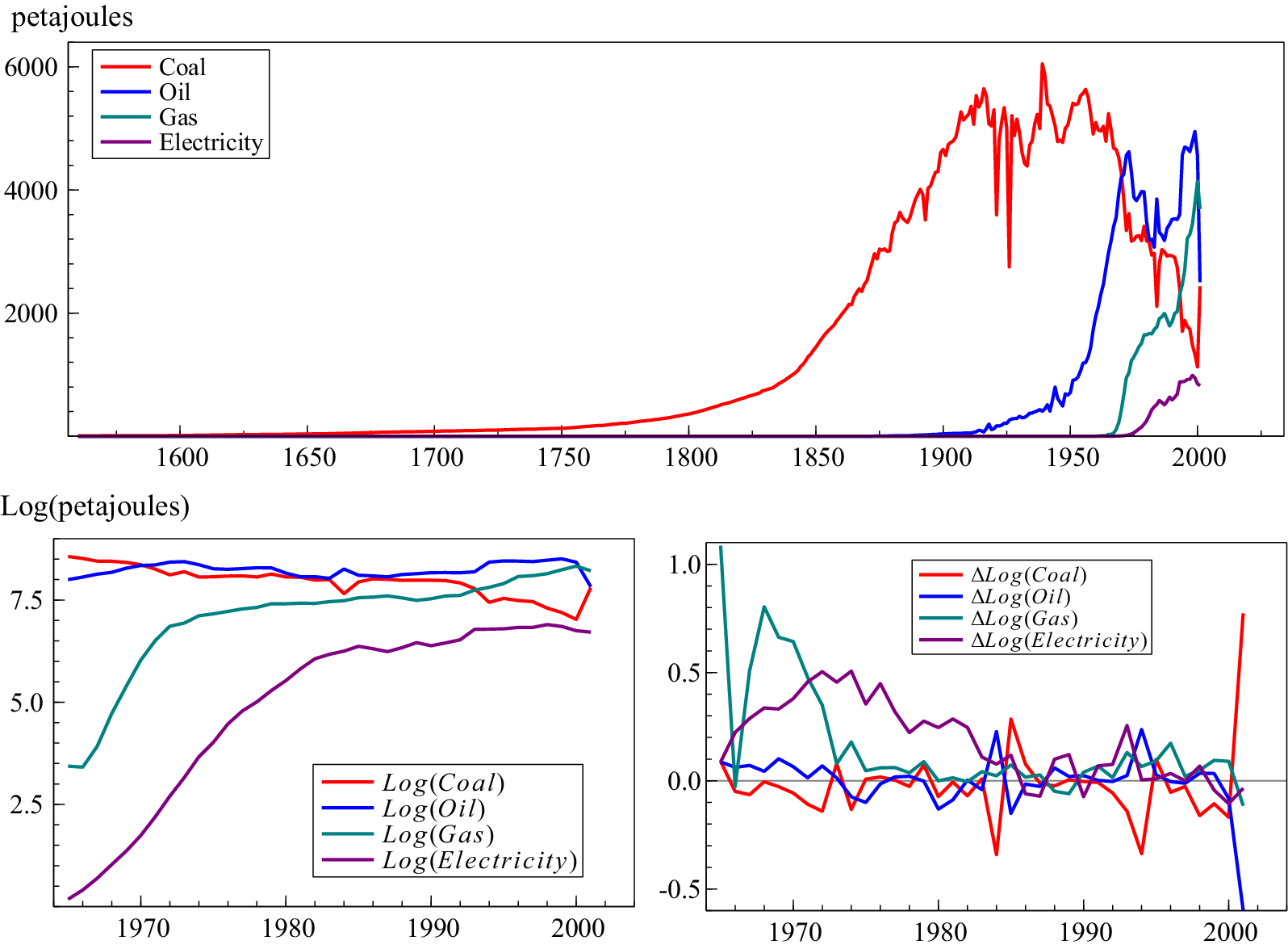
The data for modelling are taken from Warde (Reference Warde2007), recorded in Figure 3a. Data on coal, oil (petroleum), natural gas and electricity cover 95% of all fuel use, so we ignore the other fuel uses (including coke and breeze, other solid fuels, heat, bioenergy and waste), calculating percentage shares as a total of the four modelled fuels. Primary electricity as a consumption source only began in 1965, so we commence the sample in 1965 and take logs, recorded in Figure 3b, along with the growth rates in Figure 3c. The dataset ends in 2001, so we estimate the model over 1966–2001 and then forecast the period 2002–2024 (the ratio of out-of-sample to in-sample is 0.64).
(a) Composition of energy consumption for the four main sources including coal, oil, natural gas and primary electricity (a subset of Figure 1c); (b) log of coal, oil, natural gas and primary electricity consumption for the UK, 1965–2001; (c) change in log coal, oil, natural gas and primary electricity consumption for the UK, 1965–2001.

Figure 3. Long description
The figure consists of three panels.
Top panel: A line graph showing energy consumption in petajoules from the year 1560 to 2000. The y-axis ranges from 0 to 6000. Coal (red) shows a long-term exponential increase starting around 1750, peaking near 6000 petajoules in the early 1900s, followed by a volatile decline. Oil (blue) and Gas (teal) show rapid increases starting after 1950. Primary electricity (purple) shows a gradual rise starting around 1970.
Bottom-left panel: A line graph showing the log of petajoules from 1965 to 2001. The y-axis ranges from 2.5 to 7.5. Log Coal (red) and Log Oil (blue) remain relatively high and stable with slight fluctuations. Log Gas (teal) and Log Electricity (purple) show steep upward slopes before leveling off toward the year 2000.
Bottom-right panel: A line graph showing the change in log consumption (Delta Log) from 1965 to 2001. The y-axis ranges from negative 0.5 to 1.0. The data represents annual fluctuations around a zero-baseline. Delta Log Coal (red) and Delta Log Oil (blue) show significant downward spikes near 2000, while Delta Log Gas (teal) and Delta Log Electricity (purple) show higher volatility in the early years (1965 to 1980) before stabilizing closer to the zero line.
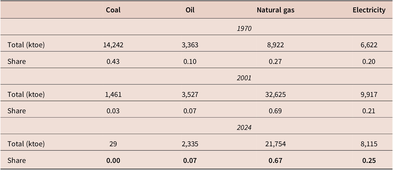
The most recent data that we have to evaluate the forecasts come from the Department for Energy Security & Net Zero statistics on Energy Consumption in the UK 2025. Table 1 summarises UK domestic consumption of energy measured in kilotonnes of oil equivalent (ktoe). To use these statistics to evaluate the forecasts, we convert to usage shares over the four components, allowing us to forecast in log(petajoule) units. The shares highlighted in the final row are the benchmark shares that we shall evaluate the forecasts against.
UK domestic consumption of energy. Bold indicates the benchmark shares that forecasts are evaluated against.

Table 1. Long description
The table compares energy consumption across four categories.
For 1970:
* Coal: 14,242 k t o e (0.43 share).
* Oil: 3,363 k t o e (0.10 share).
* Natural gas: 8,922 k t o e (0.27 share).
* Electricity: 6,622 k t o e (0.20 share).
For 2001:
* Coal: 1,461 k t o e (0.03 share).
* Oil: 3,527 k t o e (0.07 share).
* Natural gas: 32,625 k t o e (0.69 share).
* Electricity: 9,917 k t o e (0.21 share).
For 2024:
* Coal: 29 k t o e (0.00 share).
* Oil: 2,335 k t o e (0.07 share).
* Natural gas: 21,754 k t o e (0.67 share).
* Electricity: 8,115 k t o e (0.25 share).
The data shows a significant shift from coal dominance in 1970 to natural gas dominance by 2001 and 2024.
Source: Department for Energy Security & Net Zero statistics on Energy Consumption in the UK 2025 https://www.gov.uk/government/statistics/energy-consumption-in-the-uk-2025.
5.1. Modelling approach
We build a multivariate vector autoregressive model of the four energy uses. The data are highly non-stationary with possible outliers, structural breaks and non-linearities so we use saturation estimation with automatic model selection to address the wide-sense non-stationarities present, see Hendry and Doornik (Reference Hendry and Doornik2014). The initial model specification is given by:

where
$ \boldsymbol{\Upsilon} \sim \mathrm{IN}\left[\mathbf{0},\boldsymbol{\Omega} \right] $
 and we define the vector of endogenous variables as

$ \tilde{t} $
 is a linear deterministic trend, where
$ {\tilde{t}}^2={\left(\tilde{t}-\overline{\tilde{t}}\right)}^2-\overline{\left({\left(\tilde{t}-\overline{\tilde{t}}\right)}^2\right)} $
 . This ‘double demeaning’ (where
$ \overline{\cdot} $
 denotes the mean of
$ \cdot $
 ) reduces collinearity. The same adjustment is made for the cubic function of the deterministic trend,
$ {\tilde{t}}^3 $
 .
$ {\mathbf{1}}_4 $
 is a
$ \left(4\times 1\right) $
 vector of ones to allow for varying trends across the four endogenous variables.
Three sets of saturation indicators are included: impulse indicators (see Hendry et al. (Reference Hendry, Johansen and Santos2008) and Johansen and Nielsen (Reference Johansen, Nielsen, Castle and Shephard2009)) designed to detect outliers, denoted
$ {I}_{year} $
 , step indicators (see Castle et al. Reference Castle, Doornik, Hendry and Pretis2015) designed to model location shifts and denoted
$ {S}_{year} $
 and trend indicators (see Castle et al. Reference Castle, Doornik, Hendry and Pretis2025) used to model breaks in trends, denoted
$ {\tau}_{year} $
 . Steps end at the given date, and trends are specified as commencing at
$ -t+1 $
 and ending at
$ 0 $
 and are therefore
$ 0 $
 over the forecast period. As such, none of the saturation indicators extend into the forecast horizon, so the forecasts only extrapolate the trend functions. Saturation is initially applied at the system level, so significant indicators in one equation are retained in all equations, but we undertake a further reduction after the selection of the indicators to a simultaneous equation system in which only indicators significant in the given equation are retained.
The sample size is 36, resulting in a hugely overparameterised model, so selection is undertaken at very tight significance levels. We set the selection significance level to
$ \alpha =0.0001 $
 (see Doornik, Reference Doornik, Castle and Shephard2009) ensuring that diagnostic testing is undertaken. Given such a tight significance level, the probability of retaining an irrelevant regressor is negligible. The intercept and deterministic trend are set as unrestricted regressors so are not selected over, but the non-linear trend functions are selected over. Once a reduced-form unrestricted model is obtained, we estimate a simultaneous equation model, applying further reductions to result in the final parsimonious model specification reported in (1).

The model is mostly well-specified, with Table 2 recording the single equation and system diagnostic tests along with the equation standard errors. The model passes all diagnostic tests apart from some evidence of heteroskedasticity in the
$ L(Oil) $
 equation and weak evidence of autocorrelation in the
$ L(Gas) $
 equation. All system tests pass comfortably. The equation standard errors reflect a well-specified model compared to data standard errors over the same period of
$ 0.36 $
 for
$ L(Coal) $
 ,
$ 0.16 $
 for
$ L(Oil) $
 ,
$ 1.27 $
 for
$ L(Gas) $
 and
$ 2.18 $
 for
$ L(Electricity) $
 .
Equation standard errors, single equation and vector diagnostic tests

Table 2. Long description
The table consists of six columns and five data rows.
Column headers from left to right are:
1. Variable name.
2. Sigma hat (standard error).
3. F sub a r.
4. F sub a r c h.
5. Chi-squared sub n d.
6. F sub h e t.
Data rows:
- L open parenthesis Coal close parenthesis: 0.043, 0.59 [0.56], 0.97 [0.33], 0.07 [0.96], 1.35 [0.26].
- L open parenthesis Oil close parenthesis: 0.045, 2.04 [0.15], 0.05 [0.83], 1.27 [0.53], 4.34 [0.002] followed by two asterisks.
- L open parenthesis Gas close parenthesis: 0.050, 3.61 [0.04] followed by one asterisk, 0.03 [0.86], 0.01 [0.99], 2.04 [0.07].
- L open parenthesis Electricity close parenthesis: 0.069, 1.46 [0.25], 1.28 [0.27], 2.07 [0.36], 1.59 [0.18].
- System: No value for sigma hat, 0.90 [0.63], 0.99 [0.47], 6.93 [0.54], no value for F sub h e t.
Note: One asterisk denotes significance at the 5 percent level and two asterisks denote significance at the 1 percent level.
Note: *denotes significance at the 5% level and ** at the 1% level.
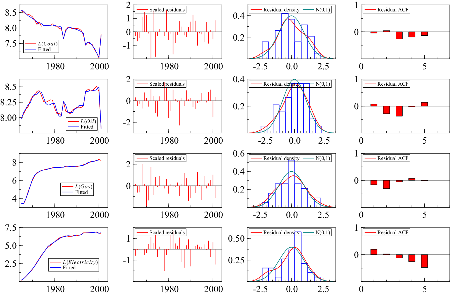
Figure 4 records the model fit, residuals, residual density and residual autocorrelation function. Coal does not depend on other energy sources. Other than its lag, the decline in coal is well captured by a combination of the linear and non-linear deterministic trends with a significant outlier in the last observation, 2001, which must be modelled explicitly to avoid forecasting from the wrong initial condition. The large increase in coal in 2001 was due to the price of natural gas rising sharply relative to coal. The electricity market conditions temporarily made coal-fired generation more profitable. Furthermore, some nuclear generation capacity was unavailable due to outages and maintenance. As existing coal stations were still available and could ramp generation back up quickly, the generators switched back toward coal for a short period.Footnote 3 We treat 2001 as an outlier in the forecasting model, just at the forecast origin.
Model fit, residuals, residual density and residual autocorrelation function.

Figure 4. Long description
The figure consists of four rows and four columns.
Row 1 (Coal):
- Panel 1: Line graph of L (Coal) and Fitted values showing a downward trend from 8.5 to 7.5 with sharp fluctuations.
- Panel 2: Scaled residuals bar chart showing random distribution around zero.
- Panel 3: Residual density histogram with a red curve and a green N (0, 1) normal distribution curve centered at 0.0.
- Panel 4: Residual A C F bar chart showing low autocorrelation across 5 lags.
Row 2 (Oil):
- Panel 1: Line graph of L (Oil) and Fitted values showing a cyclical pattern between 8.0 and 8.5.
- Panel 2: Scaled residuals showing higher variance than coal.
- Panel 3: Residual density histogram closely following the normal distribution curve.
- Panel 4: Residual A C F showing a significant negative spike at lag 3.
Row 3 (Gas):
- Panel 1: Line graph of L (Gas) and Fitted values showing a steep logarithmic increase from 4 to 8.
- Panel 2: Scaled residuals showing consistent variance.
- Panel 3: Residual density histogram with a high peak at 0.0.
- Panel 4: Residual A C F showing small negative values at lags 1 and 2.
Row 4 (Electricity):
- Panel 1: Line graph of L (Electricity) and Fitted values showing a smooth asymptotic increase from 0 to 7.5.
- Panel 2: Scaled residuals showing random noise.
- Panel 3: Residual density histogram slightly skewed to the right.
- Panel 4: Residual A C F showing a downward trend in autocorrelation from lag 1 to lag 5.
Oil depends on lagged electricity as well as lagged oil, reflecting a degree of substitutability, with a non-linear deterministic trend. There are some outliers but not for the 1970s oil crises, which suggests a degree of ‘locked in’ consumption where it is difficult to substitute energy source at short notice given the investment in domestic infrastructure needed to switch. Gas depends on oil and electricity as well as lagged gas, although all with positive coefficients. In 1971, North Sea gas production scaled up significantly, leading to both a step change and a trend increase in gas consumption.
Finally, electricity only has dynamics coming from lagged electricity, and other than a trend break in 1977, the trend is linear for log(electricity), suggesting that electricity consumption is growing exponentially. This will be the key driver of the forecasts.
5.2. Forecasting energy consumption shares
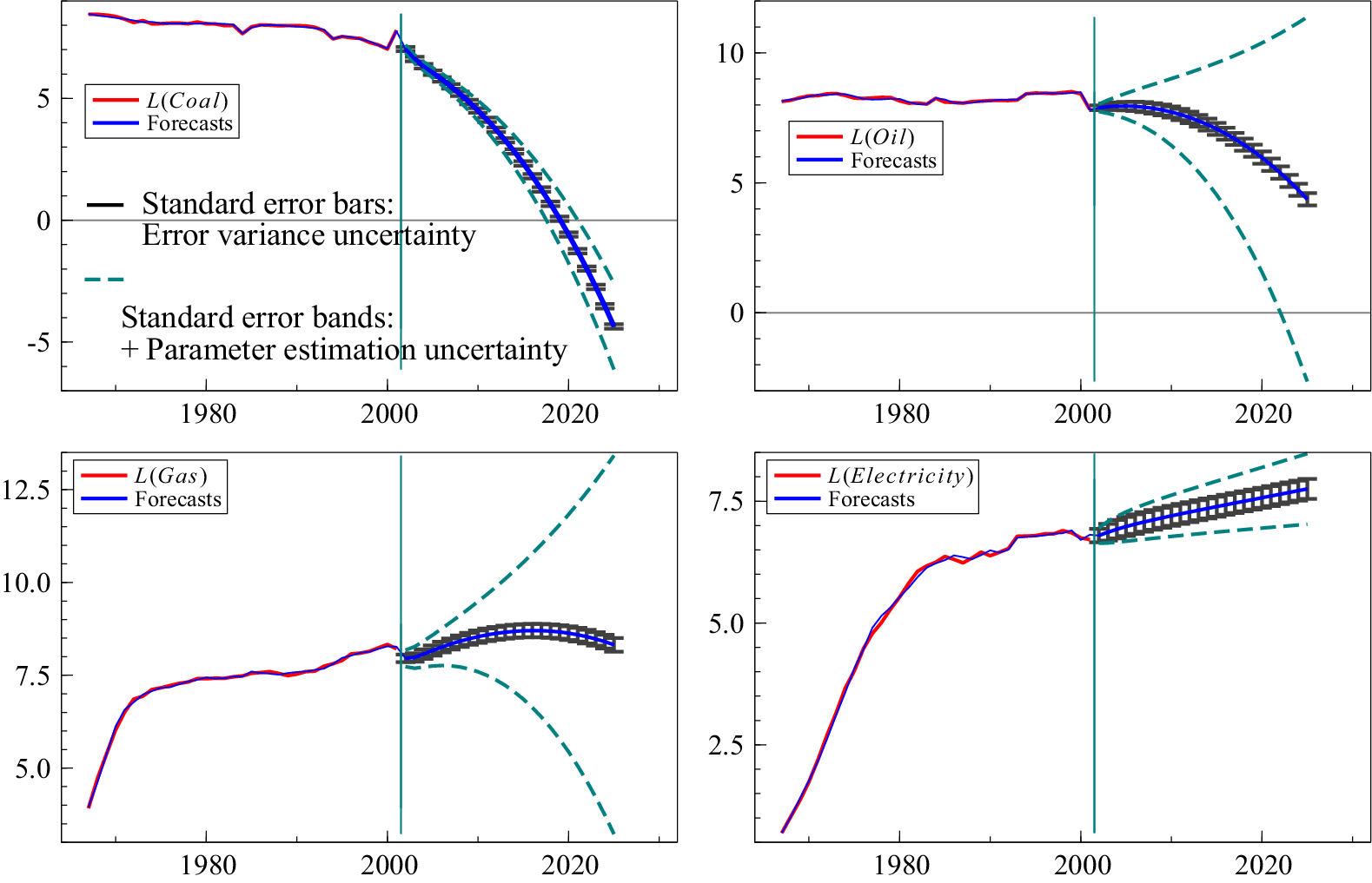
As the system is closed with deterministic linear and non-linear trends, model (1) can be used to forecast as far into the future as required. Despite only estimating the model on 36 observations, we forecast 23 periods ahead to 2024, the most recent year in which we have domestic energy consumption data. To reflect the large out-of-sample relative to in-sample observations, we report both the error variance uncertainty and the error variance and parameter estimation uncertainty. The much wider forecast error bands highlight the inherent uncertainty over the long forecast period. The error bands do not reflect uncertainty associated with structural breaks.
Figure 5 records the dynamic forecasts for
$ {\hat{\boldsymbol{y}}}_{T+h\mid T} $
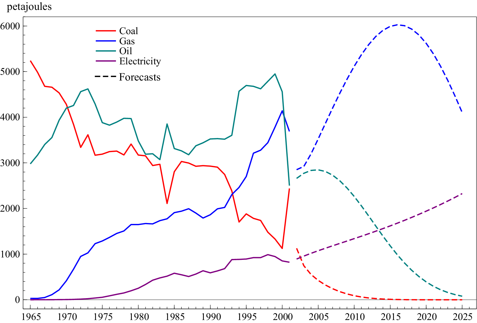
 and Figure 6 records the forecasts from (1) transformed to levels in petajoules, highlighting the very different trajectories across the energy mix. Coal converges to 0, oil is declining but at a less rapid rate, gas is non-linear but is starting to decline by the end of the forecast period and electricity is continuing its linear growing trajectory.
Dynamic forecasts for
$ {\hat{\boldsymbol{y}}}_{T+h\mid T} $
 over 2002–2024 including (a)
$ L(coal) $
 ; (b)
$ L(oil) $
 ; (c)
$ L(gas) $
 ; and (d)
$ L(electricity) $
 . Error variance uncertainty given by grey bars, and dashed green bands include parameter estimation uncertainty.

Figure 5. Long description
A multi-panel figure containing four line graphs labeled a through d. Each graph features a vertical teal line at the year 2002, separating historical data (red line) from dynamic forecasts (blue line). Grey horizontal error bars indicate error variance uncertainty, and dashed green bands represent parameter estimation uncertainty.
* Panel A, L (coal): The historical data shows a slight decline from 1980 to 2002. The forecast shows a sharp, accelerating downward curve, dropping from approximately 7 in 2002 to below -4 by 2024. The dashed green uncertainty bands widen significantly as time progresses.
* Panel B, L (oil): Historical data remains relatively stable around 8. The forecast shows a gradual decline starting after 2002, reaching approximately 5 by 2024. The dashed green bands diverge sharply, with the upper band rising above 10 and the lower band dropping toward -2.
* Panel C, L (gas): Historical data shows a steady increase from 4 in 1980 to over 7.5 in 2002. The forecast shows a slight further increase followed by a plateau around 8.5. The dashed green uncertainty bands diverge symmetrically, spanning from 3 to 13 by 2024.
* Panel D, L (electricity): Historical data shows a rapid linear increase from 1 in 1980 to nearly 7 in 2002. The forecast continues this upward trend at a shallower slope, reaching approximately 8 by 2024. The dashed green bands remain relatively narrow compared to the other panels, following the upward trajectory of the forecast.
Dynamic forecasts for
$ {\hat{\boldsymbol{Y}}}_{T+h\mid T} $
 including coal, oil, gas and electricity over 2002–2024.

Figure 6. Long description
The x-axis represents years from 1965 to 2025. The y-axis represents energy in petajoules from 0 to 6000. Historical data is shown as solid lines until 2002, followed by dashed lines for forecasts.
* Coal (red line): Starts at approximately 5200 petajoules in 1965, showing a long-term decline with significant volatility, dropping to around 1100 by 2000. The forecast shows a rapid decline toward zero by 2015.
* Gas (blue line): Starts near zero in 1965, showing a steady linear increase to 4000 petajoules by 2000. The forecast predicts a sharp parabolic rise peaking at 6000 petajoules around 2017 before declining to 4100 by 2025.
* Oil (teal line): Starts at 3000 petajoules, fluctuates with peaks near 5000 in 1975 and 1998. The forecast shows a peak at 2800 in 2005 followed by an asymptotic decline toward zero by 2025.
* Electricity (purple line): Starts near zero and shows a slow, steady increase to 1000 petajoules by 2000. The forecast predicts a continued linear increase reaching approximately 2300 petajoules by 2025.
To evaluate the accuracy of the forecasts, we calculate the energy consumption shares in 2024, recorded in Table 3 along with the actual shares reported in Table 1. The model estimated up to 2001 is able to accurately forecast energy consumption shares 23 years later despite only modelling the trends over a 36-year period, which contains many breaks, outliers and non-linearities. The estimate for oil is slightly too low, and the share for electricity is slightly too optimistic, but overall, allowing for non-linear deterministic trends and saturation indicators resulted in a well-specified model that could forecast energy shares reasonably accurately.
Forecast energy consumption shares in 2024 (23 step ahead dynamic forecast) compared to actual shares (excluding negligible energy mix components)

Table 3. Long description
The table consists of four columns representing energy sources and two rows representing data types.
Header Row: Coal, Oil, Gas, Electricity.
Row 1: Forecast share.
- Coal: 0.00
- Oil: 0.02
- Gas: 0.65
- Electricity: 0.33
Row 2: Actual share.
- Coal: 0
- Oil: 0.07
- Gas: 0.67
- Electricity: 0.25
The data shows that Gas is the dominant energy source in both forecast and actual shares, while Coal has been phased out to zero.
5.3. An unrealistic counterfactual
If the climate crisis was to be avoided, the UK would have needed to transition away from coal more than a century ago. Given that the knowledge and understanding of electricity, its applications and the costs of burning fossil fuels were all known by 1900, we take this as a fork in the road in which the economy could have gone down an all-electric path. This is a far-fetched assumption given the Victorians thought it would take thousands of years for humanity to double atmospheric CO2 through fossil fuel use, and they did not have a framework to quantify the economic damages of climate change. Nevertheless, it is an instructive counterfactual to see how rapidly we could have taken a different path.
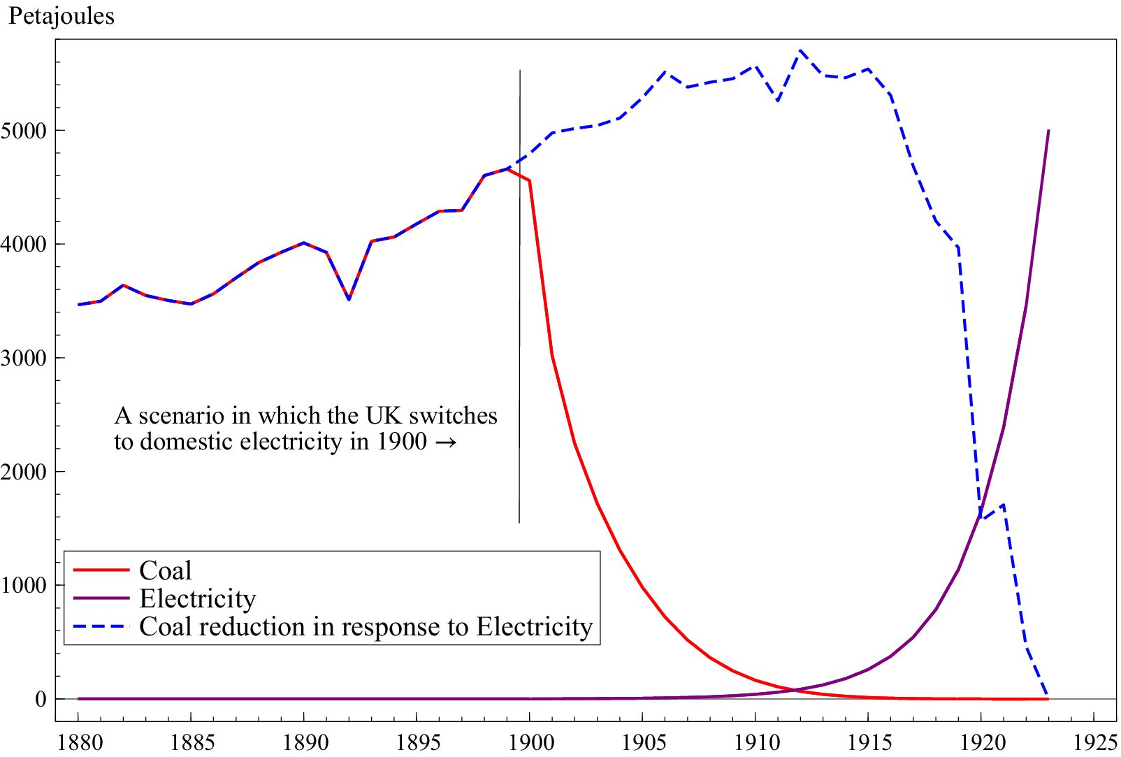
We take the forecasts over the period 2002–2024 and map them to the data in 1900. We ignore oil and gas as they constituted 0.8% and 0% of energy consumption in 1900 respectively. Figure 7 records the projections for coal and electricity. The scenario projection for coal is based on the non-linear trends from (1) (solid red line), and the trajectory for electricity is due to the linear
$ L(Electricity) $
 model, resulting in exponential growth in electricity, with the projection bounded by total energy consumption in petajoules in 1924 (solid maroon line).
A scenario for coal and electricity consumption in 1900 had the UK gone down an electric energy path.

Figure 7. Long description
The X axis represents years from 1880 to 1925. The Y axis represents energy in Petajoules from 0 to over 5000. A vertical line marks the year 1900 with the text: A scenario in which the U K switches to domestic electricity in 1900 followed by a right-pointing arrow.
Data Series:
* Coal (solid red line): Shows a fluctuating increase from 3500 Petajoules in 1880 to a peak of approximately 4700 in 1900. After 1900, it follows a steep exponential decay, reaching near zero by 1915.
* Electricity (solid purple line): Remains at zero from 1880 until approximately 1908, after which it shows an exponential increase, reaching 5000 Petajoules by 1923.
* Coal reduction in response to Electricity (dashed blue line): This line tracks with the Coal line until 1900. After 1900, it continues to rise to a peak of nearly 5800 Petajoules around 1912, then fluctuates and sharply declines to zero by 1923, representing the counterfactual coal usage.
There are numerous assumptions embodied in this simple counterfactual exercise, but it is designed to demonstrate the speed of adjustment despite sunk costs in domestic consumption of energy. The scenario assumes that oil and gas were not developed and electricity directly replaced coal as the dominant source of energy consumption, but we are in a more complicated world where we need to transition away from natural gas towards green electricity generation. Furthermore, the scenario assumes the rate of transition at the beginning of the 21st century. Clearly, this would have been infeasible because substitution from coal to electricity would need to match, so the reduction in coal would be much slower initially as electricity takes time to establish. For example, in 1912, the total consumption of energy would have been 150 petajoules under this scenario, whereas the total consumption in 1912 was 5345 petajoules. To address this constraint, we also record the coal trajectory based on the speed of electricity adoption, calculated as the difference between total energy consumption in a given year and the electricity energy consumption (dashed blue line). Under this more realistic scenario, coal is replaced much more gradually initially, but once the transition takes hold, the exponential nature of electricity consumption drives the rapid reduction in coal.
While obvious fiction, connections to reality abound. Local urban grids would have sufficed initially given the energy demands of the time, gradually expanding and linking to accrue the benefits of standardisation and larger markets. What became filling stations could have wind turbines with battery storage to supply rural areas and longer distance driving. Given their huge efficiency and ability to both warm and cool as seasons changed, heat pumps would have been an attractive proposition and obviated the need for gas boilers and electric immersion water heaters. Solar panels would have improved and supplied local power, including for industry noting the rapid increase to almost 80% in the share of horsepower from electric motors in US manufacturing between 1898 and 1925 (see Hall, Reference Hall, Fagerberg, Mowery and Nelson2005, Figure 1). The examples of efficient electric trams and underground trains suggest these would gradually supplant steam trains, although propulsion for large ships by coal-driven steam would probably have persisted with smaller boats driven by electric motors. We can only conjecture on how flight might have evolved in an all-electric world.
The main weakness is that electricity generation would have relied heavily on coal-fired power stations until more highly efficient alternatives evolved.
6. Conclusions
We document the incredible depth and breadth of knowledge on electricity in the 19th century, including its generation and its uses, from batteries and generators to motors and photovoltaic solar cells and heat pumps. Furthermore, it was understood that CO2 was a GHG and burning fossil fuels resulted in CO2. As such, we came close to an all-electric world which would have avoided the climate crisis that we are now in. But humanity followed the fossil fuel path. We discuss why this was the case, highlighting externalities, market failures, sunk costs and coordination failures. Looking back at history is informative in that we can draw lessons from those failures as to how to best transition to a net-zero economy. Policy is just as crucial as technology in ensuring a shift towards green energy consumption. Now the transition has taken hold, a key driver will be the economics. The price of solar PV has fallen more rapidly than almost any major energy technology in history, with China playing the dominant role. Such favourable economics take on momentum.
The empirical example models the energy mix over the latter part of the 20th century. A remarkably simple model is able to capture non-linear trends, outliers and structural breaks in wide-sense non-stationary data. True ex ante dynamic forecasts are made over 23 years, producing energy consumption shares close to those that are currently observed. Although oil is a small component of domestic consumption, it is stubbornly persistent and will need policy intervention to phase out completely. The next challenge for the UK is to transition away from natural gas towards green electricity, which requires reform of the UK electricity pricing market, and external shocks such as the war in Iran are highlighting the need for UK energy resilience, which goes hand in hand with the net-zero transition.
The scenario projection demonstrates that an electric world would have been feasible. An all-electric future where we might have been did not take off, but had it done so, GDP would have generated few GHGs, and the climate crisis would not be upon us.
Acknowledgements
We thank participants of the NIER Workshop on the Economics of Climate Change and the Climate Transition, and in particular Richard Clarke, for comments on an earlier draft. All calculations and graphs use PcGive and OxMetrics.
Funding statement
The research was supported by NSF grant BCS-2234914 and NIH/NIDCD grant R01DC017162.
Competing interests
Jennifer L. Castle and David F. Hendry declare that they have no known financial or personal competing interests that could have appeared to influence the work reported in this paper.
Data availability statement
Historical data on energy consumption and energy intensity for the UK from 1560 from Warde (Reference Warde2007) are available to download from https://histecon.fas.harvard.edu/energyhistory/data/Warde_Energy_%20Consumption%20England.pdf.
Energy consumption in the UK from 1970 is available from the Department for Energy Security & Net Zero Energy Consumption in the UK 2025 https://www.gov.uk/government/statistics/energy-consumption-in-the-uk-2025.
Fuel input for electricity generation in the UK from 1920 is available from the Department for Energy Security & Net Zero Historical electricity data https://www.gov.uk/government/statistical-data-sets/historical-electricity-data.






 Open access

