2.1. Governing equations and linear stability approach

We consider a two-dimensional flow inside a rectangular cavity of aspect ratio $A_v=H/W$ with cavity height $H$ and width $W$, adiabatic top and bottom boundaries and the two walls kept at a constant temperature with temperature difference $\Delta T$ (see figure 1a). The scales of this problem are $\Delta T$ for the temperature difference and for the length scales $(x,y) \sim (\delta _{T},H)$, where $\delta _{T} = (\kappa t_r)^{1/2}$ is the thickness of the heated boundary layer, and $t_r$ is the reference time defined below. Using the momentum equations, the friction term then scales with the buoyancy term, i.e. $\nu V_r/(\delta _{T})^{2} \sim g \beta \Delta T$, which yields a characteristic speed $V_{r} = (\kappa / H ) Ra^{1/2}$. The time scale $t_{r} = H/V_r$ is obtained from the balance between the advective term and diffusive term in the temperature equation. With these scales, one obtains for the dimensionless form of the continuity equation, Boussinesq approximation of the Navier–Stokes equations and the temperature equations, respectively,

(2.1)\begin{gather} \boldsymbol{\nabla} \boldsymbol{\cdot} \boldsymbol{v} = 0, \end{gather}

(2.2)\begin{gather} \frac{\partial \boldsymbol{v}}{\partial t} + \boldsymbol{v} \boldsymbol{\cdot} \boldsymbol{\nabla} \boldsymbol{v} =-\boldsymbol{\nabla}P + \frac{Pr}{Ra^{1/2}} {\nabla}^{2}\boldsymbol{v} + Pr \varTheta \boldsymbol{e}_{z}, \end{gather}

(2.3)\begin{gather} \frac{\partial \varTheta }{\partial t} + \boldsymbol{v} \boldsymbol{\cdot} \boldsymbol{\nabla}\varTheta = \frac{1}{Ra^{1/2}}{\nabla}^{2} \varTheta, \end{gather}

with $\boldsymbol {v}$ the velocity vector, pressure $P$ and $\varTheta$ the dimensionless temperature $(T - T_{r} )/ \Delta T$, with $T_r$ being the average temperature (here, $T_r=0$). As mentioned above, the control parameters of this flow are the Rayleigh number, Prandtl number and aspect ratio $A=H/W$, which depends on the chosen length $W$ since the height $H$ is kept constant.

Figure 1.

(a) Schematic of the problem with the walls kept at constant temperatures 0.5 and $-$0.5 so that $\Delta T = 1.0$. The initial condition for the nonlinear simulations is $T_0= \Delta T \times ( x/x_{max} - 0.5 ) + {\rm noise}$ and $(u, v) = (0,0)$, and for the linear simulations, $T_{p_0}= {\rm noise}$ and $(u_p, v_p) = (0,0)$. (b) Location of the interrogation points used to assess the state of the flow with the oscillation frequency $\omega$ measured in the corner at $(x,z)=(0.1,0.1)$, for $A=1$, $H=(0,1)$ and $W=(1,0)$, $N_c$ being the stratification in the centre of the cavity. The maximum speed in the buoyancy current is sketched by red and blue curved lines. Here, $L_h$ is the horizontal distance from the wall to the minimum (in $z$) on the red line of the current at the top.

The no-slip condition is used for all boundaries. For the temperature, the Dirichlet condition is used with $\varTheta =0.5$ and $\varTheta =-0.5$ on the two lateral walls, and for zero heat flux the Neumann condition at the two horizontal boundaries.

Numerical simulations are performed with the spectral element code Nek5000 (https://nek5000.mcs.anl.gov) using the two newly developed Python packages Snek5000 (https://snek5000.readthedocs.io) and Snek5000-cbox (https://github.com/snek5000/snek5000-cbox) (Augier, Mohanan & Bonamy Reference Augier, Mohanan and Bonamy2019; Mohanan et al. Reference Mohanan, Bonamy, Linares and Augier2019; Mohanan, Khoubani & Augier Reference Mohanan, Khoubani and Augier2023). The packages are available online and the data that we have produced here are available as a Zenodo dataset (https://zenodo.org/record/7827872).

Tests have been conducted for $Pr=0.71$ and $A=1$ and results for the growth rate and oscillation frequency have been validated with respect to former studies in the literature. The resolution employed (see table 1 in the Appendix) allows for the study of the motion in the thin boundary layers near the walls, and accuracy in growth rate and oscillation frequency. Figure 2 shows a typical temperature signal measured in the corner of the cavity (see figure 1b) for the nonlinear simulation. The large difference in temperature between figures 2(a) and 2(b) reveals the transient to the base state ($t < 250$) and the subsequent growth and saturation of the instability ($t>250$), respectively. From $t=0$ to 250, the motions along the boundaries and the stratification in the interior develop. The base state is a steady state with minimum amplitude of oscillations (at approximately $t \approx 500$), with motions in thermal boundary layers in the presence of a stratified interior. From $t = 500$ onwards, a linear instability leads to the exponential growth of the amplitude of the oscillation up until approximately $t=1375$, after which it saturates and small nonlinear oscillations in amplitude develop. The oscillation frequency shows a perfect exponential growth in the range of approximately $500< t<1400$ (see the inset in figure 2b).

Figure 2.

Temperature signal of a nonlinear simulation at point $(x, z) = (0.1, 0.1)$ for $A=1.0$, $Pr=0.71$ and $Ra = 1.85 \times 10^{8}$, with (a) the evolution of the flow from $t=0$, and (b) the evolution to a steady state and subsequent exponential growth in amplitude and saturation. The inset shows the perturbation in log scale with the fit giving the growth rate (straight line).

For each set of control parameters $Pr$ and $A$, nonlinear simulations are performed to obtain a first approximation of the critical Rayleigh number $Ra_c$. Nonlinear simulations reach a steady state at a Rayleigh number of O($\sim 10^8$) but still smaller than the critical Rayleigh number, i.e. $Ra< Ra_c$, while for slightly higher $Ra$ values, the flow starts to oscillate at $t \approx 500$. Three nonlinear simulations are performed for three values of $Ra$ slightly larger than the estimated $Ra_c$ using the selective frequency damping (SFD) method of Åkervik et al. (Reference Åkervik, Brandt, Henningson, Hœpffner, Marxen and Schlatter2006), which give us three steady base states. This method has also been used recently for computing the base state of the flow that is induced when tilting a cavity containing a stably stratified fluid (see Grayer et al. Reference Grayer, Yalim, Welfert and Lopez2020).

Subsequently, the linear stability of these steady base flows is considered. Using perturbed variables $\varTheta = \varTheta _{b} + {\theta }'$, $\boldsymbol {V} = \boldsymbol {V}_{b} + {\boldsymbol {v}}'$, $P = P_{b} + {p}'$ where subscript $b$ represents the base state and superscript ${}'$ the perturbation, and neglecting second-order terms, we obtain linearised perturbation equations of the form

(2.4)\begin{gather} \frac{\partial{\boldsymbol{v}}'}{\partial t} + \boldsymbol{V_{b}} \boldsymbol{\cdot} \boldsymbol{\nabla}{\boldsymbol{v}}' + {\boldsymbol{v}}' \boldsymbol{\cdot} \boldsymbol{\nabla} \boldsymbol{V_{b}} =-\boldsymbol{\nabla}{p}' + \frac{Pr}{Ra^{1/2}} {\nabla}^{2}{\boldsymbol{v}}' + Pr {\theta}' \boldsymbol{e}_{z}, \end{gather}

(2.5)\begin{gather} \frac{\partial{\theta}' }{\partial t} + \boldsymbol{V_{b}} \boldsymbol{\cdot} \boldsymbol{\nabla}{\theta}' + {\boldsymbol{v}}' \boldsymbol{\cdot} \boldsymbol{\nabla}\varTheta_{b} = \frac{1}{Ra^{1/2}} {\nabla}^{2} {\theta}'. \end{gather}

Linear simulations are run for the three steady base states obtained from the SFD method, and corresponding to three unstable $Ra$ values. A small amount of noise of the order of $10^{-6}$ is added so that, due to the linear instability, an exponential growth of the leading mode is observed in the whole cavity. This noise is random and therefore not necessarily symmetric. Then, the growth rate is determined for each linear simulation, thus providing eventually three different growth rates. Using a linear interpolation of these growth rates, the critical Rayleigh number $Ra_c$ is extrapolated from the value for zero growth rate. The base flow and the perturbation analysed in the next section are obtained from the nonlinear and linear simulations for the Rayleigh number just above this critical Rayleigh number.

2.2. Decomposition of the leading linear mode

In view of former observations of this instability (see e.g. Xin & Le Quéré Reference Xin and Le Quéré2006), the different variables can be decomposed during the oscillating exponential growth into

(2.6)\begin{gather} \theta'\left(x,z,t\right)= A_{\theta}(x,z) \cos\left(\omega t + \varPhi_{\theta}\left(x,z\right)\right){\rm e}^{\sigma_{r}t}, \end{gather}

(2.7)\begin{gather} u'\left(x,z,t\right)= A_{u}\left(x,z\right)\cos\left(\omega t + \varPhi_{u}\left(x,z\right)\right){\rm e}^{\sigma_{r}t}, \end{gather}

and

(2.8)\begin{equation} w'\left(x,z,t\right)= A_{w}\left(x,z\right)\cos\left(\omega t + \varPhi_{w}\left(x,z\right)\right){\rm e}^{\sigma_{r}t}, \end{equation}

where $A(x,z)$, $\omega$, $\varPhi (x,z)$ and $\sigma _{r}$ are amplitude, frequency, phase and growth rate of the field variables, respectively. The growth rate $\sigma$ and the oscillation frequency $\omega$ are computed by an algorithm based on Hilbert transforms. The amplitude fields are then obtained by taking the time maximum of the perturbation variables divided by ${\rm e}^{\sigma _{r}t}$. Finally, the phase fields are obtained with one curve fit per grid point and variable.

3.1. The steady base flow and diagnostics

Figure 3(a–f) shows the steady base flow for different Prandtl numbers and constant aspect ratio $A=2.0$. From figure 3(a–f) one notices that, for larger Prandtl numbers, the buoyancy currents detach and meander along the horizontal boundaries, the number of meanders depending on the $Pr$. Clear experimental and numerical support for this meandering is shown by Xu, Patterson & Lei (Reference Xu, Patterson and Lei2008). The wavelength of this meandering buoyancy current changes significantly with $Pr$, while its presence is limited by the horizontal extend $W$ of the cavity represented by $A$ (note $H$ is kept constant). When the width of the cavity is smaller than this wavelength, the head of the buoyancy current joins the start of the cold boundary layer, and vice versa near the bottom boundary, such that the two currents reinforce each other's inertia, leading to a large-scale fast circulation along the boundaries (see figure 3a). With increasing $Pr$ ($Pr<0.7$ in figure 3), the large-scale circulation decreases in strength and the buoyancy current detaches from the horizontal boundary, i.e. $L_h< W$, and it meanders locally. For larger $Pr$ values, ($Pr>1$, see figure 3d–f) a horizontal exchange flow establishes in the interior between the two thermal boundary layers. The boundary layers are thinner for these higher $Pr$ values. For a constant $Pr$ it depends on the aspect ratio whether there are cell patterns (as in figure 3a) or rather horizontal exchanges between the thermal boundary layers (as in figure 3f) (see Xin & Le Quéré Reference Xin and Le Quéré2006).

Figure 3.

The base flow states for $A=2.0$ and different $Pr$: (a) $Pr=0.35$, (b) $Pr=0.53$, (c) $Pr=0.71$, (d) $Pr=1.4$, (e) $Pr=2.0$ and (f) $Pr=2.8$. Streamlines are supplied with arrows indicating flow direction, and colour representing the temperature.

Figure 4 shows flows for $Pr=0.35$ and varying aspect ratio $A$. When the width of the cavity is large (see figure 4a for $A=0.5$), the buoyancy current meanders along the horizontal boundary. With increasing aspect ratio $A$, the meander length scale of the buoyancy current becomes smaller than the width of the cavity, and there is an increasing tendency for the formation of cell circulation. Two circulation cells appear for $A=2$ in figure 4(d).

Figure 4.

The base flow state for $Pr=0.35$ and different $A$: (a) $A=0.5$, (b) $A=1.0$, (c) $A=1.5$ and (d) $A=2.0$. Lines show the streamlines with the arrows giving the flow direction, and colour representing the temperature.

In all cases, a stable density gradient $-\beta d T/d z$ is present in the interior. The buoyancy (Brunt–Väisäilä) frequency scaled with time $t_r = H^2 / (\kappa {Ra}^{1/2})$ is given by

(3.1)\begin{equation} (N_c t_r)^2 = g \beta \frac{{\rm d} T}{{\rm d}z} \frac{H^4}{\kappa^2} \frac{1}{Ra} = Pr \frac{H}{\Delta T} \frac{{\rm d}T}{{\rm d}z}, \end{equation}

showing that the Prandtl number, height of the reservoir and density gradient are relevant for the scaled buoyancy frequency, with slightly stronger stratifications for shallow cavities (small $A$) and weaker stratifications for high and narrow cavities (large $A$).

In the simulations, the buoyancy frequency $N_c$ is determined by the density gradient in a small region around the centre of the tank. The meander length scale of the buoyancy current, $L_h$, is defined as the horizontal distance from the wall where the line that describes the maximum speed (see figure 1b) has a minimum in $z$. Here, $L_h$ has been determined from the flow near the top. In the perturbed state, the instability causes oscillations in the temperature with frequency, $\omega$. Its amplitude increases due to the linear instability, and although present in the entire tank, the oscillations are mainly visible in the corner regions where the thermal motion along the wall is blocked by the horizontal boundary (see e.g. Le Quéré & Behnia Reference Le Quéré and Behnia1998; Xin & Le Quéré Reference Xin and Le Quéré2006, and references therein). Thus, to analyse this flow, the frequency of the oscillation frequency of the instability mode, $\omega$, the density stratification in the interior, $N_c$ and the wavelength of the meandering buoyancy current, $L_h$, are measured at the locations shown in figure 1(b).

When the temperature oscillations have a higher frequency than the buoyancy frequency, i.e. $\omega >N_c$, internal waves cannot propagate in the interior and are evanescent. In contrast, when $\omega < N_c$, the buoyancy currents near top and bottom boundaries may couple due to the internal waves that propagate into the interior. Even though a larger value of $N$ may exist near the top and bottom boundaries, the value $N_c$ in the centre of the tank is taken as reference value since it is more relevant for the coupling of the top and bottom regions. As mentioned, flows with $\omega /N_c>1$ are called fast, and flows with $\omega /N_c<1$ slow since they allow for the propagation of internal gravity waves, and, in most cases, for the coupling between the two buoyancy currents. In the absence of internal waves, top and bottom instabilities generally start to grow independently with different perturbation amplitudes, resulting in asymmetry. This is referred to as amplitude asymmetry, or asymmetry in short, and is further detailed below.

For the base states, figure 5(a) shows the (scaled) wavelength of the meandering buoyancy current $L_h/H$ against $Pr$ for different aspect ratios of the cavity. For small $Pr$ there is no detachment and $L_h$ is larger than the width of the cavity, i.e. $L_h=1/A$. In this case, the horizontal buoyancy currents and boundary layers at the sidewalls reinforce each other, leading to a large cell circulation. For larger $Pr$ values, the boundary layers are thin and the aspect ratio $A$ has no influence on the value of $L_h/H$. The effects obtained for decreasing $Pr$ can also be obtained for larger aspect ratio. Boundary layers grow with distance and become thicker and have more inertia, leading to relatively larger values of $L_h$.

Figure 5.

(a) Meander length scale $L_h/H$ against Prandtl number, $Pr$, with the dashed lines representing the aspect ratios $A=H/W$, and (b) $N_c$, the Brunt–Väisälä frequency, scaled with the characteristic time $t_r$ at the centre of the cavity as a function of $Pr$. For comparison, the slope of $\sqrt {Pr}$ predicted by (3.1) is shown by the dashed line.

Figure 5(b) shows that the stratification in the interior increases less for $Pr>0.4$ than for $Pr<0.4$ since larger gradients form near the horizontal boundaries, and a weaker stratification forms in the interior. The aspect ratio $A$ has an influence on the internal stratification only for smaller Prandtl numbers for which the large cell circulation dominates.

The asymmetry in the value of the amplitude between the top and bottom currents is considered in particular since its relation to the presence of internal waves is novel and provides new insights. For both currents the growth rates are the same, but due to an asymmetry in the initial noise, the amplitudes of the perturbations may be different. Writing out the equations for the temperature, we have then

(3.2)\begin{equation} \theta' (\boldsymbol{x},t) = \left( C_+A_+(\boldsymbol{x}) +C_- A_-(\boldsymbol{x}) \right) \cos(\omega t + \phi (\boldsymbol{x})) \,{\rm e}^{\sigma t}, \end{equation}

with the ratio $C_+/C_-$ depending on the initial noise. Thus, in contrast to the coupled case, with top and bottom currents having the same amplitude and internal waves being part of the same global mode, we have in the uncoupled case two local regions that are growing independently.

The symmetry conditions are imposed by the boundary conditions, so that for a solution $\varPhi$ with

(3.3)\begin{equation} \varPhi(\boldsymbol{x})= \begin{pmatrix} \varTheta_b(\boldsymbol{x})\\ \boldsymbol{V_b}(\boldsymbol{x}) \\ P_b(\boldsymbol{x}) \\ \xi_b(\boldsymbol{x}), \end{pmatrix} \end{equation}

with $\xi _b=\boldsymbol {\nabla } \times \boldsymbol {V_b}$ the vorticity in the basic state, the equations are invariant for the transformations

(3.4)\begin{equation} R\varPhi(\boldsymbol{x})= \begin{pmatrix} -\varTheta_b(\boldsymbol{-x})\\ -\boldsymbol{V_b}(\boldsymbol{-x}) \\ P_b(\boldsymbol{-x}) \\ \xi_b(\boldsymbol{-x}). \end{pmatrix} \end{equation}

In case there is symmetry, the solution can be either ‘centro-symmetric’, i.e. $R\varPhi (\boldsymbol {x})=\varPhi (\boldsymbol {x})$, or ‘anti-centro-symmetric’, i.e. $R\varPhi (\boldsymbol {x})=-\varPhi (\boldsymbol {x})$ (see Burroughs et al. Reference Burroughs, Romero, Lehoucq and Salinger2004). Counter-intuitively, for centro-symmetry, the velocity phase must be opposite to that in the other corner whereas the vorticity must be equal, and vice versa for anti-centro-symmetry. This centro-symmetry was tested considering the point reflected value with respect to the centre of the tank. Thus, the non-dimensional temperature in the top half of the cavity $\theta '_{{top}}$ is compared with its flipped counterpart in the bottom half of the cavity $\theta _{{bot}}^{'{flip}}$. The parameters for centro-symmetry and anti-centro-symmetry then become, respectively,

(3.5)\begin{gather} I_C = \frac{\left\langle \left| \theta'_{{top}} - \theta_{{bot}}^{' {flip}} \right| \right\rangle}{\sqrt{\langle\theta'^2\rangle}}, \end{gather}

(3.6)\begin{gather} I_A = \frac{\left\langle \left| \theta'_{{top}} + \theta_{{bot}}^{' {flip}} \right| \right\rangle}{\sqrt{\langle\theta'^2\rangle}}, \end{gather}

with the brackets standing for the average over the domain, and the enumerator representing the root-mean-square value of $\theta '$. When the perturbation is centro-symmetric or anti-centro-symmetric, either $I_C$ or $I_A$, respectively, is small and never zero because of numerical noise. Both values are large when there is no such symmetry. To identify centro-symmetry, the difference of the reciprocals of $I_C$ and $I_A$

(3.7)\begin{equation} I_{dif} = \frac{1}{I_C} - \frac{1}{I_A}, \end{equation}

is used, with anti-centro-symmetry for $I_{dif} > 0$, i.e. the temperature perturbations in the top and bottom halves of the cavity have the same sign, and centro-symmetry for $I_{dif} < 0$, i.e. opposite temperature perturbations in the top and bottom halves of the cavity. When $I_{dif} \simeq 0$, there is no symmetry, i.e. the top and bottom currents are asymmetric in amplitude. The expression (3.7) therefore provides simultaneously information about centro-symmetry and amplitude symmetry.

Centro-symmetry is generally better solved with different methods that provide a continuous distribution for the critical Rayleigh number and the centro-symmetry as a function of Prandtl number (see e.g. Lyubimova et al. Reference Lyubimova, Lyubimov, Morozov, Scuridin, Hadid and Henry2009, and references therein). Since this was not the aim of the present investigation, the centro-symmetry below is provided for completeness, and the details are left for future study.

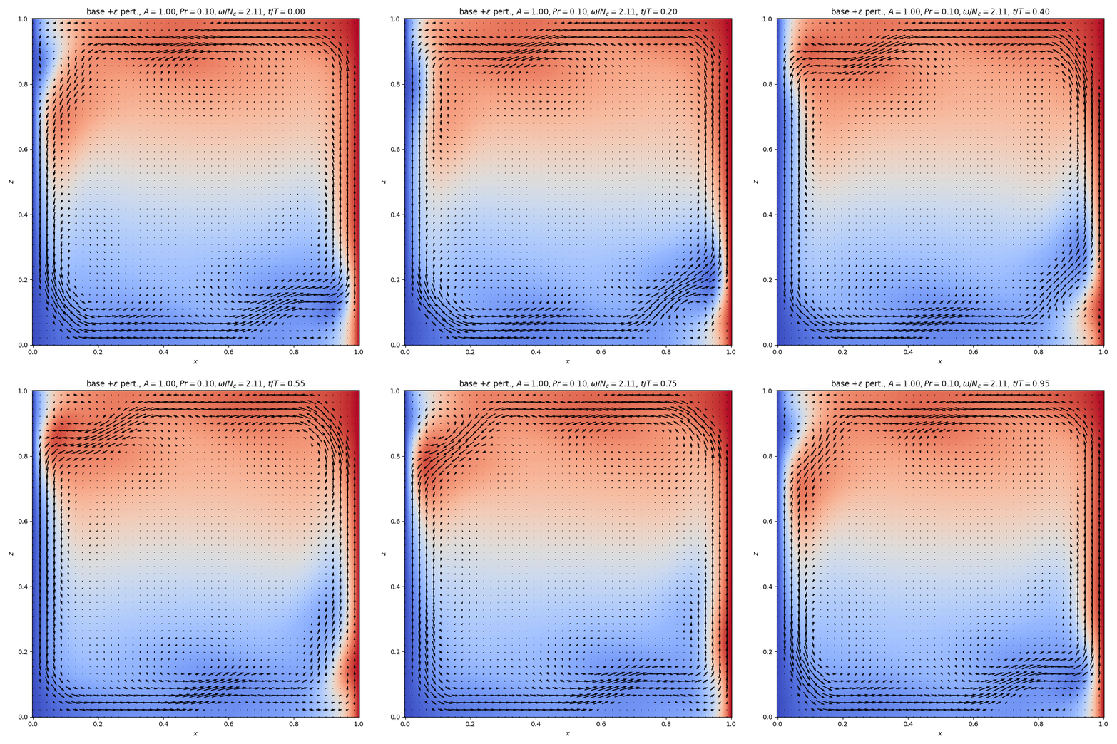
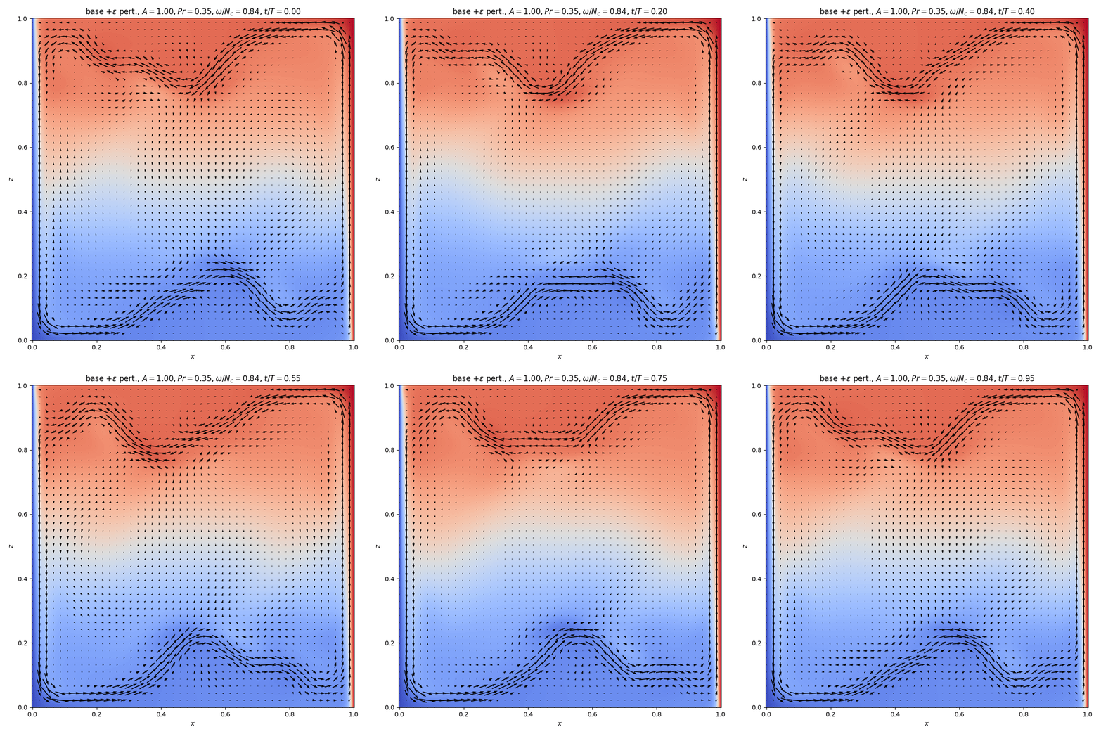
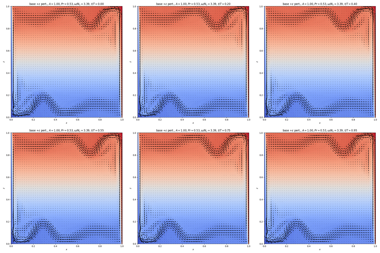
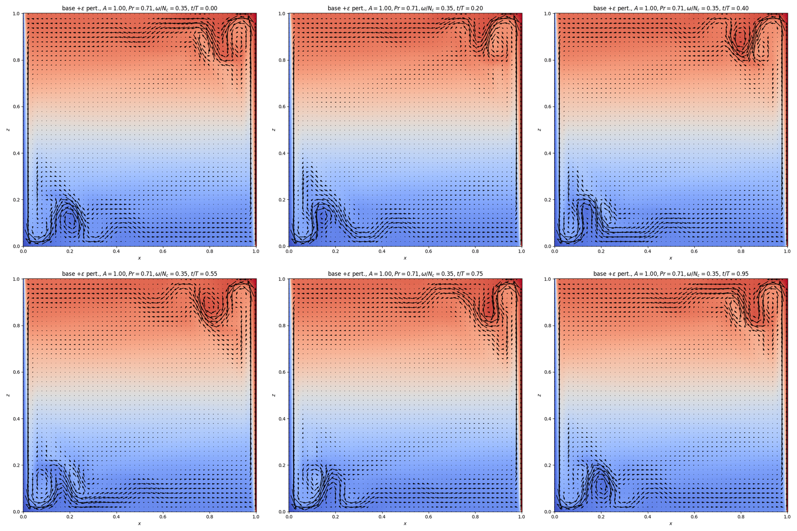
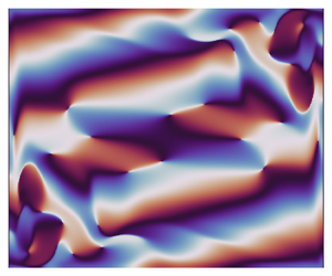
Below, the six observed regimes for increasing $Pr$ are discussed for a single aspect ratio $A=1$. For the regimes shown in figure 6 the field of the base flow is shown next to the fields of the perturbations predicted by the linear mode decomposition, with (b) amplitude, (c) phase and (d) vorticity. The perturbation of the vorticity field (d) reveals the spatio-temporal nature of the disturbing wave packets. The phase map (c) shows the distribution of the length scales in the field and can be considered as a signature of the internal waves. In addition, two time steps show the base flow perturbed with the linear perturbation (see figure 7a,b).

Figure 6.

Flow maps for $A=1.0$ and different different values of Prandtl number, $Pr$, and oscillation frequency, $\omega /N_c$ (cases I–VI), with (a) base state, (b) temperature amplitude $A_{\theta '}$, (c) phase map $\varPhi _{\theta '}$ and (d) vorticity perturbation $\xi '$. Supplementary movies of the regimes I, fast circulation cells (FCc) (movie 1); II, slow circulation cells (SCc) (movie 2); III, fast corner flow (FCo) (movie 3); IV, slow corner flow (SCo) (movie 4); V, fast corner with evanescent waves (FCoE) (movie 5); and VI, fast instabilities at the wall (FW) (movie 6) are available online.

Figure 7.

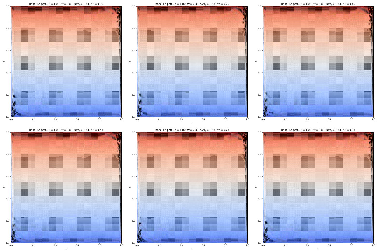
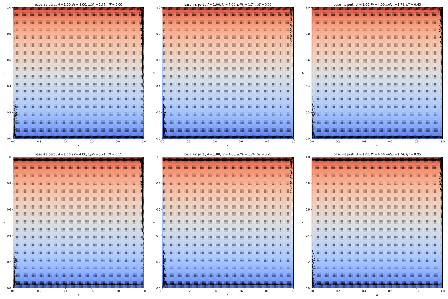
The base flows corresponding to regimes shown in figure 6 plus the perturbation at (a) $t=0$ and (b) $t=0.25T$. Arrows on streamlines indicate flow direction and colour represents temperature. Case VI is not shown since differences from case V are very small. For all cases I–VI, the same movies as referred to in figure 6 are represented online.

Movies of the unsteady states are provided as supplementary material available at https://doi.org/10.1017/jfm.2023.1056. The effects of varying aspect ratio $A$, along with the measured parameters $\omega /N_c$ and the regime diagram in the space set by $A$ and $Pr$, are discussed below.

3.2. Six unsteady regimes

The identification of the different regimes, shown in figure 6, is based on the detachment of the buoyancy current from the top and bottom boundaries and/or the location of the instability, the existence of a large-scale circulation and whether the scaled oscillation frequency is slow ($\omega /N_c \leq 1$) or fast ($\omega /N_c>1$), allowing for the presence of internal waves (or not). With increasing Prandtl number, the plumes detach earlier from the horizontal boundaries, and the presence of internal wave motions in the interior changes accordingly (see figure 6 I–VI); figure 7 I–V shows the transition from a convective regime with circulation cells moving locally through the tank to flows confined to boundary currents with horizontal exchange between them. Below we present each flow regime.

In case I ($Pr=0.1$) (see figure 6), there is no detachment of the buoyancy current from the horizontal boundaries and the hot buoyancy current joins the cold thermal boundary layer, resulting in a large cell circulation (see e.g. Xin & Le Quéré Reference Xin and Le Quéré2006), thus coupling the top and bottom motions. The phase plot (figure 6c I) shows a central rotary motion. In the perturbed flow (see figure 7a,b I) smaller cells move in the interior with the large cell circulation, showing that convective motions dominate. The oscillation frequency of this mode is larger than the buoyancy frequency, $\omega /N_c=2.26$, and internal waves can therefore not propagate. This flow regime is referred to as the fast cell circulation (FCc).

In case II ($Pr=0.35$) (see figure 6 II), the buoyancy current detaches from the boundary and meanders with a wavelength of approximately half the cavity width (figure 6a II). (Note that for the case $Pr=0.1$ shown above, an increase in width of the cavity would also result in a detachment of the buoyancy current.) This detachment causes the radiation of internal waves into the interior (see phase plots in figure 6c II) that have a dominant vertical mode with $\omega / N_c$ close to 1.0, leading to quasi vertical iso-phase lines. Vorticity perturbations (figure 6d II) show a maximum shear in the detached buoyancy current. The perturbed flow (figure 7a,b II) consists of two large cell structures with a dominant vertical transport, and large oscillations in the density profile, revealing the presence of internal waves. In contrast to the FCc case above, energy of the detached buoyancy currents is dispersed into internal wave motions such that the oscillation frequency is relatively small or ‘slow’. This regime is referred to as slow circulation cells (SCc).

In case III $Pr=0.53$ (see figure 6 III) the flow pattern changes from a convective flow to a horizontal exchange flow with a shift in direction at mid-height (figure 6a III). The buoyancy currents detach from the horizontal boundary close to the thermal wall. Oscillations are fast, $\omega /N_c>3$, and internal waves cannot propagate through the stratified interior, and the phase plot (figure 6c III) shows very different length scales in the buoyancy currents compared with those in the interior. In the absence of internal waves and a large-scale circulation, the top and bottom motions are decoupled. Thus, the independent growth of the unstable regions leads to different perturbation amplitudes, implying amplitude asymmetry (see figure 6b III). Because of the fast oscillations and the localisation of the instability in the corner regions, this flow is referred to as the fast corner flow (FCo).

In case IV $Pr=0.71$ (see figure 6 IV), we recover the case studied in detail in former studies (see e.g. Paolucci Reference Paolucci1990; Le Quéré & Behnia Reference Le Quéré and Behnia1998; Xin & Le Quéré Reference Xin and Le Quéré2006, and references therein), and more recently by Grayer et al. (Reference Grayer, Yalim, Welfert and Lopez2020). Here, $\omega / N_c \approx 0.5$, allowing for internal waves in the interior. These internal waves and the unstable corner regions are part of the same global instability mode (Xin & Le Quéré Reference Xin and Le Quéré2006) as the phase plot in figure 6(c IV) clearly shows. The amplitude of the internal waves in the interior is relatively weak compared with the amplitude in the corner regions. The perturbed base flow (figure 7a,b IV) shows next to the oscillating corner regions, recirculating regions in the interior that are slightly flattened by the internal buoyancy stratification. The absolute values of the perturbation amplitude of the top and bottom currents are identical or very close, which is referred to as symmetric in amplitude (not to be confused with centro-symmetry). The vorticity perturbations (figure 6d IV) have opposite signs at the top and bottom corners, revealing that this mode is anti-centro-symmetric (see the definition in § 3.1), which is the mode that appears for the lowest Rayleigh number, in agreement with Burroughs et al. (Reference Burroughs, Romero, Lehoucq and Salinger2004) and Oteski et al. (Reference Oteski, Duguet, Pastur and Le Quéré2015). The centro-symmetric mode appears for a slightly higher Rayleigh number.

In case V, $Pr=2.8$, the thermal boundary layer thickness is thin and the perturbation maxima are limited to very small corner regions (figure 6a–d V). The oscillation frequency is again increased (figure 6c V). Heat is diffused relatively slowly for this $Pr$ so that the temperature gradients near the top and bottom boundaries are larger than in the interior. The scaled oscillation frequency near the boundaries is $\omega /N \approx 0.8$ while in the interior $\omega /N \approx 1$, implying close to evanescent waves in the interior, as can be inferred from their almost vertical propagation direction (figure 6c V). The coupling between the top and bottom currents is therefore also weak, and there is amplitude symmetry only for some aspect ratios. In the interior, there is a smooth exchange flow (figure 7a,b V). This regime is referred to as fast corner flow with evanescent internal waves (FCoE).

In case VI, $Pr=4$, a simulation for a single aspect ratio has been conducted, showing that the oscillation frequency of the instability (here, $\omega /N_c \approx 1.8$) increases further with $Pr$ (see figure 6a–d VI). Internal waves emitted by the buoyancy currents near the top and bottom are evanescent and cannot propagate further into the interior. The two buoyancy currents have again different perturbation amplitudes and are therefore asymmetric in amplitude (figure 6b VI). The scales of motion in the boundary layer, top and bottom buoyancy currents as well as the interior are indeed very different (see figure 6c VI), showing two independent unstable regions. As will be shown below, this is a shear instability located at the wall. This regime is referred to as the fast instability at the wall (FW).

3.2.1. Corner and boundary layer flows

When zooming in the corner regions (figure 8) substantial flow changes can be noticed for different $Pr$. For $Pr=0.53$, the detachment and position of $L_h$ (see figure 1b) is small. Rolling vortex billows emerging from shear instability move to the corner (see supplementary movies) leading a maximum of the instability in the boundary layer near the corner (see figure 8a,e). For $Pr=0.71$, the instability has its maxima in the corner in the detached buoyancy current, where the main mixing occurs (see figure 8b,f). For $Pr=2.8$, the buoyancy current hardly detaches, and the flow is characterised by the presence of a downward jet close to the wall (at $0.98$ in figure 8c,g). The instability is located inside the detached buoyancy current and close to the boundary (figure 8g).

Figure 8.

Base flows showing close ups of the streamline–temperature fields of the corner regions for $A=1$ with maximum amplitude (a–d) for Prandtl numbers from 0.53 to 4.0, and (e–h) the corresponding amplitude fields. Note that zooms and aspect ratios in (a,b; e,f) and (c,d; g,h) are chosen differently for visualisation purposes.

For $Pr=4$, the boundary layer detaches right in the corner region where it also results in a downward return flow (figure 8d). The temperature gradient has its maximum very near to the wall. Outside the boundary layer, the strong shear between the upward boundary layer motion and the downward return flow with rotary motions similar to that for Kelvin–Helmholtz-type instabilities (see figure 8d,h and supplementary material) suggests a shear instability (see also Janssen & Henkes Reference Janssen and Henkes1995; Xu et al. Reference Xu, Patterson and Lei2008). In the interior, there is a horizontal exchange flow from right to left above mid-depth, and below from left to right (see figure 6 with $Pr \geq 0.53$). This exchange flow becomes dominant with increasing $Pr$.

The phase plots in figure 6(c) V–VI, ($Pr=2.8$ and $Pr=4.0$) show a large difference in scale between the boundary layers and the interior. Internal waves in the interior emerge from the buoyancy currents at the top and bottom boundaries, and are related to up- and downward motions of entrainment and detrainment, as shown in figure 8(c,d,g,h). Comparing these latter plots showing the perturbation amplitude (figure 8g,h), one notices that the downward flow for $Pr=4.0$ goes to mid-depth, and for $Pr=2.8$ to only approximately half that distance. In contrast to the case $Pr=2.8$, for $Pr=4$ the instability is located at the boundary where it has its maximum amplitude.

3.3. Instabilities and regime diagram

Figure 9(a) presents the normalised oscillation frequency of the leading linear mode with respect to $Pr$ for the four different values of $A$. Here, $N_c$ varies with $Pr$ (see figure 5) but the main variation is in $\omega$. The sharp jump at $Pr \approx 0.55 \pm 0.15$ separates two different regimes, one for small $Pr$ and one for large $Pr$, which can be deduced from scaling arguments (see Gill Reference Gill1966). From the stationary heat equation, one can deduce that the velocity along the boundary scales as $\kappa /\ell$ when $\ell$ is the length scale of the boundary layer. When introducing this scaling into the vorticity equation, with $\xi =\boldsymbol {\nabla } \times \boldsymbol {v_b}$, we obtain for the convective term $\boldsymbol {v_b} \boldsymbol{\cdot} \boldsymbol {\nabla } \xi \sim \kappa ^2 / \ell ^3$ and the diffusive term $\nu \nabla ^2 \xi \sim \nu \kappa / \ell ^3$. The ratio of the diffusive term over the convective term is equal to $Pr=\nu / \kappa$.

Figure 9.

(a) Maximum normalised oscillation frequency ($\omega /N_c$) and (b) regime diagram in space set by $Pr$ and aspect ratio $A$, with the colour indicating the logarithmic value of the normalised oscillation frequency $\omega /N_c$. Regime names are F for fast when $\omega /N_c>1$ and S for slow when $\omega /N_c<1$, $\blacksquare$ fast circulation cells (FCc); + slow circulation cells; $\blacktriangle$ fast corner flow (FCo); $\bigstar$ slow corner flow (SCo); + fast corner evanescent waves (FCoE), and $\blacklozenge$ fast instability at the wall (FW). (c) Diagram showing the symmetry index $I_{dif}$ (3.7), with the extremes (blue and red) corresponding to symmetric cases (anti-centro-symmetric – letter A – and centro-symmetric – letter C –) and yellow for amplitude asymmetry and no coupling between top and bottom regions.

For small Prandtl number the instability is thus convectively driven with large cell circulations (see also figure 7). In figure 9(a) ($Pr \lessapprox 0.5$) the flow is characterised by a cell circulation that is affected by the cavity aspect ratio $A$. For small cavity widths (large $A$), the buoyancy current remains attached to the horizontal boundary, and reinforces the motion in the thermal boundary layer at the wall, resulting in a fast motion with a high frequency of oscillation (see e.g. red squares in figure 5a). For large cavity widths (small $A$), the buoyancy currents detach from the horizontal boundaries, and radiate internal waves into the interior. The cell circulation is therefore weakened, resulting in a relatively slow motion with a low frequency of oscillation (see e.g. blue squares figure 5a), and thus a smaller $Pr$ is needed to increase $\omega /N_c$.

For large Prandtl numbers the diffusion term is larger than the convective term, from which it was concluded that the instability is buoyancy driven (see McBain, Armfield & Desrayaud Reference McBain, Armfield and Desrayaud2007). But the detrainment and entrainment motions and the related return flows that are due to these horizontal boundaries cannot be neglected. Janssen & Henkes (Reference Janssen and Henkes1995) (for different $Pr$ values, 0.25, 0.71 and 2) and Yahata (Reference Yahata1999) (for $Pr=0.71$) suggested this to be a shear instability with a change in instability from shear driven for $A >3.65$, to internal wave driven for $A<3.41$. For the present range in $Pr$ values, figure 9(a) shows strong variations around $Pr=0.55 \pm 0.15$ before the general trend to thinner boundaries and larger $\omega /N_c$ values for $Pr \gtrapprox 1$.

The regime diagram in figure 9(b) shows the oscillation frequency $\omega /N$ represented by the colour as a function of $Pr$ and aspect ratio $A$, with the symbols indicating the different regimes discussed above. For $Pr \lessapprox 0.5$, the above reasoning with a dominating cell-driven motion is represented in this diagram. But for $Pr > 0.5$, not less than 4 regimes appear due to the changing influences of internal waves (as indicated in figure 9(b) for $Pr>0.5$) and decreasing thickness of the boundary layer at the wall with $Pr$. In regime FCo there are no waves and no coupling; in SCo for the majority of cases there are waves and the top and bottom regions couple. For even larger $Pr$ values internal waves weaken, and the thermal boundary layers are thinner (FCoE). For $Pr = 4.0$ (regime FW) there are no waves and no coupling. In contrast to the regime FCo, the instability occurs at the boundary. Since for larger $Pr$ the lateral boundary layers will be even closer to the walls, one may speculate that this regime will not further change. Simulations were tested for aspect ratio, $A=6$ and $Pr=0.7$ as in Xin & Le Quéré (Reference Xin and Le Quéré2006), showing again the FCc regime. In view of the mentioned increase of the boundary layer thickness with height, and the increasing inertia of the buoyancy current for taller cavities and thus larger $L_h$, the regime FCo most likely disappears for larger aspect ratio $A$.

Figure 9(c) shows the amplitude asymmetry according to the definition of (3.7) as a function of $Pr$ and $A$. In the FCo regime, due to the absence of internal waves and cell circulation, the flow is asymmetric in amplitude. For larger $Pr$ (regime SCo), waves are present, and generally (except for $A=1$, $Pr=1.4$) couple the top and bottom regions. Not all flows with internal waves are found to be symmetric in amplitude. Wave patterns in the interior vary considerably depending on the aspect ratio of the cavity and the location of the detachment of the buoyancy currents, and some do not allow for coupling. This may explain the isolated points of asymmetry in amplitude (orange, green and yellow) for regimes with internal waves (SCc, SCo in figure 9b). In the regime FCoE ($Pr = 2.8$), internal waves are close to evanescent, so that the coupling is generally weak in this regime, causing asymmetry in the amplitude for most cases, and complete asymmetry in the regime FW ($Pr=4$). Regime FCc is symmetric in amplitude due to the coupling by the cell circulation, and SCc due to internal waves except for one case ($A=1$ and $Pr=0.2$). For $Pr \gtrapprox 0.5$, the cell circulation was found to increase in strength for larger aspect ratios $A>1$, and appeared to cause amplitude symmetry also in the regime FCo, thus showing some overlap between the regimes (dashed line in figure 9b,c). This suggest that, for higher aspect ratios $A \geq 2$ and $Pr < 0.6$, the flow is also dominated by convectively driven cells.

Figure 9(c) also shows anti-centro- and centro-symmetry (letters A and C, respectively). These results are coherent with former results (see e.g. Burroughs et al. Reference Burroughs, Romero, Lehoucq and Salinger2004; Xin & Le Quéré Reference Xin and Le Quéré2006; Oteski et al. Reference Oteski, Duguet, Pastur and Le Quéré2015). However, no systematic variation with the regime diagram and amplitude asymmetry was found in this context. It is expected that more pertinent results could be found with a continuous parameter variation method (see e.g. Lyubimova et al. Reference Lyubimova, Lyubimov, Morozov, Scuridin, Hadid and Henry2009). This is left open for further research.

Figure 9(a,b) suggests that there is a transition in instability in the regime $Pr =0.55 \pm 0.15$. The increase of both the shear and the density gradient between the detached buoyancy currents and the motion in the boundary layer with $Pr$, make it hard, however, to determine when exactly the instability is buoyancy or shear driven. A quantitative comparison is needed to determine the precise nature of the instability for each $Pr$. This is undertaken in a separate study.

Outside the space of this regime diagram, for aspect ratios greater than 3 or 4, the boundary layer will become unstable with, for large $Ra$, the detachment of vortices disturbing the internal stratification and generating internal waves (Xin & Le Quéré Reference Xin and Le Quéré1995). In the limit of very large $Pr$ and large $A$, the onset of local cells was found in the core, the number of cells being set by the scale of the instability in the boundary layer (see Daniels Reference Daniels1985, Reference Daniels1987, and references therein).

Figure 10(a,b) shows the variation of the critical Rayleigh number and Reynolds number as a function of $Pr$, respectively. There is a clear transition between the two regimes, with $Ra_c \sim Pr^2$ for $Pr<1$ and $Ra_c\sim Pr^5$ for $Pr>1$. In between (i.e. for $0.5< Pr \lessapprox 2$) there is an intermediate region where internal waves are present and play a role in the dynamics. In both figures 10(a) and 10(b), for $Pr>1$ the aspect ratio does not affect the results. Finally, it is noteworthy that the Reynolds number defined as $Re_c=Ra_c^{0.5}/Pr$ could serve as an appropriate critical value for the onset of instability since it varies just between $(2\pm 1) 10^4$ for $Pr<1$, and for $Pr>1$, $Re_c=10^4 Pr^2$, whereas the Rayleigh number varies over six decades (see figure 10b). This Reynolds number compares well with a Reynolds number based on the maximum velocity in the cavity and the appropriate typical length scale.

Figure 10.

Critical Rayleigh number as a function of Prandtl number and (b) the Reynolds number derived from the critical Rayleigh number and Prandtl number against Prandtl number for different aspect ratios $A$ (see legend). The dashed lines represent the power laws discussed in the text.