1. INTRODUCTION
Inertial Navigation Systems (INS) are widely adopted for their autonomous navigation ability. However, the navigation error will accumulate with time due to the integration working principle (Wang and Gao, Reference Wang and Gao2010). Two important features of ocean vehicle navigation are requirements for long operational durations and high accuracy. Therefore, the disadvantage of an INS will become obvious in a short period. To counter this, INS are frequently aided with external information to eliminate error drift.
The common existing methods for marine INS include gyrocompass and filters, integrating Doppler Velocity Log (DVL) (Xu et al., Reference Xu, Liu, Shan, Zhang and Wang2014) or Global Navigation Satellite Systems (GNSS) (most commonly the Global Positioning System (GPS)) with INS (Hwang et al., Reference Hwang, Sang, Sang, Park and Rizos2005). The major drawback of these methods is the dependence on external information. The availability of accurate and secure external information cannot be guaranteed. GNSS signals can suffer from outages (Atia et al., Reference Atia, Noureldin and Korenberg2011), signal blockage and are susceptible to be disruption by jamming and spoofing (Wang et al., Reference Wang, Diao, Gao, Zhu and Xiao2015). DVL is an independent velocity measuring equipment commonly used on ships (Xu et al., Reference Xu, Liu, Shan, Zhang and Wang2014; Gao et al., Reference Gao, Li, Zhou and Li2014). However, environment factors have a direct impact on DVL measurement accuracy. These defects pose challenges to ocean vehicle navigation with the existing external information aided solutions.
To overcome the drawback of external information aided solutions, navigation methods based on Artificial Intelligence (AI) have been suggested to overcome the inadequacies of the common existing methods (Chen and Fang, Reference Chen and Fang2014; Noureldin et al., Reference Noureldin, El-Shafie and Bayoumi2011; Chen et al., Reference Chen, Shen, Zhang, Tomizuka, Xu and Chiu2013). The essential pre-trained model of the AI-based method operates in prediction mode to correct INS errors in the case of external information outages. The model is obtained through a large amount of computation and sample data ranges, and it should be retrained if there are changes in the operating conditions. The real-time application is hard to achieve, and it cannot cope with the situation of long external information outages.
These limitations motivated research to investigate alternative methods, predominantly on the methods with aiding of the vehicle dynamic knowledge. The dynamic constraint methods have been applied in land vehicle navigation (Wang and Gao, Reference Wang and Gao2010; Dissanayake et al., Reference Dissanayake, Sukkarieh, Nebot and Durrant-Whyte2001; Wang et al., Reference Wang, Gao and Zhang2005). The idea behind the approach is to derive additional observations from dynamic knowledge, which are utilised to curb the stand-alone INS navigation divergence. For instance, the changes of velocity and angular rate are assumed to be zero in the stationary condition, and no significant motion acceleration along the transverse direction exists when moving along a straight track (Wang and Gao, Reference Wang and Gao2010). In Wang and Gao (Reference Wang and Gao2010), typical dynamic conditions are firstly defined by combining analysis of inertial data and a fuzzy expert system, and then the dynamic aiding data is applied to update a Kalman Filter (KF) when GPS is unavailable.
To further improve the performance of an ocean vehicle navigation system, the utilisation of two ocean vehicle dynamic constraints are proposed to aid the inertial navigation. Differing from a land vehicle, constant speed cruise and quasi-static modes are the typical dynamics. In this paper, the quasi-static condition refers to when an ocean vehicle is in the anchored condition or moored condition. There is wave motion along the waves and almost no displacement. We derive additional velocity and position observations separately in these two conditions and apply them to update the KF. More importantly, before applying the observations properly, the dynamic conditions should be identified accurately. In this paper, we firstly select the accelerometer and gyroscope measurement-related features and then accomplish identification through a multiple-layer strategy by using the selected features. To some extent, the INS character of independence from external support can be enhanced by the proposed method. Simulation and experiment results show that the proposed method can maintain high attitude accuracy even when external information is missing for a long period.
2. ADDITIONAL DYNAMICALLY-DERIVED OBSERVATIONS
2.1. Dynamic constraints
Ocean vehicles are in the condition of constant speed cruise or moored for a great part of time. In a constant speed cruise condition, the ocean vehicle sails on a fixed heading at a constant speed. In this condition, unchanged velocity and heading are distinguishing features. The traditional navigation equations can be simplified as follows:
 $$\dot{V}=0$$
 $$\dot{\phi}_u=0$$
where V is the vehicle velocity, ϕ u is the heading. Equations (1) and (2) indicate unchanged velocity and heading. When the ocean vehicle remains moored, the most obvious feature is the unchanged position. The velocity is disturbed by the wave motion and does not remain at zero. Thus, it is nearly static, and in this paper, we define the condition as a quasi-static condition. The dynamic constraint can be expressed as Equation (3):
 $$\dot{P}=0$$
where P is the position. Thus, at these two specific conditions, it is possible to directly obtain velocity and position information without any external support equipment.
2.2. Dynamic-derived observations and error analysis
2.2.1. Constant speed cruise condition
When the vehicle moves at a constant speed on a fixed heading, the velocity is an effective observation to correct the attitude error. If it is detected that the vehicle is in the constant speed cruise condition, the current velocity can be used as a useful observation.
 $$V_{obs}=V(t_N)$$
where V(t N) is the velocity measurement at the current time t N, V obs is the velocity observation. The accuracy of the current velocity is a key factor affecting the estimation accuracy of filters. For an ocean vehicle, the heading error has a common relationship with the velocity error which according to the Octans user guide (iXblue, 2008), can be expressed in Equation (5):
 $$\delta\phi_u =\displaystyle{{\delta V_N}\over{5\pi}}\hbox{sec}\,L$$
where δϕ u is the heading error, δV N is the equivalent north velocity error and L is the latitude. Take an INS with accelerometer bias 50 μg (1σ) and gyroscope bias 0·01°/h (1σ) for example. Without external information for one hour, the accumulated velocity error is only approximately 1 m/s and will lead to a heading error δϕ u of about 0·1° sec L. This demonstrates that the current velocity obtained in this condition is acceptable to be used as the observation.
2.2.2. Quasi-static condition
The direct observation during the moored condition is the unchanged position:
 $$P_{obs}=P(t_N)$$
where P(t N) is position at the current time t N and P obs is the position observation. For an ocean vehicle, the moored condition is an approximately static condition due to the wave effect. So, in this paper, it is defined as a quasi-static condition. In this condition, the velocity is variable and cannot be predicted. However, the position is limited in a range. For an INS with accelerometer bias 50 μg (1σ) and gyroscope bias 0·01°/h (1σ), the position error of the pure inertial navigation algorithm is about 1 nautical mile for one hour, namely 1 minute of arc angular position error. The position error is acceptable to the INS requiring 1° sec L heading accuracy. Therefore, the position is adopted as the observation.
3. DYNAMIC IDENTIFICATION
The dynamic conditions should be identified accurately before applying the obtained observations. In practical applications, the inertial sensor output will be contaminated by noise and affected by the operating environment factors, as described in the last section. Therefore, the identification process of dynamic conditions is carried out with the capability of dealing with the effect of the above factors.
The quasi-static condition can be considered as a special case of the constant speed cruise. Therefore, the identification consists of two steps. Firstly, it is judged whether it satisfies the requirements of constant speed cruise. If it satisfies, a further judgement is taken to conduct the quasi-static identification. The specific identification criteria follow.
3.1. Constant speed cruise condition identification
We denote the body frame by b, the navigation frame by n, the inertial frame by i and the Earth frame by e. When the vehicle moves on a constant heading, the vertical angular rate is very small. Further, if the speed is kept constant, the horizontal acceleration is approximately zero. Thus, the judgment includes two parts: vertical angular rate and horizontal acceleration.
(1)
 $\vert \omega^{b}_{nbz}\lpar t_{N}\rpar \vert <\varepsilon_{1}$
(2)
$\vert \bar{f}^{b}_{x}\lpar t_{N}\rpar \vert <\varepsilon_{2}$ and $\vert \bar{f}^{b}_{y}\lpar t_{N}\rpar \vert <\varepsilon_{2}$
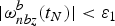
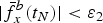
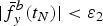
where  $\omega^{b}_{nbz}$ is the vertical angular rate measured in the body frame at the current time t N,
 $\vert \bar{f}^{b}_{x}\lpar t_{N}\rpar \vert $ and
 $\vert \bar{f}^{b}_{y}\lpar t_{N}\rpar \vert $ are the averages of the horizontal acceleration during a time interval until t N; here we set the time interval as one minute. ε1 and ε2 are corresponding thresholds.
Compared with the vertical angular rate caused by vehicle motion, the effect of noise on the raw gyroscope measurement is small and the raw gyroscope measurement is used directly in the judgment. In contrast, the quantised noise of the raw accelerometer measurement is relatively large. So, the averages of the horizontal acceleration are used in the judgment. The thresholds are set according to the precision level of the INS and the operating environment. For example, ε1 and ε2 will be set as 0·005 rad/s and 0·1 m/s2 for the INS with accelerometer bias 50 μg (1σ) and gyroscope bias is 0·01°/h (1σ) in the common operating environment.
3.2. Quasi-static condition identification
When the accelerometer and gyroscope measurements satisfy the constant speed cruise condition, a further quasi-static judgment will be taken. When an ocean vehicle remains moored, the acceleration of the vehicle changes, and is different from the moving condition. Thus, the difference of the averages of the horizontal acceleration in one minute is used in this step. The further criterion is:
(3)
$\vert d\_f^{b}_{x}\lpar t_{N}\rpar \vert <\varepsilon_{3}$ and $\vert d\_f^{b}_{y}\lpar t_{N}\rpar \vert <\varepsilon_{3}$

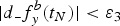
where
 $$\eqalign{& d\_f_x^b (t_N) = \bar f_x^b (t_N) - \bar f_x^b (t_N - n) \cr & d\_f_y^b (t_N) = \bar f_y^b (t_N) - \bar f_y^b (t_N - n)} $$
where  $\bar{f}^{b}_{x}\lpar t_{N}\rpar $ and
 $\bar{f}^{b}_{y}\lpar t_{N}\rpar $ are the averages of the horizontal acceleration in one minute until t N.
 $\bar{f}^{b}_{x}\lpar t_{N}-n\rpar $ and
 $\bar{f}^{b}_{y}\lpar t_{N}-n\rpar $ are the averages in the last minute. ε3 will be set as 0·002 m/s2 for the INS with accelerometer bias 50 μg (1σ) and gyroscope bias is 0·01°/h (1σ) for the common operating environment.
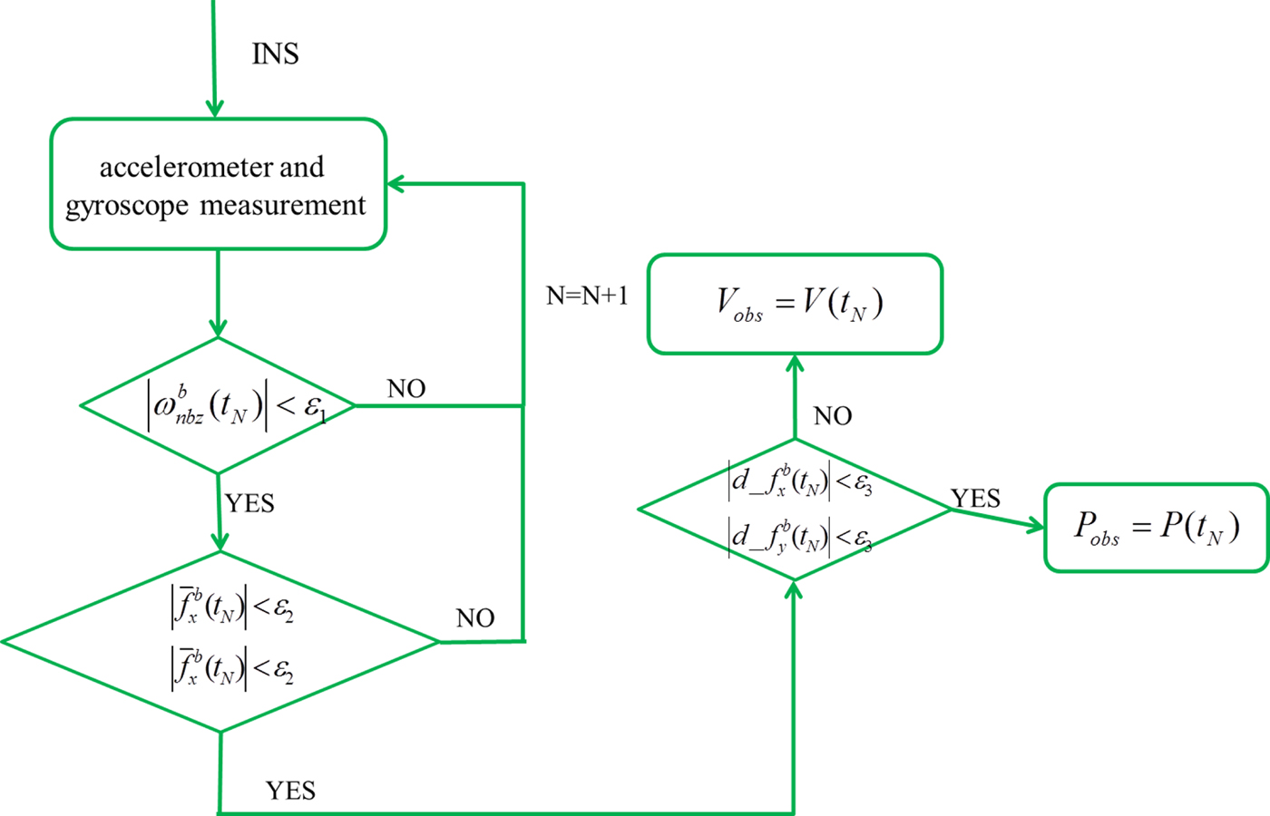
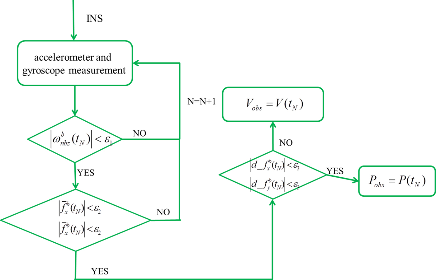
The whole identification process is shown in Figure 1. At the end of the process, if  $d\_f_{x}^{b} \lpar t_{N}\rpar $ and
 $d\_f_{y}^{b} \lpar t_{N}\rpar $ satisfy the criteria, the vehicle is in a quasi-static condition and the position information is used as the observation; if not, the vehicle is in constant speed cruise, and the velocity information is used as the observation.
Flowchart of the identification process.
4. DESIGN OF THE NAVIGATION FILTER
With the dynamically-aided observations, a Kalman Filter (KF) is designed to estimate the inertial sensor error and navigation error. In this paper, the derived observations are only available in velocity and position and the design of the filter aims to obtain high attitude accuracy. The system and measurement models are designed as follows.
4.1. System model
For an ocean vehicle, the systemic error equations are developed in the navigation n-frame. We chose angular position error δθ x, δθ y horizontal velocity error δ V x, δ V y, attitude (pitch, roll, heading) error ψx, ψy, ψz, gyroscope bias εx, εy, εz, and accelerometer bias ∇x, ∇y as the state vector X. They are all expressed in the n-frame. The system error equations can be expressed in this frame as follows:
 $$\matrix{ X \hfill & { = \left[ {\matrix{ {\delta \theta _x} & {\delta \theta _y} & {\delta V_x} & {\delta V_y} & {\psi _x} & {\psi _y} & {\psi _z} & {\varepsilon _x} & {\varepsilon _y} & {\varepsilon _z} & {\nabla _x} & {\nabla _y} \cr } } \right]} \hfill \cr {} \hfill & {\left\{ {\matrix{ {\delta {\dot \theta }_x = - \displaystyle{{v_z} \over R}\delta \theta _x - \displaystyle{1 \over R}\delta V_y} \hfill \cr {\delta {\dot \theta }_y = - \displaystyle{{v_z} \over R}\delta \theta _y - \displaystyle{1 \over R}\delta V_x} \hfill \cr {\delta {\dot V}_x = - g\delta \theta _y + 2\omega _{iez}^n \delta V_y - f_z\psi _y + f_y\psi _z + \nabla _x} \hfill \cr {\delta {\dot V}_y = g\delta \theta _x - 2\omega _{iez}^n \delta V_x + f_z\psi _x - f_x\psi _z + \nabla _y} \hfill \cr {{\dot \psi }_x = \omega _{iez}^n \psi _y - \omega _{iny}^n \psi _z - \varepsilon _x} \hfill \cr {{\dot \psi }_y = - \omega _{iez}^n \psi _y + \omega _{inx}^n \psi _z - \varepsilon _y} \hfill \cr {{\dot \psi }_z = \omega _{iny}^n \psi _x - \omega _{inx}^n \psi _y - \varepsilon _z} \hfill \cr {\varepsilon _x = C_{11}\varepsilon _x^b + C_{12}\varepsilon _y^b + C_{13}\varepsilon _z^b } \hfill \cr {\varepsilon _y = C_{21}\varepsilon _x^b + C_{22}\varepsilon _y^b + C_{23}\varepsilon _z^b } \hfill \cr {\varepsilon _z = C_{31}\varepsilon _x^b + C_{32}\varepsilon _y^b + C_{33}\varepsilon _z^b } \hfill \cr {\nabla _x = C_{11}\nabla _x^b + C_{12}\nabla _y^b } \hfill \cr {\nabla _y = C_{21}\nabla _x^b + C_{22}\nabla _y^b } \hfill \cr } } \right.} \hfill \cr } $$
where f is the accelerometer output in the n-frame, R is the earth radius,  $\omega^{n}_{ie}$ is the Earth rotation rate and
 $\omega^{n}_{in}$ is the rotation rate of the i-frame with respect to the b-frame expressed in the n-frame. C ij is the element of
 $C_{b}^{n}$ in the j-th column of the i-th row.
 $C^{n}_{b}$ is the direction cosine matrix representing the rotation from the b-frame to the n-frame.
4.2. Measurement model
Dynamically-derived measurements were discussed in the last section. The corresponding measurement models for the constant speed cruise condition and the quasi-static condition are now given.
In the constant speed cruise condition, the velocity observation is available. The measurement is given as
 $$\matrix{ {Z_1} \hfill & { = V_{INS} - V_{obs}} \hfill \cr {} \hfill & { = \left[ {\matrix{ 1 & 0 \cr 0 & 1 \cr } } \right]\left[ {\matrix{ {\delta V_x} \cr {\delta V_y} \cr } } \right]} \hfill \cr } $$
where V INS is the velocity calculated by the INS.
In the quasi-static condition, the available observation is the position information. The corresponding measurement is given as
 $$Z_2 = \left[ {\matrix{ {C_{23}} \cr {C_{31}} \cr } } \right] = \left[ {\matrix{ 1 & 0 \cr 0 & 1 \cr } } \right]\left[ {\matrix{ {\delta \theta _x} \cr {\delta \theta _y} \cr } } \right]$$
where
 $$C=\bar{C}^n_eC^e_n$$
 $$\bar C_e^n = [I - (\delta \theta \times )]C_e^n = \left[ {\matrix{ 1 & {\delta \theta _z} & { - \delta \theta _y} \cr { - \delta \theta _z} & 1 & {\delta \theta _x} \cr {\delta \theta _y} & { - \delta \theta _x} & 1 \cr } } \right]C_e^n $$
where  $C^{n}_{e}$ is the position matrix and the direction cosine matrix representing the rotation from the e-frame to the n-frame.
 $\bar{C}^{n}_{e}$ is the corresponding corrected matrix. For an ocean vehicle, the angular position error δθ x, δθ y, δθ z will be at the level of minute of arc even over one hour. So, the angular position error is considered as a small quantity.
5. SIMULATION AND EXPERIMENT
In order to evaluate the availability of the dynamic identification and the accuracy of the dynamically-aided Kalman filter method, both simulation and experiment are carried out in this section. To further validate its performance, the dynamically-aided Kalman filter method is compared with the pure inertial navigation method and GPS/INS integration method. In this section, we call the proposed method the dynamically-aided method.
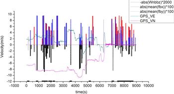
For the result presentations, if the condition satisfies the identification criteria, the identification parameters will multiply a constant K. This aims to amplify the inertial senor output to the same magnitude as the GPS information, to show the results more directly. The value will be set to zero when the identification criteria are not satisfied.
5.1. Simulation
A trajectory of an ocean vehicle is simulated for 15,000 s. It includes a wharf start for 300 s, accelerating to 12 m/s over 30 s, constant speed cruise 14,340 s, decelerating to 0 m/s over 30 s and then remaining moored for 300 s. The inertial sensor error parameters of the INS are:
1) Gyroscope bias 0·01°/h, scale factor 50 parts per million (ppm), misalignment error 30 arc seconds (Asec) noise 0·005°/h/
$\sqrt{Hz}$;2) accelerometer bias 50 μg, scale factor 50 ppm, misalignment error 30 Asec, noise 20 μg/
$\sqrt{Hz}$.


The main objective of the simulation is to evaluate how much the attitude accuracy can be improved by the proposed method under both constant speed cruise and quasi-static conditions. Equivalent noise is set to simulate the impact of sea factors on the Inertial Measurement Unit (IMU).
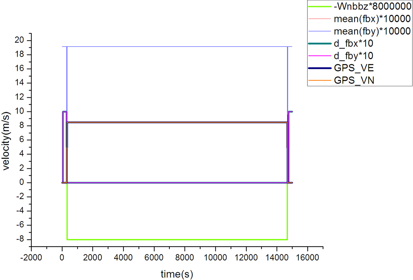
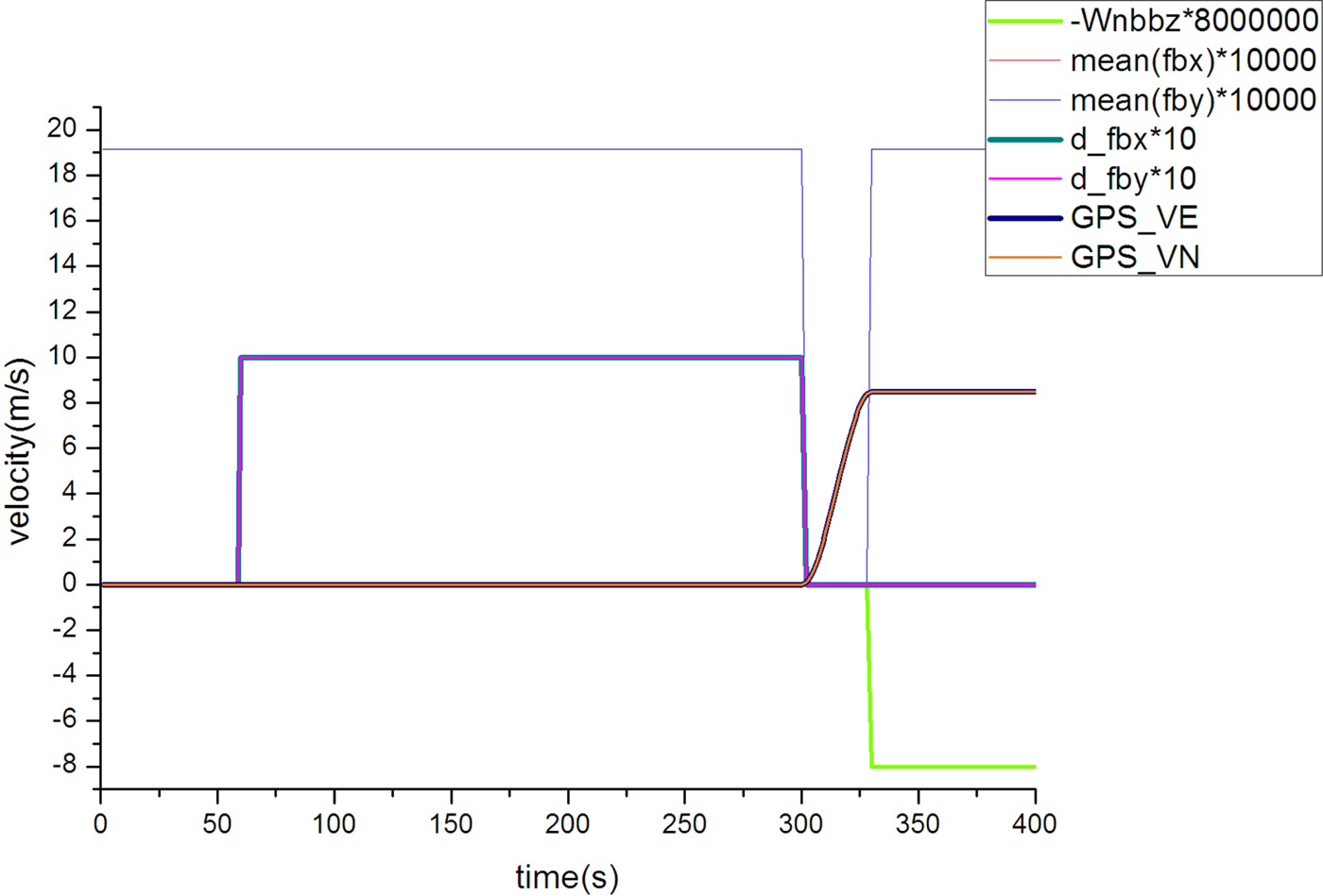
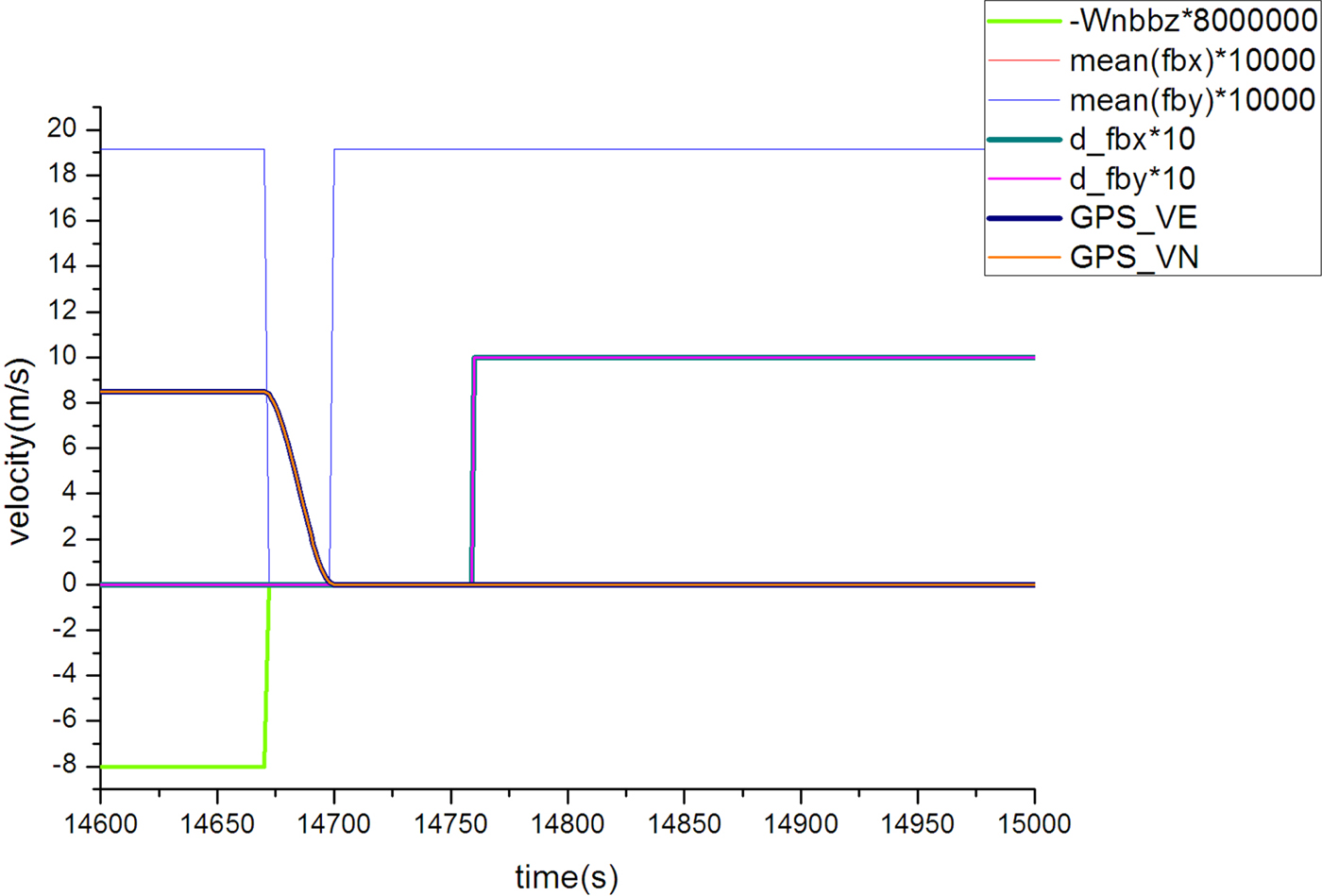
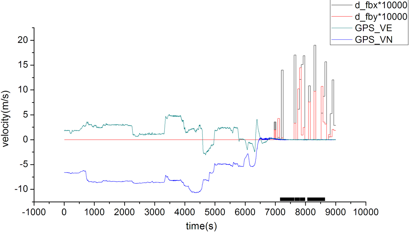
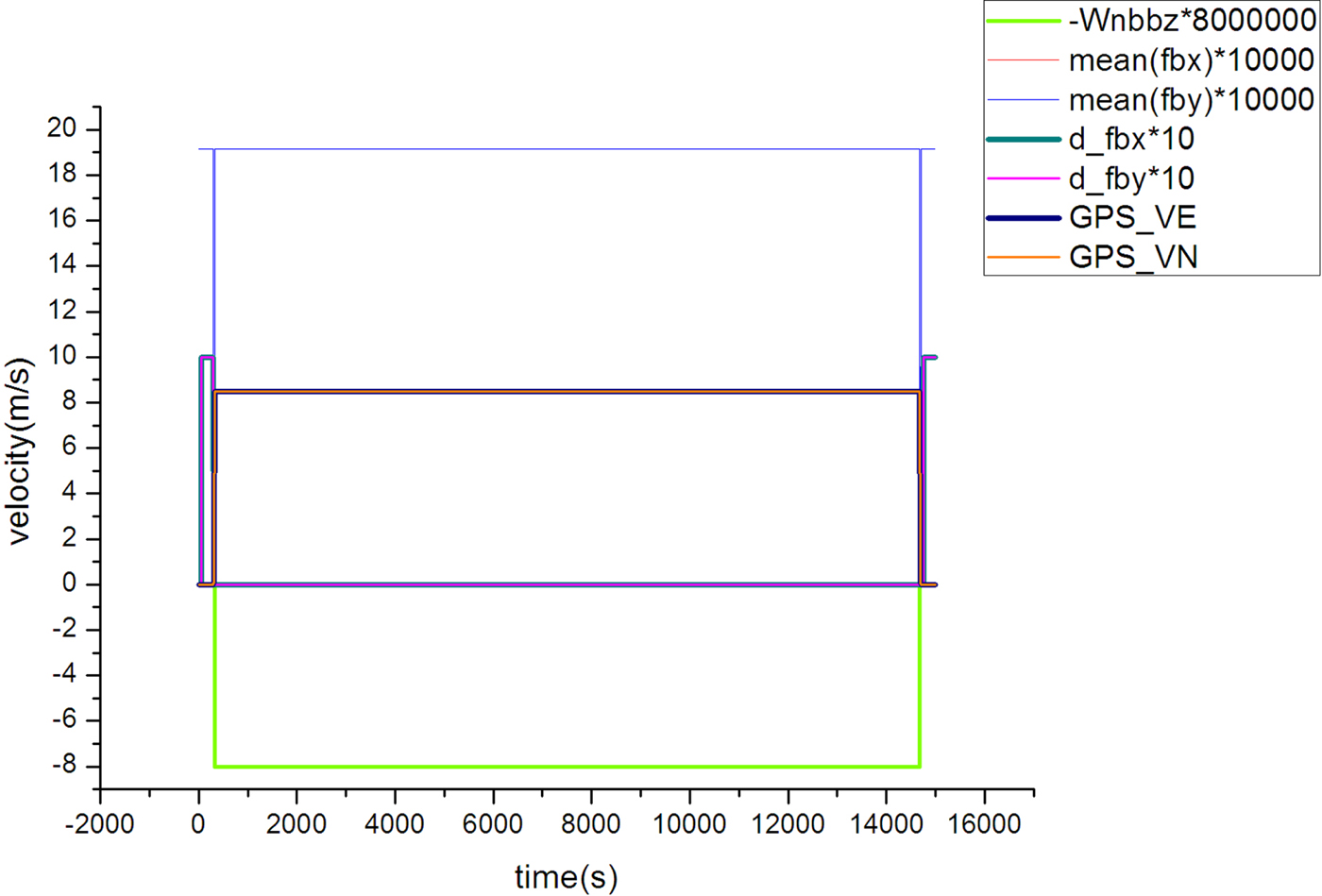
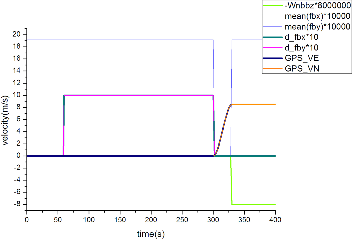
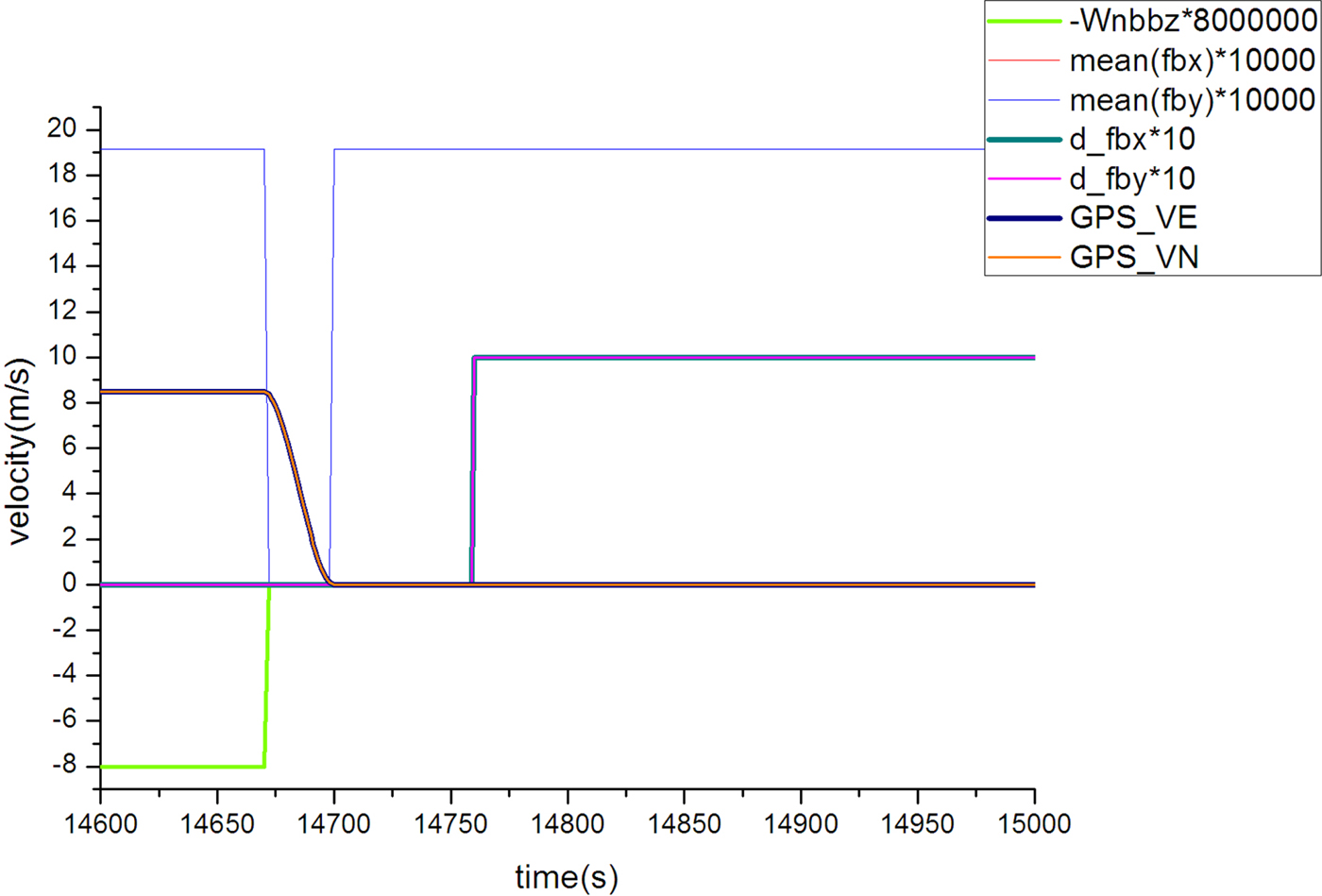
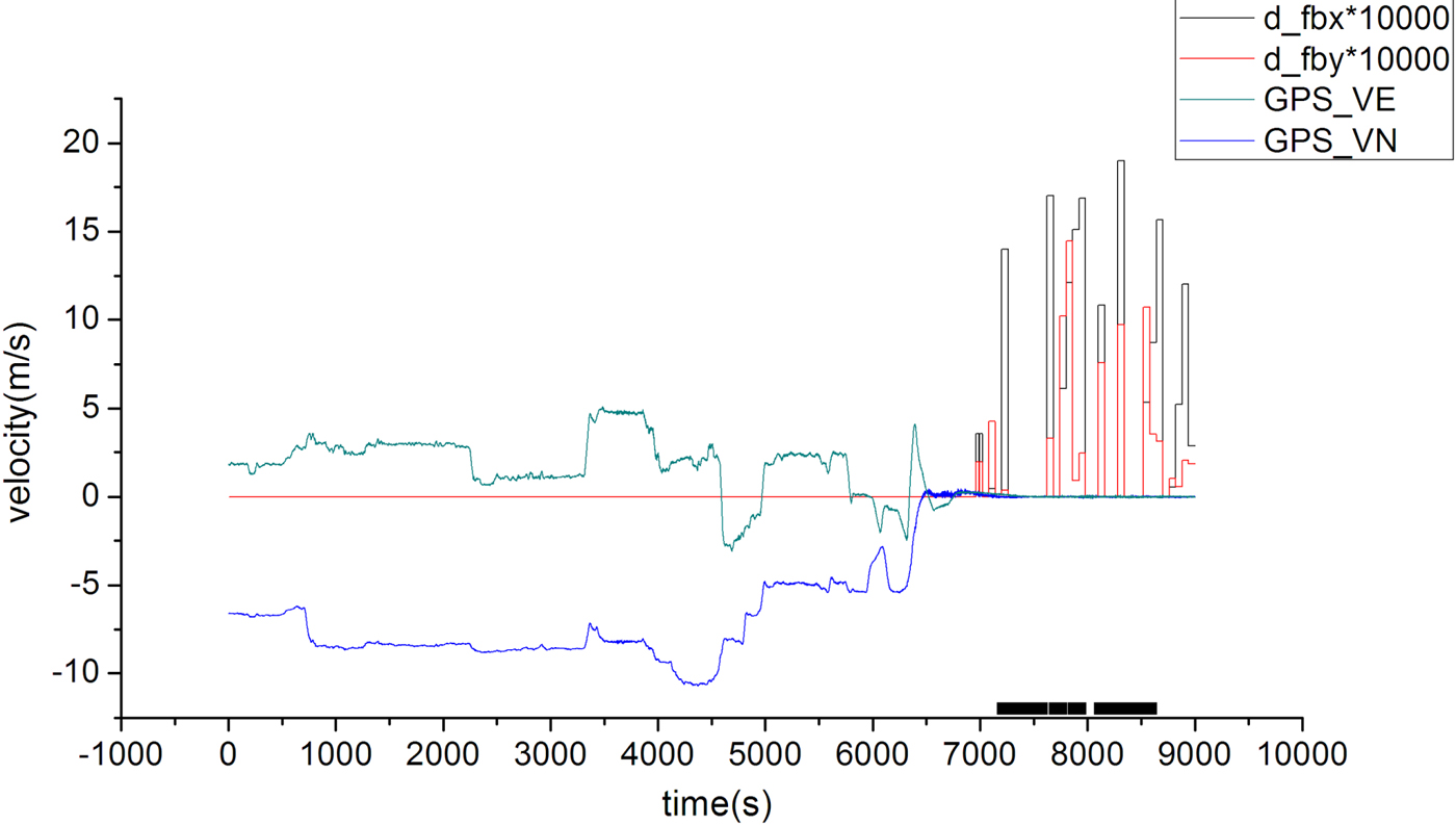
Firstly, the dynamic identification method is evaluated. Figures 2–4 show the dynamic identification results. Both the GPS reference velocity and related identification parameters are listed in the figures. GPS_VE and GPS_VN are the east and north velocity provided by GPS; Wnbbz represents  $\omega_{nbz}^{b}$, the vertical angular rate; mean(fbx) and mean(fby) are
 $\bar{f}^{b}_{x}\lpar t_{N}\rpar $ and
 $\bar{f}^{b}_{y}\lpar t_{N}\rpar $, the averages of the horizontal acceleration. d_fbx and d_fby represent the difference of acceleration averages,
 $d\_f_{x}^{b} \lpar t_{N}\rpar $ and
 $d\_f_{y}^{b} \lpar t_{N}\rpar $.
Identification results during the whole trajectory.
Identification results in the first 400 s.
Identification results in the last 400 s.
It should be mentioned that in the simulation, the operating environmental factors are not easy to simulate well.  $d\_f_{x}^{b} \lpar t_{N}\rpar $ and
 $d\_f_{y}^{b} \lpar t_{N}\rpar $ are zero in the moored condition due to the simulation limitation. In order to show the identification result, when the condition is identified as quasi-static,
 $d\_f_{x}^{b} \lpar t_{N}\rpar $ and
 $d\_f_{y}^{b} \lpar t_{N}\rpar $ are set to one.
By comparing the identified conditions with the reference information provided by GPS, it is verified that the constant speed cruise condition and quasi-static condition are correctly identified. When the GPS reference velocity is relatively steady, it indicates that the ocean vehicle is at a constant velocity in a straight line. In this case, it can be seen from Figure 2 that the constant speed cruise is correctly identified. In Figure 3, the period of the first 55 ~ 300 s is identified as the quasi-static condition; and in Figure 4, the period of the last 14, 760 ~ 15, 000 s is also correctly identified.
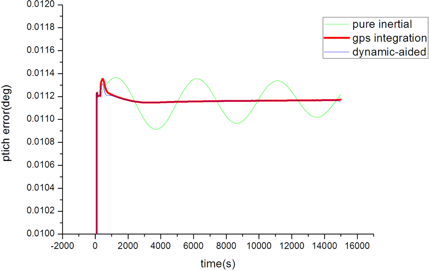
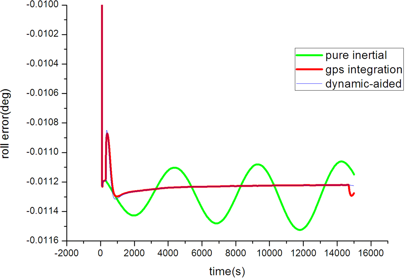
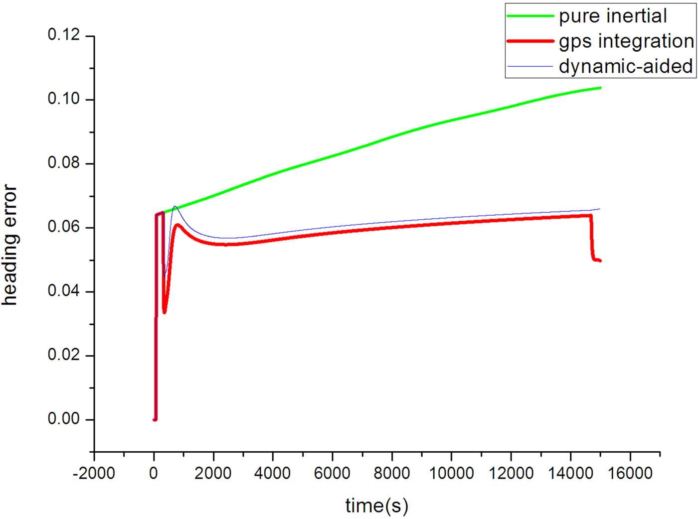
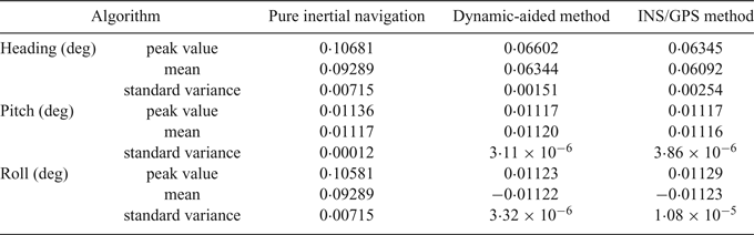
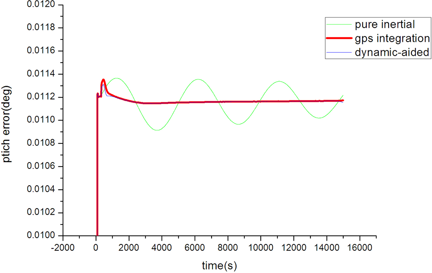
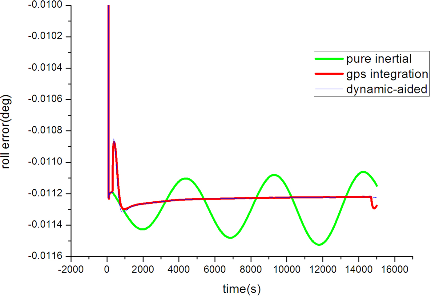
The attitude errors of the proposed method, the pure inertial navigation method and GPS/INS integration method are shown in Figures 5–7. It can be seen that the pitch and roll estimation of the proposed method are more accurate than the pure inertial navigation method, and the accuracy is close to that of the GPS integration method. For the heading performance, the error of the pure inertial navigation method is 0·106°; however, the error of the proposed method is only 0·066°. Table 1 summarises the attitude error peak value, after the filter comes to the steady state, and the mean and standard variance. In summary, the dynamically-aided observations enable the stand-alone INS to limit the attitude error.
Pitch error.
Roll error.
Heading error.
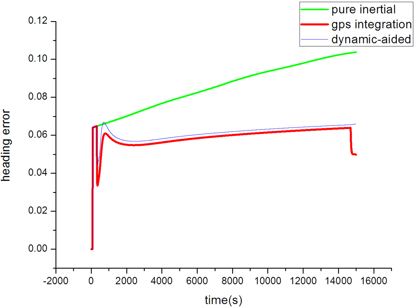
Attitude estimation in the simulation.

5.2. Experiment
The sea experiment on a 10,000 tonne ocean-going ship includes various working conditions according to the motion path, including constant speed and turning manoeuvres. The test trajectory includes about 7,000 s sailing, followed by 2,000 s remaining moored. In the experiment, an INS with 50 μg accelerometer bias and a 0·02°/h fibre-optic gyroscope bias was chosen to evaluate the performance of the algorithm. The sample rate of GPS was 1 Hz, position accuracy 10 m and velocity accuracy 0·1 m/s. The INS was fixed at the mass centre of the ship. The sample rate of INS was 100 Hz and the GPS receiver was fixed into the INS. The GPS antenna was mounted above the ship's bridge. The lever arm between GPS and INS was measured and compensated. The INS and GPS data were calculated after time synchronisation. Using GPS-assisted inertial navigation as a reference, we made a comparison between the proposed method and pure inertial navigation.
The experimental results give the same results for the data processing method in the simulation when testing the dynamic identification algorithm. In Figures 8 and 9 the identified time windows are highlighted on the time axis. Figure 8 shows constant speed cruise identification results. It can be seen that when GPS_VE and GPS_VN were relatively steady, the related parameters were not zero and the constant speed cruise condition was identified. The velocity could thus be used as the filter observation. Figure 9 shows the quasi-static condition identification results. In the last 2,000 s, d_fbx and d_fby were not zero and the quasi-static condition was successfully identified. At this time, the position information is used as the observation.
Constant speed cruise identification during whole trajectory.
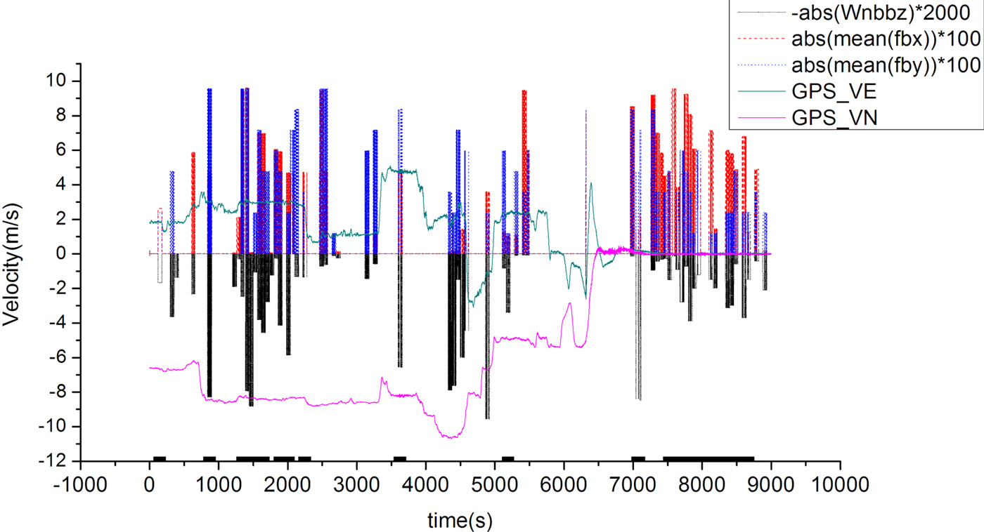
Quasi-static condition identification during whole trajectory.
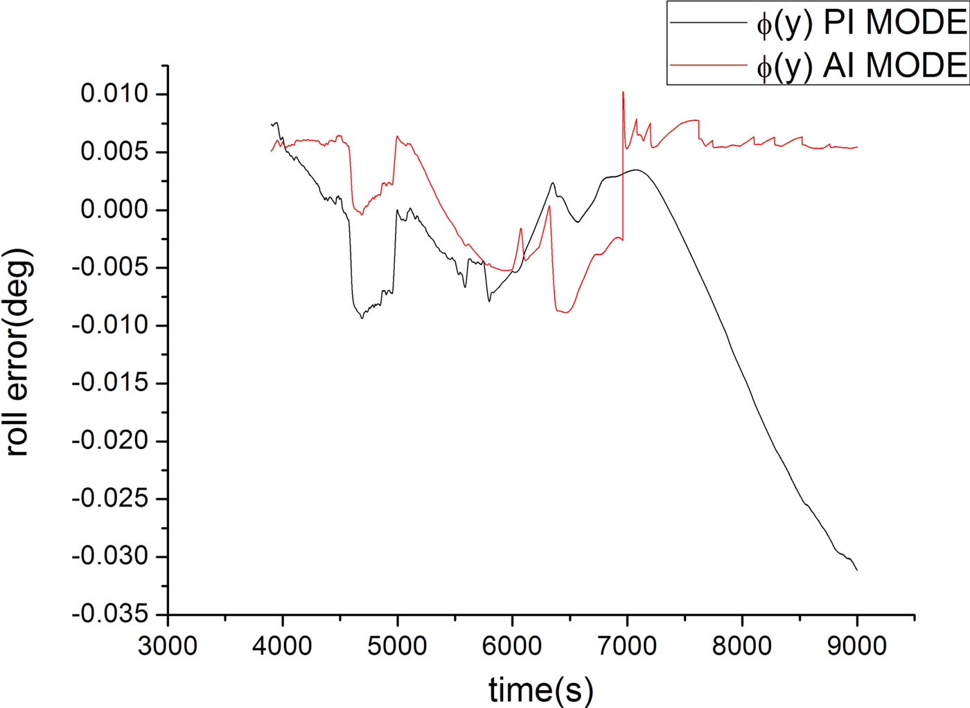
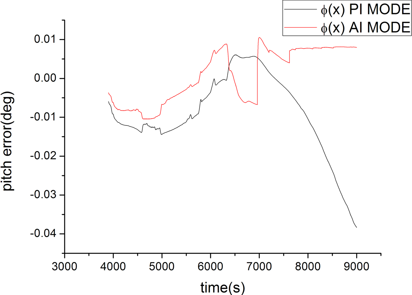
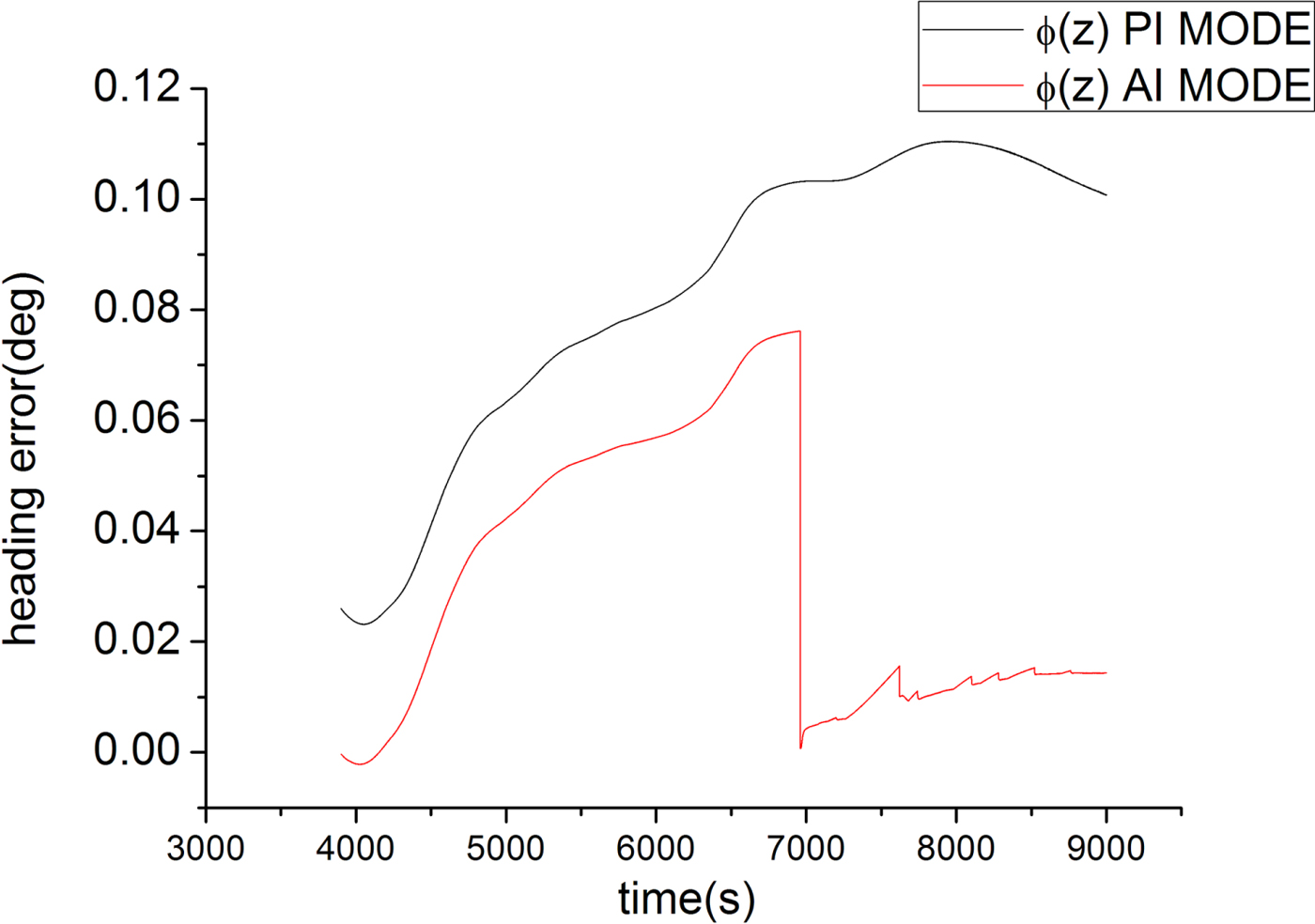
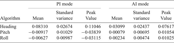
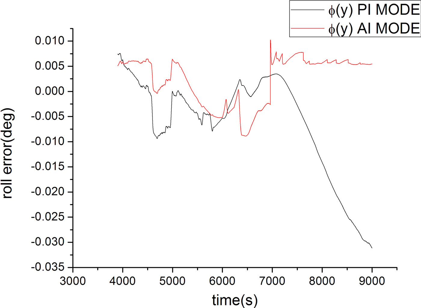
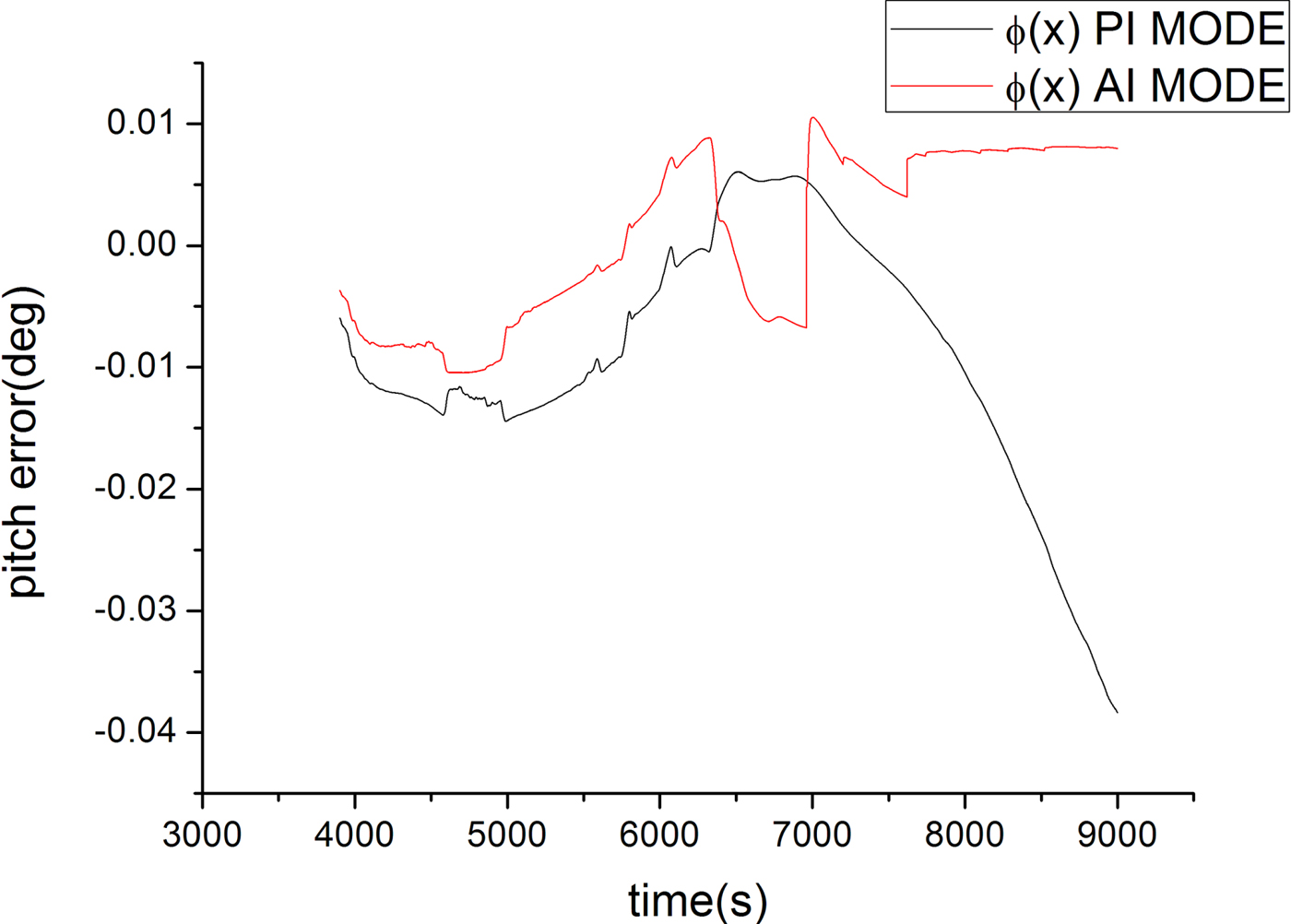
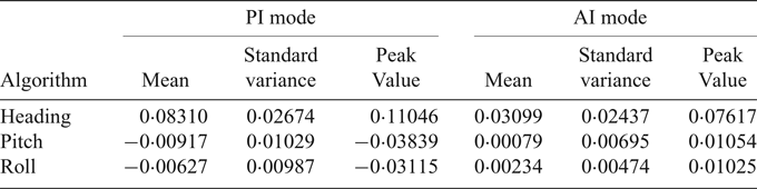
In the experiment, an accurate attitude reference was not available, thus we took the attitude of the integrated INS/GPS as the reference to compare the attitude error of the proposed method and pure inertial navigation. When the filter came to the steady state after 3,900 s, we compared the attitude error for the following 5,100 s. Figures 10–12 show the comparison results. PI MODE refers to pure inertial navigation and AI MODE is the proposed method. The attitude error peak values after the filter came to a steady state and mean and standard variance are listed in Table 2. The results show that the proposed method has higher attitude accuracy and can limit the attitude error.
Roll error.
Pitch error.
Heading error.

Attitude error in the experiment.
6. CONCLUSION
In this paper, a dynamically-aided inertial navigation method has been proposed to improve the ocean vehicle attitude accuracy. Additional observations were derived based on dynamic knowledge to update the filters. The proposed method includes two parts: the dynamic identification algorithm and the utilisation of dynamic constraints to derive additional observations. The simulation and experiment results show that the proposed dynamically-aided method has a relatively higher attitude accuracy than the pure inertial navigation method and can provide satisfactory navigation parameters over a long period. When external information, such as GPS and DVL, is in outage or unavailable, the proposed method can be a good backup. Without the need for external equipment, both the character of autonomy and integrity of Inertial Navigation System (INS) are enhanced. It is especially applicable to large warships with small mobility.