Debating the Merits of LDVs

For many decades, including LDVs in regression analysis was routine, but Keele and Kelly (Reference Keele and Kelly2006) note that “the current default response to lagged dependent variables is suspicion, if not outright rejection.” Beck and Katz (Reference Beck and Katz2011) observe that the Achen (Reference Achen2000) critique of LDVs remains very influential in political science but argue that “contra Achen, there is nothing pernicious in the use of a model with a lagged dependent variable.”Footnote ¹ The question about the appropriateness of including LDVs in regression analysis is ongoing in many literatures: some papers cite Achen (Reference Achen2000) to argue against their inclusion, while others cite Keele and Kelly (Reference Keele and Kelly2006) to argue for their inclusion.

For instance, studies in the congressional elections literature modeling the determinants of vote shares have traditionally included a LDV (Gelman and King Reference Gelman and King1990; Cox and Katz Reference Cox and Katz1996; Jacobson Reference Jacobson1996), while some more recent studies have preferred models that exclude the LDV (Canes-Wrone, Brady and Cogan Reference Canes-Wrone, Brady and Cogan2002; Carson et al. Reference Carson, Koger, Lebo and Young2010). A newer literature on economic voting has debated the direction of the relationship between individual political preferences and opinions about the state of the economy. A key point of contention in this literature has been whether the models used should contain LDVs (Evans and Pickup Reference Evans and Pickup2010) or not (Lewis-Beck Reference Lewis-Beck2006; Lewis-Beck, Nadeau and Elias Reference Lewis-Beck, Nadeau and Elias2008). Literature in the American and comparative contexts have debated factors influencing levels of government spending, with some studies using the LDV (Garrett and Mitchell Reference Garrett and Mitchell2001) and others criticizing its use (Achen Reference Achen2000; Huber and Stephens Reference Huber and Stephens2001; Plümper, Troeger and Manow Reference Plümper, Troeger and Manow2005). Findings about the effect sizes of variables such as the unemployment rate and ideological composition of governments vary based on whether the LDV is included (Garrett and Mitchell Reference Garrett and Mitchell2001) or excluded (Plümper, Troeger and Manow Reference Plümper, Troeger and Manow2005). Plümper, Troeger and Manow (Reference Plümper, Troeger and Manow2005) and Huber and Stephens (Reference Huber and Stephens2001) also criticize the use of LDVs in the broader comparative political economy literature, arguing that they unduly suppress the explanatory power of other variables.

The Achen (Reference Achen2000) critique of LDVs has been cited in literature using time series data and also in literature using panel data (Plümper, Troeger and Manow Reference Plümper, Troeger and Manow2005; Carson et al. Reference Carson, Koger, Lebo and Young2010). When using LDVs in panel models, a different issue than the one discussed by Achen (Reference Achen2000) can arise: in panel models that have a LDV and fixed effects, researchers need to be attentive to the problem of Nickell (Reference Nickell1981) bias in data with low T (with fixed T, Nickell bias does not go to 0, even as N→∞), a subject I discuss in Online Appendix H.

In general, regressions that exclude the LDV often obtain larger coefficient estimates for independent variables, compared with regressions that include the LDV. Consequently, the choice about whether or not to include a LDV in regression analysis would likely have a substantial impact on the conclusions of empirical analyses across a number of literatures. To illustrate the problems with including LDVs in regression analysis, Achen (Reference Achen2000) sets up the following data-generating process (where Y _t and X _t are stationary time series):

The independent variable Y _t is a function of Y _t−1, an independent variable X _t , and an autoregressive error term u _t . X _t and u _t are autoregressive functions with independent and identically distributed (IID) error terms e _1t and e _2t . Under Equations 1–3, Achen (Reference Achen2000) shows that a regression of Y _t on Y _t−1 and X _t will produce biased estimates of β (underestimating the actual coefficient), even though Y _t−1 is actually a part of the data-generating process. Achen (Reference Achen2000) uses this result to argue against the use of LDVs in regression analysis. Keele and Kelly (Reference Keele and Kelly2006) argue that when the LDV is part of the data-generating process, excluding it will induce omitted variable bias. Keele and Kelly (Reference Keele and Kelly2006) take the data-generating process specified by Achen (Reference Achen2000) and use Monte Carlo simulation to test which model specifications produce the best coefficient estimates (under a variety of parameter values for α and ϕ). They find that a regression of Y _t on X _t and Y _t−1 produces estimates with relatively low bias compared with other models (such as just regressing Y _t on X _t ), except under high levels of autocorrelation in the error term (high values of ϕ). But the problems in estimating the coefficient of the independent variable, β, arise because neither Achen (Reference Achen2000) nor Keele and Kelly (Reference Keele and Kelly2006) specify the correct regression model, given the data-generating process.

Most of the debate has centered on whether we get better coefficient estimates by regressing Y _t on: (1) X _t or (2) X _t and Y _t−1. But given the data-generating process in Equations 1–3, both of these regressions are mis-specified and suffer from omitted variable bias. This becomes apparent when we use simple substitution to re-write Equation 1 as

We arrive at Equation 4 as follows. We can put Equation 1 in terms of u _t , giving us u _t =Y _t −αY _t−1−βX _t . At time t−1, this expression will be u _t−1=Y _t−1−αY _t−2−βX _t−1. Substituting this into Equation 3 gives us

This expression for u _t can be substituted back into Equation 1, giving us

Equation 4 has an IID error term and also includes regressors X _t−1 and Y _t−2. The reason that a regression of Y _t on Y _t−1 and X _t produces biased estimates of β is that the regression improperly excludes X _t−1 and Y _t−2, violating the exogeneity assumption required for ordinary least squares (OLS). If X _t−1 and Y _t−2 are excluded, independent variables X _t and Y _t−1 will be correlated with the error term, u _t , resulting in omitted variable bias (u _t is a function of Y _t−1, Y _t−2, X _t−1, and e _2t ).Footnote ² In Equation 4, the error term is not correlated with any of the independent variables, satisfying the exogeneity assumption.Footnote ³ Equation 4 is a special case of the autoregressive distributed lag (ADL) (2,1) model (Beck and Katz Reference Beck and Katz2011).Footnote ⁴ Neither Achen (Reference Achen2000) nor Keele and Kelly (Reference Keele and Kelly2006) consider the properties of estimates of β derived from a regression based on Equation 4.

Some researchers specify their dependent variable as Y _t −Y _t−1 to avoid using a LDV in their regression model. Morgan and Winship (Reference Morgan and Winship2007) discuss situations where one may prefer a LDV model (control for Y _t−1 and treatment D) or a model where Y _t −Y _t−1 is used as the dependent variable (control for treatment D). Morgan and Winship (Reference Morgan and Winship2007) note that in some cases the latter model will identify a treatment effect, but the former model will not. But the latter model (with Y _t −Y _t−1 as the dependent variable) amounts to introducing a restriction that the coefficient of Y _t−1 (which in Equation 4 is α+ϕ) is equal to 1. No such restriction is present in the data-generating process in Equations 1–3 and as recommended by Hendry (Reference Hendry1995) and De Boef and Keele (Reference De Boef and Keele2008), any restrictions on coefficients in a general model should be tested.Footnote ⁵ Next, I use Monte Carlo simulation to show that a regression based on Equation 4 produces much better coefficient estimates for the effect of β than either regressing Y _t on X _t or regressing Y _t on X _t and Y _t−1. This finding holds across weakly to strongly dynamic processes (where 0<α<1) and across weakly to strongly autocorrelated error terms (where 0<ϕ<1).

As is standard when using time series models, X _t and Y _t need to be stationary. The stationarity conditions for X _t , which is an AR(1) process, are straightforward: if |ρ|<1, then X _t will be a stationary time series. However, the stationarity conditions for Y _t are slightly more complicated because it is a second-order autoregressive time series. The following three conditions are necessary for Y _t to be stationary:

All of the Monte Carlo examples considered in this paper satisfy the stationarity conditions, but before proceeding with any time series modeling, it is important for researchers to test if the time series data in question is in fact stationary. Online Appendix D includes a derivation of the stationarity conditions for the general ADL(2,1) model and from there the stationarity conditions for the Equation 4 time series follow through simple substitution. The stationarity conditions for an autoregressive model of order p, i.e., α _p (L)y _t =ε _t , can be determined by calculating the conditions under which the roots of α _p (L) lie outside the unit circle (Wei Reference Wei2005).Footnote ⁶ Researchers can use this method to determine the formal conditions required for stationarity for higher order autoregressive models.

Keele and Kelly (Reference Keele and Kelly2006) claim that the data-generating process in Equations 1–3 requires that |α+ϕ|<1 for stationarity, but add the caveat that it is only “roughly true” in a footnote, referring readers to an online appendix for full stationarity conditions for this process. But this condition is not even roughly true: consider the case where α=0.9 and ϕ=0.9. Under the stationarity conditions derived above, the data-generating process in Equations 1–3 would still be stationary, even at these high values of α and ϕ. In their online appendix, Keele and Kelly (Reference Keele and Kelly2006) recognize that the data-generating process in Equations 1–3 is second-order autoregressive for Y _t and claim that the stationarity conditions for such a process require that |α+ϕ−αϕ|<1. But this is also not the correct stationarity condition, as it would imply that α+ϕ−αϕ−ϕ>−1 when the sign is reversed on the absolute value, which we can see conflicts with the third stationarity condition listed above. It is important to derive the stationarity conditions when considering the properties of higher order autoregressive models because their stationarity conditions will be much more complex than the stationarity conditions for a first-order autoregressive model.

Monte Carlo Simulations

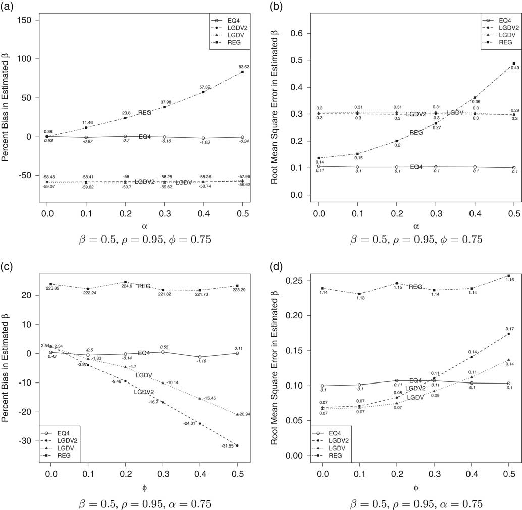
I replicated the Monte Carlo simulations performed by Keele and Kelly (Reference Keele and Kelly2006) and found that the percent bias in estimates of β from Equation 4 was consistently much lower than the percent bias in any of the estimators considered by Keele and Kelly (Reference Keele and Kelly2006).Footnote ⁷ Figures 1(a) and 1(c) show the percent bias in estimates of β under four different models: (1) EQ4, a regression model estimated with an ADL(2,1) model, of which Equation 4 is a special case (see Online Appendix A for estimation details); (2) LGDV2, a regression of Y _t on Y _t−1, Y _t−2, and X _t ; (3) LGDV, a regression of Y _t on Y _t−1 and X _t ; and (4) REG, a regression of Y _t on X _t (Keele and Kelly Reference Keele and Kelly2006 included the LGDV2, LGDV, and REG regressions in their analysis). I did not replicate the Prais–Winsten, Cochrane–Orcutt, or autoregressive moving average models used by Keele and Kelly (Reference Keele and Kelly2006), however, the EQ4 estimation of β had a much lower level of bias than the estimates of those models.Footnote ⁸ The Monte Carlo simulations were performed using 1000 trials and data sets with 100 observations (T=100).

Fig. 1

(a) Percent bias in estimates of β conditional upon varying levels of α (dynamic parameter) (b) Root mean square error of estimates of β conditional upon varying levels of α (dynamic parameter) (c) Percent bias in estimates of β conditional upon varying levels of ϕ (autoregressive error parameter) (d) Root mean square error of estimates of β conditional upon varying levels of ϕ (autoregressive error parameter)

Before turning to the Monte Carlo results, a note of caution is in order. In small T time series data, OLS regressions that include a LDV will produce biased coefficient estimates for the LDV, even if the data-generating process is modeled correctly (Hurwicz Reference Hurwicz1950). The type of bias identified by Hurwicz (Reference Hurwicz1950) quickly approaches 0 as T grows larger. Thus, the estimates of β in Equation 4 will be asymptotically unbiased, but will suffer from bias for finite T.

In Figure 1(a), we fix β=0.5, ρ=0.95, and ϕ=0.75, and allow α to vary between 0 and 0.5. Figure 1(a) shows that EQ4 has the lowest percentage bias out of all other estimators when α>0 and the bias never exceeds ±2 percent. The only level of α where Equation 4 does not provide the lowest percentage bias is where α=0, but in this case, the data-generating process is not dynamic so it is unnecessary to include lags of Y in the regression. But even with weakly dynamic effects (low levels of α), EQ4 provides the lowest percent bias in β out of all estimators. Figure 1(b) shows that under the parameter values used in Figure 1(a), EQ4 has the lowest root mean square error (RMSE) out of all of the specifications considered.

In Figure 1(c), we fix β=0.5, ρ=0.95, and α=0.75, and allow ϕ to vary between 0 and 0.5 (note for the purposes of displaying the data properly, the REG biases had to be shifted downward on the y-axis in Figures 3 and 4). Across all values of ϕ, EQ4 provides estimates of β with lower percent bias (under 1.2 percent) than the other regression models specified. Figure 1(d) shows the RMSE of the estimators of β under the parameter values used in Figure 1(c). EQ4 has a slightly higher RMSE than LGDV2 and LGDV at lower levels of error autocorrelation (ϕ≤0.2), but lower RMSE at higher levels of autocorrelation. The RMSE and the percent bias in the REG specification are considerably higher, suggesting that under the data-generating process in Equations 1–3, excluding lagged variables will produce very poor estimates of β.

The Monte Carlo simulations show that under the theoretical data-generating process specified by Achen (Reference Achen2000), a regression of Y _t on Y _t−1, Y _t−2, X _t and X _t−1 (the EQ4 specification) produces very accurate estimates of the effect of X _t on Y _t and greatly outperforms all other specifications considered. Furthermore, the Monte Carlo simulations show that excluding lagged variables from regression analysis will cause us to overestimate the effect of X _t on Y _t . The REG model overestimates values of β and this bias grows worse as the data-generating process gets more strongly dynamic (higher values of α). But failing to specify the correct lag structure will also induce bias. The LGDV model underestimates values of β and this bias becomes worse as the level of autocorrelation in the error term (ϕ) increases, consistent with the results shown by Achen (Reference Achen2000). Neither the REG nor the LGDV models are appropriate given the data-generating process in Equations 1–3.

Of course, researchers are rarely in the position where they actually get to observe the data-generating process they wish to study, so the choice of an appropriate model might not be straightforward. For instance, suppose a researcher was studying a data-generating process that (unknown to the researcher) was generated by Equations 1–3. How should the researcher proceed and would the researcher be able to determine that a model based on Equation 4 was the proper model for their data? De Boef and Keele (Reference De Boef and Keele2008) argue that to model time series processes, researchers should start with a general model, like the ADL(1,1) model and then test additional restrictions.Footnote ⁹ De Boef and Keele (Reference De Boef and Keele2008) note that researchers often start their analysis with restricted versions of general models, without testing whether the restrictions are appropriate, which can cause biased coefficient estimates. Hendry (Reference Hendry1995) explains that the ADL(1,1) model is a very general model, so it is uncommon to detect a misspecification. However, if residual autocorrelation is detected in the ADL(1,1) model, Hendry (Reference Hendry1995) recommends using an even more general model, such as one with more lags of the dependent variable. Wooldridge (Reference Wooldridge2012) also discusses how adding lags of the dependent variable to a regression model can purge error autocorrelation. Following this strategy would lead us to the following modeling approach: begin with an ADL(1,1) model, test for residual autocorrelation, and add lags of the dependent variable until the autocorrelation has been purged from the residuals.

Suppose we took this approach to modeling the Monte Carlo data considered previously. Table 9 and Figure 5 in Online Appendix A show the percentage of Monte Carlo simulations where the EQ4 and ADL(1,1) models detect autocorrelation (using a Ljung–Box test and rejecting the null of no autocorrelation for p-values below 0.05).Footnote ¹⁰ Starting with the ADL(1,1) model, we detect autocorrelation more frequently as ϕ and α increase (see Table 9 and Figure 5 in Online Appendix A). The EQ4 model has a white noise error term, so as expected, only a very small percentage of simulations would (incorrectly) detect autocorrelation in the residuals. Under a data-generating process that is strongly dynamic and has high error autocorrelation, we would be quite likely to detect autocorrelation, add Y _t−2 to the model, and then fail to reject the null of no autocorrelation (thus arriving at the correct model). However, under lower values of ϕ and α, the ADL(1,1) model often failed to detect residual autocorrelation. In these cases, a researcher using this modeling approach would stick with the ADL(1,1) model instead using the correct ADL(2,1) model (Equation 4 is a special case of this model). This would not be too problematic, as the ADL(1,1) model provides estimates of β that are quite close to the actual value. Table 1 shows that across all levels of α and ϕ, the estimates of β from the ADL(1,1) model have a percent bias of under 1 percent and a RMSE of comparable size to the EQ4 model. The Monte Carlo simulations confirm that the modeling approach advocated by Hendry (Reference Hendry1995) and De Boef and Keele (Reference De Boef and Keele2008) of starting with a general model and “testing down” would produce a very accurate estimate of β while a blanket restriction against using LDVs would lead to biased estimates of β.

Table 1

Percent Bias and Root Mean Square Error (RMSE) in Autoregressive Distributed Lag (ADL) (1,1) Model (Under Varying Levels of α and ϕ)

Note: β=0.5, ρ=0.95.

ϕ=0.75 under varying levels of α.

α=0.75 under varying levels of ϕ.

Although the ADL(1,1) and EQ4 models return close estimates for β, the immediate effect of X _t on Y _t , the two models perform quite differently in terms of estimating the long-run effect of X _t on Y, as will be shown later. In certain cases (particularly under lower values of ρ), the ADL(1,1) model suffers from quite severe bias compared with the EQ4 model, when it comes to estimating the long-run effects. This would substantially raise the stakes for which model a researcher ends up choosing, particularly if there is a close call as to whether there is autocorrelation in the residuals after fitting the ADL(1,1). In the example above, we used the conventional 0.05 level of significance for rejecting the null hypothesis of no autocorrelation. But if the p-value for the Ljung–Box test is slightly above 0.05, there is a strong possibility that there actually is autocorrelation in the residuals and that by not including Y _t−2 in the model, the reported long-run effects might be very biased. In cases where it is a close call as to whether there is remaining residual autocorrelation, it would be prudent for researchers to report the estimated long-run effects of both the ADL(1,1) and the ADL(2,1) model so that their results could be compared and readers would be more aware of how the estimates regarding long-run effects differed based on the choice of model.

Asymptotic Properties of the Models

While it is usually preferable to directly calculate the biases of various models rather than relying upon Monte Carlo, the Monte Carlo simulations discussed previously are necessary in order to consider how each of the models performs with finite T. Autoregressive models with finite T suffer from Hurwicz bias, but there is no general formula that would allow the calculation of this bias which is why it is difficult to use autoregressive models when T is very small. Hurwicz bias has only been formally calculated for a very limited set of models due to computational difficulty (Keele and Kelly Reference Keele and Kelly2006). However, if we examine the models under the condition that T→∞, we can calculate formulas for the biases of the models considered earlier. The bias considered here is the bias in the effect of X _t on Y _t (i.e., $$\hat{\beta }$$ ).

Because we know the full set of independent variables present in the data-generating process discussed in this paper, we can perform a calculation of the omitted variable bias for the REG, LGDV, and LGDV2 models. Suppose matrix X represents the variables included in the model of interest, while variable Z represents the variables that are actually in the data-generating process, but are omitted from the model of interest. Let vector y represent variable Y _t and vector ε represent e _2t . The data-generating process under this specification is y=Xβ+Zγ+ε. The expected value of the estimated coefficients of the model of interest are: β+(X′X)⁻¹ X′Zγ, where β denotes the true coefficient values and (X′X)⁻¹ X′Zγ represents the omitted variable bias. For notational simplicity for the bias formulas, let us use the following: a=X′ _t X _t , b=X′ _t−1 X _t , c=X′ _t Y _t , d=Y′ _t−1 Y _t , and f=Y′ _t Y _t . With these definitions, we are still not in a position to make exact calculations of the bias, but in Online Appendix G, I provide derivations of a, b, c, d, and f in terms of the model parameters for the ADL(2,1) model (from there simple substitution will derive the formulas in terms of the parameters of the EQ4 model). Now let us turn to a discussion of the bias present in the REG, LGDV2, and LGDV models.

The REG model includes X _t , but leaves out X _t−1, Y _t−1, and Y _t−2. The bias for this model isFootnote ¹¹

Notice that each term in the bias calculation contains ρ, the autoregressive coefficient in the data-generating process for X _t . What this means is that the source of the bias in the REG model comes from leaving out X _t−1. If X _t were not an autoregressive time series (meaning ρ=0), then the REG model would provide an asymptotically unbiased estimate of the effect of X _t on Y _t . But as the autoregressive parameter of X _t increases, the bias of the REG model grows worse. Using this bias formula, we can find a straightforward calculation of the bias of the REG model under various values of α, ϕ, and ρ. Figure 2(a) shows a contour plot of the percent bias in β of the REG model where ρ=0.95, and α and ϕ both range from 0 to 0.9. The bias is largely independent of shifts in the value of ϕ, but grows worse as α increases. Even at relatively low values of α, such as 0.2, the bias of the REG model is over 20 percent. But suppose we were dealing with a data-generating process where ρ was much smaller. Figure 2(b) shows a contour plot of the percent bias in β for the REG model under varying values of α and ρ, where ϕ=0.75. As we saw in Figure 2(a), the bias is largely independent of the value of ϕ, so we can pick an arbitrary value of ϕ and observe how the bias changes as a function of α and ρ. The bias of the REG model will be small if both α and ρ are small, but if either parameter starts getting large, that can mean there is substantial bias, even if the other parameter is small. Once α and ρ both go over about 0.3, the bias will be in excess of 10 percent. That means that if X _t and Y _t are even weakly autoregressive processes, the REG model will produce noticeably biased estimates of β. Given these drawbacks, it is much better if we follow the approach of starting with a more general model and not prematurely assuming that the coefficient of X _t−1 is 0, as we do if we use the REG model.

Fig. 2

(a) Percent bias in REG model, β=0.5, ρ=0.95 (b) Percent bias in REG model, β=0.5, ϕ=0.75 (c) Percent bias in LGDV2 model, β=0.5, ρ=0.95 (d) Percent bias in LGDV2 model, β=0.5, α=0.75

Now let us consider the bias of the LGDV2 model, which is

In cases where ϕ=0 (no autocorrelation in the error term of Y _t ) or ρ=0 (X _t is not a dynamic process), the LGDV2 model will provide an asymptotically unbiased estimate of β. But we can see that as ϕ increases and as ρ increases, the bias steadily grows worse. Figure 2(c) shows the bias in the estimates of β under the LGDV2 model where ρ=0.95 and α and ϕ range from 0 to 0.9. As the error autocorrelation increases (higher values of ϕ), the bias in the LGDV2 model gets more negative. Even at a modest level of ϕ, such as 0.2, the bias is around −15 percent, and once ϕ gets to 0.8, the bias is up around −70 percent. Figure 2(d) shows the bias in the estimate of β under varying values of ϕ and ρ when α=0.75. As we saw in Figure 2(c), the bias in the LGDV2 model is largely independent of values of α, allowing us to pick an arbitrary value for α and check how the bias varies as a function of ϕ and ρ. The bias will be low if ϕ and ρ are both small, but if either parameter gets large, the bias can get large even if the other parameter is small. If ϕ and ρ are both >0.4, the bias in the model will exceed −10 percent and if both parameters are >0.6, the bias will exceed −30 percent.

Finally, let us consider the bias in the estimate of β under the LGDV model. The bias of the LGDV model is

All of the terms in the numerators contain ϕ and ρ, meaning that if either ϕ=0 or ρ=0, the asymptotic bias of the LGDV model will be 0. Figure 3 shows the percent bias in the LGDV model where ρ=0.95 and α and ϕ range from 0 to 0.9. Given a certain value of ϕ, as α increases, the bias will stay constant at first, as with the LGDV2 model, but after a certain point, the bias starts dropping as α increases. For instance, if ϕ=0.75, the bias is about −65 percent when α=0.3, but it falls to about −50 percent when α=0.75. Figure 4 shows the bias in estimates of β under varying values of ϕ and ρ, where α is 0, 0.2, 0.4, and 0.6. We can see that as α increases, the level of bias for any given level of ϕ and ρ gets less severe. As ϕ and ρ increase, the LGDV model gets more negatively biased.

Fig. 3

Percent bias in LGDV model, β=0.5, ρ=0.95

Fig. 4

Percent bias in LGDV model, β=0.5. Starting at the top left graph and running clockwise, values of α are as follows: α=0, α=0.2, α=0.6, α=0.4.

Under the REG model, we are only able to obtain asymptotically unbiased estimates of β if it is the case that X _t is not a dynamic process (ρ=0). With the LGDV and LGDV2 models, we can only obtain asymptotically unbiased estimates if X _t is not a dynamic process (ρ=0) or there is no error autocorrelation in Y _t (ϕ=0). Rather than hope that these conditions are met when picking a model, we can use a general model like the ADL(1,1) and then test if these restrictions hold or not.

In the last section, the Monte Carlo results demonstrated that the ADL(1,1) model was able to provide very accurate estimates of β even though that model improperly excludes Y _t−2. The bias calculation shows that the bias of the ADL(1,1) model approaches zero when T→∞ (see Online Appendix E). As long as we include X _t−1 in our regression, we will be able to get an unbiased estimate of β. But where this could be more problematic is when we are interested in estimating the long-run effect of X _t on Y _t . In a dynamic model, the effect of a shift in X at time t on Y is not just limited to time t, the effect is felt in time t+1, t+2, and onward (though the effect necessarily goes to 0 as T→∞ as a condition for stationarity). Next, we turn to a discussion about estimating the long-run effect of a shift in X _t on Y.

Long-Run Effect of X on Y

Up to now, we have considered the biases present in estimates of β, which is the one-period effect of X _t on Y _t . But in a dynamic data-generating process, the effect of X _t on Y will continue to be felt in additional periods, so researchers will often be interested in estimating the total effect of a change in X _t on Y. Because of the stationarity property, the effect of X _t on Y must diminish toward 0 as T→∞, meaning that we can calculate the total size of the effect over time. In an ADL(2,1) model, the long-run effect of X _t on Y will beFootnote ¹²

Note that under the data-generating process in Equations 1–3, we can substitute in for the values of α ₁, α ₂, β ₁, and β ₂. Based on the data-generating process laid out in Equations 1–3, the long-run effect of X _t on Y will be

Because X _t is a dynamic time series along with Y _t , we must account for that in the long-run estimation of the effect of X _t on Y, by estimating ρ, the autoregressive parameter of X _t (see Online Appendix F for details on the derivation of the long-run effect formula). Most discussions about estimating the long-run effect of some variable X _t on a dynamic process Y _t assume that X _t is not dynamic and give a formula such as β/(1−α) for estimating the long-run effect. But given that X _t is indeed a dynamic process, as per Equation 2, neglecting to also include 1−ρ in the denominator will mean our estimate of the long-run effect of X _t on Y will be too small.

Keele and Kelly (Reference Keele and Kelly2006) consider the same data-generating process discussed in this paper, but estimate the long-run effect of X _t on Y as β/(1−α). Their primary model estimates for β and α are coming from regressing Y _t on Y _t−1 and X _t , which as discussed earlier will produce biased estimates of β. But what is particularly problematic for estimating long-run effects is that their formula does not include (1−ρ) in the denominator. The long-run effect formula used by Keele and Kelly (Reference Keele and Kelly2006) is for a process where a shock in X at time t does not affect future values of X _t . In that scenario, the shock in X at time t affects Y through the variable X _t only at time t, but in future periods, the effect persists solely through the lags of Y. Formally, Keele and Kelly (Reference Keele and Kelly2006) are asserting that the shock in X has an effect on Y of β at time t (via X _t ), then continues to be felt via Y _t−1 in subsequents periods, i.e., βα at t+1, βα ² at t+2, and so on. The sum of these effects is a geometric series $$\beta {\times}\mathop{\sum}\nplimits_{i{\,\equals\,}0}^\infty \alpha ^{i} $$ , which converges to β/(1−α) so long as |α|<1. However, the data-generating process considered in this paper, as well as Keele and Kelly (Reference Keele and Kelly2006) and Achen (Reference Achen2000) specifies that X _t follows an AR(1) process, meaning that a shock in X at time t will affect future values of X _t . Thus, a shock in X at time t would affect Y in future periods both through X _t and lags of Y. As shown in Online Appendix F, the correct formula for the long-run effect of X _t on Y under Equations 1–3 includes 1−ρ in the denominator.

De Boef and Keele (Reference De Boef and Keele2008) examine the properties of models that are special cases of the ADL(1,1) model, as well as ECM. De Boef and Keele (Reference De Boef and Keele2008) give the formula for the long-run effect of X _t on Y in the ADL(1,1) as (β ₁+β ₂)/(1−α ₁).Footnote ¹³ In this case, they must assume that a shock in X at time t does not affect future values of X. If that assumption holds, a shock in X at time t will affect Y at time t through X _t , will affect Y at time t+1 through X _t−1 and Y _t−1 and in all future periods will only affect Y through Y _t−1. Unlike Keele and Kelly (Reference Keele and Kelly2006) or this paper, De Boef and Keele (Reference De Boef and Keele2008) does not conceptualize X _t as an autoregressive process, so it could be argued that this formula is still correct when X _t is not itself dynamic.

One of the core arguments in De Boef and Keele (Reference De Boef and Keele2008) and Hendry (Reference Hendry1995) is that researchers should start with general models and not assume any restrictions without testing them. Assuming that X _t is not a dynamic process amounts to introducing a restriction on the data-generating process of X _t . The long-run effect calculation in De Boef and Keele (Reference De Boef and Keele2008) relies on such an assumption, but De Boef and Keele (Reference De Boef and Keele2008) do not inform researchers to examine the time series structure of X _t before proceeding with a calculation of long-run effects, which is tantamount to introducing an untested restriction on the data-generating process. However, there is one particular example in De Boef and Keele (Reference De Boef and Keele2008) that does specify the time series structure of X _t : in Equation 15 in their paper, they consider the case of an ADL(1,1) model where X _t is an AR(1) time series and again offer the formula (β ₁+β ₂)/(1−α ₁) as the long-run effect of a shock in X at time t on Y. In that context, the formula offered by De Boef and Keele (Reference De Boef and Keele2008) is not correct, because shocks in X at time t will affect future values of Y through X _t , X _t−1, and Y _t−1. The correct long-run effect of X _t on Y would be (β ₁+β ₂)/[(1−ρ)(1−α ₁)], where ρ is the coefficient of X _t−1 in the data-generating process for X _t .

In order to maintain consistency with the approach of starting with a general model and testing any restrictions, researchers should examine the time series structure of X _t prior to proceeding with a calculation of the long-run effect of X _t on Y. If X _t follows a different time series structure than the AR(1), the long-run effects for an ADL(2,1) model could be different than the formula shown earlier in this section. Online Appendix F provides a derivation for the long-run effect of X _t on Y using the data-generating process in Equations 1–3.

We can estimate ρ using a regression of X _t on X _t−1 and the other parameters can be estimated using Equation 4. The presence of Hurwicz bias with finite T means that when ρ is large, even small biases in the estimate of ρ could substantially bias the estimates of long-run effects. For instance, suppose β=0.5, α=0.75, and ρ=0.95 and we estimate both α and β without bias, but due to Hurwicz bias, our expected value for the estimate of ρ is 0.93. The bias in the estimate of ρ is a seemingly inconsequential −2.1 percent, but the bias in the estimated long-run effect of X _t on Y is substantial: about −28.6 percent.

But consider if ρ=0.75 and our estimate of ρ has an expected value of 0.73. The bias in the estimate of ρ is now about −2.7 percent, not much different from when ρ=0.95. But in this scenario, the bias in the long-run effect of X _t on Y drops to −7.4 percent. What this demonstrates is that when we estimate the long-run effects of variables in autoregressive processes, even a small amount of Hurwicz bias can introduce a sizeable bias if the autoregressive parameter is high. Because there is not a general formula that allows for the correction of Hurwicz bias, in practice it will be hard to say just how severe the bias is when we are not in a position to look behind the scenes in a data-generating process. With this in mind, let us turn to an examination of Monte Carlo simulations regarding the accuracy of estimates of the long-run effects using each of the models considered earlier.

For the LGDV2 model, we do not have a coefficient for X _t−1, so we will estimate the long-run effect without β ₂, so the formula for calculating the long-run effect of X _t on Y will be β ₁/[(1−ρ)(1−α ₁−α ₂)]. For the LGDV model, we do not have a coefficient for either X _t−1 or Y _t−2, so the formula will be β ₁/[(1−ρ)(1−α ₁)]. The REG model is not autoregressive, meaning we do not have coefficients for X _t−1, Y _t−1, or Y _t−2, so the formula will be β ₁/(1−ρ).

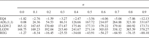
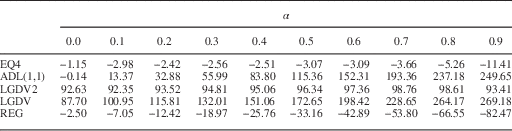
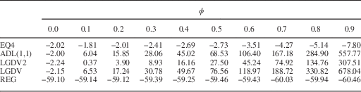
Tables 2–4 show the percent bias in these models, along with the EQ4 model, where α ranges from 0 to 0.9, ϕ=0.75. Parameter ρ is 0.25 in Table 2, 0.55 in Table 3, and 0.95 in Table 4. The number of Monte Carlo simulations is set at 30,000 and I use the median percent bias rather than the mean percent bias, because the presence of outliers (particularly when ρ is large) can distort the results and makes it harder to see the patterns with varying levels of α. Nevertheless, I also include tables showing the mean percent bias in Online Appendix B. When ρ is 0.25 or 0.55, the bias in the EQ4 model ranges from around −2 percent when α=0 to about −12 percent when α=0.9. The bias in the EQ4 model is around −15 percent when ρ=0.95. The percent bias in the ADL(1,1) model grows very rapidly as α increases and becomes quite severe by the time α=0.9 (when ρ is 0.25 or 0.55). But when ρ=0.95, the ADL(1,1) model underestimates the long-run effect when α<0.45 and overestimates the effect when α>0.45. The LGDV and LGDV2 models have severe bias even when α=0 and it grows worse as α increases (when ρ is 0.25 or 0.55). When ρ=0.95, the LGDV model has negative bias when α<0.2 and positive bias when α>0.2. When ρ=0.95, the LGDV2 model has a bias ranging from around −6 percent when α=0 to about −11 percent when α=0.9. The REG model becomes more negatively biased as α increases and as we would expect, it performs about as well as the EQ4 model when α=0 (meaning that Y _t is not dynamic).

Table 2

Percent Bias in Long-Run Estimates of X _t on Y Conditional Upon Varying Levels of α (Dynamic Parameter); ρ=0.25

Note: β=0.5, ρ=0.25, ϕ=0.75.

ADL=autoregressive distributed lag.

Table 3

Percent Bias in Long-Run Estimates of X _t on Y Conditional Upon Varying Levels of α (Dynamic Parameter); ρ=0.55

Note: β=0.5, ρ=0.55, ϕ=0.75.

ADL=autoregressive distributed lag.

Table 4

Percent Bias in Long-Run Estimates of X _t on Y Conditional Upon Varying Levels of α (Dynamic Parameter); ρ=0.95

Note: β=0.5, ρ=0.95, ϕ=0.75.

ADL=autoregressive distributed lag.

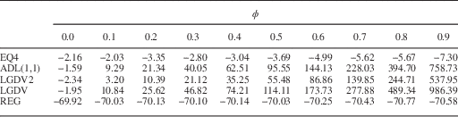
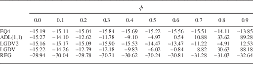
Tables 5–7 show the percent bias in these models where ϕ ranges from 0 to 0.9, α=0.75. Parameter ρ is 0.25 in Table 5, 0.55 in Table 6, and 0.95 in Table 7. When ρ is 0.25 or 0.55, the bias in the EQ4 model ranges from about −2 percent when ϕ=0 to about −8 percent when ϕ=0.9. When ρ=0.95, the bias is around −15 percent. The ADL(1,1) model goes from slightly underestimating the effect of X _t on Y when ϕ is small to massively overestimating it when ϕ is much larger (when ρ is 0.25 or 0.55). The bias grows quite quickly, so the ADL(1,1) model will overestimate the long-run effect even at low levels of ϕ. When ρ=0.95, the ADL(1,1) model behaves differently, going from underestimating the long-run effect when ϕ<0.6 and overestimating the effect when ϕ>0.6. The bias in the LGDV and LGDV2 models gets larger as α increases, when ρ is 0.25 or 0.55. However, when ρ is 0.95, the bias of the LGDV model only gets substantial when ρ≥0.7, while the LGDV2 model performs comparably to the EQ4 model. The bias of the REG model does not vary much with ϕ, but the bias tends to drop as ρ increases, going from about −70 percent when ρ=0.25 to about −31 percent when ρ=0.95.

Table 5

Percent Bias in Long-Run Estimates of X _t on Y Conditional Upon Varying Levels of ϕ (Autoregressive Error Parameter); ρ=0.25

Note: β=0.5, ρ=0.25, α=0.75.

ADL=autoregressive distributed lag.

Table 6

Percent Bias in Long-Run Estimates of X _t on Y Conditional Upon Varying Levels of ϕ (Autoregressive Error Parameter); ρ=0.55

Note: β=0.5, ρ=0.55, α=0.75.

ADL=autoregressive distributed lag.

Table 7

Percent Bias in Long-Run Estimates of X _t on Y Conditional Upon Varying Levels of ϕ (Autoregressive Error Parameter); ρ=0.95

Note: β=0.5, ρ=0.95, α=0.75.

ADL=autoregressive distributed lag.

EQ4 remains the best-performing model, though the LGDV2 comes close if ρ is large. In cases where ρ is not large, the LGDV and LGDV2 models perform very poorly. We can see that even in the case where T=100, Hurwicz bias can cause a substantial underestimation of the long-run effect of X _t on Y even with the best-performing model under higher levels of ρ. Additionally, although the ADL(1,1) model is able to estimate the coefficient of X _t just as well as the EQ4 model, it is much worse at estimating the long-run effect under most conditions. This bias is worse as ϕ increases, but as ϕ increases, we are also much more likely to detect autocorrelation in the errors with the ADL(1,1) and then add in Y _t−2. But as we saw earlier in the paper, at moderate levels of α or ϕ, there is a rather high rate of Type II errors, meaning that there is a possibility we could end up incorrectly failing to reject the null of no autocorrelation and then end up with a severely biased long-run estimate of the effect of X _t on Y. In cases where it is a potentially close call as to whether there is remaining residual autocorrelation in a model, researchers should report the results of both the ADL(1,1) and the ADL(2,1) estimates of the long-run effect of X _t on Y, so that readers are aware of how much a slight change in the regression specification could affect the estimates of the long-run effect.

In this set-up, we assume that the researcher is aware that X _t is a dynamic time series and estimates ρ as part of an effort to estimate the long-run effect of X _t on Y. Even though the LGDV, LGDV2, and REG models do not include the variable X _t−1, we assumed that a person utilizing these models to estimate the long-run effect of X _t would go ahead and estimate the autoregressive parameter of X _t , but not bother to try including X _t−1 in the time series. But given the discussion about the dangers of improperly restricted models, it would be a very bad idea if we already knew that X _t was an autoregressive time series and then went ahead and assumed that the coefficient of X _t−1 in the data-generating process for Y is 0. It is far better to start with a general model and test restrictions than it is to start with a restricted model and just hope that the restrictions do indeed hold.