


1 Introduction
In an aquifer or an oil reservoir, fluid is withdrawn by pumping from a recovery well. When the fluid is withdrawn from layers with different density, the withdrawn fluid will come from the layer surrounding the point of removal until the critical flow rate is reached [Reference Bear2,Reference Blake and Kucera3,Reference Giger6,Reference Hinch, Niordson and Olhoff7,Reference Muskat and Wyckoff15]. At this rate, the interface is drawn into a cusp shape, a process known as coning. Above the critical rate, the fluid from the adjacent layer will break through into the well. An example of where penetration is undesirable is water entering an oil recovery well or, in coastal regions, saline water entering a freshwater well.
Similar works exist in the practical agricultural and civil engineering literature, such as [Reference Childs4,Reference Kacimov and Obnosov9,Reference Van Deemter17,Reference Youngs18]. Youngs [Reference Youngs18] and Van Deemter [Reference Van Deemter17] provide some elegant mathematical solutions. A much more detailed bibliography of the relevant works can be found in the work of Kacimov and Obnosov [Reference Kacimov and Obnosov9].
Our concern in this work is the surface coning due to a line sink, and this was studied previously by [Reference Zhang, Hocking and Barry20], who found steady single-layer solutions that are limited at a pumping rate at which the water–oil interface forms an upward vertical cusp. Their solution did not rely on numerical methods but instead involved a fully analytical approach based on a hodograph transformation, a technique also employed with great utility by Youngs [Reference Youngs18]. The implementation of the flow as a line sink, or singular point, is clearly an approximation to a flow into a finite sized pipe or outlet, but finite pipes can be considered by enclosing the sink in small uniform regions with almost no effect on the results, and in large domains the sink will appear as a very small point in the flow region.
Similar studies were undertaken by Lukas et al. [Reference Lucas, Blake and Kucera11], Muskat and Wychoff [Reference Muskat and Wyckoff15], McCarthy [Reference McCarthy12] and Zhang et al. [Reference Zhang, Hocking and Barry20] with qualitatively similar results in all steady cases. More recently, Al-Ali et al. [Reference Al-Ali, Hocking and Farrow1] considered the flow into a line sink in a horizontally confined duct that was unbounded below and found both steady and unsteady solutions. Axisymmetric withdrawal solutions for the water coning problem with withdrawal from the upper layer of a stably stratified, two-layer fluid were computed by Lukas et al. [Reference Lucas, Blake and Kucera11], using an integral equation approach. They obtained steady-state solutions, valid up to pumping strengths at which the interface forms an upward vertical cusp. For pumping rates greater than this limiting value, the flow might become unsteady or perhaps involve the simultaneous withdrawal of both fluids, which is similar to the outcomes described by [Reference Blake and Kucera3,Reference Hocking8].
Here we extend the previous work of Al-Ali et al. [Reference Al-Ali, Hocking and Farrow1], who considered the flow into a horizontally confined region that was unbounded below to consider the flow in a finite domain that is bounded both horizontally and below. In this case, if there is no recharge, the flow is necessarily unsteady, and an unsteady spectral method is used to compute the flow. Here only a constant flow rate is considered that must ultimately result in a drawdown of the interface. Zhang et al. [Reference Zhang, Barry and Hocking19] examined the case of pulsed pumping in which coning may be delayed by turning the pumps on and off and allowing the interface to rebound before starting again.
2 Formulation of problem
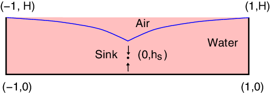
We will consider two problems for withdrawal into a line sink beneath an interface. In the first, we will allow a compensating recharge to reduce net flow to zero, thus allowing a steady solution, while, in the second we will consider the full unsteady problem and ultimate drawdown of the interface. The physical plane is shown in Figure 1. A layer of freshwater with depth
 $H^*$
occupies a homogeneous and isotropic porous medium of constant permeability,
 $\kappa$
, above a bottom boundary of impermeable rock. We may place a line sink at a distance
 $H_s$
above the bottom. For the flow to be steady, there must be recharge through the surface exactly matching flow out through the sink. Darcy’s law [Reference Bear2,Reference Darcy5] is valid, so the discharge velocity for two-dimensional flow can be expressed as
 \begin{equation}q_x=\ -K \frac{\partial \phi}{\partial x}, \ \ q_y=\ -K \frac{\partial \phi}{\partial y}.\end{equation}
The hydraulic conductivity is
 $ K= \rho g \kappa /\mu$
, where
 $\kappa$
is permeability,
 $\rho$
is density, g is gravity and
 $\mu$
is viscosity, and
 $\phi=p/\rho g +y$
is the piezometric head. In this formulation, the potential within the domain must satisfy the continuity equation
 \begin{equation}\nabla \cdot \bf q = 0,\end{equation}
and this combined with Darcy’s law requires that we satisfy Laplace’s equation for
 $\phi$
, i.e.
 \begin{equation}\nabla^2\phi=0, -L<x<L, 0 < y < S(x, t),\end{equation}
where
 $y=S(x, t)$
is the equation of the (unknown) surface of the saturated zone. There is a line sink at
 $(0, H_s)$
, so that the piezometric head behaves as
 \begin{equation} \phi \to \frac{m_0}{2\pi K} \log \left(x^2+(y-H_s)^2)\right)^{1/2} \quad \mbox {as} \quad (x, y) \to (0,H_s),\end{equation}
where
 $m_0$
is the strength of the sink. Therefore, if
 ${V}_{0}\,=\,2{m}_{0{L}}$
is the speed of the recharge at the interface the flux into the sink is
 $Q=m_0$
, matching the flux through the top.
Definition sketch for the problem. In nondimensional variables, the surface is
 $y=\eta(x,t)$
with height H at
 $x=\pm1$
. The sink is situated at
 $y=h_s$
, and in the steady problem there is recharge through the free surface.

There can be no flow through the impermeable boundaries at
 $x=\pm L$
, and invoking the left-right symmetry of the flow we can write
 \begin{equation} \phi_x(0, y, t)=\phi_x(L, y, t)=0 \mbox{ on } y<S(x, t),\end{equation}
and only consider the region
 $0<x<L$
. In this half region, the volume flux into the sink is
 $\frac{m_0}{2}$
. Now, since the pressure on the free boundary is constant, the piezometric head equation can be written
 \begin{equation} \phi(x,S(x, H))=S(x,t),\ \mbox{ on } y=S(x, t),\ 0< x < L.\end{equation}
Finally, water particles on the free surface must remain on the surface, leading to the kinematic condition, which in terms of
 $\phi$
becomes
 \begin{equation}S_t-K \phi_y+K \phi_xS_x+\frac{m_{0}}{2L}=0, \mbox{ on } y=S(x, t),\ 0<x<L.\end{equation}
In this equation, the final term represents recharge at the interface if it is present. In steady flow, this is chosen to match exactly the volume of withdrawal through the line sink, thus allowing the possibility of a steady solution, while in unsteady flow we omit this term. Nondimensionalising with respect to the width L, the time scale
 $T=L/K$
and the volume flux
 $m_0$
, where the nondimensional flow speed of the recharge water is
 $ \frac{m}{2}$
, we find the equations become
 \begin{align} &\nabla^2 \phi=0,\ \mbox{ in } \ 0<x<1, \ 0<y<\eta(x, t) \end{align}
 \begin{align} &\phi_x=0, \mbox{ on } x=0, x=1,\ 0<y<\eta(x, t) \end{align}
 \begin{align} &\phi=\eta, \mbox{ on } y=\eta(x ,t), 0<x<1 \end{align}
 \begin{align}&\eta_{t}-\phi_y+\phi_x\eta_x+\frac{m}{2}= 0 \mbox{ on } y = \eta(x, t),\ 0<x<1 \end{align}
 \begin{align}&\phi(x,\eta, 0)=\eta(x, 0)=H, \mbox{ at } t=0, \end{align}
where
 $\eta(x,t)$
is the nondimensional height of the free surface,
 $y=H$
is its initial location,
 $h_s=H_s/L$
and all variables are now written in nondimensional form. As the sink is approached, the potential function
 $\phi$
behaves as
 \begin{equation} \phi \to \frac{m}{2\pi}\log\left(x^2+(y-h_s)^2\right)^{1/2} \ \mbox{ as } (x, y)\ \mbox{ to } (0, h_s),\end{equation}
where m is a nondimensional sink strength parameter,
 $m={m_0}/{K}$
. The problem is therefore to solve the system given by equations (2.8)–(2.12), subject to (2.13). Note that in this formulation, no account is taken of partially saturated flows or the capillary fringe that exist near the free surface. Modifications to the work here can be presented that do take into account such features, as was done in the work of Youngs [Reference Youngs18] for example, but as a simple model the omission of these is not an unreasonable assumption.
3 Steady flow in a duct
First, we consider steady withdrawal with a matching surface recharge. Since the flow is steady, we note the surface equation is
 $y= \eta(x)$
and that
 $\eta_{t} \equiv 0$
in (2.8)–(2.12). In order to consider this free surface problem, we seek a solution
 \begin{equation}\phi=\phi_s+\sum_{n=0}^\infty{a_n} \ {\cosh \ \lambda_n y} \ {\cos\lambda_n \ x}, \ \ \ -1<\ x\ <1\ ,\ 0\ <\ y\ <\ \eta(x),\end{equation}
where
 $\phi_s$
is a solution for flow into a sink in a vertical duct that is confined below. This choice of
 $\phi$
takes care of all boundary conditions except those on the free surface provided
 $\lambda_{n}=n \pi$
,
 $n=1,2,3\dots$
and
 $\phi_{s_{y}}=0$
on
 $y = 0$
. Defining
 \begin{equation}\eta=H+b_{0}+\sum_{n=1}^\infty \ b_n\ {\cos\lambda_n \ x}, \ \ \lambda_{n}=n\pi,\end{equation}
where
 $b_{0} = -\sum_{n=1}^\infty{b_{n}(-1)^{n}}$
, so that
 $\eta(1) = H$
, we will be able to compute the shape of the phreatic surface by satisfying the surface conditions (2.10) and (2.11), which in steady flow are
 \begin{align}&\phi=\eta, \mbox{ on } y=\eta(x), 0<x<1 \end{align}
 \begin{align}&\phi_y-\phi_x\eta_x-\frac{m}{2}= 0 \mbox{ on } y = \eta(x),\ 0<x<1. \end{align}
A powerful method of finding
 $\phi_s$
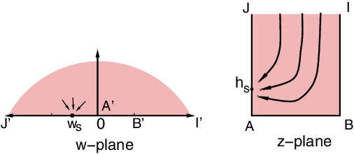
is to use conformal mapping and complex variables. We have to satisfy Laplace’s equation in the domain, and conditions of no flow through the boundary. We write the solution in the complex plane for a line sink on the boundary of the upper half plane and then map this region to the duct as shown in Figure 2. The complex function
 $F_s(w)=\phi_s+i\psi_s$
, where
 $\psi_s$
defines the streamfunction, in the upper-half w-plane, for a line sink at
 $w = -w_s$
, is
 \begin{align} F_s{(w)}&=\phi_s +i \psi_s\end{align}
 \begin{align} & =\frac{m}{2 \pi}\log(w-w_s).\end{align}
Then at the point
 $w_s$
there is a logarithmic singularity and the flow lines are radial in the w-plane. The mapping from the w to the z plane, such that the points
 $A_1,B_1,I_1,J_1$
map to A, B, I, J as shown in Figure 2, is given by
 \begin{eqnarray}w= \cos^{2} \left( \frac{\pi(1-z) }{2} \right).\end{eqnarray}
The conformal mapping of the complex z-plane to the upper half of the complex
 $w-$
plane. The points A, B, I, J in the z-plane map to corresponding point A’, B’, I’, J’ in the w-plane.

Substituting (3.7) into (3.5), we find the complex potential
 \begin{equation}F_s{(z)} = \frac{m}{2 \pi}\ \log \left(\cos^{2} \frac{\pi(z-1)}{2}\ -\ \cos^{2} \frac{\pi(z_{s}-1)}{2} \right).\end{equation}
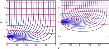
In each case, a correction to this solution will be computed that satisfies the conditions of the full problem. Examples of flow nets for this duct flow are shown in Figure 3, in which the flow lines and equipotentials are shown for sinks at (a)
 $h_s$
= 0.5 and (b)
 $h_s$
= 1.5. Note that there is very little flow deep in the column when the sink is situated well away from the base.
The equipotential (red) and streamlines (blue) for flow in a duct, with a line sink located at (a)
 $h_s$
= 0.5, (b)
 $h_s$
= 1.5.

3.1 Linear steady solution
If the flow rate is very small or the sink is a long way from the interface, then we can assume that the disturbance of
 $\eta (x)$
about
 $y = H$
is small. In nondimensional coordinates, this means that the parameter m is very small. Under that case, we can omit the nonlinear term in (3.4) and enforce conditions (3.4) and (3.3) on
 $y = H$
instead of
 $y=\eta(x)$
. Hence, these conditions become
 \begin{align} \eta&=\phi, \mbox{ on } y=H, 0<x<1 \end{align}
 \begin{align} \phi_y&= \frac{m}{2}, \mbox{ on } y=H,\ 0<x<1. \end{align}
We consider a solution to the flow from a vertical duct into a line sink as suggested above
 \begin{equation}\phi=\phi_s+\sum_{n=0}^\infty{a_n} \ {\cosh \ \lambda_n y} \ {\cos\lambda_n \ x},\end{equation}
where
 $\phi_s$
is the solution for flow into the sink in a vertical duct with no water surface as given in (3.8). Substituting into the linearised conditions (3.9), (3.10) we require
 \begin{equation}\phi_y=\phi_{sy}+\sum_{n=0}^\infty{a_n}{\lambda_n\ \sinh \lambda_n H} \ {\cos \lambda_n x} =\frac{m}{2},\end{equation}
and substituting the form (3.1) into equation (3.12) we find, using orthogonality that
 \begin{equation}a_n=\frac{1}{2} \int_0^1 \left[ \frac{m}{2}-\phi_{sy}(x,H)\ \right] \cos n \pi x\ dx, \ \ n=1,2,...\end{equation}
and then implementing
 $\eta(x)=\phi(x,H)$
gives, with
 $a_n$
given by (3.13),
 \begin{equation*}\eta =\sum_{n=0}^\infty{a_n}\ {\cosh \ \lambda_n H}\ {\cos\lambda_n \ x}.\end{equation*}
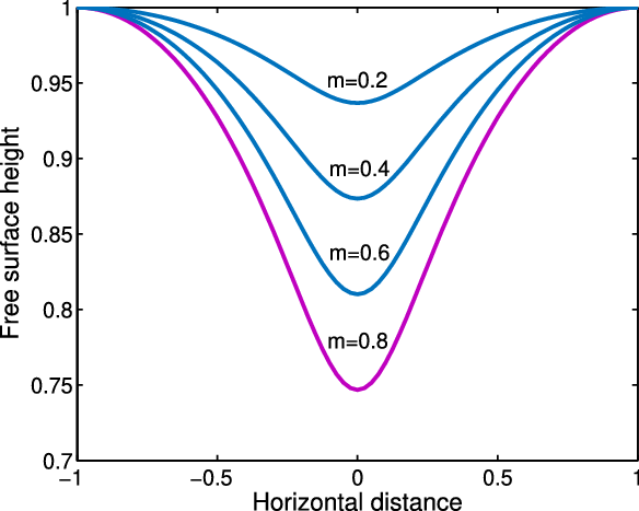
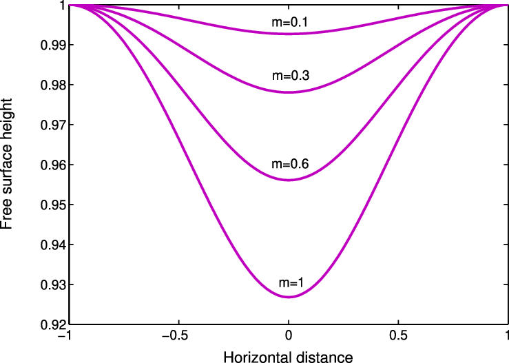
Examples of the free surface shapes for different flow rates m are shown in Figure 4 with the surface at height H =1 and depth of the sink
 $h_s=0.75$
, and with
 $h_s=0.25$
in Figure 5. As m increases, or the sink moves closer to the surface, the steady surface pulls down further in the centre.
The free surface shape of the steady, linear solution for different flow rates, m at height H = 1 and sink depth
 $h_s$
= 0.75.

The free surface depth of the steady, linear solution for different flow rates, m, at height H = 1 and sink depth
 $h_s$
= 0.25.

3.2 Nonlinear steady solution
To solve the full nonlinear steady problem, we must satisfy the conditions (3.3) and (3.4) on the actual phreatic surface
 $y = \eta(x)$
, rather than on
 $y = H$
. This invalidates orthogonality in most cases, but we can still proceed, although the resulting equations will be nonlinear.
Given the choice of
 $\phi$
in (3.11), a sensible form for the equation of the interface is the one given in (3.2), and using (3.1) and (3.2) in (3.3) then on
 $y=\eta(x)$
,
 \begin{equation}b_0\ +\sum_{n=1}^\infty{b_n}{\cos\lambda_n x}\ +H -\ \phi_s-\sum_{n=0}^\infty{a_n}\ {\cosh \lambda_n \eta}\ {\cos\lambda_n x} =0.\end{equation}
Multiplying all terms by
 $\cos \lambda_j x$
and integrating from 0 to 1 give
 \begin{align}&\sum_{n=1}^\infty{b_n}\int_{0}^{1} \ {\cos \lambda_n x} \ {\cos \lambda_j x} \ dx\ + \ H \ \int_{0}^{1} \ {\cos \lambda_j x} \ dx -\ \int_{0}^{1} \frac{m}{2 \pi} \ {\log \ R \ {\cos \lambda_j x}} \ dx \nonumber \\ &\quad -\sum_{n=0}^\infty{a_n}\int_{0}^{1} \ {\cosh \lambda_n \eta} \ {\cos\lambda_n x} \ {\cos \lambda_j x} \ dx = \ 0,\end{align}
where
 $R=(x^2+(\eta-h_s)^2)^{1/2}$
. Similarly for the dynamic condition (3.4), we note
 \begin{equation}\phi_y=\phi_{s_y}+\ \sum_{n=0}^\infty{a_n}\ \lambda_n\ {\sinh \lambda_n} {\eta}\ {\cos \lambda_n x} \ \ \mbox {when} \ \ y=\eta(x),\end{equation}
 \begin{equation}\eta^\prime(x)=-\sum_{n=0}^\infty{b_n} \lambda_n \ {\sin\lambda_n x}\end{equation}
and
 \begin{equation}\phi_x=\phi_{s_x}-\ \sum_{n=0}^\infty{a_n} \lambda_n\ {\cosh \lambda_n} {\eta}\ {\sin \lambda_n x}.\end{equation}
Combining (3.16), (3.17) and (3.18) in (3.4) gives
 \begin{align} \phi_{s_y}\ +\ \sum_{n=0}^\infty{a_n} (\lambda_n \ {\sinh \lambda_n}\ {\eta}\ {\cos\ \lambda_n \ x} \ + \frac{m}{2})\ -\ \phi_{s_x}\ \left( -\sum_{n=0}^\infty{b_n} \ {\lambda_n } \ {\sin \lambda_n x} \right)\\ -\ \left( \ \sum_{n=0}^\infty{a_n}\ {\cosh \lambda_n\ \eta} \ {\lambda_n }\ {\sin\lambda_n\ x} \right) \left( -\sum_{n=0}^\infty{b_n} \ {\lambda_n } \ {\sin \lambda_n x} \right) =0 \end{align}
and again integrating (3.19) from zero to one after multiplying (3.19) by
 $\cos \lambda_j x$
gives
 \begin{align}&\int_{0}^{1} \phi_{s_y} \cos \lambda_j x\ dx +\sum_{n=0}^\infty{a_n} \int_{0}^{1} \left( \lambda_n \ {\sinh \lambda_n} {\eta}\ {\cos \lambda_n x}+ \frac{m}{2} \right) \cos \lambda_j x\ dx\\&\quad+\int_{0}^{1} \left( \left( \phi_{s_x}+\sum_{n=0}^\infty {a_n}{\lambda_n }\ {\cosh \lambda_n \eta} \ {\sin\lambda_n x}\right) \left( \sum_{n=0}^\infty{b_n} {\lambda_n } \ {\sin \lambda_n x}\right) \right) \cos \lambda_j x\ dx =0,\\ &\hspace{275pt}\mbox{ for } j=1, ..., \infty. \end{align}
To compute the numerical values of the free surface,
 $\eta(x)$
, the fsolve routine in MatlabTM for nonlinear systems of equations was used. We truncate the two series after N terms, giving 2N unknowns. Multiplying by
 $\cos \lambda_n x$
and integrating over 0 to 1 for
 $n = 1, 2,.., N$
in (3.15) and (3.20) gives 2N equations to solve with MatlabTM for the 2N unknown coefficients
 $a_n$
and
 $b_n$
for
 $n = 1,..., N$
.
3.3 The results
A series of computations was performed for different values of m and H. Results of the two-dimensional finite depth problem give that the deepest point on the surface gets lower as the pumping rate increases as expected and as was shown in the linear solutions.
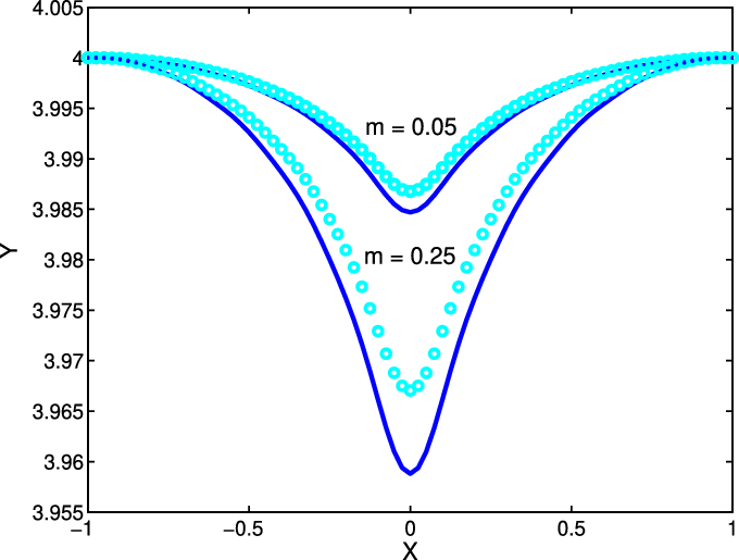
Figure 6 shows a comparison of the steady solution with the solution to the approximate, linearised equations with reasonable agreement when H = 4 and
 $h_s = 3.9$
with withdrawal rates
 $m = 0.05$
and
 $m=0.25$
. The comparison is quite good for the smaller value of m, and not quite so good when
 $m=0.25$
, as might be expected. For values of
 $m<0.05$
(not shown), agreement is very good. The linear solutions do not draw as far down because of the evaluation of the terms on
 $y=H$
rather than
 $y=\eta(x)$
. Thus, the nonlinearity manifests as a deeper cone shape.
Steady free surface with sink at
 $h_s$
= 3.9, H = 4 for m = 0.05, 0.25. The circles indicate the equivalent linear solutions.

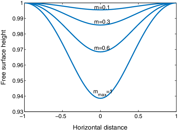
Figure 7 shows the shape of the interface for increasing values of m when
 $H = 1$
and
 $h_s = 0.25$
. For each value of H, it was found there was a maximum value of flow rate m beyond which no steady solutions were found. In this case, no steady solution seems to exist for
 $m > 1$
.
Steady free surface depth at height
 $H = 1 $
with depth of sink
 $h_s = 0.25$
. In this case, no steady solution seems to exist for
 $m > 1$
.

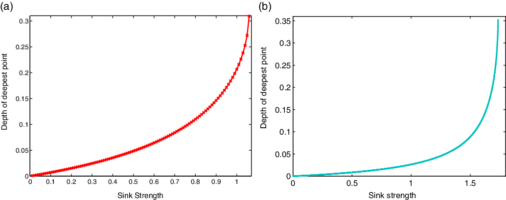
Figure 8(a) and (b) shows the relation between the deepest point and the value of the pumping rate m at fixed surface height
 $H = 1$
,
 $h_s=0.2$
and
 $H = 2$
,
 $h_s=0.75$
, respectively. It is clear that as m increases the depth of the deepest point increases rapidly as
 $m_{\max}$
is approached.
The relationship between sink strength m and the deepest point on the free surface in a steady state at (a) H = 1 and
 $h_s$
= 0.25, for which
 $m_{\max}\approx 1.07$
, and (b) H = 2 and
 $h_s$
= 0.75 where
 $m_{\max} \approx 1.735$
. The depth rapidly increases as it approaches the limiting m value.

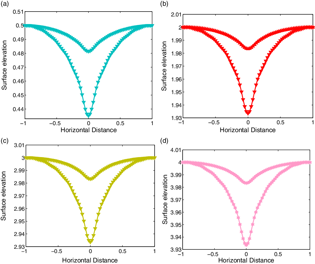
We have studied the situation at different surface elevations to determine the effect of sink elevation. For example, Figure 9 shows free surface shapes
 $y = \eta(x)$
for different total depth H when the sink is submerged so that
 $H-h_s=0.1$
, i.e. the sink is relatively close to the surface. The shapes are almost identical when the sink strengths are the same. It is clear as
 $h_s$
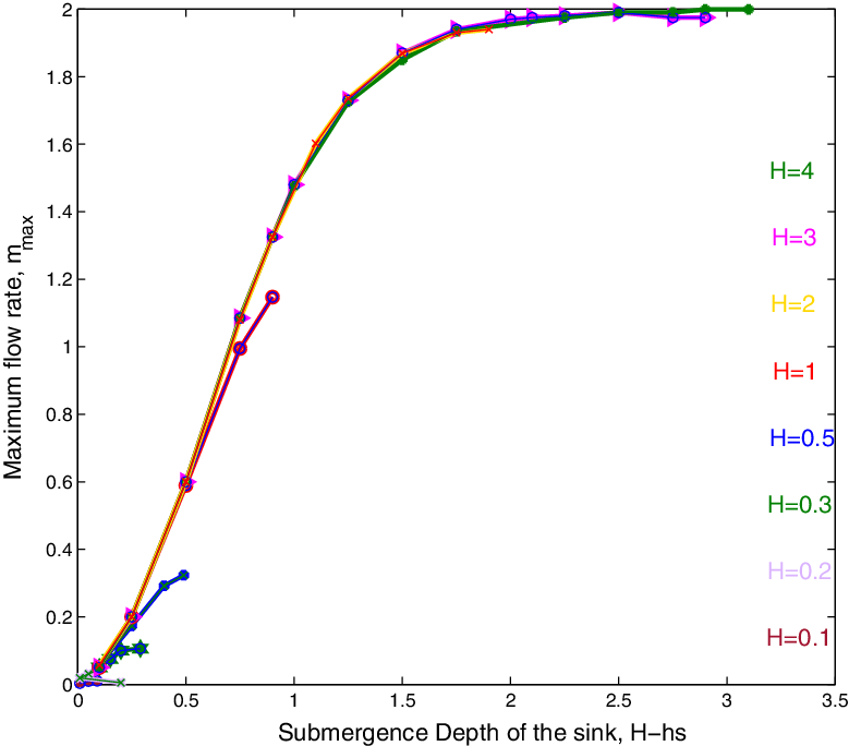
increases the effect of the bottom begins to diminish and the flow is mainly dependent on the distance between the sink and the interface. This is verified in Figure 10 which shows the relationship between the submergence depth and the maximum rate
 $m_{\max}$
for different surface heights H. Except for small values of H, the maximum values become aligned. This strong alignment confirms that it is the submergence depth that is the primary factor in determining the critical withdrawal unless the sink is close to the bottom. As H increases, there seems to be an absolute maximum flow rate of
 $m_{\max} \approx 2$
, so long as the sink is not too close to the base.
The nonlinear surface shape for the same submergence depth for (a) H = 0.5,
 $h_s$
= 0.4, (b) H = 2,
 $h_s$
= 1.9, (c) H = 3,
 $h_s$
= 2.9, (d) H = 4,
 $h_s$
= 3.9 with withdrawal rates m = 0.025, 0.05. Note the vertical scales are the same but the top point in each case differs.

The maximum withdrawal rate
 $m_{\max}$
with sink submergence
 $H-h_{s}$
for different heights, H. For larger H and
 $h_s$
, the maximum m value is close to
 $m_{\max}\approx 2$
.

If the distance between the sink height
 $h_s$
and the surface height H is large, then a greater flow rate m is required to pull down the interface. The presence of the base restricts the inflow slightly, making the sink appear slightly ‘stronger’ and causing the coning to occur at slightly lower flow rates. However, once the sink moves away from the base the flow restriction no longer occurs and the base has minimal impact.
4 Unsteady flow
We have obtained solutions to the steady problem in the confined column by allowing a matching recharge flow. However, in general, the flow will be unsteady, and so in this section, we consider the unsteady flow problem. We can use the same general approach as the steady problem but allow the series coefficients to be functions of time. To solve the full equations, we need to satisfy all of the surface conditions on
 $y = \eta(x, t)$
, and the coefficients are functions of time. In the unsteady problem, we will omit the surface recharge.
Time variation can be determined via equation (2.11). Differentiating the now time-varying version of
 $\eta$
gives
 \begin{equation}\eta_{t}(x,t)=b^{\prime}_{0}(t)+\sum_{n=1}^\infty{b_{n}^{\prime}(t)}\ {\cos(\lambda_n x)}, \ \lambda_n=n\pi.\end{equation}
Now the algorithm uses (2.10) and substituting into (2.11) and using orthogonality where appropriate, we find
 \begin{align}&b^{\prime}_{0}(t)=\int_{0}^{1} \phi_{s_y}\ dx +\ \sum_{n=0}^\infty{a_n} \int_{0}^{1} \left( \lambda_n \ {\sinh \lambda_n}\ {\eta}\ {\cos\ \lambda_n \ x} \ + \frac{m}{2} \right) \ dx\\&\qquad\qquad -\ \int_{0}^{1} \left( \left( \phi_{s_x}\ +\ \sum_{n=0}^\infty{a_n}\ {\cosh \lambda_n\ \eta} \ {\lambda_n }\ {\sin\lambda_n\ x} \right) \left( -\sum_{n=1}^\infty{b_n} \ {\lambda_n } \ {\sin \lambda_n x} \right) \right)\ dx\end{align}
and
 \begin{align}\frac{1}{2} b^{\prime}_{j}(t)&=\int_{0}^{1} \phi_{s_y}\ \cos \lambda_jx\ dx +\ \sum_{n=0}^\infty{a_n} \int_{0}^{1} \left( \lambda_n \ {\sinh \lambda_n}\ {\eta}\ {\cos\ \lambda_n \ x} \right) \ \cos \lambda_jx\ dx \nonumber\\ &\quad -\ \int_{0}^{1} \left( \left( \phi_{s_x}\ +\ \sum_{n=0}^\infty{a_n}\ {\cosh \lambda_n\ \eta} \ {\lambda_n }\ {\sin\lambda_n\ x} \right) \left( -\sum_{n=0}^\infty{b_n} \ {\lambda_n } \ {\sin \lambda_n x} \right) \right)\ \cos \lambda_jx\ dx .\end{align}
The values of
 $b_j(t), j=1, 2,\dots, N$
are then updated simultaneously with the dynamic condition in the form of (3.14), (3.15) to find the new values of
 $a_j(t), j = 1, 2, \dots$
using a 4th-order Runge–Kutta scheme.
At
 $t = 0,\ \eta = H,$
and
 $b_j(0) = 0;\ \ j=1, 2,..., N$
, so invoking orthogonality at this initial time,
 \begin{eqnarray}a_j(0)=-2 \int_{0}^{1} \ {\phi_s{(x,H)}} \cosh (\lambda_j H) \ {\cos\lambda_j \ x} \ dx,\end{eqnarray}
are the initial values for
 $j=1, 2, 3, \dots, N$
. H(t) is again the height of the free surface at x = 1.
4.1 Linear unsteady solution
As in the steady solution, we can obtain a linear solution by assuming that the product terms in (2.11) are small. If the deviation of the surface is small, then we can find the coefficients by linearising about the average surface height at each step, and evaluating all equations on
 $y = H(t)$
i.e.,
 \begin{equation}\eta_{t} =\ -\phi_{y}(x,y), \ \ \mbox {evaluated on} \ \ y = H(t).\end{equation}
Substituting the series forms for
 $\eta$
and
 $\phi$
into this equation gives that the height of the water surface can be obtained from
 \begin{align} b_0^\prime(t)\ +\ \sum_{n=0}^\infty {b_n}^\prime\ {\cos \lambda_n x} &= - \frac{1}{2}\ \sum_{n=0}^\infty {a_n} \lambda_n\ (e ^{\lambda_{n}(y-b_{0})} \ +\ b \ e ^{-\lambda_{n}(y+b_{0})})\ \cos \lambda_{n}x \nonumber\\ &\quad - \phi_{sy}(x,b_{0}).\end{align}
Now since the coefficient of
 $\cos \lambda_{n}x$
is constant for each term, we can invoke orthogonality to find an integral expression for each of the coefficients as
 \begin{equation}b_{j}^\prime(t)=-2\ \int_{0}^{1}\ \phi_{sy}(x,b_{0})\ \cos\ \lambda_{j}\ x\ - a_j(t), \ j=1, 2,..., N.\end{equation}
We can then compute
 $a_j (t)$
using (2.10), so
 \begin{eqnarray} a_{0}(t) =b_{0}(t) - \int_{0}^{1}\ \phi_s (x,b_{0}(t) )\ dx\end{eqnarray}
and
 \begin{eqnarray} a_j (t)=b_{j}(t) -\ 2 \int_{0}^{1}\ \phi_s (x,b_0 )\ \cos \lambda_j x\ dx.\end{eqnarray}
Once we have obtained
 $b_{j}(t)$
we can update the phreatic surface using
 $\eta(x,t)$
from equation (4.1). In these calculations, all of the coefficients can be computed ‘exactly’ at each step.
4.2 Nonlinear unsteady solution
In the nonlinear problem, we have the same steps as for the linear, but we must now evaluate the equations on
 $y=\eta(x,t)$
rather than
 $y=H(t)$
. We now need to step in time, so need to find
 $\frac{db_n}{dt}$
using
 \begin{eqnarray} \eta_t = b_0^\prime(t)+\sum_{n=0}^\infty{b_n^\prime(t)}\ \cos \lambda_n x\ =\ \phi_{x} \eta_{x}\ -\ \phi_{y}\end{eqnarray}
where the right-hand side is given by the appropriate series (3.16), (3.17), (3.18) and all terms are evaluated on
 $y=\eta(x,t)$
. Using orthogonality as appropriate, and if we know
 $a_n$
and
 $b_n$
for
 $n = 1, 2,..., N$
, we can find
 $\frac{db_n}{dt}$
as follows:
 \begin{equation} b_n^\prime(t)=2\ \int_{0}^{1} \ (\phi_{x} \eta_{x}\ -\ \phi_{y})\ {\cos\lambda_n x} \ dx.\end{equation}
The values of
 $b_{n}(t), n = 1, 2,..., N$
are then updated simultaneously with the dynamic condition in the form of (4.10), (4.11) and (3.14), (3.15). To find new values of the coefficients
 $a_{n}(t), n=1,2,...$
we use fsolve at each sub-step of the 4th-order Runge–Kutta scheme.
4.3 Results and comparison
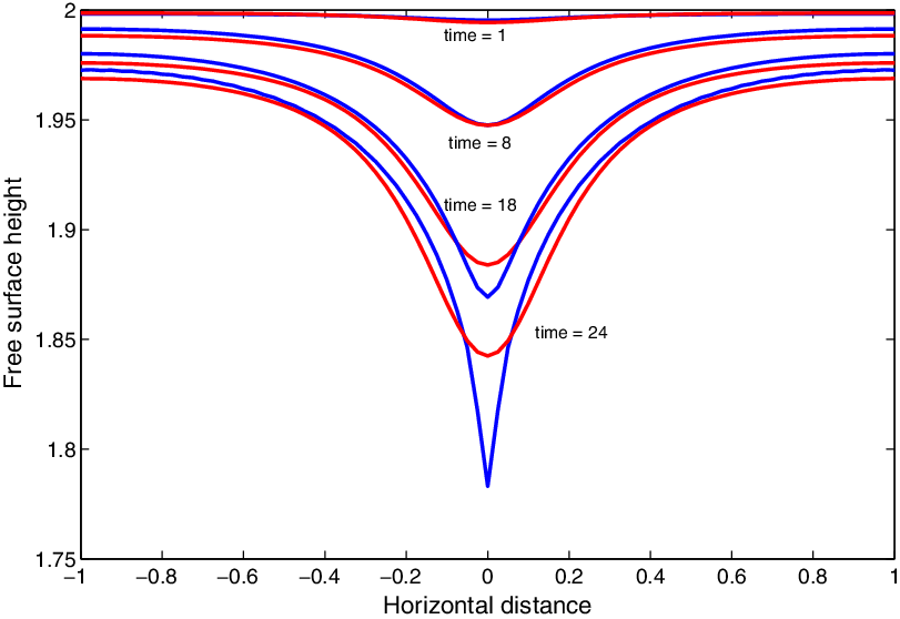
Figure 11 shows a comparison between linear and nonlinear flow solutions for initial elevation H = 2, sink depth
 $h_s$
= 0.25 and flow rate m = 2, with 40 coefficients. At early times, the two agree very well, but as the surface gets more distorted, the nonlinearity causes the middle of the surface to travel downward faster. As time proceeds, the central point accelerates downward, signifying that coning is about to occur. In the nonlinear calculations, the method breaks down as the point of coning is reached as the surface accelerates, and so the middle point cannot be tracked completely into the sink.
The free surface shape of the linear (red) and the nonlinear (blue) when the distance between the initial elevation and the sink is 1.75 and m = 2 with 40 coefficients.

As we saw in Section 3.3, the most important factor determining the behaviour of the interface in both the linear and nonlinear cases is the location of the sink relative to the surface. The distance from the outer edge of the free surface H(t) to the sink
 $h_s$
at the moment of coning represents a critical height
 $\eta^{*}=\eta(1,t_{crit})-h_s$
, where
 $t_{crit}$
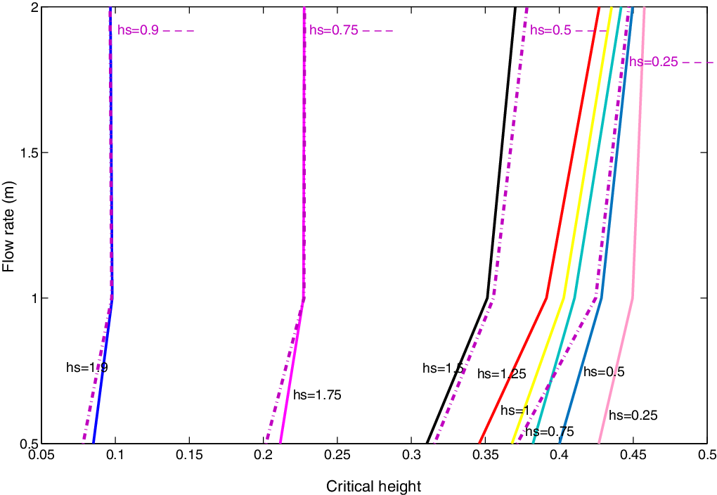
is the time of coning. This height is significant because in a wide aquifer it is this height that would be monitored and so as it was approached drawdown would be imminent. The distance to this line is the critical height,
 $\eta^{*}$
, for each m. As m increases, the drawdown occurs sooner and so
 $\eta^{*}$
is larger. The highest and lowest points on the surface depend on the value of m for different locations of the line sink
 $h_s$
.
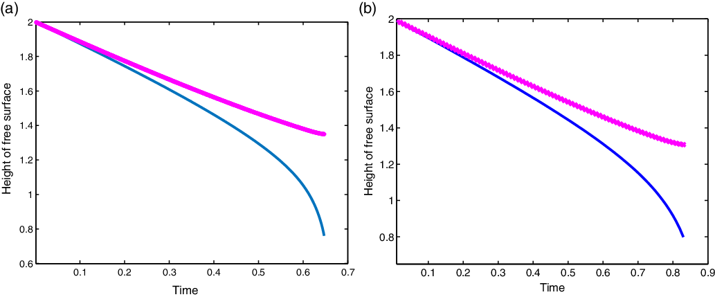
Figure 12 shows the highest and lowest points on the free surface, at the outer edge and middle, respectively, as a function of time. Once the surface pulls down, the water above the interface will also flow into the sink. Interestingly, the coning occurs in both cases when the outer level of the interface reaches
 $\eta(1,t_{crit})\approx 1.35$
.
The highest and lowest points on the free surface of the nonlinear solution, with
 $H=2, h_s=0.75$
; (a) with
 $m = 2.4$
the code breaks down as the surface accelerates at
 $t = 0.647$
,
 $\eta(1) \approx 1.35$
. (b) with
 $m=2$
breakdown at time
 $t\approx 0.87$
, the code breaks down as the surface accelerates at t = 0.83,
 $\eta(1) \approx$
1.35.

In cases where m is large and
 $H-h_{s}$
is small, the drawdown or coning is almost immediate. When the flow rate m is smaller, the lowest point will take much longer to draw down. The probable reason for the failure of the numerical method in the simulations can be seen in Figure 12(a), (b), which shows that the middle of the interface moves downward extremely fast, becoming essentially singular in time.
Figure 13 shows the value of
 $\eta^{*}$
when the drawdown occurs. For a particular sink elevation and initial surface elevation, the central cone is pulled down faster as flow rate m increases, leading to larger values of the critical height. When the submergence of the sink is small, the value of the critical depth is almost independent of H for different flow rates m, but when the sink is closer to the bottom, the critical value is more strongly affected by the flow rate m. The results suggest that as in the steady case the main factor in determining the critical withdrawal, unless the sink is close to the bottom of the region, is the submergence depth. Therefore, for cases where the sink is not close to the base, the behaviour of the surface will be almost identical if m and the submergence depth
 $H-h_s$
are the same, independent of the total depth H.
The critical height
 $\eta^{*}$
for starting heights
 $H = 1$
(dashed line) and
 $H=2$
(solid line) for different values of sink location
 $h_s$
versus the flow rate.
 $H=2$
has extra cases for when sink is above 1.

5 Comsol multiphysics software package
As further verification of the results described above, simulations were performed in the COMSOLTM Multiphysics modelling package. The subsurface flow module extends the COMSOLTM modelling environment to enable consideration of fluid flow in saturated and variably saturated porous media [Reference Mozafari, Fahs, Ataie-Ashtiani, Simmons and Younes14]. The velocity field is determined by the pressure gradient, the fluid viscosity and the structure of the porous medium according to Darcy’s law. The gradient in hydraulic potential drives fluid movement in the porous medium. In this paper, we will use the notation and dimensional formulation used in the COMSOLTM package, but chosen to be directly comparable to the parameters in the earlier sections. According to Darcy’s law, the net flux is
 \begin{equation}u=-\frac{\kappa}{\mu}(\nabla p+ \rho \nabla gz),\end{equation}
where u is specific discharge vector or the Darcy velocity (m/s),
 $\kappa$
is the permeability of the porous medium (m
 $^2$
),
 $\mu$
is the fluid dynamic viscosity (Pa.s), p is the fluid pressure (Pa),
 $\rho$
is density (kg/m
 $^3$
) and
 $\nabla z$
is a unit vector in the direction in which the gravity acts. Models can define the capacity to transmit flow using the permeability of the porous medium,
 $\kappa$
, and the viscosity of the fluid,
 $\mu$
, or using the hydraulic conductivity, K (m/s) where
 $K=\frac{\kappa \rho g}{\mu}$
.
The hydraulic conductivity combines properties of both the fluid and porous matrix, while the permeability is a property of the porous matrix only. The hydraulic potential in the equation comes from the pressure, p, and gravity,
 $\rho g z$
. The mass transport equation is
 \begin{equation}\frac{\partial}{\partial t}(\rho \varepsilon) + \nabla . \rho u= Q_m,\end{equation}
where
 $\rho$
is the fluid density (kg/m
 $^3$
),
 $\varepsilon$
is the porosity and
 $Q_m$
is a mass source term (kg/(m
 $^3$
s)). Porosity is the fraction of the control volume that is occupied by pores. Substituting (5.1) into the continuity equation (2.2) and then defining the porosity and the density as functions of the pressure, and applying the chain rule gives
 \begin{equation}\varepsilon \frac{\partial \rho}{\partial t} +\rho \frac{\partial \varepsilon}{\partial t} = \varepsilon \frac{\partial \rho}{\partial p} \frac{\partial p}{\partial t} + \rho \frac{\partial \varepsilon}{\partial p} \frac{\partial p}{\partial t}.\end{equation}
The subsurface flow module can be used to consider problems with variable soil and water properties, but in this work we will focus on homogeneous and uniform situations to compare with the spectral method.
5.1 Two-dimensional confined vertical duct
We set up COMSOLTM to compare with the results of the unsteady spectral method in which we considered withdrawal through a line sink in a vertical drain confined below. As above, we consider a two-dimensional sand column, and neither flow through the bottom nor the two vertical sides were allowed. There are two layers of different density separated by an interface. However, there is flux coming down from the top into the upper layer and the lower layer flows into a line sink, which is situated on the line x = 0 above the bottom at different heights
 $h_s$
to determine the effect of sink elevation on the behaviour of the interface. The unknown interface will be symmetric about x = 0. The flux from the top does not cross the interface and so simply serves to replenish the water in the top layer. It is the behaviour of the interface that is of interest.
The outflow mass flux
 $q_a$
in COMSOLTM and flux m from the spectral method are related by the formula
 $q_a = \frac{\varepsilon \rho m}{2}$
. The values used for the different parameters are given in the table in the Appendix.
5.2 Comparison with COMSOLTM
The results above were compared with simulations using the computer package COMSOLTM. COMSOLTM is formulated in a dimensional frame of reference, and so we used dimensional parameters that matched the choices of nondimensional parameters given above. Computations were performed for different values of mass flux,
 $q_a$
, at an initial height H and sink heights pt1, which correspond to heights
 $h_s$
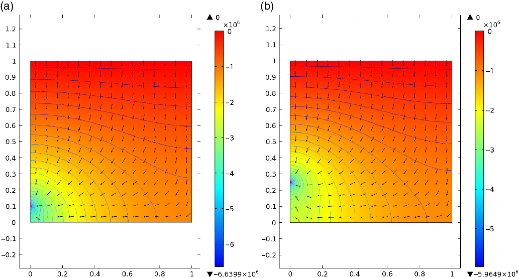
. In Figure 14, the contours of pressure and vector fields were computed when the initial height H = 1 and the flux mass volumes m = 1.383 and m = 2 at sink locations
 $h_s$
= 0.1 and
 $h_s$
= 0.25.
Contours of pressure and the flow vectors at initial height H = 1 when (a) the flux mass volume m = 1.383 and the sink location
 $h_{s}$
= 0.1, (b) the flux mass volume m = 2 and the sink location
 $h_s$
= 0.25.

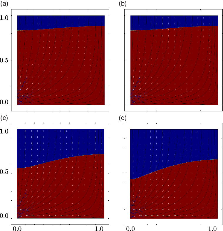
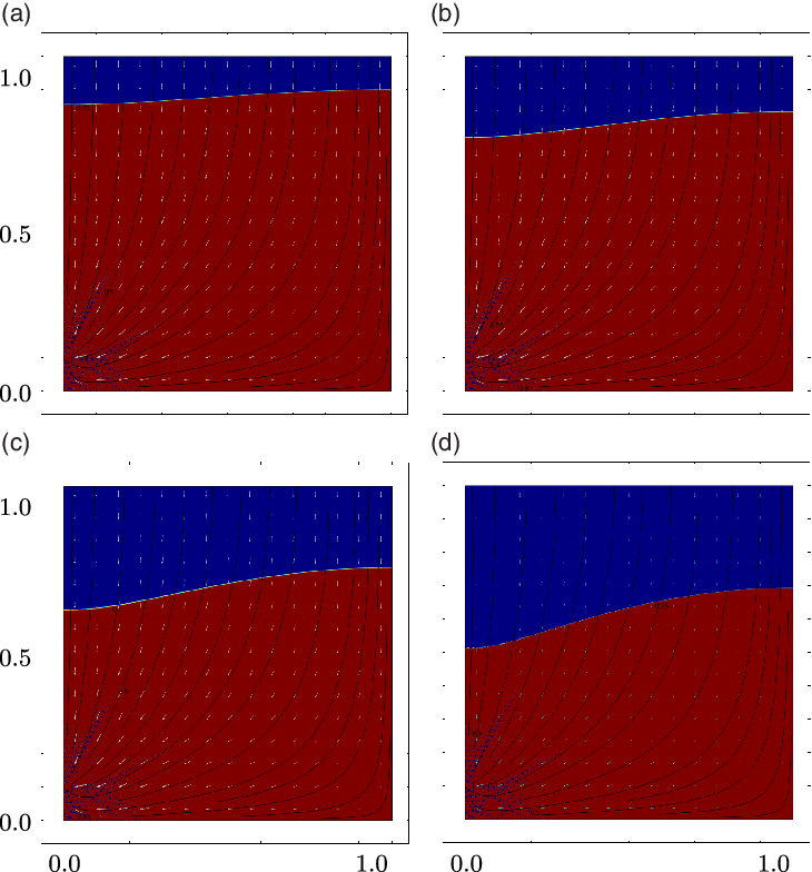
Some results of the interface, contours and streamlines with the velocity field vectors are shown in Figures 15 and 16. Figure 15 shows a sequence where the interface is drawing down into a cone starting with an initial height H = 1, and the line sink situated at
 $h_s =0.1$
with the outflux mass value
 $m = 1.383$
at different times, while Figure 16 shows the same but with a higher value of flow,
 $m=2$
. The drawdown of the interface happens at a much earlier time when the flow is stronger.
The interface, streamlines (black lines) and the gradient of the pressure (white vectors) at initial height H = 1 and the sink location
 $h_s$
= 0.1 with the outflux mass value m = 1.383 at times t = 20, 30, 50, 61.

The interface, streamlines (black lines) and the gradient of the pressure (white vectors) at initial height H = 1 and sink depth
 $h_s$
= 0.1 with the outflux mass value m = 2 at times t = 12, 20, 30, 38.

Comparison of the highest and lowest points on the free surface related to time steps in COMSOLTM (dashed line) and the spectral method (solid line). The initial height
 $H =L$
= 1, and the sink location
 $h_s$
= 0.1 with same flow rate for both models
 $q_a = \frac{\varepsilon \rho m}{2} $
= 0.4998.

The critical height
 $\eta^{*}-h_s$
versus time at height H = 1 and the sink location
 $h_s$
= 0.1 for the same flow rate for COMSOL (dashed line) and the spectral method (solid line) with
 $q_a = \frac{\varepsilon \rho m}{2}$
= 0.4998.

Comparison of the highest and lowest points on the free surface related to time steps in COMSOLTM (dashed line) and the spectral method (solid line). The initial height H = 1, and the sink location
 $h_s$
= 0.25 with same flow rate for both models
 $q_a = \frac{\varepsilon \rho m}{2} $
= 1.

The critical height
 $\eta^{*}$
versus time at height H = 1 and the sink location
 $h_s = 0.25$
for the same flow rate for COMSOL (dashed line) and the spectral method (solid line) with
 $q_a = \frac{\varepsilon \rho m}{2} = 1$
.

The surface starts horizontally but then begins to dip over the location of the exit point, gradually deepening until it appears to reach the vicinity of the sink. In the region close to the sink in the COMSOLTM model, there appears to be considerable ‘mixing’ of the two fluids of different density, probably due to the very high velocity generated by the sink point. This is happening when the value of m is large, and the ‘mixing’ decreases when the m value is reduced. This mixing of the two layers makes it difficult to determine exactly when the interface ‘enters’ the sink.
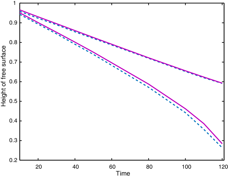
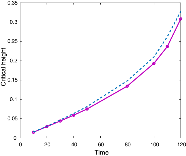
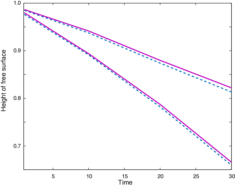
We compared some of the spectral method and COMSOLTM results for the same cases. The first comparison was for the highest and lowest points on the interface related to time for COMSOLTM with the same points on the free surface for the spectral method. The time scales for the spectral method and COMSOLTM code are different, and these have been moderated to coincide.
Both COMSOLTM and the spectral method had difficulty in accurately simulating the moments leading up to the interface entering the sink. In the spectral method, the series was unable to resolve the rapid variation in the interface shape, while in COMSOLTM there seemed to be an extreme and unrealistic amount of mixing of the fluid above and below the interface due to the very high velocities generated close to the outlet. However, comparison of the important parameters between the two methods showed that both give very similar results. Computations were performed for initial height H = 1, and the sink location
 $h_s $
= 0.1 with the same flow rate value in both versions
 $q_a = \frac{\varepsilon \rho m}{2}$
= 0.4998. The free surface drops down at time
 $t \approx 120$
and the COMSOLTM code breaks down as the surface accelerates at t = 125. The similarity of the computations of both methods is clear through Figure 17 and 19 (with
 $h_{s} = 0.25, q_{a} = 1$
), with the two interface locations remaining almost identical throughout.
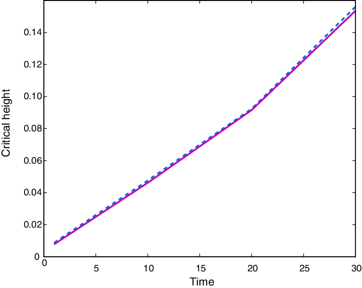
The other comparison was of the critical height
 $\eta^{*}$
versus time for cases with initial height
 $H = 1$
and sink location
 $h_s = 0.1 $
for the same flow rate for both models
 $q_a = \frac{\varepsilon \rho m}{2} = 0.4998$
as shown in Figure 18, and for another case in Figure 20 with
 $h_{s} = 0.25, q_{a} = 1$
. Again the comparison shows good agreement between the COMSOLTM solution and the MatlabTM spectral solution. Therefore, the spectral method and COMSOLTM simulation produce very similar qualitative and quantitative results. In all of the cases that we considered with both the spectral method and the finite volume method of COMSOLTM there was a strong correlation between the interface shapes and the timing of the withdrawal coning. This provides excellent validation of the results for the two-dimensional drain.
6 Conclusion
Coning of an interface during withdrawal is a well-studied subject in porous media flows. Understanding this process is essential as it relates to important issues of water quality in stratified aquifers and oil recovery in the presence of water and natural gas. We have considered such flows in an elementary, two-dimensional, sand column. Exploiting the geometry, a spectral method is formulated that can be used to solve both the steady and unsteady problems. The technique is to compute the solution for a line sink in a vertical duct and then use Fourier techniques to correct for the nonlinear surface conditions. Steady and unsteady solutions were found in both linearised and nonlinear formulations with good agreement.
It is important to note that as the aquifer is of finite dimension, then drawdown is inevitable if there is no recharge. The effects of the sink position relative to both the surface and bottom boundaries were analysed. The maximum withdrawal rate
 $m_{\max}$
for different sink depths was found. In general, if the flow rate is larger, the critical depth is larger, but as the sink gets closer to the base, the critical flow rate decreases slightly.
The important length scale in determining coning is the distance from the sink to the interface. Perhaps one of the most important result is shown in Figure 10 which shows the maximum flow rate for different sink heights, but plotted against the distance of the sink from the interface. The strong alignment suggests that this distance is the main factor in determining the critical withdrawal unless the sink is close to the bottom. If the sink is well away from the impermeable base, then it appears that the maximum flow rate is
 $m_{\max} \approx 2$
.
The spectral method and COMSOLTM can be accurate instruments for simulation of this kind of flow. The spectral method is limited to homogeneous media but can be adapted to consider cases with a capillary fringe or other interfacial conditions. COMSOLTM can be used for much more complicated media. The value of conformal mapping and spectral solutions is in their relative simplicity and in developing an understanding of the process, while the finite element techniques in COMSOLTM can be used to extend this understanding to non-homogeneous media situations. The techniques are not limited to withdrawal flows but can be used for any situation with a free surface or interface, and the spectral techniques provide an alternative to the more traditional methods of boundary element methods such as presented in Mi and Jiang et al. [Reference Mi, Jiang, Li, Li and Tian13].
Conflict of interest
None of the authors has a conflict of interest in this work.
Appendix A. Table of COMSOL values