





1 Introduction
Understanding how interpersonal relationships form and evolve in classroom settings is central to research in education, developmental psychology, and the social sciences more broadly. Early peer relations shape academic engagement, emotional well-being, and longer-term social trajectories, making classrooms a natural laboratory for studying emerging social structure. Empirical studies of classroom networks have therefore long focused on relational dimensions such as familiarity—who knows whom—and liking—who evaluates whom positively—as foundational components of peer systems.
The relationship between familiarity and liking is complex. The two are often treated as closely related. Specifically, familiarity reflects the extent to which a rater knows a ratee. According to Duck’s (Reference Duck1977) filtering model, increased familiarity facilitates the perception of shared characteristics and interpersonal similarity (Funder & Colvin, Reference Funder and Colvin1988; Hayes & Dunning, Reference Hayes and Dunning1997). Such similarity has long been regarded as an important basis of interpersonal attraction (Byrne, Reference Byrne1971), ultimately fostering liking.
An alternative perspective suggests an even stronger connection between the two constructs. Familiarity has been conceptualized as a broader relational experience comprising cognitive, affective, and behavioral components (Rockett & Okhuysen, Reference Rockett, Okhuysen and Sondak2002). From this perspective, liking is not merely a consequence of familiarity but may represent one of its core components. Consequently, familiarity and liking may reflect different manifestations of a common underlying social bond.
Taken together, these perspectives provide competing expectations regarding the relationship between familiarity and liking. Whether familiarity and liking should be represented as distinct but interdependent relational dimensions or as manifestations of a common underlying social relationship therefore remains an empirical question.
In practice, researchers, however, frequently rely on descriptive network summaries or analyze each relation separately, implicitly assuming that these relations either reflect a single underlying social dimension or differ only in degree. At the same time, classroom network data are inherently complex: relationships are directional, ratings are often ordinal rather than binary (Freeman, Reference Freeman1984), and multiple relational dimensions are observed on the same set of students (Wasserman & Faust, Reference Wasserman and Faust1994). These features raise substantive questions that standard analytical approaches are not well equipped to address.
This work is motivated by three substantive questions that are of importance in classroom research. First, when individuals provide ratings on multiple relational dimensions, do these ratings reflect a single relational process, or distinct but interdependent relations—and does the answer depend on classroom context? Second, even when the relations appear highly overlapping at the network level, do they differ in how social behavior is generated—for example, in the relative roles of sending versus receiving, or in the degree of mutuality across relations? Third, how do individual characteristics, such as personality traits, enter these relational processes: do they operate primarily by shaping students’ general social roles, or by influencing how specific dyadic evaluations are formed?
Answering these questions requires moving beyond aggregate measures of overlap and mutuality. Here, overlap refers to the extent to which a directed relation between two individuals is observed in the same direction across relational layers, whereas mutuality refers to the extent to which a directed relation in one layer is reciprocated through the opposite direction in another layer. Descriptive indices such as multiplexity and multireciprocity, defined in Sections 3.2.2 and 3.2.3, summarize these patterns at the network level, but they do not directly address whether familiarity and liking reflect a common underlying relational dimension or distinct but interdependent processes. Nor do they reveal the mechanisms that generate such correspondence, including whether overlap arises from shared sender behavior, shared receiver prominence, or cross-relational exchange. Likewise, they cannot distinguish whether individual attributes affect outgoing behavior, incoming evaluations, or dyadic interactions themselves. As a result, key substantive distinctions—such as whether liking operates primarily as an evaluative process driven by the person being rated, whereas familiarity reflects broader patterns of mutual engagement—remain obscured.
We address these issues using network data from Taiwanese senior high school classrooms, collected during the first month of the academic year, when social relationships are still actively forming. Students provided round-robin ratings of both familiarity and liking for all classmates, along with measures of personality traits. These two relations are conceptually distinct but empirically intertwined, making them an ideal setting for studying relational dimensionality and multiplex dependence. To analyze these data, we develop and apply a latent-space rated-network (LSRN) model that jointly accounts for ordinal ratings, sender–receiver heterogeneity, and latent interaction structure across one or more relational layers.
The LSRN allows familiarity and liking to be treated either as manifestations of a single relational dimension or as distinct but interdependent layers within a multiplex network. Within this framework, dependence within and across layers is decomposed into interpretable, role-specific components that correspond directly to classical multiplex network summaries, such as reciprocity, multiplexity, and multireciprocity. Applying the model to eight classrooms, we show that familiarity and liking can exhibit uniformly high descriptive overlap while differing substantially in their underlying generative structure, with some classrooms supporting a unidimensional representation and others favoring distinct relational layers. Across classrooms, the estimated role-specific parameters further reveal systematic asymmetries between sender- and receiver-driven processes, as well as differences in local interaction structure that are not visible from aggregate network summaries alone.
The remainder of the article is organized as follows. Section 2 reviews related work, Section 3 introduces the model and its theoretical properties, Section 4 presents the empirical analysis, and Section 5 concludes with a discussion of implications and extensions.
2 Data and background
2.1 Multilayer rated networks
We consider directed networks defined on a fixed set of N individuals
$V=\{1,\ldots ,N\}$
 , where each ordered pair
$(i,j)$
 corresponds to a potential social relation from sender i to receiver j. Rather than focusing on binary ties, the present study concerns rated networks, in which relationships are recorded as ordinal responses.
Specifically, let
$Y_{ij}$
 denote the rating assigned by individual i (the sender) to individual j (the receiver) on a given relational item, taking values in a finite ordered set
$\mathcal {Y}=\{1,2,\ldots ,K\}$
 . Such ratings naturally induce directed networks, with edge values reflecting the intensity or degree of the reported relationship (Leng et al., Reference Leng, Böckenholt, Lee and Yao2025). When a relationship is measured using multiple items, we write
$Y_{p,ij}$
 for the rating on item
$p\in \mathcal {P}=\{1,\ldots ,P\}$
 . Throughout, items are assumed to target the same underlying relationship.
To accommodate multiple types of social relations, we further consider a multilayer structure. Let
$\mathcal {L}=\{1,\ldots ,L\}$
 index the set of relationships, and suppose that each relationship
$l\in \mathcal {L}$
 is measured by a nonempty subset of items
$\mathcal {P}^l$
 , with
$\mathcal {P}=\bigcup _{l=1}^L \mathcal {P}^l$
 and
$P=\sum _{l=1}^L P^l$
 . Each item is assumed to assess a single relationship, while different relationships may be interdependent, as commonly assumed in the multilayer and multiplex network literature (Boccaletti et al., Reference Boccaletti, Bianconi, Criado, del Genio, Gómez-Gardeñes, Romance, Sendiña-Nadal, Wang and Zanin2014; Buldyrev et al., Reference Buldyrev, Parshani, Paul, Stanley and Havlin2010; Gemmetto et al., Reference Gemmetto, Squartini, Picciolo, Ruzzenenti and Garlaschelli2016).
Under this formulation, the observed data can be represented as an L-layer rated network
${G=(V,E,Y)}$
 , where
$Y=(Y^{1},\ldots ,Y^{L})$
 collects the item-level ratings associated with each relational layer. This data structure motivates the development of a model that simultaneously accounts for ordinal ratings, sender–receiver heterogeneity, and dependence both within and across relational layers.
2.2 Related work
Existing approaches to relational data analysis have emphasized different aspects of social networks, including sender- and receiver-specific effects, latent interaction structures, ordinal relational ratings, multilayer dependence, and multiple-item measurement. Table 1 summarizes the extent to which representative models accommodate these methodological features. As shown in the table, no existing framework simultaneously incorporates all of these components. Rather than providing an exhaustive review, we briefly summarize the methodological developments most relevant to the present study.
Methodological features accommodated by representative relational network models

Table 1 Long description
The table consists of six columns. The first column lists the Model, and the subsequent five columns represent Methodological features: S R (sender- and receiver-specific effects), L S (latent-space structure), Ord (ordinal relational data), M L (multilayer dependence), and M I (multiple-item measurement).
* Kenny and La Voie (1984): S R only.
* Nestler (2018): S R only.
* Hu et al. (2022): S R, L S, M L, and M I.
* Hoff et al. (2002): L S only.
* Hoff (2005): L S only.
* Hoff (2021): S R, L S, and Ord.
* D’angelo et al. (2019): L S and M L.
* D’Angelo et al. (2023): L S and M L.
* Gollini and Murphy (2016): L S and M L.
* Salter-Townshend and McCormick (2017): L S and M L.
* Ansari et al. (2011): L S and M L.
* Sosa and Betancourt (2022): L S and M L.
* Leng et al. (2025): S R, L S, and Ord.
* L S R N: S R, L S, Ord, M L, and M I.
Note: SR: sender- and receiver-specific effects; LS: latent-space structure; Ord: ordinal relational data; ML: multilayer dependence; MI: multiple-item measurement.
Regarding sender- and receiver-specific effects, social relations models decompose dyadic outcomes into sender and receiver components, providing a natural framework for studying asymmetric roles in interpersonal ratings (Kenny & La Voie, Reference Kenny and La Voie1984; Nestler, Reference Nestler2018). These models have been widely applied to relational data and extended to multivariate settings. More recently, they have also been extended to multilayer and multiple-item relational settings (Hu et al., Reference Hu, Templin and Hoffman2022). However, they typically assume continuous outcomes and therefore do not explicitly accommodate ordinal ratings.
Regarding latent interaction structures, latent-space network models represent dependence among dyads through low-dimensional latent positions, capturing clustering and other higher-order interaction patterns beyond additive sender and receiver effects (Hoff, Reference Hoff2005; Hoff et al., Reference Hoff, Raftery and Handcock2002). These models have subsequently been extended to multilayer settings, allowing researchers to investigate dependence among multiple relations through a variety of latent representations. Some approaches assume common latent interaction structures across relations (Gollini & Murphy, Reference Gollini and Murphy2016; Salter-Townshend & McCormick, Reference Salter-Townshend and McCormick2017), whereas others allow relation-specific interaction patterns or more flexible dependence structures across relations (Ansari et al., Reference Ansari, Koenigsberg and Stahl2011; D’angelo et al., Reference D’angelo, Murphy and Alfò2019; D’Angelo et al., Reference D’Angelo, Alfò and Fop2023). More recent approaches have further developed shared latent representations for multilayer networks. For example, Loyal and Chen (Reference Loyal and Chen2023), Wang et al. (Reference Wang, Li, Madrid Padilla, Yu and Rinaldo2026), and Zhang et al. (Reference Zhang, Xue and Zhu2020) represent multiple layers through common latent structures while allowing layer-specific transformations or weighting parameters, whereas MacDonald et al. (Reference MacDonald, Levina and Zhu2022) decompose latent representations into shared and layer-specific components. Alternatively, Sosa and Betancourt (Reference Sosa and Betancourt2022) introduce a hierarchical formulation in which layer-specific latent positions are centered around shared actor-specific positions, thereby inducing dependence among the latent spaces across layers. However, such models focus primarily on latent interaction structures and do not explicitly separate sender and receiver effects. Consequently, although they can characterize dependence among relations through latent spaces, they provide limited information regarding cross-layer associations among role-specific behaviors. Building on this idea, Hu et al. (Reference Hu, Templin and Hoffman2022) further extended the framework to incorporate multilayer dependence and multiple-item measurement, while retaining a continuous-outcome formulation. Dependence across relations is introduced through item-specific weighting parameters, whereas latent distance effects are defined using the same latent traits that characterize sender and receiver tendencies. Consequently, the same latent parameters contribute simultaneously to sender, receiver, and latent distance effects, making their role-specific interpretation less straightforward.
Regarding ordinal relational ratings, although Hoff’s (Reference Hoff2021) model can accommodate ordinal relational outcomes through an ordinal probit link, the model does not adopt a rating-scale measurement framework (Leng et al., Reference Leng, Böckenholt, Lee and Yao2025). In contrast, Leng et al. (Reference Leng, Böckenholt, Lee and Yao2025) formulated ordinal relational ratings within a rating-scale model that integrates sender, receiver, and latent interaction effects. Because the present study focuses on ordinal interpersonal ratings collected through multiple rating items, the framework of Leng et al. (Reference Leng, Böckenholt, Lee and Yao2025) provides a more natural foundation for the proposed extension.
The LSRN model proposed in this article integrates sender- and receiver-specific effects, latent interaction structures, ordinal relational ratings, multilayer dependence, and multiple-item measurement within a single framework. As a result, the model enables simultaneous inference on cross-layer overlap and mutuality, role-specific associations across relations, and latent interaction structures while preserving the ordinal nature of the observed ratings.
3 Methodology
3.1 Latent-space rated-network model
Motivated by the limitations of existing approaches reviewed in the previous section, we propose the LSRN model for analyzing multidimensional relationships measured by multiple ordinal items. At a high level, the LSRN combines three core components: (i) a rating scale model for ordinal responses, (ii) sender and receiver effects that capture role-specific tendencies, and (iii) low-dimensional latent spaces that represent interaction patterns beyond the dyad.
To accommodate both dependence among items and heterogeneity across relationships, the LSRN distinguishes between item-level and relationship-level structure. At the relationship level, we allow latent interaction patterns to vary across different relationships (Ansari et al., Reference Ansari, Koenigsberg and Stahl2011; Sosa & Betancourt, Reference Sosa and Betancourt2022). At the item level, we further suppose that items measuring the same relationship are conditionally dependent through a shared latent interaction structure, whereas different relationships are associated with distinct latent spaces. Under this formulation, dependence among items arises naturally through shared latent positions within each relationship, while variation across relationships is captured through relationship-specific latent spaces. Interdependence across relationships is not imposed directly at the latent-space level but is instead modeled through associations among sender and receiver effects across layers.
The LSRN specifies the distribution of
$Y_{m,ij}^l$
 through a combination of person parameters and item parameters, as detailed below. Regarding the person parameters, parameters for senders (
$ \theta ^{(S)}=\{\theta ^{(S_l)}_{i} : \theta ^{(S_l)}_{i}\in \mathbb {R}, l\in \mathcal {L}, \text { and } i\in V\}$
 ), receivers (
$ \theta ^{(R)}=\{\theta ^{(R_l)}_{i} : \theta ^{(R_l)}_{i}\in \mathbb {R}, l\in \mathcal {L}, \text { and } i\in V\}$
 ), and latent positions (
$ \xi = \{\xi ^l_{i} : \xi ^l_{i}\in \mathbb {R}^U,\ l\in \mathcal {L}, \text { and } i\in V \}$
 ) are specified to be layer-specific at the person level, similar to Ansari et al. (Reference Ansari, Koenigsberg and Stahl2011) and Sosa and Betancourt (Reference Sosa and Betancourt2022). Specifically, following Leng et al. (Reference Leng, Böckenholt, Lee and Yao2025), sender and receiver parameters are conceptualized as unidimensional compensatory latent traits that represent individuals’ general tendencies to send or receive ratings across items within a latent dimension. Thus, higher sender parameter values reflect a stronger tendency to assign higher ratings to others, whereas higher receiver parameter values reflect a stronger tendency to receive higher ratings from others. Moreover, latent positions are used to represent individuals’ locations in an unobserved relational space and capture latent interaction patterns among individuals within a relational layer. Notably, because the axes of the latent spaces do not have intrinsic substantive meanings, interpretations should focus on pairwise distances, clustering patterns, and dispersion rather than on individual coordinate values.
Regarding the item parameters, parameters for locations (
$ \beta =\{\beta ^l_m : \beta ^l_m\in \mathbb {R},\ m\in \mathcal {P}_l, \text { and } l\in \mathcal {L}\}$
 ) and weightings of the distance function (
$ \lambda =\{\lambda ^l_m : \lambda ^l_m\in \mathbb {R}^+,\ m\in \mathcal {P}_l, \text { and } l\in \mathcal {L}\}$
 ) are specified as layer-specific at the item level, similar to Hu et al. (Reference Hu, Templin and Hoffman2022). In addition, parameter for thresholds (
$ \tau =\{\tau ^l_k : \tau ^l_k \in \mathbb {R},\ k=1,2,\ldots ,K-1,\ \text { and } l\in \mathcal {L}\}$
 ) is specified as layer-specific. Specifically, the interpretation of the location and threshold parameters is adapted from concepts commonly used in IRT models. The location parameter can be viewed as analogous to item difficulty, whereas the threshold parameters determine the transition points between adjacent rating categories. Accordingly, larger values of the location or threshold parameters indicate that higher ratings are less likely to be observed, all else being equal.
Consequently, the LSRN is specified as follows:

where the summand is defined to be zero for
$k=0$
 , following the standard rating scale model parameterization,
$\gamma ^{(S_l)} \in \mathbb {R}^W$
 and
$\gamma ^{(R_l)} \in \mathbb {R}^W$
 are layer-specific weighting parameters of senders’ and receivers’ observed variables (
$ x=\{x_i : x_i \in \mathbb {R}^W \text { and } i\in V \}$
 ).
Here, the distance function,
$d(\xi ^l_{i}, \xi ^l_{j})$
 , is calculated using Euclidean distance (Hoff et al., Reference Hoff, Raftery and Handcock2002); that is,
$d(\xi _i, \xi _j)=\parallel \!\! \xi _i- \xi _j \!\! \parallel _2$
 . This setting facilitates easier interpretation of individual interactions within a latent space, based on their network positions, similar to social network analysis (Jeon et al., Reference Jeon, Jin, Schweinberger and Baugh2021; Leng et al., Reference Leng, Böckenholt, Lee and Yao2025). Distances between individuals represent latent relational proximity, where smaller distances indicate greater relational similarity and a stronger tendency to form relationships or exchange higher ratings. In addition, the latent space is introduced to explicitly account for conditional dependence among individuals’ responses. Following latent-space IRT models (Jeon et al., Reference Jeon, Jin, Schweinberger and Baugh2021; Jin & Jeon, Reference Jin and Jeon2019; Kang et al., Reference Kang, Jeon and Partchev2023; Leng et al., Reference Leng, Böckenholt, Lee and Yao2025; Luo et al., Reference Luo, De Carolis, Zeng and Jeon2023), responses are assumed to become conditionally independent after controlling for the latent interaction effects represented by the latent positions. The extent of such latent interaction effects is governed by the distance-weighting parameter
$\lambda ^l_m$
 , which is described in more detail in Section 3.3.1.
Consequently, the density function of
$Y_{m,ij}^l$
 is defined as

where
$1_{\mathcal {Y}}(y)$
 is an indicator function that is 1 if
$y \in \mathcal {Y}$
 or 0 otherwise, which results in a multinomial distribution with K categories. Moreover, all ratings sent by sender i are assumed to be conditionally independent across receivers, items, and relationships, given the parameters
$\{\theta ^{(S)}_i, \theta ^{(R)}_{-i}, \xi _{i}, \xi _{-i}, \beta , \tau , \lambda , \gamma ^{(S)}, \gamma ^{(R)}\}$
 for all
$i \in V$
 , where the subscript “
$\!\! -i$
 ” denotes the exclusion of i. Similarly, all ratings received by receiver j are assumed to be conditionally independent across senders, items, and relationships, given the parameters
$\{\theta ^{(S)}_{-j}, \theta ^{(R)}_{j}, \xi _{-j}, \xi _{j}, \beta , \tau , \lambda , \gamma ^{(S)}, \gamma ^{(R)}\}$
 for all
$j \in V$
 . Hence, we can write the likelihood function of Y as

Additionally, let
$\Theta = (\theta ^{(S)}, \theta ^{(R)})^T$
 and assume
$\Theta $
 to follow a
$2L$
 -dimensional normal distribution:

where
$\Sigma _{2L \times 2L}$
 is a covariance matrix. Specifically, the variances of
$\theta ^{(S)}$
 and
$\theta ^{(R)}$
 are specified to
$1_L=(1,1,\ldots ,1)^T \in \mathbb {R}^L$
 , respectively, and their covariance are defined as
$\rho =\{ \rho (S,S), \rho (S,R), \rho (R,R)\}$
 , where
$\rho (S,S)=\{\rho (S_b,S_d): b,d\in \mathcal {L}, \text { and } b\neq d\}$
 denotes the correlations between
$\theta ^{(S)}_b$
 and
$\theta ^{(S)}_d$
 for all
$b,d \in \mathcal {L}$
 and
$b\neq d$
 , capturing the degree of cross-layer overlap in sender roles;
$\rho (S,R)=\{\rho (S_b,R_d): b,d\in \mathcal {L}\}$
 denotes the correlations between
$\theta ^{(S)}_b$
 and
$\theta ^{(R)}_d$
 for all
$b,d \in \mathcal {L}$
 , capturing within-layer mutuality when
$b=d$
 and cross-layer mutuality when
$b\neq d$
 ;
$\rho (R,R)=\{\rho (R_b,R_d): b,d\in \mathcal {L}, \text { and } b\neq d\}$
 denotes the correlations between
$\theta ^{(R)}_b$
 and
$\theta ^{(R)}_d$
 for all
$b,d \in \mathcal {L}$
 and
$b\neq d$
 , capturing the degree of cross-layer overlap in receiver roles. These correlation parameters range from
$-1$
 to
$1$
 . Their magnitude reflects the strength of the corresponding overlap or mutuality, whereas their sign indicates whether the two relational processes are positively or negatively associated. For example, familiarity and liking are generally expected to be positively associated, implying positive values for correlations, such as
$\rho (S_{\text {familiarity}},S_{\text {liking}})$
 and
$\rho (R_{\text {familiarity}},R_{\text {liking}})$
 (Duck, Reference Duck1977; Rockett & Okhuysen, Reference Rockett, Okhuysen and Sondak2002).
The latent positions,
$\xi ^l$
 , are assumed to follow a U-dimensional normal distribution; that is,

where
$0_U$
 denotes a fixed 0 mean vector of length U and
$\text {I}_U$
 is an identity covariance matrix (see also D’angelo et al., Reference D’angelo, Murphy and Alfò2019; Jeon et al., Reference Jeon, Jin, Schweinberger and Baugh2021; Jin and Jeon, Reference Jin and Jeon2019; Kang et al., Reference Kang, Jeon and Partchev2023; Leng et al., Reference Leng, Böckenholt, Lee and Yao2025; Luo et al., Reference Luo, De Carolis, Zeng and Jeon2023). In the following sections, U is set to 2 to facilitate easier visualization and interpretation of positions in the respective spaces.
3.2 Properties of the LSRN
This section introduces three network-level measures—reciprocity (Squartini et al., Reference Squartini, Picciolo, Ruzzenenti and Garlaschelli2013), multiplexity (Gemmetto et al., Reference Gemmetto, Squartini, Picciolo, Ruzzenenti and Garlaschelli2016), and multireciprocity (Gemmetto et al., Reference Gemmetto, Squartini, Picciolo, Ruzzenenti and Garlaschelli2016)—that summarize mutuality and overlap within and across layers of a multiplex network. We then relate these descriptive measures to the correlation parameters in the LSRN, showing that the model captures analogous network characteristics. Proofs of the lemmas, propositions, and theorems stated below are provided in Appendix A.1.
3.2.1 Reciprocity
Reciprocity quantifies the extent to which dyads exhibit mutual ratings within the same layer l. For items
$m\in \mathcal {P}_l$
 measuring layer l, the reciprocity index is defined as

This index ranges from 0 to 1, with larger values indicating stronger within-layer mutuality across ordered pairs.
To connect reciprocity to the LSRN, we consider the within-layer sender–receiver correlation
$\rho :=\rho (S_l,R_l)\in (-1,1)$
 . In particular, we study the probability
$P_\rho (Y^l_{m,ij}\ge y,\ Y^l_{m,ji}\ge y \mid \Psi )$
 , which quantifies the propensity for dyadic mutuality at or above threshold y. The following lemma establishes a monotone relationship with respect to
$\rho $
 .
Lemma 1 (Monotonicity of dyadic mutuality in the sender–receiver correlation)
Fix a layer l, an item
$m\in \mathcal {P}_l$
 , and a response category
$y\in \{1,\dots ,K\}$
 . Define

where
$\Psi =(\xi ^l_{i}, \xi ^l_{j}, \beta ^l_m, \tau ^l, \lambda ^l_m, \gamma ^{(S_l)}, \gamma ^{(R_l)}, x_i, x_j)$
 collects all fixed parameters. Under the LSRN assumptions,
$\Pi ^{l}_{m,ij}(\rho )$
 is a nondecreasing function of
$\rho :=\rho (S_l,R_l)\in (-1,1)$
 .
The lemma motivates an expected association between reciprocity and
$\rho (S_l,R_l)$
 . Let the numerator of (6) be

and denote the denominator (the total score in layer l) by

Because
$TS^l$
 serves only as a normalizing factor, we focus on how
$\rho (S_l,R_l)$
 affects the expectation
${E}_\rho [L(Y^l)]$
 .
Theorem 1 (Monotonicity of expected reciprocity in
$\boldsymbol{\rho (S_l,R_l)}$
 )

Under the LSRN, the expectation
${E}_\rho [L(Y^{l})]$
 is nondecreasing in
$\rho := \rho (S_l, R_l)$
 .
Consequently, since
$r(Y^l)=L(Y^l)/TS^l$
 scales reciprocity to the unit interval, the reciprocity index is expected to increase with
$\rho (S_l,R_l)$
 under the LSRN. Hence, both
$r(Y^l)$
 and
$\rho (S_l,R_l)$
 capture a common network feature: within-layer dyadic mutuality.
3.2.2 Multiplexity
Multiplexity measures the overlap in ratings given by the same sender to the same receiver across two layers, b and d. For items
$m\in \mathcal {P}_b$
 measuring layer b and items
$m\in \mathcal {P}_d$
 measuring layer d, the multiplexity index is

This index lies in
$[0,1]$
 , with larger values indicating stronger cross-layer consistency of outgoing interactions.
To relate multiplexity to the LSRN, we consider the cross-layer correlations
$\rho (S_b,S_d)$
 and
$\rho (R_b,R_d)$
 , which quantify the similarity of sender and receiver propensities across layers. However, the numerator of (7) combines both sender- and receiver-oriented contributions, so it is helpful to introduce an explicit decomposition bound.
Proposition 1 (Upper bound decomposition of the multiplexity numerator)
For the multiplexity index (7), define its numerator

Then

where
$y^{(S_l)}_i$
 and
$y^{(R_l)}_j$
 are the sender and receiver scores defined in Definitions 1 and 2.
Motivated by Proposition 1, we define oriented versions of multiplexity.
Definition 1 (Sender multiplexity index)
For each layer l, define the sender score of node
$i\in V$
 by

For two layers b and d, the sender multiplexity index is

Definition 2 (Receiver multiplexity index)
For each layer l, define the receiver score of node
$j\in V$
 by

For two layers b and d, the receiver multiplexity index is

We next connect these oriented indices to the cross-layer correlation parameters through the probability of cross-layer overlap.
Lemma 2 (Monotonicity of cross-layer overlap in
$\boldsymbol{\rho (S_b,S_d)}$
and
$\boldsymbol{\rho (R_b,R_d)}$
)


Given layers b and d, items
$m^b\in \mathcal {P}_b$
 and
$m^d\in \mathcal {P}_d$
 , and a response category
$y\in \{1,\dots ,K\}$
 , define

where
$\Psi $
 collects all fixed parameters. Under the LSRN assumptions,
$\Pi ^{b,d}_{(m^b,m^d),ij}(\rho _s, \rho _r)$
 is nondecreasing in
$\rho _s:=\rho (S_b,S_d)$
 and in
$\rho _r:=\rho (R_b,R_d)$
 when the other correlation is held fixed.
Since the proof is analogous to that of Lemma 1, we omit it for brevity. We then show monotone associations in expectation.
Theorem 2 (Monotonicity of expected sender multiplexity in
$\boldsymbol{\rho (S_b,S_d)}$
)

For (8), let

Then
${E}[L_s(Y^{b,d})]$
 is nondecreasing in
$\rho (S_b,S_d)$
 .
Theorem 3 (Monotonicity of expected receiver multiplexity in
$\boldsymbol{\rho (R_b,R_d)}$
)

For (9), let

Then
${E}[L_r(Y^{b,d})]$
 is nondecreasing in
$\rho (R_b,R_d)$
 .
Consequently, because the denominators of
$m(Y^{(S_b)},Y^{(S_d)})$
 and
$m(Y^{(R_b)},Y^{(R_d)})$
 are simply the sums of the total scores in layers b and d, they serve as normalizing factors that map these statistics to the unit interval. Together with Theorems 2 and 3, this implies that the sender and receiver multiplexity indices are expected to increase with the corresponding cross-layer correlation parameters
$\rho (S_b,S_d)$
 and
$\rho (R_b,R_d)$
 under the LSRN. Hence,
$m(Y^{(S_b)},Y^{(S_d)})$
 and
$\rho (S_b,S_d)$
 capture a common cross-layer feature—the overlap of individuals’ outgoing (sender) tendencies across layers—and, analogously,
$m(Y^{(R_b)},Y^{(R_d)})$
 and
$\rho (R_b,R_d)$
 capture the overlap of individuals’ incoming (receiver) tendencies across layers.
3.2.3 Multireciprocity
Multireciprocity extends reciprocity by quantifying cross-layer mutuality. For layers b and d, it is defined as

This index lies in
$[0,1]$
 , with larger values indicating stronger cross-layer mutuality. Specifically, multireciprocity reflects whether a directed relationship in one layer tends to be reciprocated through a different layer (Gemmetto et al., Reference Gemmetto, Squartini, Picciolo, Ruzzenenti and Garlaschelli2016). For example, a friendship nomination from one individual to another may be reciprocated through advice-seeking or support relations in a different network layer. Thus, multireciprocity helps identify how different types of social relationships reinforce one another across network layers.
As with multiplexity, the numerator mixes two directional components. The following bound motivates oriented multireciprocity indices.
Proposition 2 (Upper bound decomposition of the multireciprocity numerator)
Let

denote the numerator of (10). Then

where
$y^{(S_l)}_i$
 and
$y^{(R_l)}_j$
 are defined in Definitions 1 and 2.
Definition 3 (Sender-to-receiver multireciprocity index)
For layers b and d, define

Definition 4 (Receiver-to-sender multireciprocity index)
For layers b and d, define

The next lemma links cross-layer mutuality probabilities to the cross-layer correlations
$\boldsymbol{\rho (S_b,R_d)}$
 and
$\boldsymbol{\rho (R_b,S_d)}$
 .
Lemma 3 (Monotonicity of cross-layer mutuality in
$\rho (S_b,R_d)$
and
$\rho (R_b,S_d)$
)


Given layers b and d, items
$m^b\in \mathcal {P}_b$
 and
$m^d\in \mathcal {P}_d$
 , and a response category
$y\in \{1,\dots ,K\}$
 , define

where
$\Psi $
 collects all fixed parameters. Under the LSRN assumptions,
$\Pi ^{b,d}_{(m^b,m^d),ij}(\rho _{sr}, \rho _{rs})$
 is nondecreasing in
$\rho _{sr}:=\rho (S_b,R_d)$
 and in
$\rho _{rs}:=\rho (R_b,S_d)$
 when the other correlation is held fixed.
Since the proof is analogous to that of Lemma 1, we omit it for brevity. We then show monotone associations in expectation.
Theorem 4 (Monotonicity of expected sender-to-receiver multireciprocity in
$\boldsymbol{\rho (S_b,R_d)}$
)

For (11), let

Then
${E}[L_{sr}(Y^{b,d})]$
 is nondecreasing in
$\rho (S_b,R_d)$
 .
Theorem 5 (Monotonicity of expected receiver-to-sender multireciprocity in
$\boldsymbol{\rho (R_b,S_d)}$
)

For (12), let

Then
${E}[L_{rs}(Y^{b,d})]$
 is nondecreasing in
$\rho (R_b,S_d)$
 .
Consequently, because the denominators of
$r(Y^{(S_b)},Y^{(R_d)})$
 and
$r(Y^{(R_b)},Y^{(S_d)})$
 are the sums of the total scores in layers b and d, they act as normalizing factors that scale these oriented multireciprocity measures to the unit interval. Together with Theorems 4 and 5, this suggests that the sender-to-receiver and receiver-to-sender multireciprocity indices are expected to increase with the corresponding cross-layer correlation parameters
$\rho (S_b,R_d)$
 and
$\rho (R_b,S_d)$
 under the LSRN. Hence, both
$r(Y^{(S_b)},Y^{(R_d)})$
 and
$\rho (S_b,R_d)$
 capture a common cross-layer network characteristic: directional mutuality from layer b to layer d. Similarly,
$r(Y^{(R_b)},Y^{(S_d)})$
 and
$\rho (R_b,S_d)$
 capture mutuality in the reverse cross-layer direction.
3.2.4 Summary
Taken together, these results establish a direct connection between classical descriptive indices of multiplex networks and the parameterization of the LSRN. Within layers, reciprocity is monotonically associated, in expectation, with the sender–receiver correlation
$\rho (S_l,R_l)$
 , linking observed dyadic mutuality to a model parameter. Across layers, multiplexity and multireciprocity decompose into oriented components corresponding to distinct cross-layer correlations among sender and receiver effects. Thus, the LSRN preserves the network-level interpretation of these indices while resolving the directional and role-specific mechanisms underlying mutuality and overlap. By allowing the associated correlations to be positive, negative, or near zero, the model further distinguishes forms of mutuality and overlap that are indistinguishable from descriptive summaries alone.
3.3 Parameter estimation
All parameters in the LSRN are treated as random effects and estimated using Hamiltonian Monte Carlo (HMC), as the resulting joint posterior distribution is non-standard and analytically intractable. We implement the estimation procedure in the “nimble” R package (Turek et al., Reference Turek, de Valpine and Paciorek2024). The complete implementation is publicly available on GitHub under the project name “LSRN.” A simulation study evaluating parameter recovery, convergence diagnostics, and computational performance is provided in Section B.1 in the Appendix, where additional details regarding the estimation procedure are reported.
3.3.1 Priors for item and covariate parameters
Item parameters
$\beta ^l_m$
 ,
$\tau ^l_k$
 , and
$\lambda ^l_m$
 , together with covariate parameters
$\gamma ^{(S_l)}$
 and
$\gamma ^{(R_l)}$
 , are assigned the following priors. Specifically,
$\beta ^l_m$
 ,
$\tau ^l_k$
 ,
$\gamma ^{(S_l)}$
 , and
$\gamma ^{(R_l)}$
 are assumed to follow normal priors with mean zero and variance four, following standard practice in item response models (Cho & Cohen, Reference Cho and Cohen2010; Cohen & Bolt, Reference Cohen and Bolt2005; Huang, Reference Huang2016; Leng et al., Reference Leng, Böckenholt, Lee and Yao2025).
To explicitly assess whether latent interaction effects are supported at the item level, we place a spike-and-slab prior on
$\log (\lambda ^l_m)\mid \delta ^l_m$
 ; that is,

where
$\delta = \{\delta ^l_m : \delta ^l_m \in \{0,1\},\ l\in \mathcal {L},\ m \in \mathcal {P}_l \}$
 (Ishwaran & Rao, Reference Ishwaran and Rao2005; Mitchell & Beauchamp, Reference Mitchell and Beauchamp1988). This prior enables probabilistic discrimination between items that exhibit conditional dependence through latent positions and those for which such dependence is negligible (De Carolis et al., Reference De Carolis, Kang and Jeon2025; Ishwaran & Rao, Reference Ishwaran and Rao2005; Jeon et al., Reference Jeon, Jin, Schweinberger and Baugh2021; Kang et al., Reference Kang, Jeon and Partchev2023; Leng et al., Reference Leng, Böckenholt, Lee and Yao2025).
Following these studies, the spike component is specified with
$\mu _{\lambda 0}=-8$
 and
$\sigma ^2_{\lambda 0}=1$
 , yielding a prior distribution for
$\lambda ^l_m$
 with mean 0.0006, standard deviation 0.0012, and mode 0.0001, corresponding to
$\lambda ^l_m \approx 0$
 and hence negligible latent dependence. The slab component is specified with
$\mu _{\lambda 1}=0.5$
 and
$\sigma ^2_{\lambda 1}=1$
 , yielding a prior distribution for
$\lambda ^l_m$
 with mean 2.72, standard deviation 5.90, and mode 0.61, allowing
$\lambda ^l_m$
 to be weakly informatively estimated when latent dependence is present.
The mixture indicator
$\delta ^l_m$
 is assigned a hierarchical prior:

so that
$\delta ^l_m$
 is inferred probabilistically from the data, with
$\omega ^l_m$
 governing the prior inclusion probability of latent dependence for item m in layer l.
3.3.2 Priors for person parameters
The distributional assumptions for the person parameters are specified through Equations (4) and (5). Specifically, sender and receiver parameters are assumed to follow a multivariate normal distribution, while latent positions are assumed to follow independent standard normal distributions.
To complete the specification of the sender and receiver distributions, cross-layer associations among sender and receiver effects are modeled through the correlation matrix
$\rho $
 , which is assigned an LKJ prior:

with
$\eta _\rho =1$
 , yielding a uniform prior over valid correlation matrices (Kang et al., Reference Kang, Jeon and Partchev2023; Leng et al., Reference Leng, Böckenholt, Lee and Yao2025; Lewandowski et al., Reference Lewandowski, Kurowicka and Joe2009; Stan Development Team, 2016).
3.3.3 Model identification
As in standard latent-space models, the positions of individuals are identifiable only up to rigid transformations, including translation, rotation, and reflection. To address this indeterminacy, we apply Procrustes alignment as a post-processing step to the posterior samples of latent positions. Specifically, each posterior draw is aligned to a reference configuration corresponding to the posterior sample with the highest joint posterior density (Jeon et al., Reference Jeon, Jin, Schweinberger and Baugh2021; Shortreed et al., Reference Shortreed, Handcock and Hoff2006). This procedure preserves all inter-point distances while yielding interpretable and comparable latent-space representations across posterior samples.
3.4 Model assessment
Model fit is assessed using Bayesian posterior predictive checks. We evaluate person fit through sender- and receiver-specific diagnostics, which assess whether an individual’s outgoing or incoming ratings deviate systematically from model expectations. In addition, we introduce an item-level fit statistic to examine whether responses on a given item are consistent with the fitted model. All fit measures are adapted to accommodate multidimensional relationships.
Specifically, the sender fit for individual i and receiver fit for individual j are defined as follows:


where
$y_i$
 is sender i’s ratings and
$y_{(j)}$
 is receiver j’s received ratings. The functions
$E(\cdot )$
 and
$Var(\cdot )$
 denote the expectation and variance of the model, respectively.
The item fit for item m of relationship l is defined as follows:

These fit assessments are evaluated by a posterior predictive check; that is,

where
$y^t_i$
 ,
$y^t_{(j)}$
 , and
$y^l_m$
 are generated from the posterior distribution for
$t=1,2,\ldots ,T$
 . In this study, we choose
$T=1,000$
 .
4 Application
Our empirical network data were collected from senior high school students in Taiwan as part of the “A Longitudinal Study of High School Student Networks,” conducted by the Institute of Sociology, Academia Sinica, with institutional review board approval (AS-IRB-HS07-109008). The project employed a hierarchical sampling design, initially selecting 40 schools from the Northern, Central, Southern, and Eastern regions of Taiwan, of which 25 agreed to participate. From these schools, 30 10th-grade classes were randomly selected. Student participation was voluntary and based on informed consent; only a subset of classes ultimately participated, all of which achieved a participation rate of 100%.
The project consists of four waves of data collection. The first wave, conducted in October 2021, focused on two relational dimensions: familiarity and liking, and simultaneously collected personality measures using the International Personality Item Pool (IPIP)-15. Familiarity was measured by asking each student to rate their classmates on a 3-point scale ranging from “do not know him/her at all” to “know him/her very well.” Liking was measured analogously on a 3-point scale ranging from “do not like him/her at all” to “like him/her very much.” The IPIP-15 is an abbreviated Chinese version of the Big Five Inventory (Goldberg, Reference Goldberg1992), developed by Li and Chen (Reference Li and Chen2016), and includes five subscales—openness, conscientiousness, extraversion, agreeableness, and neuroticism—each measured by three items on a 5-point Likert scale. Because this wave was conducted during the first month of the academic semester, most social relationships were still in early stages of formation, making the first wave particularly informative for studying emerging relational structures.
We focus on eight classes with complete participation and response rates of 100%, as shown in Table 2. Each class consists of 31–40 students. We first summarize the network structures using descriptive indices. These summaries provide a baseline against which we examine the LSRN results in subsequent analyses. We then apply the LSRN to investigate the structure and determinants of familiarity and liking relations, with particular attention to how the model results align with, extend, or reinterpret the descriptive patterns.
Characteristics of analyzed classes

Table 2 Long description
The table consists of nine columns. The first column lists the attributes, while columns two through nine represent Class i d 23, 25, 26, 27, 30, 39, 47, and 48 respectively.
* Region row: Class 23 is Center, 25 is Center, 26 is South, 27 is North, 30 is South, 39 is Center, 47 is South, and 48 is North.
* Sample size row: Class 23 has 34, 25 has 34, 26 has 35, 27 has 40, 30 has 31, 39 has 30, 47 has 31, and 48 has 32.
* Number of females row: Class 23 has 16, 25 has 18, 26 has 35, 27 has 15, 30 has 18, 39 has 19, 47 has 19, and 48 has 18.
The analyses proceeded in five steps. First, we assessed the underlying network structure to determine whether the two items, familiarity and liking, are better conceptualized as measuring a single relational dimension or as representing two distinct relational layers. This comparison provides a model-based evaluation of relational dimensionality that complements descriptive network indices. Second, we evaluated model adequacy through model-assessment procedures, including person-fit and item-fit diagnostics. These diagnostics allow us to identify individuals or items whose rating patterns deviate from model expectations and to better understand sources of model misfit across classes.
Third, we examined the estimated sender and receiver parameters across classes and connected them to classical network centrality measures and individual personality traits. By relating these model-based role parameters to degree, closeness, and betweenness indices, as well as to the Big Five personality traits, this step clarifies how sender and receiver parameters capture both structural positioning in the network and stable individual differences in social tendencies.
Fourth, we analyzed the estimated latent positions to explore how social structure is organized within classrooms. Focusing on latent configurations and their alignment across relational layers, we investigated the emergence of latent subgroup structures—such as gender-based clustering—and examined how clustering, pairwise distances, and dispersion in the latent space vary by gender, sender and receiver tendencies, and relational context. This step highlights how the LSRN model can be used as an exploratory tool to uncover unobserved social organization beyond dyadic intensity. Finally, we incorporated individual-level covariates directly into the LSRN to assess their associations with dyadic ratings of familiarity and liking. By modeling sender- and receiver-level covariate effects within the dyadic component, this analysis examines how individual characteristics shape relational evaluations at the rating level, complementing the role-based and latent-space perspectives.
4.1 Descriptive analysis
Under the assumption that the relationships of familiarity and liking form a two-layer network, we present network-level indices of the student networks in the eight classes in Table 3. The network-level indices include multiplexity (7), sender multiplexity (8), receiver multiplexity (9), multireciprocity (10), sender-to-receiver multireciprocity (11), receiver-to-sender multireciprocity (12), and reciprocity (6).
Network characteristics of analyzed classes, if familiarity and liking relationships are supposed to be a two-layer network

Table 3 Long description
The table consists of 10 columns and 9 rows. The first two columns are Class i d and Layer. The subsequent columns are class identifiers: 23, 25, 26, 27, 30, 39, 47, and 48.
* Multiplexity (Layer F, L): Values range from 0.888 (Class 25) to 0.941 (Class 39).
* Sender Multiplexity (Layer F, L): Values range from 0.905 (Class 25) to 0.958 (Class 39).
* Receiver Multiplexity (Layer F, L): Values range from 0.917 (Class 26) to 0.976 (Class 47).
* Multireciprocity (Layer F, L): Values range from 0.836 (Class 48) to 0.886 (Class 23).
* Sender-to-receiver Multireciprocity (Layer F, L): Values range from 0.904 (Class 30) to 0.949 (Class 23).
* Receiver-to-sender Multireciprocity (Layer F, L): Values range from 0.885 (Class 25) to 0.938 (Class 47).
* Reciprocity for Layer F (Familiarity): Values range from 0.862 (Class 48) to 0.911 (Class 23).
* Reciprocity for Layer L (Liking): Values range from 0.831 (Class 48) to 0.881 (Class 26).
Note: F: familiarity layer; L: liking layer.
Across the eight classes, the indices signal a highly mutual and overlapping multiplex structure between the familiarity and liking layers. Specifically, the multiplexity values are uniformly high, ranging from 0.888 to 0.941 across classes, with seven out of eight classes exceeding 0.90. This suggests that, for most classes, ratings sent from students to their peers are strongly aligned across the familiarity and liking layers, indicating substantial overlap between the two relational dimensions. Similarly, multireciprocity values consistently exceed 0.83, with most classes clustered around 0.85–0.88. These high values indicate strong cross-layer mutual exchange, whereby individuals who rate others highly in one layer tend to receive high ratings from those same individuals in the other layer, even when sender and receiver roles are reversed. Within each layer, reciprocity is also high for both familiarity and liking, exceeding 0.85 in most classes, reflecting a strong tendency toward mutual peer ratings rather than one-sided interactions.
Decomposing multiplexity and multireciprocity into sender- and receiver-oriented components provides additional structural insight. Across all classes, both sender and receiver multiplexity values exceed 0.90, with receiver multiplexity generally slightly higher than sender multiplexity. This pattern indicates a greater degree of cross-layer overlap in receivers’ ratings than in senders’ ratings. A similar pattern is observed for multireciprocity: both the sender-to-receiver and receiver-to-sender components are consistently high, typically exceeding 0.90. In most classes, receiver-to-sender multireciprocity is slightly higher than sender-to-receiver multireciprocity, a pattern consistent with marginally stronger alignment between ratings received in the familiarity layer and ratings sent in the liking layer.
These descriptive summaries provide an initial characterization of the association between familiarity and liking across classes. Building on this overview, we next apply the LSRN to examine how these patterns arise from senders’ and receivers’ tendencies and latent interaction structure, thereby providing a more detailed examination of the association between familiarity and liking.
4.2 Model analysis
4.2.1 Relational dimensionality
To assess whether familiarity and liking are better represented as a single relational dimension or as two distinct layers, we fitted two variants of the LSRN to the data. Specifically, we compared (a) a unidimensional model, in which familiarity and liking are assumed to measure the same latent relationship, with (b) a two-dimensional model, in which each item measures a distinct relational layer. Using the deviance information criterion (DIC), Watanabe–Akaike information criterion (WAIC), and leave-one-out (LOO) cross-validation, we examined how the underlying network structure differs across classes. As summarized in Table 4, the preferred relational dimensionality varies substantially across classrooms. For six of the eight classes (23, 25, 26, 30, 47, and 48), the two-dimensional LSRN provides a markedly better fit than the unidimensional specification, indicating that familiarity and liking operate as distinct but interdependent relational layers. In contrast, for Classes 27 and 39, the unidimensional LSRN is preferred, suggesting that in these contexts the two items effectively measure a single underlying relational process.
Deviance information criterion (DIC) values of the unidimensional LSRN and two-dimensional LSRN fitted to the eight classes

Table 4 Long description
The table consists of seven columns. The first column is Class id, followed by three columns under the heading Unidimensional L S R N (D I C, W A I C, L O O) and three columns under the heading Two-dimensional L S R N (D I C, W A I C, L O O). Bold values indicate a better model fit.
* Class 23: Unidimensional (2,504.35, 2,518.59, 2,520.14); Two-dimensional (2,377.08, 2,490.60, 2,498.61). Two-dimensional is better.
* Class 25: Unidimensional (3,088.24, 3,099.66, 3,101.18); Two-dimensional (2,801.22, 2,927.31, 2,930.47). Two-dimensional is better.
* Class 26: Unidimensional (3,294.21, 3,290.98, 3,292.30); Two-dimensional (3,192.16, 3,226.48, 3,230.91). Two-dimensional is better.
* Class 27: Unidimensional (4,137.52, 4,128.60, 4,130.11); Two-dimensional (4,295.13, 4,364.07, 4,373.07). Unidimensional is better.
* Class 30: Unidimensional (2,396.83, 2,403.69, 2,404.82); Two-dimensional (2,351.51, 2,344.46, 2,348.73). Two-dimensional is better.
* Class 39: Unidimensional (2,106.14, 2,148.11, 2,149.53); Two-dimensional (2,154.29, 2,203.38, 2,207.46). Unidimensional is better.
* Class 47: Unidimensional (2,563.49, 2,567.02, 2,568.23); Two-dimensional (2,480.87, 2,464.90, 2,468.53). Two-dimensional is better.
* Class 48: Unidimensional (2,600.97, 2,615.76, 2,619.03); Two-dimensional (2,202.66, 2,461.25, 2,465.91). Two-dimensional is better.
Note: For each class and information criterion, the smaller value indicates better model fit and is shown in boldface.
For comparison, we also fitted Hu et al.’s (Reference Hu, Templin and Hoffman2022) model, which can accommodate the same multilayer rated network structure but treats ratings as continuous outcomes (see Table 1). Unlike the LSRN, for which the unidimensional specification was preferred for Classes 27 and 39, the two-dimensional specification of Hu et al.’s (Reference Hu, Templin and Hoffman2022) model was favored by both WAIC and LOO across all eight classes. Because the two models use different likelihood formulations, their predictive performance was compared on the common rating scale using the mean absolute error (MAE) and root mean squared error (RMSE) between the observed ratings and their posterior predictive means. The LSRN yielded lower MAE and RMSE values than Hu et al.’s (Reference Hu, Templin and Hoffman2022) model across all eight classes, indicating better recovery of the observed ratings. Detailed results are provided in Appendix C.1.1.
These model-based results are particularly informative when considered alongside the descriptive network summaries. As shown in Table 3, all classes exhibit high multiplexity and multireciprocity, which would conventionally be interpreted as evidence of substantial overlap and mutuality between familiarity and liking relations. However, these indices are suggestive rather than determinative of latent dimensionality. For example, although Class 27 exhibited very high multiplexity (
$0.922$
 ), similarly high values were observed for Class 47 (
$0.927$
 ) and Class 23 (
$0.920$
 ), which were better represented by a two-dimensional LSRN. Thus, high descriptive overlap can arise from different underlying relational structures: it may reflect a genuinely shared latent structure (e.g., Classes 27 and 39) or distinct but highly interdependent latent dimensions (e.g., Classes 23, 25, 26, 30, 47, and 48). This comparison highlights that relational dimensionality is an empirical property that cannot be inferred from descriptive overlap alone, even when relations appear nearly indistinguishable at the aggregate level.
Table 5 further summarizes the posterior estimates of the correlation parameters
$\rho $
 and their corresponding regions of practical equivalence (ROPE) within
$(-0.05, 0.05)$
 for the two-dimensional LSRN. Estimates with large ROPE values are considered practically indistinguishable from zero (Kruschke, Reference Kruschke2014).
Estimates of
$\rho $
 for the eight classes under the two-dimensional LSRN fitting

Table 5 Long description
The table consists of seven columns. The first column is Class id. The remaining six columns are grouped into three categories: Multiplexity, Multireciprocity, and Reciprocity. Each category contains two sub-columns representing different rho hat configurations.
* Header Row 1: Class id, Multiplexity, Multireciprocity, Reciprocity.
* Header Row 2: rho hat (S sub 1, S sub 2), rho hat (R sub 1, R sub 2), rho hat (S sub 1, R sub 2), rho hat (S sub 2, R sub 1), rho hat (S sub 1, R sub 1), rho hat (S sub 2, R sub 2).
Data rows (values followed by R O P E probabilities in parentheses):
* Class 23: 0.535 (0.023), 0.807 (0.005), 0.641 (0.006), 0.430 (0.024), 0.729 (0.000), 0.288 (0.000).
* Class 25: 0.445 (0.000), 0.937 (0.000), 0.766 (0.000), 0.232 (0.028), 0.697 (0.000), 0.275 (0.000).
* Class 26: 0.643 (0.000), 0.940 (0.000), 0.515 (0.000), 0.512 (0.000), 0.484 (0.000), 0.508 (0.000).
* Class 27: 0.497 (0.056), 0.805 (0.019), 0.423 (0.041), 0.161 (0.052), 0.554 (0.000), 0.388 (0.000).
* Class 30: 0.740 (0.000), 0.949 (0.000), 0.536 (0.000), 0.560 (0.000), 0.543 (0.000), 0.537 (0.000).
* Class 39: 0.914 (0.000), 0.881 (0.000), 0.393 (0.000), 0.501 (0.000), 0.450 (0.000), 0.378 (0.000).
* Class 47: 0.598 (0.000), 0.886 (0.000), 0.614 (0.000), 0.503 (0.000), 0.598 (0.000), 0.273 (0.001).
* Class 48: 0.492 (0.000), 0.932 (0.000), 0.264 (0.056), 0.084 (0.273), 0.401 (0.000), minus 0.035 (0.341).
Note: Values are posterior mean estimates of
$\rho $
 . ROPE probabilities are shown in parentheses.
Focusing first on multiplexity, the estimates of
$\rho (S_1, S_2)$
 and
$\rho (R_1, R_2)$
 are generally positive across classes. In particular, most estimates of
$\rho (S_1, S_2)$
 exceed
$0.45$
 , indicating a moderate overlap in senders’ rating behavior across the familiarity and liking layers. In contrast, the estimates of
$\rho (R_1, R_2)$
 are typically above
$0.80$
 , suggesting a strong overlap in receivers’ ratings across the two layers. While the descriptive indices suggest that sender and receiver multiplexity are both high across classes, the model-based results provide a more differentiated picture. Specifically, after accounting for individual-level rating behavior, the LSRN reveals that
$\hat {\rho }(S_1, S_2)$
 s are typically only moderate, whereas
$\hat {\rho }(R_1, R_2)$
 s are consistently high. Thus, relationships that appear similarly strong at the descriptive level are shown by the model to reflect distinct degrees of cross-layer consistency, highlighting an asymmetry that is not apparent from network-level summaries alone. A notable example is Class 39, for which both
$\hat {\rho }(S_1, S_2)$
 and
$\hat {\rho }(R_1, R_2)$
 exceed
$0.85$
 . This strong cross-layer alignment is consistent with the earlier model comparison results, suggesting that items corresponding to familiarity and liking in this class effectively measure the same latent relational dimension. In contrast, Class 27 does not display the uniformly high cross-layer correlations seen in Class 39, despite also favoring the unidimensional LSRN.
Turning to multireciprocity, the estimates of
$\rho (S_1, R_2)$
 and
$\rho (S_2, R_1)$
 are uniformly positive across classes, indicating positive cross-layer reciprocity between senders and receivers. Consistent with the descriptive analysis, the estimates of
$\rho (S_1, R_2)$
 (sender-to-receiver multireciprocity) are generally larger than those of
$\rho (S_2, R_1)$
 (receiver-to-sender multireciprocity). This pattern suggests that senders in the familiarity layer are more strongly reciprocated by receivers in the liking layer than the reverse.
Finally, the within-layer reciprocity parameters
$\hat {\rho }(S_1, R_1)$
 and
$\hat {\rho }(S_2, R_2)$
 are also predominantly positive, indicating mutual rating tendencies within both layers. Moreover, the estimates of
$\rho (S_1, R_1)$
 are generally higher than those of
$\rho (S_2, R_2)$
 , suggesting that familiarity relations tend to exhibit stronger reciprocity than liking relations.
In addition to these general patterns, Class 48 presents an informative exception. Specifically, the estimates of
$\rho (S_2, R_1)$
 and
$\rho (S_2, R_2)$
 for Class 48 exhibit high ROPE probabilities, suggesting that these correlations are practically indistinguishable from zero. This indicates that senders’ ratings in the liking layer are not reciprocally associated with receivers’ ratings in either the familiarity or liking layers. Importantly, this lack of reciprocity involving the liking dimension is not evident from the descriptive receiver-to-sender multireciprocity or reciprocity indices of Class 48, which remain relatively high.
4.2.2 Model assessment
To better understand why Class 27 is better fit by the unidimensional LSRN, we further examined the person-fit and item-fit diagnostics under both the unidimensional and two-dimensional model specifications. The corresponding diagnostic results are reported in Tables C3 and C4 in the Appendix. As shown in Table C3, most individuals with “
$p^{(S)}_i < 0.05$
 ” or “
$p^{(R)}_i < 0.05$
 ” under the two-dimensional LSRN already exhibit similarly low values under the unidimensional LSRN. Moreover, the unidimensional LSRN introduces only a small number of additional misfitting individuals. Consequently, moving from the unidimensional to the two-dimensional specification yields only a modest reduction in person-level misfit. This pattern is also evident in Figure 1, where the posterior predictive p-values for most individuals remain similar across the two model specifications. Although the two-dimensional LSRN slightly improves the fit for a small number of individuals, the overall distribution of person-fit statistics is largely unchanged, suggesting that the additional latent dimension provides limited practical improvement for Class 27. Consistent with this pattern, the item-fit results in Table C4 indicate that both items perform adequately under both models, with no strong evidence of item misfit in either specification. Taken together, these results suggest that the unidimensional layer assumption provides a better representation for Class 27, as allowing separate latent dimensions for familiarity and liking yields only marginal improvements across model-fit, person-fit, and item-fit diagnostics.
Posterior predictive p-values for person-fit diagnostics in Class 27 under the (a) one-layer and (b) two-layer LSRN specifications.

In contrast, the person-fit and item-fit diagnostics for Class 25, which strongly favors the two-dimensional LSRN, show a markedly different pattern, with detailed results reported in Tables C5 and C6 in the Appendix. As reported in Table C5, under the unidimensional specification, more than half of the individuals exhibit either “
$p^{(S)}_i < 0.05$
 ” or “
$p^{(R)}_i < 0.05,$
 ” indicating substantial deviations from model expectations. When the two-dimensional specification is adopted, the number of misfitting individuals drops sharply, with fewer than five individuals exhibiting poor sender or receiver fit. This improvement is also clearly visible in Figure 2. Under the unidimensional specification, a substantial number of individuals exhibit posterior predictive p-values below the conventional 0.05 threshold. In contrast, under the two-dimensional specification, most posterior predictive p-values move well above the threshold, indicating that the additional latent dimension substantially improves the model’s ability to reproduce individual rating patterns. The item-fit results in Table C6 further reinforce this distinction. Under Model (a), the item “liking” displays a significant lack of fit, suggesting that constraining familiarity and liking to a single latent layer inadequately captures its response pattern. Under the two-dimensional specification, however, both items exhibit satisfactory fit, indicating that modeling familiarity and liking as distinct relational dimensions substantially improves model adequacy for Class 25.
Posterior predictive p-values for person-fit diagnostics in Class 25 under the (a) one-layer and (b) two-layer LSRN specifications.

Overall, these diagnostic results support the conclusion that, for Class 27, the additional flexibility offered by the two-dimensional LSRN yields only limited gains beyond the unidimensional specification, whereas for Class 25, separating familiarity and liking into distinct latent layers is essential for adequately capturing both individual-level and item-level rating behavior.
Consequently, based on this combined descriptive and model-based evidence, the analyses that follow model the data from Classes 23, 25, 26, 30, 47, and 48 using the two-dimensional LSRN, whereas the data from Classes 27 and 39 are analyzed using the unidimensional LSRN.
4.2.3 Sender and receiver roles in networking
To connect the model-based sender and receiver roles with classical network indices, we examined the correlations between the estimated sender and receiver parameters and standard centrality measures, including out-degree, in-degree, out-closeness, in-closeness, and betweenness across Classes 23, 25, 26, 30, 47, and 48 for the two relations.
The results show that the sender and receiver parameters are positively correlated with out-degree (
$d^+$
 ) and in-degree (
$d^-$
 ), respectively, indicating that the sender and receiver parameters correspond to the volumes of outgoing (sociability) and incoming (popularity) ties for the familiarity relation [
$cor(\theta ^{(S_1)}, d^+_1)=0.8404,\ p<0.0001$
 ;
$cor(\theta ^{(R_1)}, d^-_1)=0.7355,\ p<0.0001$
 ] and for the liking relation [
$cor(\theta ^{(S_2)}, d^+_2)=0.8566,\ p<0.0001$
 ;
$cor(\theta ^{(R_2)}, d^-_2)=0.6074,\ p<0.0001$
 ]. In addition, both sender and receiver parameters are positively associated with out-closeness (
$c^+$
 ), in-closeness (
$c^-$
 ), and betweenness (b) indices for the familiarity relation [
$cor(\theta ^{(S_1)}, c^+_1)=0.8152,\ p<0.0001$
 ;
$cor(\theta ^{(R_1)}, c^-_1)=0.7226,\ p<0.0001$
 ;
$cor(\theta ^{(S_1)}, b_1)=0.7416,\ p<0.0001$
 ;
$cor(\theta ^{(R_1)}, b_1)=0.4483,\ p<0.0001$
 ] and for the liking relation [
$cor(\theta ^{(S_2)}, c^+_2)=0.8143,\ p<0.0001$
 ;
$cor(\theta ^{(R_2)}, c^-_2)=0.6148,\ p<0.0001$
 ;
$cor(\theta ^{(S_2)}, b_2)=0.6802,\ p<0.0001$
 ;
$cor(\theta ^{(R_2)}, b_2)=0.3780,\ p<0.0001$
 ]. This suggests that individuals who tend to send or receive higher ratings are, on average, positioned in more structurally central locations, with greater accessibility to others and increased involvement in network pathways.
Together, these results indicate that the sender and receiver parameters contain the information provided by the classical notions of network centrality. The positive associations between sender and receiver parameters and traditional centrality measures provide evidence of convergent validity, suggesting that these latent traits are meaningfully related to individuals’ structural prominence in the network. At the same time, sender and receiver parameters are model-based latent variables that characterize underlying tendencies to send and receive ratings, rather than descriptive indices computed directly from the observed network structure. Beyond capturing dyadic interaction intensity, higher sender and receiver parameters are associated with greater accessibility to others and increased involvement in network pathways, suggesting that these parameters reflect broader structural positioning within the network.
4.2.4 Personality effects on sender and receiver roles and ratings
To examine how personality traits shape social behavior in familiarity and liking relations, we analyzed their associations with both model-based sender and receiver parameters and with dyadic ratings directly.
We first explore the sender and receiver parameters by associating them with individual personality traits. To characterize these associations while accounting for the differences among classrooms in the data, we fitted multivariate multilevel regression models to each posterior sample of the sender and receiver parameters, using personality traits as predictors. The reported regression coefficients represent averages of the corresponding posterior regression estimates.
For Classes 23, 25, 26, 30, 47, and 48, which were best represented by the two-dimensional LSRN, extraversion was positively associated with receiving familiarity ratings
$[\hat {\beta }=0.09,\ 95\%\text {CI}=(0.04, 0.13)]$
 . In the liking layer, agreeableness was positively associated with sending liking ratings
$[\hat {\beta }=0.15,\ 95\%\text {CI}=(0.02, 0.29)]$
 , whereas extraversion was positively associated with receiving liking ratings
$[\hat {\beta }=0.09,\ 95\%\text {CI}=(0.05, 0.14)]$
 . In contrast, for Classes 27 and 39, which were best represented by the unidimensional LSRN, no personality trait was significantly associated with either the sender or receiver parameters.
Second, to assess how personality traits influence familiarity and liking at the level of individual dyadic evaluations, senders’ and receivers’ personality traits were incorporated into the LSRN as dyadic covariates. Covariate effects were evaluated using 95% highest density intervals (HDIs), with detailed estimates reported in Table C7 in the Appendix.
For Classes 23, 25, 26, 30, 47, and 48, which were best represented by the two-dimensional LSRN, personality traits showed role-specific and context-dependent associations with familiarity and liking ratings. For familiarity ratings, sender-level effects were relatively uncommon and generally modest in magnitude. Only two significant sender effects were identified: a negative effect of conscientiousness in Class 30 [
$\hat {\gamma }=-0.30,\ 95\% \text {HDI}=(-0.54,-0.03)$
 ] and a positive effect of neuroticism in Class 26 [
$\hat {\gamma }=0.16,\ 95\% \text {HDI}=(0.03,0.28)$
 ]. In contrast, familiarity ratings were more strongly associated with receiver characteristics. The effects of openness ranged from 0.24 to 0.28 in absolute value, conscientiousness from 0.22 to 0.41, extraversion around 0.43, agreeableness from 0.37 to 1.05, and neuroticism around 0.18. Among these traits, agreeableness, extraversion, and conscientiousness exhibited the largest effects, with agreeableness showing the strongest associations overall. For example, in Class 48, students were substantially more likely to report familiarity with classmates higher in agreeableness [
$\hat {\gamma }=1.05,\ 95\% \text {HDI}=(0.61,1.49)$
 ].
For liking ratings, only receiver-level effects were observed. Most significant effects were concentrated in Class 48, where students tended to like classmates who were more extraverted [
$\hat {\gamma }=0.27,\ 95\% \text {HDI}=(0.02,0.51)$
 ] and less neurotic [
$\hat {\gamma }=-0.17,\ 95\% \text {HDI}=(-0.33,-0.004)$
 ]. Compared with the receiver effects observed for familiarity ratings, these effects were relatively modest in magnitude. In addition, a moderate positive effect of agreeableness was observed in the unidimensional Class 39 [
$\hat {\gamma }=0.55,\ 95\% \text {HDI}=(0.21,0.90)$
 ].
Overall, agreeableness was the most consistently observed personality characteristic across classrooms. Students higher in agreeableness were more likely to receive familiarity and liking ratings, suggesting that agreeable individuals may be more readily recognized and positively evaluated by their classmates. It is also interesting that we observed modest positive associations between neuroticism and familiarity ratings at both the sender and receiver levels in Classes 26 and 23, respectively [
$\hat {\gamma }=0.16,\ 95\% \text {HDI}=(0.03,0.28)$
 ;
$\hat {\gamma }=0.18,\ 95\% \text {HDI}=(0.01,0.34)$
 ]. This pattern differs from the commonly expected negative interpersonal correlates of neuroticism. However, because these effects were modest in magnitude and observed in only a small number of classrooms, more comprehensive research designs and additional data collection may be needed to better understand the mechanisms underlying this finding.
4.2.5 Gender effects in latent network structure
Across all eight classes, the estimated
$\hat {\omega }$
 exceeded 0.5, resulting in
$\hat {\delta } = 1$
 for all relational layers and supporting the inclusion of latent interaction effects. Hence, the estimated weighting parameters
$\hat {\lambda }$
 are consistently greater than zero, indicating that latent interaction effects are present in both relational layers and that latent-space representations are substantively meaningful for examining social structure. To facilitate comparison across layers, individuals’ latent positions in the familiarity and liking layers were aligned using Procrustes analysis, with the familiarity layer serving as the reference. This procedure maps the two latent spaces into a common coordinate system by removing arbitrary differences in orientation and location, thereby allowing the relative relational configurations across layers to be compared.
Students may be organized following multiple rules. Here, we found that several of them are clustered according to gender. We illustrate the resulting gender-related patterns using Class 23 as an example. We demonstrated the alignment of the interactions in the two layers in Figure 3. In both layers, the latent clustering structure corresponds closely to gender. A two-cluster K-means solution perfectly separated students by gender, indicating that familiarity and liking relations in this classroom are organized along gender, where two was suggested by the silhouette analysis. This pattern suggests that gender may serve as an organizing principle in this comparison.
Examples of estimated latent positions for Class 23.
Note: The figure illustrates the cross-layer alignment of latent positions between the familiarity and liking layers, where black and blue points denote positions in the familiarity and liking layers, respectively, triangles and circles denote female and male students, respectively, and red and black denote the K-means clustering results, and dashed lines connect the same individuals across layers.

The overall relational structures of the familiarity and liking layers were highly similar in Class 23. Across posterior samples, the posterior mean correlation between pairwise latent distance matrices from the two layers was 0.7548, and the posterior probability that the correlation exceeded zero was 0.9997. These results suggest that clustering patterns were largely preserved across relational contexts. At the individual level, the posterior mean displacement between individuals’ latent positions in the two layers was 0.64 (SD = 0.26). The posterior mean displacement was 0.67 for male students and 0.61 for female students. The posterior probability that the mean displacement for males exceeded that for females was 0.3680, providing little evidence for a substantial gender difference in displacement between the two layers.
Despite the overall similarity in clustering patterns, differences in within-layer dispersion were observed across genders. Dispersion was defined as the average Euclidean distance from individual positions to the gender-specific centroid and was summarized using its posterior mean. In Class 23, female students exhibited greater posterior mean dispersion in the familiarity layer than in the liking layer (0.87 vs. 0.52), whereas male students showed a smaller difference between the two layers (0.78 vs. 0.65). A similar pattern was observed across classrooms. As summarized in Table C8, female students consistently showed greater posterior mean dispersion in the familiarity layer than in the liking layer. This observation was further supported by the posterior probabilities reported in Table C9, where the probability that familiarity-layer dispersion exceeded liking-layer dispersion was 1.00 in all classrooms for female students. In contrast, the corresponding probabilities for male students ranged from 0.59 to 0.95, indicating a less consistent pattern across layers.
Comparisons between genders revealed a similar tendency in the familiarity layer. In particular, the posterior probability that female dispersion exceeded male dispersion was at least 0.98 in Classes 30, 47, and 48. A similar pattern was also observed in the two classrooms for which the unidimensional model was preferred, with posterior probabilities of 0.92 and 0.99 for Classes 27 and 39, respectively. By contrast, no consistent gender pattern was observed in the liking layer, where posterior probabilities varied substantially across classrooms.
To further explore the relationship between sender and receiver tendencies and latent positioning, we examined the association between sender and receiver parameters and individuals’ distances from the latent-space centroid. Focusing on Class 23 as an illustrative example, these associations reveal distinct patterns that vary by gender and by sender versus receiver parameters, as shown in Figure 4.
Sender- and receiver-based interaction plots for familiarity and liking relations in Class 23.
Note: Panels (a) and (b) show sender- and receiver-based interaction surfaces in the familiarity layer, and panels (c) and (d) for the liking layer. Contour lines represent estimated interaction surfaces based on sender or receiver strength, and contour colors indicate parameter magnitude (blue = low, red = high).

For female students, receiver parameters are positively associated with distance from the gender-specific center in both the familiarity and liking layers [
$r=0.6359,\ t_{(14)}=3.08,\ p=0.0081$
 ;
$r=0.6287,\ t_{(14)}=3.02,\ p=0.0091$
 ]. This pattern suggests that female students who receive higher familiarity or liking ratings tend to occupy positions farther from the overall center of the latent space. As illustrated in panels (b) and (d) of Figure 4, female students often cluster around highly rated receivers; however, these popular receivers themselves are located in distinct regions of the latent space. For example, the two highest-rated female receivers (students {11, 14} in the familiarity layer and {9, 13} in the liking layer) anchor separate local clusters, giving rise to multiple subgroups rather than a single centralized core.
In contrast, for male students, both sender and receiver parameters exhibit negative associations with distance from the latent-space center in the familiarity layer [
$r=-0.5306,\ t_{(16)}=-2.50,\ p=0.0235$
 ;
$r=-0.6358,\ t_{(16)}=-3.30,\ p=0.0046$
 ]. As shown in the sender-based interaction plot (panel (a)), more sociable male students tend to cluster together in the latent space, whereas less sociable senders are positioned farther away from the central group. A similar pattern is observed in the receiver-based plots (panels (b) and (d)): although male students also concentrate around popular receivers, these receivers are themselves spatially close, forming a single large and cohesive group rather than multiple distinct subgroups.
Importantly, these patterns are not uniform across classrooms. Rather than reflecting an invariant relationship between sender and receiver parameters and latent positioning, the observed associations depend on the underlying organization of the network. Specifically, positive associations between sender or receiver parameters and distance from the latent-space center are more likely to arise in settings where multiple highly sociable senders or popular receivers coexist, each anchoring a distinct local subgroup. In contrast, when the network is organized around a single group anchored by one or a few highly sociable or popular individuals, with others clustering around them, the association with latent distance tends to weaken, reverse, or become unstable across contexts.
Beyond the structural patterns observed in the latent space, we further examined gender effects by incorporating sender and receiver gender as covariates in the LSRN. This analysis addresses a complementary question: whether gender is associated with the strength of familiarity and liking ratings at the dyadic level.
Across several classrooms, female students tended to assign higher familiarity, liking, or both types of ratings than male students, as summarized in Table C10 in the Appendix. Positive sender-level gender effects were observed in multiple classrooms and were generally larger than the corresponding receiver-level effects. For example, in Class 23, sender-level gender effects were significant in both layers, with female coded as 1 [
$\gamma ^{(S_1)} = 1.84,\ 95\%\text {HDI} = (1.21, 2.54)$
 ;
$\gamma ^{(S_2)} = 2.96,\ 95\%\text {HDI} = (2.17, 3.68)$
 ]. This pattern is also reflected visually in panels (a) and (c) of Figure 4, where female students exhibit higher sender intensity, indicated by darker red contours and point colors. A similar pattern was observed in Class 48. In both classrooms, the sender-level gender effect was stronger in the liking layer than in the familiarity layer.
In contrast, gender effects are more pronounced in other classrooms. For example, in Class 39, the gender effect is significant only in the liking layer, whereas in Class 27, no significant gender effect is detected under the two-dimensional specification, although a gender effect emerges under the unidimensional model. This pattern is consistent with earlier model comparison results, suggesting that in some classrooms, gender effects operate at a more global relational level and are less clearly differentiated across relations, making a unidimensional representation more appropriate.
Importantly, receiver-level gender effects are observed only in classrooms where corresponding sender-level gender effects are already significant, and they tend to mirror the sender-level patterns within the same classroom.
Taken together, these results suggest that gender is associated not only with the latent organization of peer networks but also, in some contexts, with systematic differences in the intensity of relational evaluations. The presence and magnitude of these effects vary across classrooms and relational layers, indicating that gender-related rating behavior is context-dependent rather than universal.
5 Discussion and conclusion
This study examined familiarity and liking relations among high school students using a multilayer rated network framework. By jointly modeling ordinal ratings, sender–receiver heterogeneity, and latent interaction structure, the LSRN shows that relations with similar descriptive network patterns can nevertheless differ in their underlying dimensionality and generative mechanisms.
At the descriptive level, familiarity and liking exhibit uniformly high overlap and mutuality across all classrooms studied. Standard indices of multiplexity, multireciprocity, and reciprocity therefore suggest a largely redundant relational structure. The model-based analysis, however, reveals that this apparent similarity masks substantial heterogeneity in the processes generating the observed networks. In particular, cross-layer overlap is consistently stronger on the receiver side than on the sender side, indicating that individuals who are broadly known and liked tend to be stable across relations, whereas tendencies to nominate others vary more strongly by relational context. This asymmetry is not visible from aggregate indices alone and highlights the importance of separating sender and receiver contributions when interpreting multiplex structure.
The analysis further shows that high descriptive overlap does not imply a single underlying relational dimension. In some classrooms, familiarity and liking are well represented by a shared latent structure, while in others, they are better treated as distinct but interdependent layers. The former finding is consistent with Rockett and Okhuysen’s (Reference Rockett, Okhuysen and Sondak2002) conceptualization of familiarity as a broader relational experience that incorporates affective components such as liking, whereas the latter is consistent with Duck’s (Reference Duck1977) view that familiarity and liking represent distinct but closely related interpersonal processes that develop together over the course of acquaintance. This finding underscores that relational dimensionality is itself an empirical question rather than a modeling assumption. Even in settings where multiple relations appear nearly indistinguishable at the network level, enforcing a unidimensional structure can obscure meaningful differences in role-specific behavior and lead to systematic lack of fit at the individual or item level.
Latent-space representations provide additional insight into how these relations are organized locally. Across classrooms, familiarity and liking share highly similar global configurations, often characterized by strong gender-based clustering. At the same time, systematic differences emerge in within-layer dispersion, particularly among female students, whose familiarity relations tend to be more diffuse than their liking relations. These results illustrate how relational layers can share overall structure while differing in the concentration and variability of local interaction patterns, a distinction that cannot be captured by degree-based or reciprocity-based summaries alone.
These latent-space visualizations could be further enriched by incorporating observed ties, interaction strengths, and directional relationships, similar to conventional social network graphs, allowing local dyadic interactions and broader latent relational structures to be examined jointly. While such visualization is relatively straightforward when a single item represents a relation, how to integrate multiple items measuring the same relational dimension within a common latent-space visualization remains an important direction for future research.
Incorporating personality covariates further clarifies how individual attributes enter these relational processes. Analyses of sender and receiver role parameters indicate that traits such as extraversion and agreeableness are associated with general tendencies to send and receive ratings, but these associations vary across classrooms. When covariates are included directly in the dyadic component of the model, a sharp contrast emerges between the two relations: familiarity reflects both sending and receiving processes, whereas liking operates primarily as a receiver-driven evaluative process. This asymmetry provides a substantive explanation for why familiarity and liking, despite their overlap, are not interchangeable and illustrates how role-specific modeling enables more precise interpretations of individual differences in social behavior.
More generally, these findings should be interpreted in light of the heterogeneity observed across classrooms. Because the participating classes were drawn from different schools and educational contexts, variation in classroom composition and social environments may contribute to differences in dimensionality, latent structures, and covariate effects. In particular, the present study identifies classroom-level variation in whether familiarity and liking are better represented by a unidimensional or two-dimensional relational structure, but was not designed to explain the classroom-level factors underlying this variation. Identifying the contextual characteristics that account for these differences in relational dimensionality, as well as other variations in latent structures and covariate effects, remains an important direction for future research.
Classical network indices provide a useful first step for describing multiplex relational patterns. When statistical inference is of interest, particularly for multiple relations measured by ordinal ratings, the LSRN provides a model-based extension of these descriptive analyses. It can be used exploratorily to examine relational dimensionality or confirmatorily to evaluate a theoretically specified structure. The resulting model further decomposes observed dependence into role-specific and latent interaction mechanisms, allowing networks with similar descriptive characteristics to be distinguished by their underlying relational processes.
More broadly, the framework demonstrates the importance of separating sender and receiver roles when analyzing multiple relations measured on the same set of actors. Without explicitly modeling sender- and receiver-specific effects, the role asymmetries identified in Sections 4.2.3 and 4.2.4 would not be recoverable. In addition, the correlation structure enables direct inference on cross-layer overlap and mutuality through model parameters. Without such a structure, these relationships can only be examined indirectly through descriptive network summaries, such as multiplexity and multireciprocity, and the structural distinction between the multidimensional Class 23 and the unidimensional Class 27 would not be detectable. Beyond the present application, jointly modeling sender- and receiver-specific effects and cross-layer associations may also be valuable in other settings involving ordinal or weighted ties, such as peer assessment, organizational surveys, and multivariate relational questionnaires.
For future work, in addition to the dependence captured through the sender–receiver effects, dependence among latent spaces could also be modeled using existing multilayer latent-space structures (e.g., Loyal & Chen, Reference Loyal and Chen2023; MacDonald et al., Reference MacDonald, Levina and Zhu2022; Sosa & Betancourt, Reference Sosa and Betancourt2022; Wang et al., Reference Wang, Li, Madrid Padilla, Yu and Rinaldo2026; Zhang et al., Reference Zhang, Xue and Zhu2020). Combining these structures with the sender–receiver correlations of the LSRN could capture complementary sources of cross-layer dependence, although balancing such additional dependence against model complexity, particularly in small networks, remains an important topic for future research.
Other extensions include modeling variation across social contexts, extending the framework to longitudinal settings, and accommodating additional relational layers and measurement items, thereby broadening the applicability of multilayer rated network models while retaining interpretable connections to substantive network processes.
Data availability statement
The R code can be accessed by searching for the “LSRN” repository on GitHub. The data are available on the Open Science Framework (OSF) at https://osf.io/78az2/overview.
Acknowledgements
We would like to thank Professor Hsuan-Wei Lee for providing the dataset.
Funding statement
This research is funded by the National Science and Technology Council, Taiwan, under Grant 115-2410-H-007-003 for the first author.
Competing interests
U.B. is an Associate Editor for Psychometrika, but was excluded completely from the review process. The remaining author declares that no competing interests exist.
A Appendix A
A.1 Proof of the LSRN properties
A.1.1 Reciprocity
Proof of Lemma 1
Let
$\Theta _i=(\theta _i^{(S_l)},\ \theta _i^{(R_l)})$
 and
$\Theta _j=(\theta _j^{(S_l)},\ \theta _j^{(R_l)})$
 . By (4),
$\Theta _i$
 and
$\Theta _j$
 are independent and identically distributed bivariate normal vectors with correlation parameter
$\rho =\rho (S_l,R_l)\in (-1,1)$
 .
Fix
$\Psi $
 and define

By (1),
$h(u,v)$
 is nondecreasing in each argument. Moreover, conditional on
$(\Theta _i,\Theta _j,\Psi )$
 , ratings are independent, so

Taking expectation over
$(\Theta _i,\Theta _j)$
 gives

Condition on
$\Theta _j$
 and define

This function is coordinatewise nondecreasing. By Price’s theorem (Lawrence Mcmahon, Reference Lawrence Mcmahon1964; Price, Reference Price1958; Voigtlaender, Reference Voigtlaender2021),

Thus, the conditional expectation is nondecreasing in
$\rho $
 , and integrating over
$\Theta _j$
 preserves monotonicity, completing the proof.
Proof of Theorem 1
For any nonnegative integers
$a,b$
 , we have the identity

Applying this identity to
$A_{ij}:=\sum _{m\in \mathcal P_l} y^l_{m,ij}$
 and
$B_{ij}:=\sum _{m\in \mathcal P_l} y^l_{m,ji}$
 yields

Hence,

Each probability term above is nondecreasing in
$\rho $
 by Lemma 1 (applied itemwise and using the fact that
$A_{ij}$
 and
$B_{ij}$
 are sums of nonnegative item responses). Since
$A_{ij}$
 and
$B_{ij}$
 are coordinatewise nondecreasing functions of the item responses and the item responses are conditionally independent given the model parameters, the joint event
$\{A_{ij}\ge k,\ B_{ij}\ge k\}$
 inherits the same monotonicity in
$\rho $
 . Summing over all ordered pairs
$(i,j)$
 with
$i\neq j$
 preserves monotonicity, implying that
$\mathbb {E}_\rho [L(Y^l)]$
 is nondecreasing in
$\rho $
 .
A.1.2 Multiplexity
Proof of Proposition 1
Let
$a_{ij}:=\sum _{m\in \mathcal {P}_b} y^b_{m,ij}$
 and
$b_{ij}:=\sum _{m\in \mathcal {P}_d} y^d_{m,ij}$
 . Then

Also note that

For nonnegative arrays
$\{a_{ij}\}$
 and
$\{b_{ij}\}$
 , we have
$\sum _{j}\min (a_{ij},b_{ij})\le \min (\sum _{j}a_{ij},\sum _{j}b_{ij})$
 for each fixed i. Applying this inequality to the first sum and analogously (summing over i) to the second sum gives

Recognizing
$\sum _{j\ne i}a_{ij}=y^{(S_b)}_i$
 and
$\sum _{j\ne i}b_{ij}=y^{(S_d)}_i$
 and similarly for receiver scores yields the stated bound.
A.1.3 Multireciprocity
Proof of Proposition 2
Let
$a_{ij}:=\sum _{m\in \mathcal {P}_b} y^b_{m,ij}$
 and
$b_{ji}:=\sum _{m\in \mathcal {P}_d} y^d_{m,ji}$
 . Then the numerator of (10) is

As in the multiplexity proof,

Using
$\sum _{j}\min (a_{ij},b_{ji})\le \min (\sum _{j}a_{ij},\sum _{j}b_{ji})$
 (for fixed i) and the analogous inequality for fixed j, we obtain

Recognizing
$\sum _{j\ne i}a_{ij}=y^{(S_b)}_i$
 ,
$\sum _{j\ne i}b_{ji}=y^{(R_d)}_i$
 ,
$\sum _{i\ne j}a_{ij}=y^{(R_b)}_j$
 , and
$\sum _{i\ne j}b_{ji}=y^{(S_d)}_j$
 yields the claimed bound.
B Appendix B
B.1 Simulation study: Parameter recovery
This section examines the performance of the LSRN in recovering its underlying model parameters. Three design factors were manipulated: (1) sample size, (2) number of items, and (3) the value of
$\lambda $
 . First, to evaluate the effect of sample size on estimation accuracy, we considered three levels of N: 15, 30, and 70, representing small, medium, and large samples, respectively. This manipulation enabled us to examine estimation accuracy under small-to-moderate group sizes. Second, two levels of item number were specified, with
$P = 4$
 and
$P = 8$
 , under a two-layer model structure. Items were evenly distributed across the two layers, such that
$P_1 = P_2 = 2$
 for
$P = 4$
 and
$P_1 = P_2 = 4$
 for
$P = 8$
 . This configuration assessed how more items enhance the precision of person parameter estimation. Third, in data generation, we fixed
$\lambda $
 to 0 or 1 for all items (equivalently,
$\delta $
 fixed to 0 or 1), while estimation used the spike-and-slab prior to assess whether
$\omega $
 concentrates below or above 0.5. In total, we evaluated model performance across 12 conditions (
$ 3 \times 2 \times 2$
 ).
For each dataset (i.e., replication), three independent Markov chains were run, each with 60,000 iterations. The first 20,000 iterations were discarded as burn-in, and every 40th sample was retained from the remaining iterations for thinning. Convergence across chains was monitored using the potential scale reduction factor
$\hat {R}$
 (Brooks & Gelman, Reference Brooks and Gelman1998), with the convergence criterion
$\hat {R}<1.1$
 . If convergence was not achieved, the estimation process continued with an additional 15,000 iterations. Under an Intel CPU i7-14700KF with 128 GB RAM, estimation of the simulation condition with
$\lambda =1$
 ,
$L=2$
 ,
$P=4$
 , and
$N=15$
 required approximately 2–3 hours per replication.
Estimation performance was evaluated using bias, mean square error (MSE), and frequentist coverage probability (CP) of the EAP estimates, as shown in Tables B1–B4. The CP value represents the percentage of true parameter values captured within the 95% highest posterior density (HPD) intervals (Chen & Shao, Reference Chen and Shao1999) across the 50 replications. We did not compute CP values for
$\lambda $
 when it was fixed at zero, as its true value would lie outside the support of a strictly positive interval. For identifiability reasons, our analysis focuses on the accuracy of recovered pairwise distances among individuals rather than their positions
$\xi $
 in the latent space. Accordingly, CP values were not computed for latent distances, as these were not treated as model parameters.
Average bias, MSE, and CP values for the estimates of the LSRN model parameters for
$\lambda =0$
 and
$P=4$


Table B1 Long description
The table presents simulation results for the L S R N model where L = 2, lambda = 0, and P = 4.
Header Structure:
* The top header defines the model settings.
* The second header row divides the data into three sample size columns: N = 15, N = 30, and N = 70.
* The third header row lists the metrics for each sample size: Bias (with an overline), M S E (with an overline), and C P (%) (with an overline).
Data Rows (Parameter, N=15 [Bias, M S E, C P], N=30 [Bias, M S E, C P], N=70 [Bias, M S E, C P]):
* beta super 1 sub 1 = -1: [0.0044, 0.0073, 100.00], [0.0137, 0.0025, 96.00], [0.0059, 0.0004, 98.00].
* beta super 1 sub 2 = 1: [-0.0044, 0.0073, 100.00], [-0.0137, 0.0025, 96.00], [-0.0059, 0.0004, 98.00].
* beta super 2 sub 1 = -1: [0.0303, 0.0076, 100.00], [0.0024, 0.0031, 98.00], [0.0031, 0.0008, 96.00].
* beta super 2 sub 2 = 1: [-0.0303, 0.0076, 100.00], [-0.0024, 0.0031, 98.00], [-0.0031, 0.0008, 96.00].
* tau: [0.0000, 0.0292, 95.25], [0.0000, 0.0075, 96.25], [0.0000, 0.0014, 95.00].
* lambda: [0.0006, 0.0000, blank], [0.0006, 0.0000, blank], [0.0006, 0.0000, blank].
* theta super (S) sub 1: [0.0368, 0.0567, 99.07], [0.0081, 0.0270, 98.27], [0.0043, 0.0112, 98.23].
* theta super (S) sub 2: [0.0219, 0.0569, 98.27], [0.0075, 0.0282, 98.53], [0.0019, 0.0116, 98.54].
* theta super (R) sub 1: [0.0307, 0.0546, 98.67], [0.0075, 0.0264, 98.40], [0.0023, 0.0114, 98.54].
* theta super (R) sub 2: [0.0247, 0.0529, 99.07], [0.0114, 0.0280, 98.67], [0.0034, 0.0124, 98.23].
* rho (S sub 1, S sub 2): [0.0059, 0.0038, 100.00], [-0.0013, 0.0009, 100.00], [-0.0026, 0.0002, 100.00].
* rho (S sub 1, R sub 1): [-0.0528, 0.0082, 100.00], [-0.0293, 0.0021, 100.00], [-0.0183, 0.0006, 100.00].
* rho (S sub 2, R sub 1): [0.0343, 0.0049, 100.00], [-0.0216, 0.0022, 100.00], [0.0075, 0.0002, 100.00].
* rho (S sub 1, R sub 2): [-0.0497, 0.0053, 100.00], [-0.0045, 0.0011, 100.00], [-0.0176, 0.0006, 100.00].
* rho (S sub 2, R sub 2): [-0.0160, 0.0045, 100.00], [0.0047, 0.0012, 100.00], [-0.0058, 0.0004, 100.00].
* rho (R sub 1, R sub 2): [0.0089, 0.0041, 100.00], [-0.0198, 0.0019, 100.00], [0.0080, 0.0004, 100.00].
Average bias, MSE, and CP values for the estimates of the LSRN model parameters for
$\lambda =0$
 and
$P=8$


Table B2 Long description
The table is titled Table B 2 and evaluates parameters under the condition L equals 2, lambda equals 0, and P equals 8.
Header Structure:
* The first column is labeled Parameter.
* The remaining columns are grouped under three sample sizes: N equals 15, N equals 30, and N equals 70.
* Under each sample size, three metrics are reported: Bias bar, M S E bar, and C P bar (%).
Data Rows (Selected Parameters):
* beta super 1 sub 1 equals minus 1.5: For N equals 15, Bias is 0.0451, M S E is 0.0116, C P is 98.00. For N equals 70, Bias is 0.0094, M S E is 0.0013, C P is 94.00.
* beta super 1 sub 2 equals minus 0.5: For N equals 15, Bias is minus 0.0023, M S E is 0.0117, C P is 98.00. For N equals 70, Bias is 0.0107, M S E is 0.0009, C P is 92.00.
* tau: Bias is 0.0000 across all N. C P ranges from 95.75 to 96.50.
* lambda: Bias is 0.0006 and M S E is 0.0000 across all N; C P values are blank.
* theta super (S) sub 1: For N equals 15, Bias is 0.0354, M S E is 0.0290, C P is 99.60. For N equals 70, Bias is 0.0096, M S E is 0.0064, C P is 99.06.
* rho (S 1, S 2): For N equals 15, Bias is 0.0179, M S E is 0.0017, C P is 100.00. For N equals 70, Bias is 0.0014, M S E is 0.0001, C P is 100.00.
* rho (S 1, R 1): For N equals 15, Bias is minus 0.0657, M S E is 0.0069, C P is 100.00. For N equals 70, Bias is minus 0.0198, M S E is 0.0005, C P is 100.00.
The table includes additional beta parameters (beta super 1 sub 3, beta super 1 sub 4, beta super 2 sub 1 through 4), theta parameters (theta super (S) sub 2, theta super (R) sub 1 and 2), and various rho correlation parameters, all showing a general trend of decreasing M S E as N increases.
Average bias, MSE, and CP values for the estimates of the LSRN model parameters for
$\lambda =1$
 and
$P=4$


Table B3 Long description
The table presents simulation results for L equals 2, lambda equals 1, and P equals 4.
Header Structure:
- The top header defines the model settings.
- The second header row divides the data into three sample size columns: N equals 15, N equals 30, and N equals 70.
- The third header row lists three metrics for each sample size: Bias, M S E, and C P (%).
Data Rows (Parameter, N=15 [Bias, M S E, C P], N=30 [Bias, M S E, C P], N=70 [Bias, M S E, C P]):
- beta super 1 sub 1 equals minus 1: [0.0104, 0.0512, 96.00], [0.0305, 0.0101, 100.00], [0.0129, 0.0013, 96.00].
- beta super 1 sub 2 equals 1: [-0.0104, 0.0512, 96.00], [-0.0305, 0.0101, 100.00], [-0.0129, 0.0013, 96.00].
- beta super 2 sub 1 equals minus 1: [0.0191, 0.0344, 98.00], [-0.0007, 0.0075, 98.00], [0.0073, 0.0015, 94.00].
- beta super 2 sub 2 equals 1: [-0.0191, 0.0344, 98.00], [0.0007, 0.0075, 98.00], [-0.0073, 0.0015, 94.00].
- tau: [0.0000, 0.0518, 94.50], [0.0000, 0.0128, 95.75], [0.0000, 0.0023, 94.00].
- lambda: [0.1377, 0.0491, 99.50], [0.0417, 0.0198, 100.00], [0.0034, 0.0040, 100.00].
- theta super (S) sub 1: [0.0584, 0.1693, 97.33], [-0.0658, 0.1135, 95.80], [-0.0178, 0.0529, 96.37].
- theta super (S) sub 2: [0.0227, 0.1326, 99.20], [0.0122, 0.0984, 96.87], [-0.0039, 0.0493, 96.17].
- theta super (R) sub 1: [0.0524, 0.2018, 96.40], [-0.0634, 0.1001, 95.87], [-0.0149, 0.0559, 96.11].
- theta super (R) sub 2: [0.0488, 0.1404, 98.00], [0.0141, 0.1163, 96.80], [-0.0010, 0.0486, 96.80].
- rho (S 1, S 2): [-0.1037, 0.0184, 100.00], [0.0038, 0.0024, 100.00], [0.0472, 0.0028, 100.00].
- rho (S 1, R 1): [-0.0829, 0.0178, 100.00], [-0.0629, 0.0079, 100.00], [-0.0012, 0.0006, 100.00].
- rho (S 2, R 1): [-0.0962, 0.0183, 100.00], [0.0047, 0.0017, 100.00], [0.0508, 0.0033, 100.00].
- rho (S 1, R 2): [-0.0504, 0.0122, 100.00], [0.0163, 0.0041, 100.00], [0.0088, 0.0009, 100.00].
- rho (S 2, R 2): [-0.0143, 0.0060, 100.00], [-0.0578, 0.0067, 100.00], [-0.0228, 0.0013, 100.00].
- rho (R 1, R 2): [-0.0259, 0.0086, 100.00], [0.0267, 0.0040, 100.00], [0.0136, 0.0008, 100.00].
- d (xi sub i, xi sub j) for all i not equal to j: [-0.0665, 0.2446, blank], [-0.0343, 0.1910, blank], [-0.0102, 0.0998, blank].
Average bias, MSE, and CP values for the estimates of the LSRN model parameters for
$\lambda =1$
 and
$P=8$


Table B4 Long description
The table presents performance metrics for the L S R N model where L equals 2, lambda equals 1, and P equals 8.
Header Structure:
* The top header row specifies the model conditions.
* The second header row divides the data into three sample sizes: N equals 15, N equals 30, and N equals 70.
* The third header row lists three metrics for each sample size: Bias, M S E, and C P (%).
Data Rows (Parameter, N=15 [Bias, M S E, C P], N=30 [Bias, M S E, C P], N=70 [Bias, M S E, C P]):
* beta super 1 sub 1 = -1.5: [0.0210, 0.0612, 94.00], [-0.0208, 0.0099, 100.00], [-0.0044, 0.0019, 98.00].
* beta super 1 sub 2 = -0.5: [-0.0649, 0.0312, 100.00], [-0.0021, 0.0062, 100.00], [-0.0032, 0.0015, 96.00].
* beta super 1 sub 3 = 0.5: [0.0120, 0.0356, 98.00], [0.0295, 0.0157, 100.00], [0.0006, 0.0024, 94.00].
* beta super 1 sub 4 = 1.5: [0.0319, 0.0727, 94.00], [-0.0065, 0.0122, 100.00], [0.0069, 0.0018, 98.00].
* beta super 2 sub 1 = -1.5: [-0.0041, 0.0564, 94.00], [-0.0139, 0.0125, 100.00], [0.0020, 0.0011, 98.00].
* beta super 2 sub 2 = -0.5: [0.0427, 0.0584, 94.00], [-0.0386, 0.0100, 98.00], [-0.0057, 0.0010, 98.00].
* beta super 2 sub 3 = 0.5: [0.0076, 0.0444, 100.00], [0.0111, 0.0070, 100.00], [-0.0082, 0.0028, 96.00].
* beta super 2 sub 4 = 1.5: [-0.0462, 0.0732, 100.00], [0.0414, 0.0179, 100.00], [0.0120, 0.0035, 98.00].
* tau: [0.0000, 0.0279, 95.75], [0.0000, 0.0080, 92.00], [0.0000, 0.0008, 97.25].
* lambda: [0.1415, 0.0576, 99.00], [0.0486, 0.0135, 98.75], [0.0236, 0.0069, 99.75].
* theta super (S) sub 1: [0.0420, 0.1377, 97.87], [-0.0379, 0.0667, 97.47], [-0.0077, 0.0320, 97.14].
* theta super (S) sub 2: [0.0442, 0.0927, 98.27], [0.0280, 0.0600, 98.00], [0.0049, 0.0299, 97.85].
* theta super (R) sub 1: [0.0361, 0.1323, 98.53], [-0.0254, 0.0604, 97.53], [-0.0087, 0.0310, 97.83].
* theta super (R) sub 2: [0.0569, 0.0874, 98.53], [0.0314, 0.0680, 97.47], [0.0021, 0.0319, 97.57].
* rho (S1, S2): [-0.0641, 0.0093, 100.00], [-0.0035, 0.0009, 100.00], [0.0288, 0.0014, 100.00].
* rho (S1, R1): [-0.1162, 0.0170, 100.00], [-0.0485, 0.0057, 100.00], [-0.0105, 0.0004, 100.00].
* rho (S2, R1): [-0.0510, 0.0084, 100.00], [-0.0012, 0.0013, 100.00], [0.0359, 0.0016, 100.00].
* rho (S1, R2): [-0.0577, 0.0116, 100.00], [-0.0106, 0.0017, 100.00], [0.0018, 0.0007, 100.00].
* rho (S2, R2): [-0.0172, 0.0019, 100.00], [-0.0316, 0.0020, 100.00], [-0.0208, 0.0012, 100.00].
* rho (R1, R2): [0.0033, 0.0104, 100.00], [0.0284, 0.0025, 100.00], [0.0216, 0.0009, 100.00].
* d(xi sub i, xi sub j) for all i not equal to j: [-0.0876, 0.1726, blank], [-0.0454, 0.1130, blank], [-0.0169, 0.0603, blank].
As shown in Tables B1 and B2, when
$\lambda = 0$
 , regarding item parameters, for
$\hat {\beta }$
 , the average CP values remain close to 95% for
$N = 15, 30,$
 and
$70$
 . For
$N = 15$
 , the mean of the MSE values is 0.0075 for
$P = 4$
 and 0.01429 for
$P = 8$
 . The average MSE values for
$P = 8$
 are significantly larger than those for
$P = 4$
 [
$ F_{(2,3\times (4+8)-(3\times 2)=30)} = 23.17,\ p < 0.0001$
 ], and they decrease significantly as the sample size increases [
$ F_{(2,30)} = 141.46,\ p < 0.0001$
 ]. For
$\hat {\omega }$
 , the mean of the estimates for
$N = 15$
 is 0.3586
$(SD=0.0055)$
 for
$P = 4$
 and 0.3677
$(SD=0.0095)$
 for
$P = 8$
 , respectively. As these values are below 0.5, the corresponding
$\lambda $
 values are recovered at approximately zero, with an average bias of 0.0006 and an MSE below 0.0001. Regarding person parameters, the average CP values for
$(\hat {\theta }^{(S)}_1, \hat {\theta }^{(R)}_1, \hat {\theta }^{(S)}_2, \hat {\theta }^{(R)}_2)$
 are consistently around 95% across all conditions. For
$N = 15$
 , the average bias values are
$(0.0368, 0.0219, 0.0307, 0.0247)$
 for
$P = 4$
 and
$(0.0354, 0.0333, 0.0363, 0.0349)$
 for
$P = 8$
 . The correlations between
$\hat {\Theta }$
 and their true values are 0.9991 and 0.9997 for
$P = 4$
 and
$P = 8$
 , respectively. These correlations increase as the number of items and sample size increase so that the estimates align more closely with the diagonal line, as illustrated in panels (a)–(c) of Figure B1. The average MSE values are
$(0.0567, 0.0569, 0.0546, 0.0529)$
 for
$P = 4$
 and
$(0.0290, 0.0292, 0.0302, 0.0347)$
 for
$P = 8$
 . These values decrease significantly with increasing sample size [
$ F_{(2,2\times (15+30+70)-(3\times 2)=224)} = 293.88,\ p < 0.0001$
 ;
$F_{(2,224)} = 511.86,\ p < 0.0001$
 ;
$F_{(2,224)} = 396.77,\ p < 0.0001$
 ;
$F_{(2,224)} = 465.89,\ p < 0.0001$
 ]. Moreover, for
$N = 15, 30,$
 and
$70$
 , the average MSE values also decline significantly as the number of items increases to
$P = 8$
 [
$ F_{(1,224)} = 106.53,\ p < 0.0001$
 ;
$F_{(1,224)} = 205.85,\ p < 0.0001$
 ;
$F_{(1,224)} = 147.51,\ p < 0.0001$
 ;
$F_{(1,224)} = 153.74,\ p < 0.0001$
 ]. For
$\hat {\rho }$
 , the mean CP values remain at 100% for all sample sizes. For
$N = 15$
 , the mean of the average MSE values is 0.0051 for
$P = 4$
 and 0.0031 for
$P = 8$
 . The mean of the average MSE values decreases significantly with increasing sample size [
$ F_{(2,(3\times 2\times 6)-(3\times 2)=30)} = 38.99,\ p < 0.0001$
 ] and with increasing number of items [
$ F_{(2,30)} = 6.30,\ p = 0.0177$
 ].
The estimates of
$\Theta $
 . Red points and black circles indicate the case of
$P=4$
 and
$P=8$
 , respectively. Panels (a)–(c) and (d)–(f) display the case of
$\lambda =0$
 and
$\lambda =1$
 , respectively.Panels (a) and (d), (b) and (e), and (c) and (f) display the case of
$N=15$
 ,
$N=30$
 , and
$N=70$
 , respectively. “cor” denotes the correlation between the estimated and true values of
$\Theta $
 across individuals.

Figure B1 Long description
The six panels compare the estimated and true sender and receiver parameters under different simulation conditions. Points closer to the diagonal line indicate greater agreement, and thus higher correlations, between the estimated and true parameter values. Across panels (a)–(f), increasing the number of items from \(P=4\) to \(P=8\) generally moves the points closer to the diagonal, indicating improved parameter recovery. When \(\lambda=0\), as shown in panels (a)–(c), the points are tightly concentrated around the diagonal across all three sample sizes. When \(\lambda=1\), as shown in panels (d)–(f), the points show greater deviation from the diagonal, particularly at smaller sample sizes. However, as the sample size increases from \(N=15\) to \(N=70\), the points increasingly approach the diagonal, indicating improved recovery with larger samples.
When
$\lambda = 1$
 , as shown in Tables B3 and B4, for item parameters, the average CP values for
$\hat {\beta }$
 stay close to 95% for
$N = 15, 30,$
 and
$70$
 . For
$N = 15$
 , the average MSE values are 0.0428 for
$P = 4$
 and 0.0541 for
$P = 8$
 . No significant difference is observed between these two conditions [
$ F_{(2,30)} = 2.60,\ p = 0.1170$
 ], and the values decrease as the sample size increases [
$ F_{(2,30)} = 112.06,\ p < 0.0001$
 ]. Compared with
$\lambda = 0$
 , the average MSE is significantly larger [
$ t_{(2\times 3\times (4+8)-2=70)} = -3.91,\ p = 0.0002$
 ]. For
$\hat {\omega }$
 , the mean estimates for
$N = 15$
 are
$0.6660$
 (
$ SD = 0.0008$
 ) for
$P = 4$
 and
$0.6659$
 (
$ SD = 0.0005$
 ) for
$P = 8$
 . The corresponding average bias and MSE values are 0.1377 and 0.0491 for
$P = 4$
 , and 0.1415 and 0.0576 for
$P = 8$
 . As these values are greater than 0.5, the corresponding
$\lambda $
 values are estimated to be greater than 0 and approximately 1, with an average bias value of 0.1377 and an average MSE value of 0.0491 for
$P=4$
 and an average bias value of 0.1415 and an average MSE value of 0.0576 for
$P=8$
 . Regarding person parameters, for
$(\hat {\theta }^{(S)}_1, \hat {\theta }^{(R)}_1, \hat {\theta }^{(S)}_2, \hat {\theta }^{(R)}_2)$
 , the CP values are approximately 95% across all conditions. For
$N = 15$
 , the average biases are
$(0.0584, 0.0227, 0.0524, 0.0488)$
 for
$P = 4$
 and
$(0.0420, 0.0442, 0.0361, 0.0569)$
 for
$P = 8$
 . The correlations between
$\hat {\Theta }$
 and their true values are 0.9638 for
$P = 4$
 and 0.9748 for
$P = 8$
 , with higher values for larger P and N (see panels (d)–(f) of Figure B1). The average MSE values are
$(0.1693, 0.1326, 0.2018, 0.1404)$
 for
$P = 4$
 and
$(0.0420, 0.0442, 0.0361, 0.0569)$
 for
$P = 8$
 . These values decline with increasing sample size [
$ F_{(2,224)} = 19.84,\ p < 0.0001$
 ;
$F_{(2,224)} = 20.71,\ p < 0.0001$
 ;
$F_{(2,224)} = 17.09,\ p < 0.0001$
 ;
$F_{(2,224)} = 19.07,\ p < 0.0001$
 ] and with a larger number of items [
$ F_{(1,224)} = 5.67,\ p = 0.0181$
 ;
$F_{(1,224)} = 10.61,\ p = 0.0013$
 ;
$F_{(1,224)} = 6.07,\ p = 0.0145$
 ;
$F_{(1,224)} = 9.61,\ p = 0.0022$
 ]. All average MSE values are higher than those for
$\lambda = 0$
 [
$ t_{(2\times 2\times (15+30+70)-2=458)} = -7.91,\ p < 0.0001$
 ;
$t_{(458)} = -9.19,\ p < 0.0001$
 ;
$t_{(458)} = -6.96,\ p < 0.0001$
 ;
$t_{(458)} = -8.71,\ p < 0.0001$
 ]. For
$\hat {\rho }$
 , the CP values are 100% for all sample sizes. For
$N = 15$
 , the average MSE values are 0.0136 for
$P = 4$
 and 0.0098 for
$P = 8$
 . These values decrease with increasing sample size [
$ F_{(2,30)} = 33.79,\ p < 0.0001$
 ] and show a marginal decrease as the number of items increases [
$ F_{(2,30)} = 3.94,\ p = 0.0562$
 ]. The average MSE is also higher than that for
$\lambda = 0$
 [
$ t_{(2\times 2\times 3\times 6=70)} = -3.59,\ p = 0.0006$
 ].
To further evaluate the setting considered in the empirical application, we additionally conducted a simulation condition with two layers and one item per layer (
$ P=2$
 ). The results are reported in Table B5. The coverage probabilities remained satisfactory across parameters, ranging from 90.80% to 98.00% for the person parameters and reaching 100% for both
$\omega $
 and the correlation parameters. As in the other simulation conditions, parameter recovery improved as the sample size increased. Overall, the results provide additional empirical support for the applicability of the proposed framework under the setting considered in the empirical application.
Average bias, MSE, and CP values for the estimates of the LSRN model parameters for
$\lambda =1$
 and
$P=2$


Table B5 Long description
The table presents simulation results for L equals 2, lambda equals 1, and P equals 2. The columns are grouped by sample size: N equals 15, N equals 30, and N equals 70. Each group contains three metrics: overline Bias, overline M S E, and overline C P (%).
Rows represent the following parameters:
* tau: Bias is 0.0000 for all N. M S E decreases from 0.0982 to 0.0061 as N increases. C P ranges from 97.50 to 93.27.
* lambda: Bias ranges from 0.0078 to 0.0438. M S E decreases from 0.0192 to 0.0127. C P is 100.00 for all N.
* theta super (S) sub 1: Bias ranges from 0.0073 to 0.0340. M S E decreases from 0.2807 to 0.0729. C P ranges from 90.80 to 96.04.
* theta super (S) sub 2: Bias ranges from 0.0017 to 0.0164. M S E decreases from 0.2262 to 0.0777. C P ranges from 94.67 to 96.08.
* theta super (R) sub 1: Bias ranges from 0.0064 to 0.0264. M S E decreases from 0.2437 to 0.0780. C P ranges from 95.69 to 96.26.
* theta super (R) sub 2: Bias ranges from 0.0034 to 0.0212. M S E decreases from 0.2009 to 0.0821. C P ranges from 94.73 to 98.04.
* rho (S sub 1, S sub 2): Bias ranges from 0.0252 to 0.0487. M S E decreases from 0.0155 to 0.0014. C P is 100.00.
* rho (S sub 1, R sub 1): Bias ranges from 0.0328 to 0.0631. M S E decreases from 0.0203 to 0.0048. C P is 100.00.
* rho (S sub 2, R sub 1): Bias ranges from 0.0284 to 0.0630. M S E decreases from 0.0155 to 0.0016. C P is 100.00.
* rho (S sub 1, R sub 2): Bias ranges from 0.0221 to 0.0646. M S E decreases from 0.0218 to 0.0022. C P is 100.00.
* rho (S sub 2, R sub 2): Bias ranges from 0.0317 to 0.0459. M S E decreases from 0.0168 to 0.0033. C P is 100.00.
* rho (R sub 1, R sub 2): Bias ranges from 0.0137 to 0.0509. M S E decreases from 0.0131 to 0.0032. C P is 100.00.
* d(xi sub i, xi sub j) for all i not equal to j: Bias decreases from 0.0680 to 0.0014. M S E decreases from 0.3839 to 0.1493. C P values are not provided for this row.
Notably, as the number of relational dimensions increases, the dependence structure among dimensions becomes more complex, and more items within each dimension may therefore be needed to adequately estimate the corresponding correlation structure. To further examine the performance of the LSRN with a larger number of dimensions, we conducted an additional simulation with
$L=3$
 ,
$P=12$
 , and
$\lambda =1$
 , corresponding to four items per dimension, for
$N=15$
 and
$30$
 . The simulation results are summarized in Table B6.
Average bias, MSE, and CP values for the estimates of the LSRN model parameters for
$\lambda =1$
 and
$P=12$


Table B6 Long description
The table presents simulation results for L equals 3, lambda equals 1, and P equals 12. It is divided into two main columns for sample sizes N equals 15 and N equals 30, each containing sub-columns for Bias, M S E, and C P percentage.
* beta: For N equals 15, Bias is 0.0000, M S E is 0.0505, C P is 97.33. For N equals 30, Bias is 0.0000, M S E is 0.0107, C P is 96.17.
* tau: For N equals 15, Bias is 0.0000, M S E is 0.0246, C P is 95.50. For N equals 30, Bias is 0.0000, M S E is 0.0054, C P is 97.17.
* lambda: For N equals 15, Bias is minus 0.0374, M S E is 0.0328, C P is 96.83. For N equals 30, Bias is 0.0546, M S E is 0.0306, C P is 96.17.
* Theta: For N equals 15, Bias is minus 0.0061, M S E is 0.1216, C P is 96.62. For N equals 30, Bias is 0.0123, M S E is 0.0742, C P is 95.69.
* rho: For N equals 15, Bias is minus 0.0320, M S E is 0.0191, C P is 99.87. For N equals 30, Bias is minus 0.0003, M S E is 0.0054, C P is 100.00.
* d(xi sub i, xi sub j) for all i not equal to j: For N equals 15, Bias is 0.1231, M S E is 0.2924. For N equals 30, Bias is minus 0.0458, M S E is 0.1963.
Note:
$\Theta $
 denotes the average over the layer-specific sender and receiver parameters
$\theta ^{(S)}_{l}$
 and
$\theta ^{(R)}_{l}$
 , and
$\rho $
 denotes the average over the correlation parameters
$\rho (\cdot ,\cdot )$
 , where
$l = 1, 2, 3$
 .
For
$N=15$
 , the estimation performance was broadly comparable to that observed under the
$L=2$
 ,
$P=4$
 ,
$N=15$
 , and
$\lambda =1$
 condition. For
$\hat {\beta }$
 , the average bias, MSE, and CP were 0.0000, 0.0505, and 97.33%, respectively. For the sender and receiver parameters
$\hat {\Theta }$
 , the corresponding values were
$-0.0061$
 , 0.1216, and 96.62%, respectively. For
$\hat {\rho }$
 , the average bias, MSE, and CP were
$-0.0320$
 , 0.0191, and 99.87%, respectively. The MSE values did not differ significantly from those obtained under the
$L=2$
 ,
$P=4$
 ,
$N=15$
 , and
$\lambda =1$
 condition for
$\hat {\beta }$
 ,
$\hat {\Theta }$
 , or
$\hat {\rho }$
 , respectively [
$ t_{(12+4-2=14)}=1.07,\ p=0.3032$
 ;
$t_{(15\times 2\times (2+3)-2=148)}=-1.77,\ p=0.0791$
 ;
$t_{((6^2-6)/2+(4^2-4)/2-2=19)}=0.87,\ p=0.3964$
 ].
As the sample size increased from
$N=15$
 to
$N=30$
 , the average MSE values decreased significantly from 0.0505 to 0.0107 for
$\hat {\beta }$
 [
$ t_{(2\times 12-2=22)}=10.35,\ p<0.0001$
 ], from 0.1216 to 0.0742 for
$\hat {\Theta }$
 [
$ t_{(2\times 3\times (15+30)-2=268)}=3.21,\ p=0.0015$
 ], and from 0.0191 to 0.0054 for
$\hat {\rho }$
 [
$ t_{(2\times (6^2-6)/2-2=28)}=3.41,\ p=0.0020$
 ]. For the latent distances, the MSE also decreased significantly from 0.2924 for
$N=15$
 to 0.1963 for
$N=30$
 [
$ t_{(3\times [(15^2-15)/2+(30^2-30)/2]-2=1618)}=4.92,\ p<0.0001$
 ]. Overall, these results indicate that the LSRN maintained broadly comparable parameter recovery under the higher-dimensional setting when four items were included per dimension, with estimation accuracy further improving as the sample size increased.
C Appendix C
C.1 Application
This appendix provides additional empirical results for Section 4.
C.1.1 Relational dimensionality
Table C1 summarizes the performance of Hu et al.’s (Reference Hu, Templin and Hoffman2022) model under the unidimensional and two-dimensional specifications. Both WAIC and LOO consistently favored the two-dimensional specification across all eight classes. Because Hu et al.’s (Reference Hu, Templin and Hoffman2022) model treats ratings as continuous outcomes, whereas the LSRN models them as ordinal outcomes, the two models are based on different likelihood formulations. We therefore used WAIC and LOO only to compare dimensional specifications within Hu et al.’s (Reference Hu, Templin and Hoffman2022) model, rather than to directly compare its fit with that of the LSRN. For a common-scale comparison between the two models, we evaluated posterior predictive accuracy using the mean absolute error (MAE) and root mean squared error (RMSE) between the observed ratings and their posterior predictive means. As shown in Table C2, the LSRN yielded lower MAE and RMSE values than Hu et al.’s (Reference Hu, Templin and Hoffman2022) model in all eight classes. Across classes, the average MAE decreased from 0.4020 for Hu et al.’s (Reference Hu, Templin and Hoffman2022) model to 0.3329 for the LSRN, corresponding to an average reduction of 0.0691 rating units, or approximately 17.19%. Similarly, the average RMSE decreased from 0.5068 to 0.4298, corresponding to a reduction of 0.0770, or approximately 15.19%. The class-specific reduction in MAE ranged from 0.0360 to 0.0885, while the reduction in RMSE ranged from 0.0406 to 0.0973. Thus, the LSRN more accurately reproduced the observed ratings than Hu et al.’s (Reference Hu, Templin and Hoffman2022) model across all eight classroom networks.
WAIC and LOO values for the unidimensional and two-dimensional specifications of Hu et al.’s (Reference Hu, Templin and Hoffman2022) model fitted to the eight classes

Table C1 Long description
The table consists of five columns. The first column is Class id. The next two columns fall under the Unidimensional Hu model heading, listing W A I C and L O O values. The final two columns fall under the Two-dimensional Hu model heading, listing W A I C and L O O values.
Data rows are as follows:
* Class 23: Unidimensional (W A I C 3,823.92, L O O 3,792.98); Two-dimensional (W A I C 3,139.92, L O O 3,140.43).
* Class 25: Unidimensional (W A I C 4,201.92, L O O 4,190.77); Two-dimensional (W A I C 3,758.78, L O O 3,749.55).
* Class 26: Unidimensional (W A I C 4,291.93, L O O 4,292.18); Two-dimensional (W A I C 3,901.52, L O O 3,901.95).
* Class 27: Unidimensional (W A I C 5,490.79, L O O 5,490.99); Two-dimensional (W A I C 5,172.79, L O O 5,163.07).
* Class 30: Unidimensional (W A I C 3,431.33, L O O 3,432.09); Two-dimensional (W A I C 2,926.46, L O O 2,928.80).
* Class 39: Unidimensional (W A I C 3,034.92, L O O 3,035.08); Two-dimensional (W A I C 3,026.09, L O O 3,026.40).
* Class 47: Unidimensional (W A I C 3,253.28, L O O 3,253.46); Two-dimensional (W A I C 3,164.24, L O O 3,164.44).
* Class 48: Unidimensional (W A I C 3,485.01, L O O 3,477.36); Two-dimensional (W A I C 3,145.07, L O O 3,137.21).
In all eight classes, the two-dimensional model values are lower than the unidimensional values, indicating a better model fit.
Note: For each class and information criterion, the smaller value indicates better model fit and is shown in boldface.
Posterior predictive accuracy of the LSRN and Hu et al.’s (Reference Hu, Templin and Hoffman2022) model across the eight classes

Table C2 Long description
The table consists of five columns: Class id, L S R N (subdivided into M A E and R M S E), and Hu et al. 2022 (subdivided into M A E and R M S E).
* Class 23: L S R N has M A E 0.2706 and R M S E 0.3717. Hu et al. has M A E 0.3591 and R M S E 0.4686.
* Class 25: L S R N has M A E 0.3401 and R M S E 0.4321. Hu et al. has M A E 0.4136 and R M S E 0.5204.
* Class 26: L S R N has M A E 0.3618 and R M S E 0.4478. Hu et al. has M A E 0.4284 and R M S E 0.5335.
* Class 27: L S R N has M A E 0.3582 and R M S E 0.4771. Hu et al. has M A E 0.4165 and R M S E 0.5177.
* Class 30: L S R N has M A E 0.3262 and R M S E 0.4155. Hu et al. has M A E 0.4131 and R M S E 0.5087.
* Class 39: L S R N has M A E 0.3372 and R M S E 0.4330. Hu et al. has M A E 0.3949 and R M S E 0.4964.
* Class 47: L S R N has M A E 0.3599 and R M S E 0.4557. Hu et al. has M A E 0.3959 and R M S E 0.5062.
* Class 48: L S R N has M A E 0.3091 and R M S E 0.4054. Hu et al. has M A E 0.3947 and R M S E 0.5027.
In all eight classes, the L S R N model values are bolded, indicating smaller values and better posterior predictive accuracy compared to the Hu et al. 2022 model.
Note: MAE, mean absolute error; RMSE, root mean squared error. For the LSRN, the preferred dimensional specification based on the information criteria was used: the unidimensional specification for Classes 27 and 39 and the two-dimensional specification for the remaining classes. For Hu et al.’s (Reference Hu, Templin and Hoffman2022) model, the two-dimensional specification was used for all classes based on the results in Table C1. Smaller values indicate better posterior predictive accuracy and are shown in boldface.
C.1.2 Model assessment
Tables C3–C6 report person-fit and item-fit diagnostics for Classes 27 and 25 under the one-layer and two-layer LSRN specifications, which underpin the model-comparison discussion. For these tables, smaller
$p^{(S)}_i$
 ,
$p^{(R)}_i$
 ,
$p^l_m$
 values indicate a lack of fit for sender or receiver behavior, respectively; thus, comparing the number of small p-values across Models (a) and (b) provides a diagnostic complement to DIC.
Sender fit and receiver fit for class 27 under the one-layer and two-layer LSRN

Table C3 Long description
The table is organized into nine columns. The first column is labeled i, representing the item number from 1 to 40. The remaining columns are grouped under Model a and Model b.
For both Model a and Model b, the columns are:
1. Sender fit.
2. p super S sub i.
3. Receiver fit.
4. p super R sub i.
Key data trends include:
* Item 1: Model a has a sender fit of 0.72 and receiver fit of 1.00. Model b has a sender fit of 0.72 and receiver fit of 0.72.
* Item 7: Model a shows a high sender fit of 1.85 with a p-value of 0.0000, while Model b shows a sender fit of 0.98.
* Item 16: Model a has the lowest sender fit at 0.35 with a p-value of 1.0000.
* Item 40: Model a shows a sender fit of 1.62 and receiver fit of 1.22, while Model b shows 1.19 and 0.90 respectively.
Model a represents a one-layer L S R N with two items measuring the same layer. Model b represents a two-layer L S R N with two items measuring different layers.
Note: Model (a): One-layer LSRN with two items measuring the same layer. Model (b): Two-layer LSRN with two items measuring different layers.
Item fit for Class 27 under the one-layer and two-layer LSRN

Table C4 Long description
The table is organized into seven columns. The first column lists the items: Familiarity and Liking. The next three columns represent Model a, and the final three columns represent Model b. Both models include sub-columns for (l, m), Item fit, and p super l sub m.
Row 1: Familiarity
* Model a: (l, m) is (1, 1); Item fit is 1.08; p super l sub m is 0.8260.
* Model b: (l, m) is (1, 1); Item fit is 0.91; p super l sub m is 1.0000.
Row 2: Liking
* Model a: (l, m) is (1, 2); Item fit is 1.16; p super l sub m is 0.0757.
* Model b: (l, m) is (2, 1); Item fit is 0.87; p super l sub m is 1.0000.
A note below the table specifies that Model a is a one-layer L S R N with two items measuring the same layer, while Model b is a two-layer L S R N with two items measuring different layers.
Note: Model (a): One-layer LSRN with two items measuring the same layer. Model (b): Two-layer LSRN with two items measuring different layers.
Sender fit and receiver fit for Class 25 under the one-layer and two-layer LSRN

Table C5 Long description
A table with 9 columns and 35 rows including the header.
Header Structure:
- Column 1: i (index 1 to 34).
- Columns 2-5: Model a, which is a one-layer L S R N. Sub-headers include Sender fit, p super (S) sub i, Receiver fit, and p super (R) sub i.
- Columns 6-9: Model b, which is a two-layer L S R N. Sub-headers include Sender fit, p super (S) sub i, Receiver fit, and p super (R) sub i.
Data Trends:
- Model a generally shows lower p-values (many below 0.05) for both sender and receiver fit across items like 5, 6, 10, 21, 25, and 29, indicating poorer fit in the one-layer model.
- Model b shows significantly higher p-values (many approaching 1.0000), particularly in the p super (S) sub i and p super (R) sub i columns for items like 4, 5, 8, 17, 24, 27, and 31, suggesting a better fit for the two-layer model.
- Sender fit values for Model a range from approximately 0.65 to 2.02, while Model b values range from 0.36 to 1.49.
- Receiver fit values for Model a range from 0.98 to 2.25, while Model b values range from 0.48 to 1.22.
Note: Model (a): One-layer LSRN with two items measuring the same layer. Model (b): Two-layer LSRN with two items measuring different layers.
Item fit for Class 25 under the one-layer and two-layer LSRN

Table C6 Long description
The table is divided into seven columns. The first column is labeled Item. The next three columns fall under Model a, and the final three columns fall under Model b.
Column headers for Model a and Model b are identical:
1. (l, m)
2. Item fit
3. p super l sub m
Data rows:
- Familiarity: Under Model a, (l, m) is (1, 1), Item fit is 1.18, and p super l sub m is 0.1607. Under Model b, (l, m) is (1, 1), Item fit is 0.95, and p super l sub m is 1.0000.
- Liking: Under Model a, (l, m) is (1, 2), Item fit is 2.07, and p super l sub m is 0.0000. Under Model b, (l, m) is (2, 1), Item fit is 0.93, and p super l sub m is 1.0000.
A note below the table specifies that Model a is a one-layer L S R N with two items measuring the same layer, while Model b is a two-layer L S R N with two items measuring different layers.
Note: Model (a): One-layer LSRN with two items measuring the same layer. Model (b): Two-layer LSRN with two items measuring different layers.
Overall, the diagnostic tables provide a transparent reference for how model misfit manifests at the person and item levels and how such misfit changes when moving from the one-layer to the two-layer specification.
C.1.3 Personality effects on sender and receiver roles and ratings
Table C7 included all covariates with nonzero effects by layer and role, highlighting the class-specific nature of the associations.
Significant sender- and receiver-level covariate effects across relational layers

Table C7 Long description
The table contains 16 data rows organized by relational layers.
Familiarity Layer:
- Sender, Conscientiousness, Class id 30: gamma hat minus 0.30, H D I minus 0.54 to minus 0.03.
- Sender, Neuroticism, Class id 26: gamma hat 0.16, H D I 0.03 to 0.28.
- Receiver, Agreeableness, Class id 25: gamma hat 0.37, H D I 0.12 to 0.60.
- Receiver, Agreeableness, Class id 48: gamma hat 1.05, H D I 0.61 to 1.49.
- Receiver, Conscientiousness, Class id 23: gamma hat 0.29, H D I 0.07 to 0.52.
- Receiver, Conscientiousness, Class id 26: gamma hat minus 0.22, H D I minus 0.44 to minus 0.004.
- Receiver, Conscientiousness, Class id 48: gamma hat minus 0.41, H D I minus 0.67 to minus 0.16.
- Receiver, Extraversion, Class id 48: gamma hat minus 0.43, H D I minus 0.68 to minus 0.20.
- Receiver, Openness, Class id 26: gamma hat 0.28, H D I 0.11 to 0.44.
- Receiver, Openness, Class id 30: gamma hat minus 0.24, H D I minus 0.46 to minus 0.03.
- Receiver, Neuroticism, Class id 23: gamma hat 0.18, H D I 0.01 to 0.34.
Liking Layer:
- Receiver, Agreeableness, Class id 25: gamma hat 0.29, H D I 0.06 to 0.52.
- Receiver, Extraversion, Class id 48: gamma hat 0.27, H D I 0.02 to 0.51.
- Receiver, Neuroticism, Class id 48: gamma hat minus 0.17, H D I minus 0.33 to minus 0.004.
Unidimensional Layer:
- Sender, Agreeableness, Class id 39: gamma hat 0.55, H D I 0.21 to 0.90.
- Sender, Neuroticism, Class id 39: gamma hat 0.13, H D I 0.004 to 0.24.
C.1.4 Gender effects in latent network structure
Table C8 summarizes gender-stratified within-layer dispersion of posterior latent positions. These dispersion summaries quantify the within-gender spread of latent positions in each relational layer at the class level. Table C9 reports posterior probabilities comparing dispersion estimates across genders and layers. Specifically, the probabilities quantify the posterior support that (a) familiarity-layer dispersion exceeds liking-layer dispersion within each gender group and (b) female dispersion exceeds male dispersion within each relational layer. Table C10 summarizes the estimated sender- and receiver-level gender covariate effects across all classes.
Average dispersion value of the familiarity and liking layers by gender

Table C8 Long description
The table consists of seven columns: Class i d, Familiarity (Female and Male), Liking (Female and Male), and Unidimension (Female and Male).
* Class i d 23: Familiarity Female 0.87, Male 0.78; Liking Female 0.52, Male 0.65; Unidimension is not applicable.
* Class i d 25: Familiarity Female 1.02, Male 0.95; Liking Female 0.75, Male 0.92; Unidimension is not applicable.
* Class i d 26: Familiarity Female 1.39, Male not applicable; Liking Female 1.19, Male not applicable; Unidimension is not applicable.
* Class i d 27: Familiarity and Liking are not applicable; Unidimension Female 0.96, Male 0.78.
* Class i d 30: Familiarity Female 1.31, Male 0.90; Liking Female 1.13, Male 0.84; Unidimension is not applicable.
* Class i d 39: Familiarity and Liking are not applicable; Unidimension Female 1.00, Male 0.70.
* Class i d 47: Familiarity Female 1.31, Male 1.03; Liking Female 0.98, Male 0.87; Unidimension is not applicable.
* Class i d 48: Familiarity Female 1.17, Male 0.88; Liking Female 0.69, Male 0.85; Unidimension is not applicable.
Note: –: indicate that the corresponding quantity was not applicable.
Posterior probabilities of dispersion comparisons by class

Table C9 Long description
The table is divided into two main comparison sections. The first section compares Familiarity greater than Liking for both Female and Male groups. The second section compares Female greater than Male for both Familiarity and Liking dimensions.
Data by Class I D:
* Class 23: Familiarity greater than Liking (Female 1.00, Male 0.75); Female greater than Male (Familiarity 0.82, Liking 0.03).
* Class 25: Familiarity greater than Liking (Female 1.00, Male 0.65); Female greater than Male (Familiarity 0.76, Liking 0.06).
* Class 26: Familiarity greater than Liking (Female 1.00, Male not applicable); Female greater than Male is not applicable.
* Class 30: Familiarity greater than Liking (Female 1.00, Male 0.84); Female greater than Male (Familiarity 1.00, Liking 1.00).
* Class 47: Familiarity greater than Liking (Female 1.00, Male 0.95); Female greater than Male (Familiarity 0.99, Liking 0.81).
* Class 48: Familiarity greater than Liking (Female 1.00, Male 0.59); Female greater than Male (Familiarity 0.98, Liking 0.07).
A separate sub-section for Unidimension comparisons of Female greater than Male includes:
* Class 27: 0.92.
* Class 39: 0.99.
Note: –: indicate that the corresponding quantity was not applicable.
Estimated gender covariate effects across relational layers and classes

Table C10 Long description
The table is organized by Class I D (23, 25, 26, 27, 30, 39, 47, 48) and three relational layers, each divided into Sender and Receiver columns.
* Familiarity: Sender (gamma super S sub 1) and Receiver (gamma super R sub 1).
* Liking: Sender (gamma super S sub 2) and Receiver (gamma super R sub 2).
* Unidimension: Sender (gamma super S) and Receiver (gamma super R).
Data points by Class I D:
* Class 23: Familiarity (Sender 1.84, Receiver 1.54); Liking (Sender 2.96, Receiver 0.61 dagger).
* Class 25: Familiarity (Sender minus 0.49 dagger, Receiver minus 0.42 dagger); Liking (Sender 0.17 dagger, Receiver 0.68 dagger).
* Class 26: All values are not applicable.
* Class 27: Unidimension (Sender 1.94, Receiver 1.75).
* Class 30: Familiarity (Sender 1.09, Receiver 1.61); Liking (Sender 0.89 dagger, Receiver 0.95 dagger).
* Class 39: Unidimension (Sender 0.62, Receiver 1.47).
* Class 47: Familiarity (Sender 1.19 dagger, Receiver 1.40); Liking (Sender 1.31 dagger, Receiver 1.86).
* Class 48: Familiarity (Sender 1.41, Receiver 0.76); Liking (Sender 2.43, Receiver 0.17 dagger).
Note: The dagger symbol indicates that the 95% H D I includes 0. En-dashes indicate the quantity was not applicable.
Note: –: indicate that the corresponding quantity was not applicable.
$\dagger $
 : indicate that the 95%HDI includes 0.
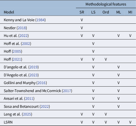

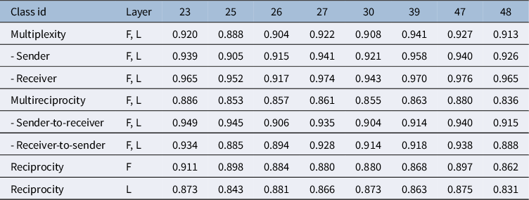
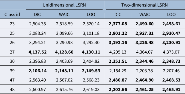
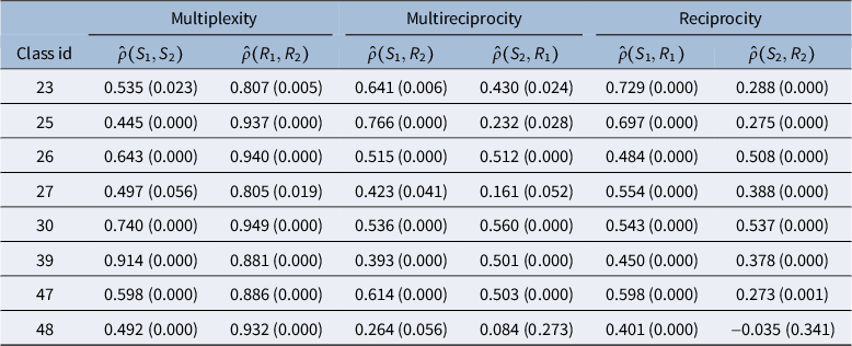

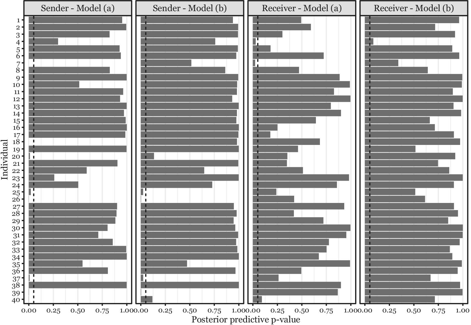
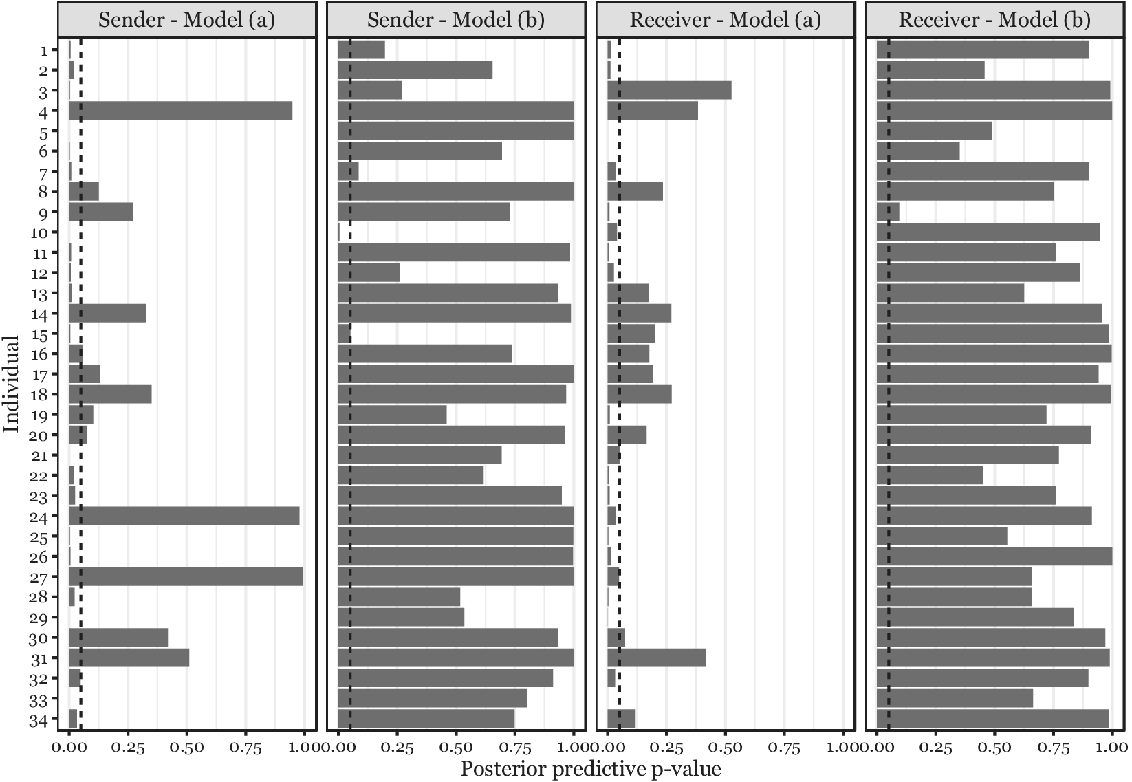
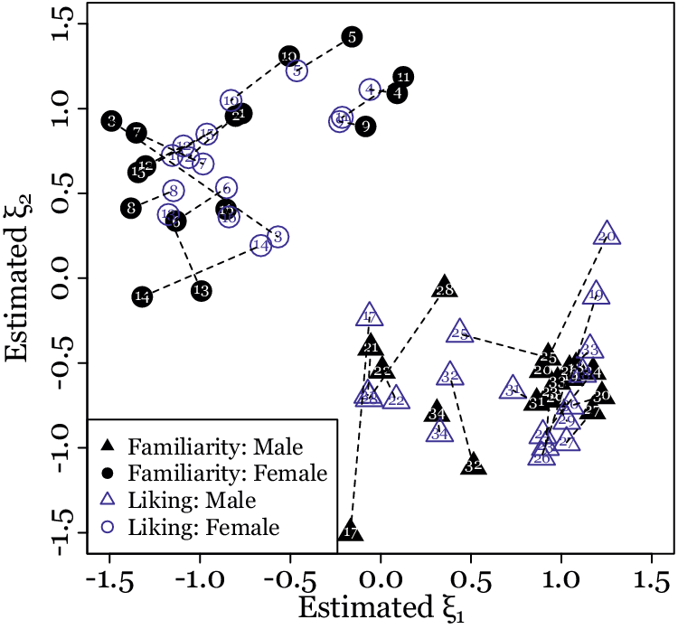

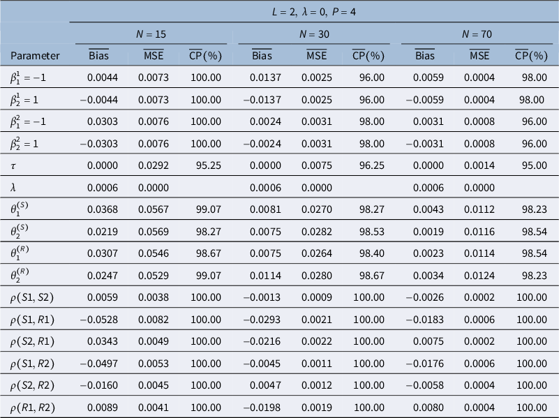


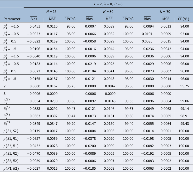


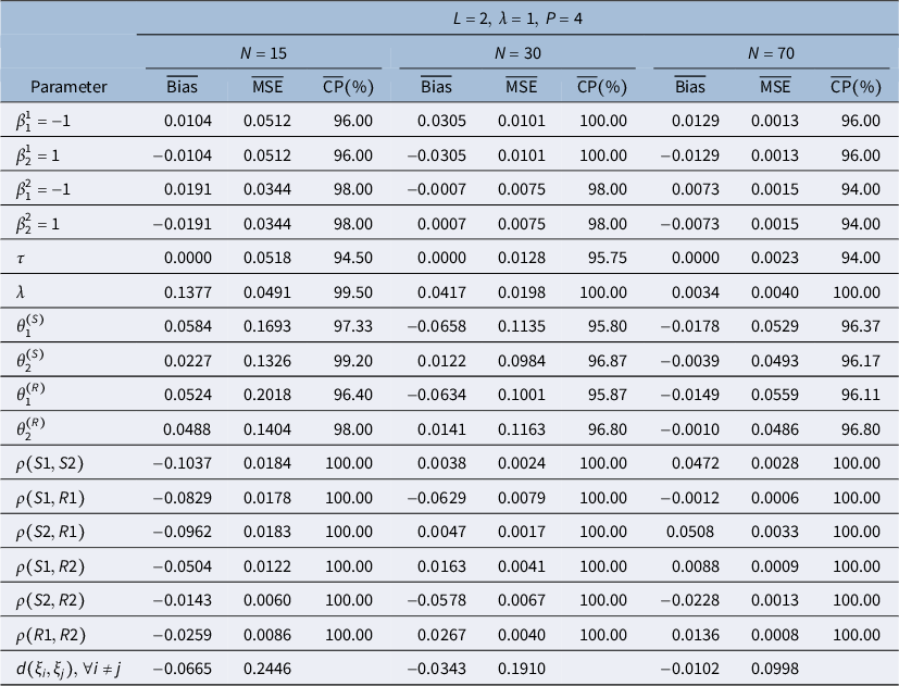


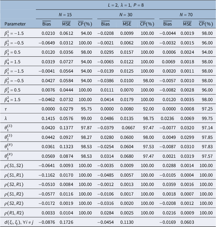


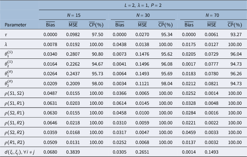


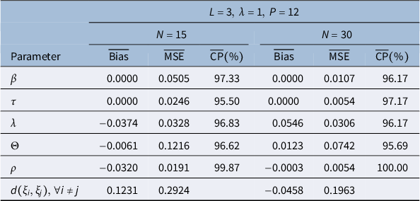


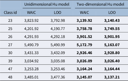
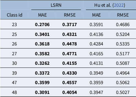
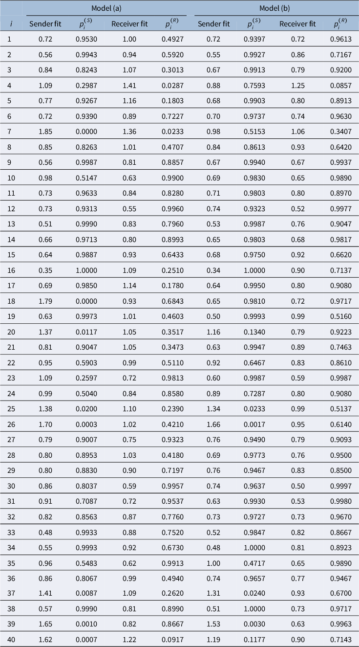
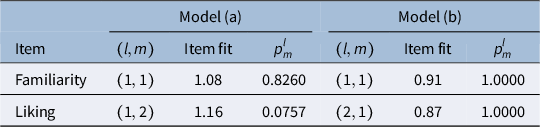
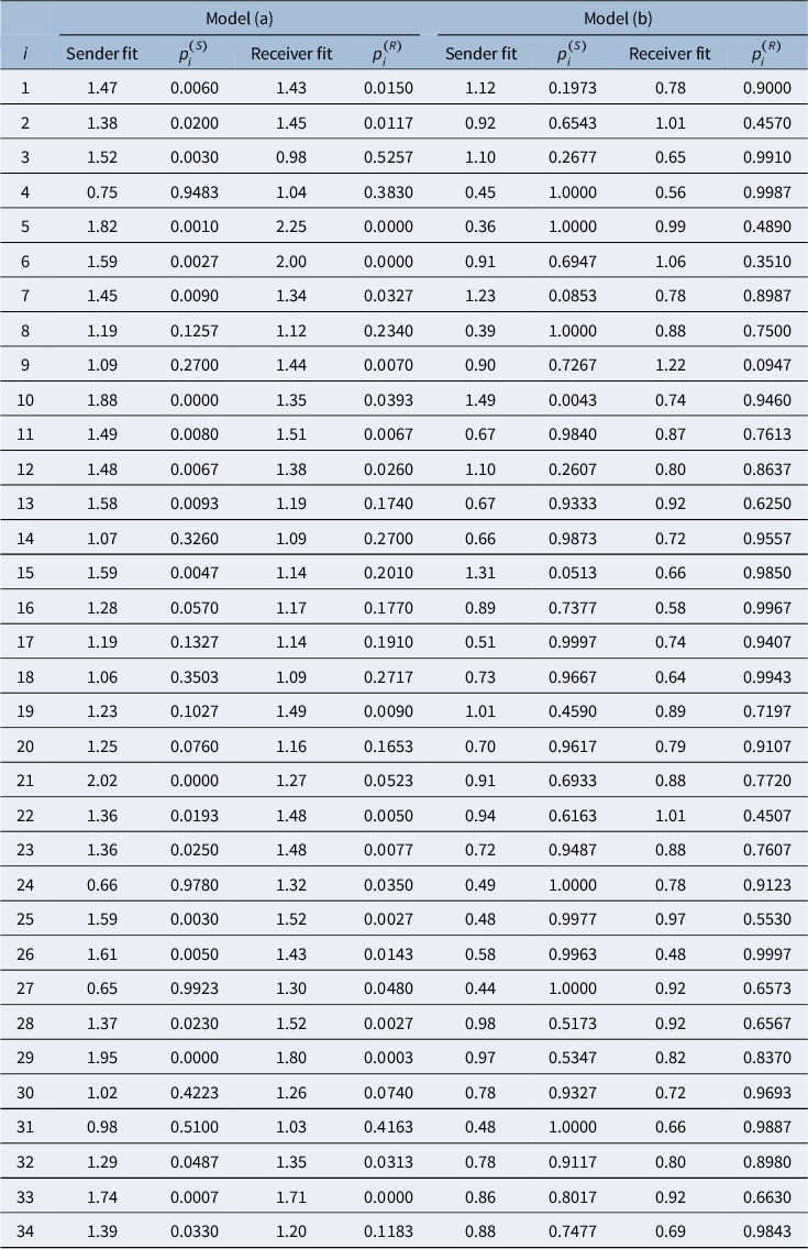
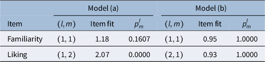
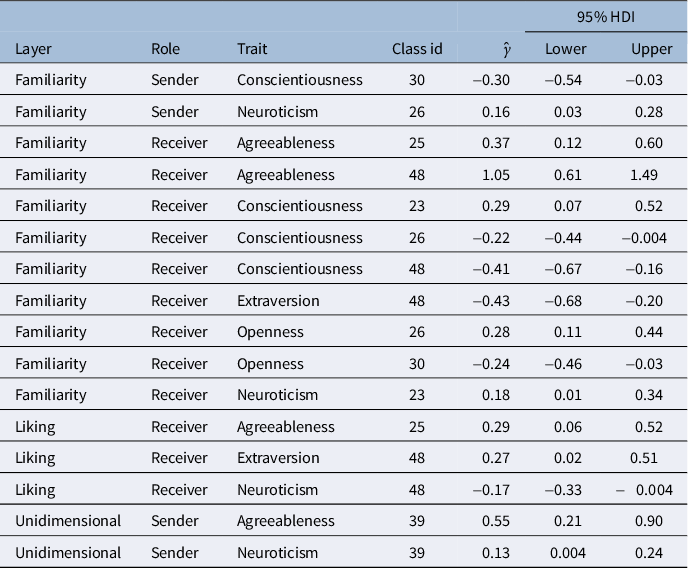
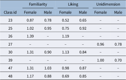
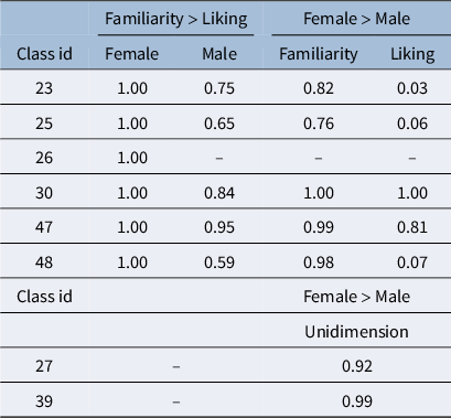
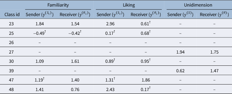

 Open access

