



1. Introduction
The dynamics of liquid film flows has fascinated scientists over many decades, which are central to numerous areas of engineering, geophysics and biophysics (Craster & Matar Reference Craster and Matar2009). As one of significant phenomena in liquid film flows, the bulge evolution on a film affected by gravity is common both in natural occurrences, like the ground ripples on a rainy day (Moss, Walker & Hutka Reference Moss, Walker and Hutka1979), and in engineering industries, such as bulges on a liquid film coating in the chemical industry (Shemilt et al. Reference Shemilt, Horsley, Jensen, Thompson and Whitfield2023) or a bulge excited by plasma currents on a liquid metal divertor (Allain, Ruzic & Hendricks Reference Allain, Ruzic and Hendricks2001). It is crucial to make clear the fluid mechanism of this entire process. Generally, the wavelength (denoted as
 $\lambda$
) of the wave generated by the evolution of the bulge under the action of gravity is much larger than the stationary film depth. Therefore, the physical model of such phenomena can be simplified as the bulge evolution on shallow water.
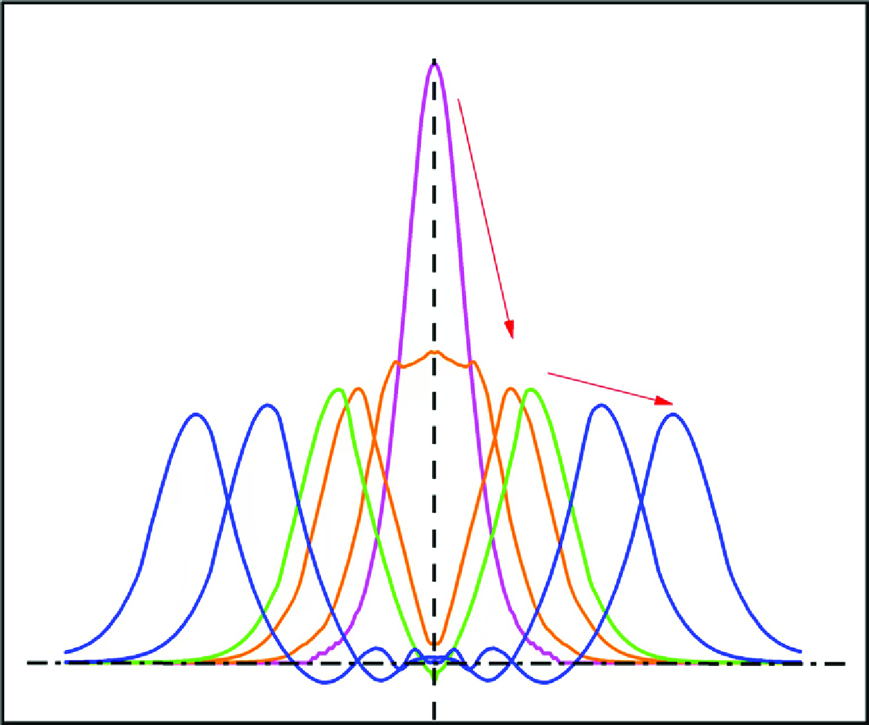
A diagrammatic sketch of the bulge on a film is presented in figure 1(a). Direct numerical simulation (DNS) is often employed to investigate the dynamics of wave evolution (Dhar, Das & Das Reference Dhar, Das and Das2020). The numerical procedures, numerical validations and case settings are given in the following section. With the help of DNS, a two-dimensional (2-D) axisymmetric bulge, whose initial profile is a solitary wave shape, evolves under the influence of gravity on a film. Its vertical section is shown in figure 1(b). The entire evolution indicates that there are probably two processes involved, which we outline here with the full details provided in the following sections. The first process is the collapse process, which occurs before the bulge height at the axisymmetric axis equalling the stationary film depth (the orange line in figure 1 b). In this stage, the bulge does not propagate as a wave directly, but instead diffuses out and forms a dominant crest around the axisymmetric axis. The dominant crest is referred to as the leading wave. The other process is the propagation process, which occurs after the formation of the leading wave (the blue line in figure 1 b). Subsequently, the leading wave begins to propagate along the radial direction connecting with a series of nonlinear wave trains.
Bulge evolution models. (a) A diagrammatic sketch of the bulge on a film. (b) The entire process of the bulge evolution obtained by DNS in a vertical section.

Although great efforts have been made to explore nonlinear long gravity waves, a comprehensive understanding of the entire process of bulge evolution in shallow water remains elusive. The collapse process of the bulge evolution resembles the spread of fluid drops over a horizontal plane by the influence of gravity. Nakaya (Reference Nakaya1974) studied the manner of flattening of the fluid drops and found that the free surface height satisfied the nonlinear diffusion equation by an asymptotic expansion. Hinton & Slim (Reference Hinton and Slim2023) investigated the dynamics of a viscous liquid spreading above a granular bed. The thickness of the viscous liquid, derived from their two-layer model, was controlled by a diffusion term. Furthermore, Kakutani & Matsuuchi (Reference Kakutani and Matsuuchi1975) derived an equation of the surface elevation for weakly nonlinear long gravity waves with low-Reynolds-number (Re) cases by a perturbation method. They found the effect of viscosity prevailing in the whole flow layer, whose wave evolution satisfied a nonlinear diffusion equation. This viscous dissipation dominant process cannot lead to wave propagation, which seems to occur in the present collapse process of bulge evolution.
As demonstrated in figure 1(b), the wave shape in the propagation process of bulge evolution exhibits one prominent wave crest towing a series of nonlinear wave trains. It is close to, but differs from, the solitary wave solution of the well-known Korteweg–de Vries (KdV) equation (Korteweg & De Vries Reference Korteweg and De Vries1895), which has only one wave crest. The KdV equation is established based on the balance between weak nonlinearity and weak dispersion. When the effects of geometrical distortion on a propagating gravity wave are comparable with those of amplitude nonlinearity and phase dispersion, its mathematical description can be reduced to some forms of a variable-coefficient KdV equation (Weidman & Zakhem Reference Weidman and Zakhem1988). The cylindrical KdV (C-KdV) equation (Johnson Reference Johnson1980), introduced for radially propagating waves, is such an example. The solitary wave solution of the C-KdV equation consists of three components: the leading deforming wave (a pulse), the trailing shelf compensating for the change of ‘mass’ in the leading wave and the nonlinear wave train (the oscillatory transition back to undisturbed conditions) (Grimshaw Reference Grimshaw2019). Miles (Reference Miles1977) has investigated the relationship between the wave height of the leading wave (denoted as
 $\eta$
) and the radial position (represented by
 $r$
), which found that the wave height of the leading wave followed a power law relationship, given by
 $\eta \sim {r^{ - 2/3}}$
. It is noted that the solitary wave solution of the C-KdV equation has a similar wave shape with the present propagation process of bulge evolution, but there are some different inherent mechanisms between them, which will be seen in § 3.2.5.
The physical mechanism underlying the collapse and propagation processes of bulge evolution, as well as their interactions, remain a subject of uncertainty. The present work aims to seek an analytical description of the detailed bulge evolution on shallow water and to explore the attenuation of wave height. Hence, two distinct processes (the diffusion process and the propagation process) of bulge evolution on shallow water will be theoretically modelled by using perturbation methods. Their derived scaling laws for wave height attenuation will be verified by DNS.
2. Governing equation and numerical method
2.1. Governing equations
Considering an incompressible Newtonian fluid subjected to an external gravity, the motion of bulge evolution is governed by two-phase flow equations in a dimensional form using the one-fluid model as
 \begin{align}& \frac {{\partial ( {\rho \boldsymbol{u}} )}}{{\partial t}} + \boldsymbol{\nabla } \boldsymbol{\cdot } ( {\rho \boldsymbol{u} \otimes \boldsymbol{u}} ) = - \nabla p + \nabla \boldsymbol{\cdot } \big[ {\mu \big( {\boldsymbol{\nabla } \boldsymbol{u} + (\boldsymbol{\nabla } \boldsymbol{u})^T} \big)} \big] + \rho \boldsymbol{g} + {\sigma }k_s\nabla c ,\end{align}
 \begin{align}&\qquad\qquad\qquad\qquad\qquad\qquad\qquad \boldsymbol{\nabla } \boldsymbol{\cdot } \boldsymbol{u} = 0, \end{align}
where the physical quantities
 $\boldsymbol{u}$
,
 $p$
,
 $t$
and
 $\boldsymbol{g}$
respectively represent the velocity, pressure, time and gravitational acceleration. The physical parameters
 $\rho$
,
 $\mu$
and
 $\sigma$
denote the fluid density, dynamic viscosity and surface tension coefficient, respectively. Based on the continuum surface tension (CSF) model (Brackbill, Kothe & Zemach Reference Brackbill, Kothe and Zemach1992), the surface tension can be expressed in the form of a volume force, where
 $k_s$
is the surface curvature and
 $c$
represents the volume fraction of the fluid.
2.2. Numerical method and validation
In the volume-of-fluid (VOF) method, the phase indicator function
 $\psi$
is characterised by a value of 1 in the fluid phase and 0 in the gas phase. In the absence of any phase transitions, the indicator function retains a constant value as each fluid element moves. As a result, the material derivative of
 $\psi$
is zero. The indicator function is updated in Eulerian form and is governed by the following advection equation:
 \begin{equation} \frac {{\partial \psi }}{{\partial t}} + \nabla \cdot ({\boldsymbol{u}}\psi ) = \psi \nabla \cdot {\boldsymbol{u}}. \end{equation}
Flow configuration of the cylindrical solitary wave and numerical method validation. (a) Flow configuration of the cylindrical solitary wave. (b) Comparision of the wave height’s scaling law of the solitary solution of the C-KdV equation with the theoretical result provided by Weidman & Zakhem (Reference Weidman and Zakhem1988). Numerical result (black dash dot line) and theoretical result (red line). The subscript
 $i$
denotes the selected initial value. All data points have been translated to start from an initial value of inlet position.

There are generally two categories of VOF methods: geometric approaches and algebraic approaches. In geometric methods, the phase indicator function
 $\psi$
is reconstructed using explicit geometric approximations, whereas algebraic methods describe
 $\psi$
through analytical expressions, such as polynomial or trigonometric functions (Mirjalili, Jain & Dodd Reference Mirjalili, Jain and Dodd2017). In the present numerical study, an algebraic VOF method, the tangent of hyperbola interface capturing (THINC) scheme with quadratic surface approximation and Gaussian quadrature (Xie & Xiao Reference Xie and Xiao2017), is employed to accurately resolve the dynamics of the free surface during the evolution of the bulge. This method assumes a hyperbolic tangent profile for the phase indicator function in cells where the interface exists. The Gaussian quadrature is then used to estimate the integration of the cell volume fraction and compute the phase fluxes from the reconstruction surface function. Detailed numerical procedures can be referred to in our previous work (Pan & Ni Reference Pan and Ni2022). A brief summary of the numerical procedures is given in Appendix A to facilitate understanding of the algorithm. To assess the accuracy of the numerical implementation for two-phase flow, the radial propagation of axisymmetric free-surface solitary waves, which is governed by the C-KdV equation (Miles Reference Miles1978), is examined. The following illustrates the flow configuration and grid arrangement. The flow configuration depicting the cylindrical wave is illustrated in figure 2(a). The computational domain encompasses a fan-shaped area spanning 30 degrees. The inlet boundary condition, as detailed in (2.4), includes the wave height profile and velocity profile, representing the solitary solution derived from Boussinesq theory (Lee, Skjelbreia & Raichlen Reference Lee, Skjelbreia and Raichlen1982). In this context, the variables
 $h$
,
 $H$
and
 $c_0$
represent the water depth, initial wave height and phase velocity. A symmetry condition is imposed on both sides, defined as Near Corner in the computational domain. The boundary conditions comprise a free outflow at the top of the domain, while a no-slip wall is enforced at the bottom. The outlet boundary conditions aim for an outgoing wave without reflection. A specific type of wave absorption method addressing dispersive effects (Wellens Reference Wellens2012) is employed, which performs well in linear and weakly nonlinear systems. Spanwise grid settings adopt an O-shaped grid.
 \begin{equation} \left \{ \begin{array}{l} \eta = H{{\mathrm{sech}} ^2}\left ( {\sqrt {\frac {{3H}}{{4{h^3}}}} (r - c_0t)} \right ),\\[12pt] u = \sqrt {gh} \frac {H}{h}{{\mathrm{sech}} ^2}\left ( {\sqrt {\frac {{3H}}{{4{h^3}}}} (r - c_0t)} \right ). \end{array} \right . \end{equation}
Heights of the leading wave obtained from the present numerical method are in good agreement with the scaling law derived from the theoretical study by Weidman & Zakhem (Reference Weidman and Zakhem1988), as depicted in figure 2(b). This comparison confirms the capability of numerical method to accurately simulate wave motion.
2.3. Flow configuration and grid independent test
Flow configuration and mesh arrangement. (a) Flow domain (original domain size:
 $20W\times 20W$
). Actual computational domain: a quarter of the original domain. (b) ‘Sandwich’ mesh arrangement.

The computational domain for bulge evolution is illustrated in figure 3(a). The domain’s length and width are both defined as
 $20W$
, where
 $W$
denotes the width of initial bulge. According to Boussinesq solitary wave theory, the wavelength corresponding to 99.26 % of the solitary wave height is chosen as the initial bulge width
 $W = 4\pi \sqrt {h^3/3H}$
. For some other initial bulge,
 $W$
is defined as half of the wavelength for a cosine shape or the diameter for a cylindrical shape. The height of the domain is determined by
 $h+1.1H$
, where
 $h$
and
 $H$
represent the initial stationary liquid depth and the initial bulge height, respectively. The bulge is situated at the centre of the domain. Based on the axisymmetry of the fluid dynamics for bulge evolution, the computational domain is reduced to a quarter of the original size to optimise computational efficiency. Hence, a quarter of the bulge originates from a corner, which is the centre of the original domain. A symmetry condition is imposed on both sides near this corner within the new domain. The boundary conditions at the top, bottom and outlet are consistent with the cylindrical solitary wave case.
To accurately capture the interface while saving computation time, the grid arrangement is designed akin to a ‘sandwich’, as demonstrated in figure 3(b). In the vertical direction, the grid is denser and uniform near the wave surface to provide higher resolution for capturing free surface details accurately. In the middle of the fluid depth, the grid becomes progressively sparser, while it gradually increases in density towards the bottom wall to capture the boundary layer. In the horizontal direction, a uniform grid is set. Table 1 gives the testing of three different meshes, characterised by various parameters. Here,
 $\Delta {z_{uni}}$
signifies the uniform vertical grid size near the wave surface, while
 $\Delta {z_{\textit{min}}}$
and
 $\Delta {z_{\textit{max}}}$
respectively denote the finest and the sparest grid sizes within the non-uniform grid. Moreover,
 $\varDelta _{//}$
refers to the uniform horizontal grid resolution. The physical properties of GaInSn for the liquid phase and air for the gas phase are selected (Yang et al. Reference Yang, Qi, Ni and Wang2016). The liquid properties are the density
 ${\rho _l} = 6360\,\rm kg\,{m^{ - 3}}$
and the kinematic viscosity
 ${\upsilon _l} = 2.98 \times {10^{ - 7}}\,\rm {m^2}\,{s^{ - 1}}$
, while their corrresponding gas properties are
 ${\rho _g} = 1.225\,\rm kg\,{m^{ - 3}}$
and
 ${\upsilon _g} = 1.46 \times {10^{ - 5}}\,\rm {m^2}\,{s^{ - 1}}$
. The surface tension between liquid and gas is denoted by
 $\sigma = 0.533\,\rm kg\,{s^{ - 2}}$
. Figure 4(a) illustrates the comparison of wave shapes among these three different meshes, which indicates that the mesh2 can effectively capture the wave evolution and simultaneously save computational costs. Therefore, the mesh2 (about 35 million grid numbers) is adopted for subsequent simulations. Furthermore, figure 4(b) shows that the wave height evolution curves obtained from simulations using the quarter domain and the full domain coincide well, which confirms the reasonability of using the quarter domain.
The grid independence test. Uniform vertical grid size
 $\Delta {z_{uni}}$
near the wave surface. The finest grid size
 $\Delta {z_{\textit{min}}}$
and the sparest grid size
 $\Delta {z_{\textit{max}}}$
in the remaining non-uniform grid. The horizontal grid size
 $\varDelta _{//}$
.

Grid independent test for an initial bulge profile approximating a solitary wave. (a) Comparison of the results for different types of meshes (
 $h=0.12, H=0.002$
). (b) The comparison of wave height evolution between the quarter domain and the full original domain (
 $h=0.1, H=0.1$
).

3. Theoretical analysis
The focus of this article is on the evolution of an initially axisymmetric bulge under the influence of gravity on shallow water. We aim to develop a possible theoretical framework for describing bulge evolution under weakly nonlinear long gravity wave assumptions. Under the condition of shallow water, it is generally expected that the surface tension may be considered negligible in the present long-wave approximation. Dimensionless flow variables, such as the length (radial
 $r$
and normal
 $z$
), time (
 $t$
), velocity (radial
 $u$
and normal
 $w$
) and pressure (
 $p$
) are scaled with
 $h$
,
 $h/c_0$
,
 $c_0$
and
 $\rho gh$
, respectively. Here,
 $c_0 = \sqrt {gh}$
is the linear phase speed of infinitely long waves. Then, non-dimensional two-dimensional axisymmetric flow equations are governed by
 \begin{align} \left \{ \begin{array}{l} \displaystyle {\frac {1}{{\tilde r}}\frac {\partial }{{\partial \tilde r}}\left ( {\tilde r\tilde u} \right ) + \frac {{\partial \tilde w}}{{\partial \tilde z}} = 0},\\[10pt] \displaystyle {\frac {{\partial \tilde u}}{{\partial \tilde t}} + \tilde u\frac {{\partial \tilde u}}{{\partial \tilde r}} + \tilde w\frac {{\partial \tilde u}}{{\partial \tilde z}} = - \frac {{\partial \tilde p}}{{\partial \tilde r}} + \frac {1}{{{{Re}}}}\left ( {\frac {{{\partial ^2}\tilde u}}{{\partial {{\tilde z}^2}}} + \frac {1}{{\tilde r}}\frac {\partial }{{\partial \tilde r}}\left ( {\tilde r\frac {{\partial \tilde u}}{{\partial \tilde r}}} \right ) - \frac {{\tilde u}}{{{{\tilde r}^2}}}} \right )},\\[13pt] \displaystyle {\frac {{\partial \tilde w}}{{\partial \tilde t}} + \tilde u\frac {{\partial \tilde w}}{{\partial \tilde r}} + \tilde w\frac {{\partial \tilde w}}{{\partial \tilde z}} = - \frac {{\partial \tilde p}}{{\partial \tilde z}} - 1 + \frac {1}{{{{Re}}}}\left ( {\frac {{{\partial ^2}\tilde w}}{{\partial {{\tilde z}^2}}} + \frac {1}{{\tilde r}}\frac {\partial }{{\partial \tilde r}}\left ( {\tilde r\frac {{\partial \tilde u}}{{\partial \tilde r}}} \right )} \right )}, \end{array} \right . \end{align}
 \begin{align} \left \{ \begin{array}{l} \displaystyle {\tilde u = \tilde w = 0\quad at\quad \tilde z = - 1;\quad \tilde w = \frac {{\partial \tilde \eta }}{{\partial \tilde t}} + \tilde u\frac {{\partial \tilde \eta }}{{\partial \tilde r}}\quad at\quad \tilde z = \tilde \eta \left ( {\tilde r,\tilde t} \right )},\\[10pt] \displaystyle {\left ( {\frac {{\partial \tilde u}}{{\partial \tilde z}} + \frac {{\partial \tilde w}}{{\partial \tilde r}}} \right )\left [ {1 - {{\left ( {\frac {{\partial \tilde \eta }}{{\partial \tilde r}}} \right )}^2}} \right ] + 2\left ( {\frac {{\partial \tilde w}}{{\partial \tilde z}} - \frac {{\partial \tilde u}}{{\partial \tilde r}}} \right )\frac {{\partial \tilde \eta }}{{\partial \tilde r}} = 0\quad at\quad \tilde z = \tilde \eta \left ( {\tilde r,\tilde t} \right )},\\[15pt] \displaystyle {\left ( {{{\tilde p}_\infty } - \tilde p} \right )\left [ {1 + {{\left ( {\frac {{\partial \tilde \eta }}{{\partial \tilde r}}} \right )}^2}} \right ] + \frac {2}{{{{Re}}}}\left [ {\frac {{\partial \tilde w}}{{\partial \tilde z}} + \frac {{\partial \tilde u}}{{\partial \tilde r}}{{\left ( {\frac {{\partial \tilde \eta }}{{\partial \tilde r}}} \right )}^2} - \frac {{\partial \tilde u}}{{\partial \tilde z}}\frac {{\partial \tilde \eta }}{{\partial \tilde r}} - \frac {{\partial \tilde w}}{{\partial \tilde r}}\frac {{\partial \tilde \eta }}{{\partial \tilde r}}} \right ] = 0}.\\[15pt] \displaystyle { \quad at\quad \tilde z = \tilde \eta \left ( {\tilde r,\tilde t} \right )} \end{array} \right . \end{align}
The free surface is described by the equation
 $\tilde z = \tilde \eta (\tilde r,\tilde t)$
. The surface of the stationary film is located at
 $z = 0$
with a horizontal bottom situated at
 $z = -h$
. In terms of boundary conditions, the no-slip condition is applied at the bottom of the film, while the kinematical and dynamical conditions (Kalliadasis et al. Reference Kalliadasis, Ruyer-Quil, Scheid and Velarde2012; Lunz & Howell Reference Lunz and Howell2019) are applied to the free surface. Here,
 ${{\tilde p}_\infty }$
is the dimensionless atmospheric pressure and the Reynolds number is defined as
 ${{Re}} = {c_0}h/\upsilon _l$
.
In § 1, the numerical results for a particular initial solitary profile are shown in figure 1(b). Initially, the solitary wave-like bulge exhibits a concentrated peak at the centre (depicted in pink). Over time, the peak of the initial bulge diminishes in amplitude (along the
 $z$
-axis) because of gravity, while the bulge collapses and propagates radially (
 $r$
-direction), giving rise to subsequent wavefronts (indicated in orange, green and blue). At a certain point in time, the wave height along the axis decreases to the stationary water level, indicating the formation of a well-defined propagating wave structure (depicted in green). Subsequently, as time continues to progress, the generated wavefront, which is generally called a leading wave, continues to propagate outward while gradually decreasing in height (depicted in blue). During the process from the collapse of the initial bulge to the formation of a well-defined propagating wave structure, the viscosity within the fluid plays a dominant role, resulting in a relatively low Re, which is referred to as the collapse process. Following this, the subsequent process where the newly formed leading wave propagates outward is characterised by a high Re and is referred to as the propagation process.
3.1. Collapse process
3.1.1. Decomposition of collapse sub-processes
An initial profile of bulge is depicted by an orange line in figure 5(a). As time proceeds, the whole of the initial bulge is collapsing and spreading outwards due to gravity, with the collapse occurring from its axisymmetric centre towards the surrounding stationary film. Hence, this process is named the ‘collapse process’. During the collapse process, it is generally expected that the hydrostatic pressure at the centre of the bulge is greater than that of the surrounding zone. Under the influence of gravity, the bulge collapses and ‘squeezes’ outward. Obviously, after a certain period, as depicted in figure 5(a), the centre bulge height, which corresponds to the peak of the initial bulge (orange line), descends below the surrounding zone, forming what can be referred to as a ‘basin’ (green line). This phenomenon indicates that fluids move from the centre to the surrounding zone, resulting in a new wavefront around it. To facilitate analyses and discussions, we designate the shape where the bulge’s centre height is slightly below the height of the surrounding zone as the ‘transition shape’. It is noticeable that the process from the start of collapse to the formation of the ‘transition shape’ is influenced by the surrounding flow fluid and gradually squeezes a new wavefront.
Collapse process. (a) Sub-process I: squeezing process. (b) Sub-process II: diffusion process.

Once the centre height of the bulge falls below the surrounding zone, from the perspective of energy, the gravitational potential energy at the centre of the bulge is converted into the kinetic energy of the newly extruded wavefront. This wavefront, acting as a leading wave, propagates radially outwards. It is generally considered that the new wavefront corresponds to propagation with a high Re, while the diffusion behaviour of the centre has a low Re of the order of
 $O(1)$
(Kakutani & Matsuuchi Reference Kakutani and Matsuuchi1975). Therefore, the newly formed wavefront will continue to move with a significantly higher overall velocity, as shown in figure 5(b). At the stage from the formation of ‘transition shape’ to the point where the centre height of the bulge reaches the stationary water level, the centre of the bulge diffuses out without being influenced by the surrounding propagating leading wave. For further analysis, we will divide the collapse process into two distinct sub-processes. Sub-process I begins with the initial shape of the bulge and ends with the ‘transition shape’, during which the decrease in central wave height is significantly influenced by the surrounding fluid and squeezes out new wavefronts. Therefore, this is referred to as the ‘squeezing process’. While sub-process II commences with the ‘transition shape’ and extends until the end of the collapse process, where the centre of the bulge diffuses without influence from the surrounding new wavefronts, thus constituting a ‘diffusion process’.
To rigorously justify that the propagating leading wave will move with a significantly higher overall velocity and will not affect the diffusion process, we monitor the overall velocities of these two processes as shown in figure 6. In the diffusion process at time instance
 $t_1$
in figure 6(a), we use the wave height
 $H'$
at the symmetrical axis to reconstruct a corresponding solitary wave with the identical height. Then, we find the measurement point on the solitary wave with a half-wave height. We use the radius velocity component of the measurement point to represent the overall velocity of the diffusion process
 $U_d$
. As for the propagation process in figure 6(b), its overall velocity can be easily evaluated by the phase velocity
 $U_p = ({r_3-r_2})/({t_3-t_2})$
. Our DNS results indicate that the overall velocities of these two processes have a relationship
 $U_d/U_p\sim O(10^{-2})$
, which prove that the diffusion process is an independent process.
Overall velocity measurements. (a) Diffusion process. (b) Propagation process.

3.1.2. Scaling and perturbation analyses
Due to the interaction of the surrounding fluid, the squeezing process is a relatively complex phenomenon, making it difficult to characterise the wave height variation using a simple equation. In contrast, the diffusion at the centre of the bulge is not significantly influenced by the surrounding new wavefront during the diffusion process. Therefore, we will conduct a detailed modelling analysis specifically for the diffusion process. In the diffusion process, our main objective is to derive a simplified equation for the surface elevation under the assumption of weak nonlinearity and long wavelength. Similar to the approach used by Kakutani & Matsuuchi (Reference Kakutani and Matsuuchi1975) for studying a 2-D diffusion problem, the slow radial variable and slow time variable are adopted:
 $\tilde \xi = \varepsilon \tilde r;\tilde \tau = {\varepsilon ^2}\tilde t$
, which are substituted into (3.1) and (3.2). These transformations are required to ensure that
 $\alpha$
is of order
 $\varepsilon$
. Here,
 $\varepsilon = \eta /h$
represents the amplitude parameter, measuring nonlinearity, and
 $\alpha = h/\lambda$
represents the long-wave parameter, measuring dispersion. The undisturbed steady state without the bulge collapse is
 $\tilde u = \tilde w = 0$
and
 $\tilde p = {\tilde p_\infty } - \tilde z$
. By introducing (3.3), the form of asymptotic multiple-scale expansions, into the governing equations and combining with boundary conditions, a sequence of equations and boundary conditions for each order of
 $\varepsilon$
can be obtained. It is noted that any field quantity
 $\tilde \phi (\tilde \xi ,\tilde z = \tilde \eta ,\tilde \tau )$
at the free surface boundary condition can be expressed as a Taylor expansion equation (3.4) at the position
 $\tilde z_0$
to match the multiple-scale expansions in the governing equations.
 \begin{align}& \left \{ \begin{array}{l} \tilde u\big( {\tilde \xi ,\tilde z,\tilde \tau } \big) = \sum \limits _{n = 0}^\infty {{\varepsilon ^n}{{\tilde u}_n}\big( {\tilde \xi ,\tilde z,\tilde \tau } \big)} ;\quad \tilde w\big( {\tilde \xi ,\tilde z,\tilde \tau } \big) = \sum \limits _{n = 0}^\infty {{\varepsilon ^n}{{\tilde w}_n}\big( {\tilde \xi ,\tilde z,\tilde \tau } \big)}, \\ \tilde p\big( {\tilde \xi ,\tilde z,\tilde \tau } \big) = {{\tilde p}_\infty } - \tilde z + \sum \limits _{n = 0}^\infty {{\varepsilon ^n}{{\tilde p}_n}\big( {\tilde \xi ,\tilde z,\tilde \tau } \big)} ;\quad \tilde \eta \big( {\tilde \xi ,\tilde \tau } \big) = \sum \limits _{n = 0}^\infty {{\varepsilon ^n}{{\tilde \eta }_n}\big( {\tilde \xi ,\tilde \tau } \big)}, \end{array} \right . \end{align}
 \begin{align}&\qquad\qquad \tilde \phi \big( {\tilde \xi ,\tilde z = \tilde \eta ,\tilde \tau } \big) = { {\tilde \phi } \Bigg|_{\tilde z = {{\tilde z }_0}}} + {\left . {\frac {{\partial \tilde \phi }}{{\partial \tilde z}}} \right |_{\tilde z = {{\tilde z }_0}}}\left ( {\sum \limits _{n = 1}^\infty {{\varepsilon ^n}{{\tilde \eta }_n}\big( {\tilde \xi ,\tilde \tau } \big)} } \right ) + \ldots \\[12pt] \nonumber \end{align}
Due to the prevailing effect of viscous dissipation, the weaker nonlinearity cannot balance the dominant viscous dissipation, the position of Taylor expansion is selected as
 $\tilde z_0 = {\tilde \eta }_0$
for diffusion process in this section and
 $\tilde z_0 = 0$
for propagation process in next section (Kakutani & Matsuuchi Reference Kakutani and Matsuuchi1975). After substituting these expressions (3.3) and (3.4), the governing equation takes the form:
 \begin{equation} \left \{ \begin{array}{l} \displaystyle {\frac {{\partial {{\tilde w}_0}}}{{\partial \tilde z}} + \varepsilon \left(\frac {{{{\tilde u}_0}}}{{\tilde \xi }} + \frac {{\partial {{\tilde u}_0}}}{{\partial \tilde \xi }} + \frac {{\partial {{\tilde w}_1}}}{{\partial \tilde z}}\right) + {\varepsilon ^2}\left(\frac {{{{\tilde u}_1}}}{{\tilde \xi }} + \frac {{\partial {{\tilde u}_1}}}{{\partial \tilde \xi }} + \frac {{\partial {{\tilde w}_2}}}{{\partial \tilde z}}\right) = 0} \\[13pt] \displaystyle {{{\tilde w}_0}\frac {{\partial {{\tilde u}_0}}}{{\partial \tilde z}} - \frac {1}{{{{Re}} }}\frac {{{\partial ^2}{{\tilde u}_0}}}{{\partial {{\tilde z}^2}}} + \varepsilon \left({{\tilde u}_0}\frac {{\partial {{\tilde u}_0}}}{{\partial \tilde \xi }} + {{\tilde w}_0}\frac {{\partial {{\tilde u}_1}}}{{\partial \tilde z}} + {{\tilde w}_1}\frac {{\partial {{\tilde u}_0}}}{{\partial \tilde z}} + \frac {{\partial {{\tilde p}_0}}}{{\partial \tilde \xi }} - \frac {1}{{{{Re}} }}\frac {{{\partial ^2}{{\tilde u}_1}}}{{\partial {{\tilde z}^2}}}\right)} \\[13pt] \displaystyle { + {\varepsilon ^2}\left(\frac {{\partial {{\tilde u}_0}}}{{\partial \tilde \tau }} + {{\tilde u}_0}\frac {{\partial {{\tilde u}_1}}}{{\partial \tilde \xi }} + {{\tilde u}_1}\frac {{\partial {{\tilde u}_0}}}{{\partial \tilde \xi }} + {{\tilde w}_0}\frac {{\partial {{\tilde u}_2}}}{{\partial \tilde z}} + {{\tilde w}_1}\frac {{\partial {{\tilde u}_1}}}{{\partial \tilde z}} + {{\tilde w}_2}\frac {{\partial {{\tilde u}_0}}}{{\partial \tilde z}} + \frac {{\partial {{\tilde p}_1}}}{{\partial \tilde \xi }}\right .} \\[13pt] \displaystyle { \left . - \frac {1}{{{{Re}} }}\frac {{{\partial ^2}{{\tilde u}_2}}}{{\partial {{\tilde z}^2}}} + \frac {1}{{{{Re}} }}\frac {{{{\tilde u}_0}}}{{{{\tilde \xi }^2}}} - \frac {1}{{{{Re}} }}\frac {1}{{\tilde \xi }}\frac {{\partial {{\tilde u}_0}}}{{\partial \tilde \xi }} + \frac {1}{{{{Re}} }}\frac {{{\partial ^2}{{\tilde u}_0}}}{{\partial {{\tilde \xi }^2}}}\right) = 0} \\[13pt] \displaystyle {{{\tilde w}_0}\frac {{\partial {{\tilde w}_0}}}{{\partial \tilde z}} + \frac {{\partial {{\tilde p}_0}}}{{\partial \tilde z}} - \frac {1}{{{{Re}} }}\frac {{{\partial ^2}{{\tilde w}_0}}}{{\partial {{\tilde z}^2}}} + \varepsilon \left({{\tilde u}_0}\frac {{\partial {{\tilde w}_0}}}{{\partial \tilde \xi }} + {{\tilde w}_1}\frac {{\partial {{\tilde w}_0}}}{{\partial \tilde z}} + {{\tilde w}_0}\frac {{\partial {{\tilde w}_1}}}{{\partial \tilde z}} + \frac {{\partial {{\tilde p}_1}}}{{\partial \tilde z}} - \frac {1}{{{{Re}} }}\frac {{{\partial ^2}{{\tilde w}_1}}}{{\partial {{\tilde z}^2}}}\right)} \\[13pt] \displaystyle {+ {\varepsilon ^2}\left(\frac {{\partial {{\tilde w}_0}}}{{\partial \tilde \tau }} + {{\tilde u}_1}\frac {{\partial {{\tilde w}_0}}}{{\partial \tilde \xi }} + {{\tilde u}_0}\frac {{\partial {{\tilde w}_1}}}{{\partial \tilde \xi }} + {{\tilde w}_1}\frac {{\partial {{\tilde w}_1}}}{{\partial \tilde z}} + {{\tilde w}_0}\frac {{\partial {{\tilde w}_2}}}{{\partial \tilde z}} + {{\tilde w}_2}\frac {{\partial {{\tilde w}_0}}}{{\partial \tilde z}}\right .}\\[13pt] \displaystyle {\left . + \frac {{\partial {{\tilde p}_2}}}{{\partial \tilde z}} - \frac {1}{{{{Re}} }}\frac {{{\partial ^2}{{\tilde w}_2}}}{{\partial {{\tilde z}^2}}} - \frac {1}{{{{Re}} }}\frac {1}{{\tilde \xi }}\frac {{\partial {{\tilde w}_0}}}{{\partial \tilde \xi }} - \frac {1}{{{{Re}} }}\frac {{{\partial ^2}{{\tilde w}_0}}}{{\partial {{\tilde \xi }^2}}}\right) = 0}. \end{array} \right . \end{equation}
Correspondingly, the boundary condition becomes
 \begin{equation} \left \{ \begin{array}{l} \displaystyle {\tilde u = \tilde w = 0\quad at\quad \tilde z = 0} \\[5pt] \displaystyle {{{\tilde w}_0} + {\varepsilon ^1}\left({{\tilde \eta }_1}\frac {{\partial {{\tilde w}_0}}}{{\partial \tilde z}} + {{\tilde w}_1} - {{\tilde u}_0}\frac {{\partial {{\tilde \eta }_0}}}{{\partial \tilde \xi }}\right) + {\varepsilon ^2}\left[{{\tilde \eta }_2}\frac {{\partial {{\tilde w}_0}}}{{\partial \tilde z}} + {{\tilde \eta }_1}\frac {{\partial {{\tilde w}_1}}}{{\partial \tilde z}} + {{\tilde w}_2}\right .} \\[10pt] \displaystyle {\left .-\, \frac {{\partial {{\tilde \eta }_0}}}{{\partial \tilde \tau }} - {{\tilde u}_0}\frac {{\partial {{\tilde \eta }_1}}}{{\partial \tilde \xi }} - \left({{\tilde \eta }_1}\frac {{\partial {{\tilde u}_0}}}{{\partial \tilde z}} + {{\tilde u}_1}\right)\frac {{\partial {{\tilde \eta }_0}}}{{\partial \tilde \xi }}\right] = 0\quad at\quad \tilde z = 1 + {{\tilde \eta }_0}} \\[10pt] \displaystyle \frac {{\partial {{\tilde u}_0}}}{{\partial \tilde z}} + {{\varepsilon}^1} \left[\frac {{\partial \left({{\tilde \eta }_1}\frac {{\partial {{\tilde u}_0}}}{{\partial \tilde z}} + {{\tilde u}_1}\right)}}{{\partial \tilde z}} + \frac {{\partial {{\tilde w}_0}}}{{\partial \tilde \xi }}+ 2\frac {{\partial {{\tilde w}_0}}}{{\partial \tilde z}}\frac {{\partial {{\tilde \eta }_0}}}{{\partial \tilde \xi }}\right] \\[10pt] \displaystyle { +\, {\varepsilon ^2}\left\{ \frac {{\partial \left({{\tilde \eta }_2}\frac {{\partial {{\tilde u}_0}}}{{\partial \tilde z}} + {{\tilde \eta }_1}\frac {{\partial {{\tilde u}_1}}}{{\partial \tilde z}} + {{\tilde u}_2}\right)}}{{\partial \tilde z}} + \frac {{\partial \left({{\tilde \eta }_1}\frac {{\partial {{\tilde w}_0}}}{{\partial \tilde z}} + {{\tilde w}_1}\right)}}{{\partial \tilde \xi }} - \frac {{\partial {{\tilde u}_0}}}{{\partial \tilde z}}{\left(\frac {{\partial {{\tilde \eta }_0}}}{{\partial \tilde \xi }}\right)^2}\right .} \\[15pt] \displaystyle {\left . +\, 2 \left[\frac {{\partial \left({{\tilde \eta }_1}\frac {{\partial {{\tilde w}_0}}}{{\partial \tilde z}} + {{\tilde w}_1}\right)}}{{\partial \tilde z}} - \frac {{\partial {{\tilde u}_0}}}{{\partial \tilde \xi }}\right]\frac {{\partial {{\tilde \eta }_0}}}{{\partial \tilde \xi }} + 2\frac {{\partial {{\tilde w}_0}}}{{\partial \tilde z}}\frac {{\partial {{\tilde \eta }_1}}}{{\partial \tilde \xi }}\right\} = 0\quad at\quad \tilde z = 1 + {{\tilde \eta }_0}} \\[15pt] \displaystyle { -\, {{\tilde p}_0} + {{\tilde \eta }_0} + \frac {2}{{{{Re}} }}\frac {{\partial {{\tilde w}_0}}}{{\partial \tilde z}} + {\varepsilon ^1}\left[\frac {2}{{{{Re}} }}\frac {{\partial \left({{\tilde \eta }_1}\frac {{\partial {{\tilde w}_0}}}{{\partial \tilde z}} + {{\tilde w}_1}\right)}}{{\partial \tilde z}} - \left({{\tilde \eta }_1}\frac {{\partial {{\tilde p}_0}}}{{\partial \tilde z}} + {{\tilde p}_1} - {{\tilde \eta }_1}\right)\right .} \\[20pt] \displaystyle {\left . -\, \frac {2}{{{{Re}} }}\frac {{\partial {{\tilde u}_0}}}{{\partial \tilde z}}\frac {{\partial {{\tilde \eta }_0}}}{{\partial \tilde \xi }}\right] + {\varepsilon ^2}\left\{ {\left(\frac {{\partial {{\tilde \eta }_0}}}{{\partial \tilde \xi }}\right)^2}\left ( { - {{\tilde p}_0} + {{\tilde \eta }_0}} \right ) - \left({{\tilde \eta }_2}\frac {{\partial {{\tilde p}_0}}}{{\partial \tilde z}} + {{\tilde \eta }_1}\frac {{\partial {{\tilde p}_1}}}{{\partial \tilde z}} + {{\tilde p}_2} - {{\tilde \eta }_2}\right) \right .} \\[13pt] \displaystyle {\left .+\, \frac {2}{{{{Re}} }}\frac {{\partial \left({{\tilde \eta }_2}\frac {{\partial {{\tilde w}_0}}}{{\partial \tilde z}} + {{\tilde \eta }_1}\frac {{\partial {{\tilde w}_1}}}{{\partial \tilde z}} + {{\tilde w}_2}\right)}}{{\partial \tilde z}} \right .} \\[13pt] \displaystyle {\left .-\, \frac {2}{{{{Re}} }}\left[\frac {{\partial \left({{\tilde \eta }_1}\frac {{\partial {{\tilde u}_0}}}{{\partial \tilde z}} + {{\tilde u}_1}\right)}}{{\partial \tilde z}}\frac {{\partial {{\tilde \eta }_0}}}{{\partial \tilde \xi }} + \frac {{\partial {{\tilde u}_0}}}{{\partial \tilde z}}\frac {{\partial {{\tilde \eta }_1}}}{{\partial \tilde \xi }} + \frac {{\partial {{\tilde w}_0}}}{{\partial \tilde \xi }}\frac {{\partial {{\tilde \eta }_0}}}{{\partial \tilde \xi }}\right]\right\} = 0\quad at\quad \tilde z = 1 + {{\tilde \eta }_0}}. \end{array} \right . \end{equation}
With these multiple-scale expansion equations, the leading order solution of
 $\tilde \eta$
satisfying the following nonlinear diffusion equation is given as
 \begin{equation} \frac {{\partial {{\tilde \eta }_0}}}{{\partial \tilde \tau }} = \frac {{{{Re}} }}{{3\tilde \xi }}\frac {\partial }{{\partial \tilde \xi }}\left [ {{{\left ( {1 + {{\tilde \eta }_0}} \right )}^3}\tilde \xi \frac {{\partial {{\tilde \eta }_0}}}{{\partial \tilde \xi }}} \right ] .\end{equation}
This equation is consistent with the diffusion equation derived by Nakaya (Reference Nakaya1974) in his study of the spread of a viscous droplet under gravity on a plane, which indicates that both belong to the same diffusion process. Furthermore, it also proves that during the diffusion process the surrounding leading wave exerts negligible influence on the centre of the bulge.
Validations for diffusion process. (a) The DNS evolution of the wave height during the whole collapse process. All data points have been translated to start from an initial value of zero. The subscript
 $i$
denotes the selected initial value. Here,
 $h=0.3$
and
 $H=0.03$
are given with an initial bulge profile approximating a solitary wave. (b) Verification of scaling laws between wave height and time of diffusion process. All data points have been translated to start from an initial value of zero. The subscript
 $i$
denotes the selected initial value. The numbers following
 $h$
,
 $H$
,
 $W$
represent their values, expressed in SI units. The black solid lines, each with a slope of 45 degrees, indicate the trend given by the theoretically derived scaling law.

3.1.3. Normalisation of the scaling law
According to Landau & Lifshitz (Reference Landau and Lifshitz1987), (3.7) is solved by introducing the volume flow of bulge,
 $\tilde {q}$
, and the scaling law for the wave height at the central axis of the bulge over time is obtained:
 \begin{equation} {{\tilde \eta }_0} \sim {{\tilde q}^{1/4}}{{\tilde \tau }^{ - 1/4}}. \end{equation}
The evolution of wave height throughout the entire collapse process obtained through numerical simulation are depicted in figure 7(a). This figure distinctly illustrates that the height at the symmetrical axis deviates from the diffusion equation at the early stage. However, upon traversing the transition zone, the height attenuation satisfying the scaling law of (3.8), conforming its diffusion process. The marked transition zone in figure 7(a) corresponds to the transition shape depicted in figure 5(b). It proves that the entire collapse process comprises two distinct sub-processes: the squeezing process and the diffusion process. In the squeezing process, the bulge collapse is influenced by the ‘squeezed out’ new wavefront. Subsequently, in the diffusion process, the bulge diffuses freely.
Additionally, the diffusion process of bulge evolution with different
 $h$
and
 $H$
cases are conducted by DNS. These cases all fall within an initial wave profile that resembles a solitary wave. The results pertaining to the relationship between dimensionless wave height and time are depicted in figure 7(b). However, it is crucial to note that the initial volume flow during the diffusion process of the collapse process cannot be clearly defined, as it undergoes a squeezing stage. As a result, it cannot be normalised across different cases through initial volume flow. Since the dimensionless parameter
 $\varepsilon$
represents the relationship between initial wave height and water depth, which directly reflect the value of volume flow in the diffusion process, it is evident that the normalisation method for a bulge with an initial solitary wave profile is found to be associated with the parameter
 ${\varepsilon }^{- 5/4}$
. The obtained results exhibit a high degree of consistency with the solutions derived through theoretical analysis. It is worth noting that for the collapse of waves with different initial profiles, such as the collapse of an initial cosine wave, the scaling law in (3.8) is still satisfied, but the exponent of ‘
 $\varepsilon$
’ differs.
Bulge-induced pressure model. (a) Comparison of wave shape between the solitary solution of the KdV equation and the solution of the propagation process of bulge evolution. (b) Comparison of wave decay between the solitary solution of the C-KdV equation and the solution of the propagation process of bulge evolution (
 $h=0.1,H=0.02$
). (c) Undular bore models in the 2-D axisymmetric condition.

3.2. Propagation process
3.2.1. Bulge-induced pressure model
In this section, we consider the propagation process. The new well-defined propagating wavefront continues to propagate along the radial direction. From the waveform obtained through numerical results, it can be observed that this new wavefront, also known as the leading wave, is followed by a series of nonlinear wave trains. As shown in figure 8(a), the solid black line represents the wave shape during the propagation process of bulge evolution. It is instructive to compare this wave shape with that of a solitary wave (dashed red line). An obvious nonlinear wave train is observed at the rear of the leading wave. Upon reviewing the waveform characteristics of the C-KdV equation (Miles Reference Miles1977), it is apparent that the propagation process in bulge evolution is very similar. However, the decay of the leading wave is not consistent. The wave height of the leading wave in the bulge evolution process decays faster compared with that in the C-KdV equation, as depicted in figure 8(b). One can infer from this difference that there is energy transfer from the leading wave to the wave train, then the leading wave gradually decays with time, whereas a solitary wave will propagate with a constant wave height and the C-KdV one will decay only because of a radial variation in the absence of the friction dissipation. Recent studies have introduced a model to visualise the effect of wind power on wave shape by incorporating a wind-induced surface pressure (Zdyrski & Feddersen Reference Zdyrski and Feddersen2021). Inspired by this work, a bulge-induced surface pressure
 $\displaystyle {{p_b} = {P_b}({1}/{r})({{(\partial r\eta)}}/{{(\partial r)}}})$
is explicitly introduced to represent the energy transfer from the leading wave to the wave train and added to the momentum equation along the radius direction as (3.9).
 \begin{equation} \frac {{\partial u}}{{\partial t}} + u\frac {{\partial u}}{{\partial r}} + w\frac {{\partial u}}{{\partial z}} = - \frac {1}{\rho }\frac {{\partial p}}{{\partial r}} + \frac {\mu }{\rho }\left ( { - \frac {u}{{{r^2}}} + \frac {1}{r}\frac {\partial }{{\partial r}}(r\frac {{\partial u}}{{\partial r}}) + \frac {{{\partial ^2}u}}{{\partial {z^2}}}} \right )\underbrace { - \frac {1}{\rho }\frac {{\partial {p_b}}}{{\partial r}}}_{{\mathrm{bulge\hbox{-}induced\thinspace pressure}}}. \end{equation}
The term ‘
 $P_b$
’ in bulge-induced surface pressure is assumed to be constructed using the well-known undular bore model, since there is a height difference between the leading wave and the wave train during the propagation process. It should be noted that there also exists a height difference between the upstream and downstream fluid in the undular bore model, as shown in figure 8(c). It is expected that based on the conservation laws of mass and momentum of the undular bore system, the rate of energy loss per unit volume per unit time through the bore can be evaluated. Lighthill (Reference Lighthill and Benjaminm1954) studied the energy dissipation rate in a 2-D condition and we extend this analysis to a 2-D axisymmetric condition. The conservation of mass and momentum are given as
 \begin{equation} \left \{ \begin{array}{l} {\mathrm{Mass\,conservation:}}\quad {u_1}{h_1}2\pi {r_1} = {u_2}{h_2}2\pi {r_2} = Q,\\ \displaystyle {{\mathrm{Momentum\, conservation:}}\quad \rho Q\left ( {{u_2} - {u_1}} \right ) = \frac {1}{2}\rho g{h_1} \cdot {h_1}2\pi {r_1} - \frac {1}{2}\rho g{h_2} \cdot {h_2}2\pi {r_2}}. \end{array} \right . \end{equation}
Hence, the rate of energy loss per unit volume per unit time can be expressed as
 \begin{equation} \displaystyle {\Delta E = \frac {1}{2}\rho \big( {u_1^2 - u_2^2} \big) + \rho g\left ( {{h_1} - {h_2}} \right )= \rho g\frac {{h_2^3\dfrac {{{r_2}}}{{{r_1}}} - 3h_2^2{h_1} + 3h_1^2{h_2} - h_1^3\dfrac {{{r_1}}}{{{r_2}}}}}{{4{h_1}{h_2}}}}. \end{equation}
Considering
 ${h_1} = h + {\eta _1}, {h_2} = h + {\eta _2}$
and a conserved quantity
 $\eta _1^{3/2}{r_1} = const = \eta _2^{3/2}{r_2}$
(Lamb Reference Lamb1932), then we can derive the transferring energy rate as
 \begin{equation} \displaystyle {\Delta E = \rho gh\frac {{{{\left ( {\dfrac {{{\eta _1}}}{{{\eta _2}}}} \right )}^{3/2}} - {{\left ( {\dfrac {{{\eta _1}}}{{{\eta _2}}}} \right )}^{ - 3/2}} + 3\left ( {\dfrac {{{\eta _1}}}{h} - \dfrac {{{\eta _2}}}{h}} \right )}}{{4\left ( {1 + \dfrac {{{\eta _1}}}{h}} \right )\left ( {1 + \dfrac {{{\eta _2}}}{h}} \right )}}}. \end{equation}
Due to
 $O({\eta _2}) \sim O({\eta _1}), ( {1 + {{{\eta _1}}}/{h}} ) \sim O(1)$
and
 $ ( {1 + {{{\eta _2}}}/{h}} ) \sim O(1)$
under the assumption of weak nonlinearity,
 $\Delta E$
is approximately
 ${3}/{4}\rho g\eta$
. The specific form of
 $P_b$
in the bulge-induced surface pressure, which is converted from the energy dissipation rate, is given as
 \begin{equation} \displaystyle {{P_b = \tfrac {3}{4}\rho g\eta }}. \end{equation}
As we know, the 2-D solitary wave solution governed by the KdV equation maintains a constant wave height, which is the result of the balance between nonlinear effects and dispersive effects. In the 2-D axisymmetric condition, however, the presence of the term (
 ${{\tilde u}}/{{\tilde r}}$
) in continuity equation disrupts the balance of dispersion and nonlinearity in the solitary wave, resulting in the decay of the leading wave and changing the wave shape. In the propagating process of bulge evolution, the bulge-induced term in (3.9) serves as an additional cause for the decay of the leading wave amplitude. Therefore, during the propagation process, the decay in the leading wave amplitude will exhibit two components. The first component is caused by the mass conservation, which signifies the decay resulting from the gradually increasing length in the round-direction. The second component is the bulge-induced term, representing the decay caused by energy transfer from the leading wave to the tail wave train.
3.2.2. Order-of-magnitude analysis
It should be noted that the effects of viscosity dissipation are neglected in the theoretical analysis. Unlike the diffusion process, the propagating process involves a relatively high-Re process, which means that viscous dissipation near the bottom has little influence on the wave shape (Miles Reference Miles1977). To show the effect of viscosity on the entire process, the ratio of the energy of the viscous term (
 $E_v$
) to the energy of bulge-induced pressure term (
 $E_b$
) is examined later. Additionally, according to Longuet-Higgins (Reference Longuet-Higgins1957), the boundary layer near the free surface may be considered negligible in the long wave approximation for high Re. Therefore, in the following analysis of wave height decay during the wave propagation process, the influence of viscosity dissipation, being a minor factor, is neglected.
Similar to the analysis of the diffusion process, to obtain a simple equation for the surface elevation, the assumption of weak nonlinearity and long wavelength is also required. However, when dealing with concentric waves, nonlinear analysis becomes more complex and some stretched variables are introduced. For radial variable,
 $r$
, a spreading parameter measured by
 $\lambda /r$
is introduced. Due to the radial invariance of their relative magnitudes in a channel flow with a slowly varying width, there exists a conserved quantity,
 $\eta /h \sim (r/h)^{-2/3}$
(Lamb Reference Lamb1932). Therefore,
 $\tilde {r}$
is stretched with
 $\varepsilon ^{3/2}$
. Moreover, time
 $t$
, is logically scaled by
 $r/c_0$
, where a characteristic time scale is naturally defined as the characteristic period of the linear waves. So,
 $\tilde {t}$
is also stretched with
 $\varepsilon ^{3/2}$
. Since the motion is driven by the free surface, which is very gentle, the characteristic fluid velocity
 $u$
, is also very gentle compared with the phase speed of the linear wave. Consequently, we choose
 $u$
to be of the order
 $O(\varepsilon )$
, resulting in the stretching of
 $\hat u = {\varepsilon ^{ - 1}}\tilde u$
. The fluid velocity
 $\tilde {w}$
is naturally stretched by
 $\varepsilon ^{-3/2}$
, as indicated by the continuity equation. Furthermore, the wave height
 $\tilde {\eta }$
is stretched by
 $\varepsilon ^{-1}$
, and the pressure
 $\tilde {p} = \tilde {\eta }$
is stretched by
 $\varepsilon ^{-1}$
naturally. The same stretching applies to the bulge-induced surface pressure. Therefore, stretched variables can be summarised as
 $\hat r = {\varepsilon ^{3/2}}\tilde r;\;\hat z = \tilde z;\;\hat t = {\varepsilon ^{3/2}}\tilde t;\;\hat u = {\varepsilon ^{ - 1}}\tilde u;$
 $\hat w = {\varepsilon ^{ - 3/2}}\tilde w;\;\hat p = {\varepsilon ^{ - 1}}\tilde p;\;{\hat P_b} = {\varepsilon ^{ - 1}}{\tilde P_b};\hat \eta = {\varepsilon ^{ - 1}}\tilde \eta$
. For the long-time simulations of an outward propagating wave, it is desirable to switch to a moving reference frame by making the change of variables
 $(\hat \xi ,\hat \tau ) = ({\varepsilon ^{ - 1}}(\hat r - \hat t),\hat t)$
, so that the observer moves outwards in the radial direction with the linear long-wave speed. Similar to the diffusion process, appropriate scale transformations are necessary to ensure that the Re term is minimal compared with the convective term, making the effect of the viscosity term negligible. Additionally, ensuring that the order of the bulge-induced term is consistent with the convective term, allowing the impact of the nonlinear wave train on the leading wave to be clearly observed, yields
 $Re^* = {\varepsilon ^{3/2}}{{Re}};\ \hat P_b^* = {\varepsilon ^{1/2}}{{\hat P}_b}$
. With the help of
 $\varepsilon$
, all variables are appropriately stretched and of order
 $O(1)$
. Such stretched transformations can facilitate clear expansion of these stretched variables according to their order of magnitude
 $O(\varepsilon ^n)$
.
Expressed in terms of these newly introduced variables, the governing equations and boundary conditions can be written with only the leading order of
 $\varepsilon$
explicitly considered as
 \begin{equation} \left \{ \begin{array}{l} \displaystyle {\frac {\varepsilon }{{\hat \tau }}\hat u + \frac {{\partial \hat u}}{{\partial \hat \xi }} + \frac {{\partial \hat w}}{{\partial \hat z}} = 0}\\[13pt] \displaystyle {\varepsilon \frac {{\partial \hat u}}{{\partial \hat \tau }} - \frac {{\partial \hat u}}{{\partial \hat \xi }} + \varepsilon \hat u\frac {{\partial \hat u}}{{\partial \hat \xi }} + \varepsilon \hat w\frac {{\partial \hat u}}{{\partial \hat z}} = - \frac {{\partial \hat p}}{{\partial \hat \xi }} }\\[13pt] \quad \displaystyle {+ \frac {1}{{{\mathrm{R}}{{\mathrm{e}}^*}}}\left ( {\varepsilon \frac {{{\partial ^2}\hat u}}{{\partial {{\hat z}^2}}}} \right ) - {{\hat P}_b}^*\varepsilon \frac {1}{{\hat \eta }}{\left(\frac {{\partial \hat \eta }}{{\partial \hat \xi }}\right)^2} - {{\hat P}_b}^*\varepsilon \frac {{{\partial ^2}\hat \eta }}{{\partial {{\hat \xi }^2}}}} \\[13pt] \quad\displaystyle { - \varepsilon \frac {{\partial \hat w}}{{\partial \hat \xi }} = - \frac {{\partial \hat p}}{{\partial \hat z}}} - {\varepsilon ^{ - 1}} \end{array} \right .\quad \left \{ \begin{array}{l} \hat u = \hat w = 0\quad \mathrm{at}\quad \hat z = - 1 \\[5pt] \displaystyle {\hat w = \varepsilon \frac {{\partial \hat \eta }}{{\partial \hat \tau }} - \frac {{\partial \hat \eta }}{{\partial \hat \xi }} + \varepsilon \hat u\frac {{\partial \hat \eta }}{{\partial \hat \xi }}} \\[13pt] \quad\mathrm{at}\quad \hat z = \varepsilon \hat \eta (\hat \xi ,\hat \tau ) \\[6pt] \displaystyle {{\frac {{\partial \hat u}}{{\partial \hat z}}} = 0\quad \mathrm{at}\quad \hat z = \varepsilon \hat \eta (\hat \xi ,\hat \tau ) } \\[10pt] {\hat p_\infty } - \hat p = 0\quad \mathrm{at}\quad \hat z = \varepsilon \hat \eta (\hat \xi ,\hat \tau ). \end{array} \right . \end{equation}
3.2.3. Perturbation expansion
By introducing weakly nonlinear expansions (3.3) and free surface Taylor expansion (3.4) into (3.14), a straightforward equation for the surface elevation can be derived by reducing multiple-scale expansion equations to their
 $O(\varepsilon )$
terms as
 \begin{equation} \frac {{{{\hat \eta }_0}}}{{2\hat \tau }} + \frac {{\partial {{\hat \eta }_0}}}{{\partial \hat \tau }} + \frac {3}{2}{\hat \eta _0}\frac {{\partial {{\hat \eta }_0}}}{{\partial \hat \xi }} + \frac {1}{6}\frac {{{\partial ^3}{{\hat \eta }_0}}}{{\partial {{\hat \xi }^3}}} + \frac {3}{8}{\left(\frac {{\partial {{\hat \eta }_0}}}{{\partial \hat \xi }}\right)^2} + \frac {3}{8}{\hat \eta _0}\frac {{{\partial ^2}{{\hat \eta }_0}}}{{\partial {{\hat \xi }^2}}} = 0. \end{equation}
Currently, no known exact solutions exist for this type of variable-coefficient KdV equation. However, we can solve the equation by assuming that the solution adheres to the form of a solitary-wave solution of the KdV equation (Mandi, Roy & Chatterjee Reference Mandi, Roy and Chatterjee2020), then by using the conserved quantity,
 $\int _{ - \infty }^\infty {\hat \eta _0^2{\rm d}\xi }$
, the solution for the wave height and time can be derived as
 \begin{equation} {\hat \eta _0}^{ - 2} = \underbrace {(36/35)\hat \tau }_{\scriptstyle {\mathrm{bulge\hbox{-}induced\thinspace pressure }}\atop \scriptstyle {\mathrm{impact\thinspace term}}} + \underbrace {{C}{{\hat \tau }^{4/3}}}_{\scriptstyle {\mathrm{mass\thinspace conservation}}\atop \scriptstyle {\mathrm{impact\thinspace term}}}, \end{equation}
where
 $C$
is a constant. A detailed derivation is provided in Appendix B. It should be noted that this method is only applicable to slowly varying waves. In (3.16), the first term on the right-hand side originates from the contribution of the bulge-induced pressure, while the second term accounts for the contribution of the two-dimensional axisymmetric radial variation. When the influence of the bulge-induced pressure is neglected, (3.16) reduces to the classical C-KdV wave height decay scaling law.
3.2.4. Viscous effect estimation
Now, the influence of viscous dissipation during the wave propagation process will be analysed. For the sake of simplicity in analysis, the 2-D case is considered here. Ott & Sudan (Reference Ott and Sudan1969) presented the KdV equation considering the viscous dissipation given in (3.17) as
 \begin{equation} {\hat \eta _{0,\hat \tau }} + \frac {3}{2}{\hat \eta _0}{\hat \eta _{0,\hat \xi }} + \frac {1}{6}{\hat \eta _{0,\hat \xi \hat \xi \hat \xi }} = \frac {1}{{4\sqrt {\pi Re} }}\int \limits _{ - \infty }^\infty {\frac {{\partial {{\hat \eta }_0}}}{{\partial \hat \xi '}}\frac {{1 - {\mathrm{sgn}}\big( {\hat \xi - \hat \xi '} \big)}}{{\sqrt {\big | {\hat \xi - \hat \xi '} \big|} }}{\rm d}\hat \xi '}. \end{equation}
Similar to the derivation of the wave equation in the above 2-D axisymmetric case, the bulge-induced pressure in the 2-D propagation process takes the form
 $P_b = 0.25\rho g \eta ^3 / h^2$
. The wave equation in the 2-D case is shown in (3.18) as
 \begin{equation} \frac {{\partial {{\hat \eta }_0}}}{{\partial \hat \tau }} + \frac {3}{2}{{\hat \eta }_0}\frac {{\partial {{\hat \eta }_0}}}{{\partial \hat \xi }} + \frac {1}{6}\frac {{{\partial ^3}{{\hat \eta }_0}}}{{\partial {{\hat \xi }^3}}} = - \frac {3}{8}{{\hat \eta }_0}^2{\left(\frac {{\partial {{\hat \eta }_0}}}{{\partial \hat \xi }}\right)^2} - \frac {1}{8}{{\hat \eta }_0}^3\frac {{{\partial ^2}{{\hat \eta }_0}}}{{\partial {{\hat \xi }^2}}}. \end{equation}
To assess the impact of viscous effects on the propagation process, we independently integrate the terms involving wave height (
 ${{\hat \eta }_0}$
) multiplied by the right-hand sides of (3.17) and (3.18). Due to the complexity of the right-hand side of (3.17), the equation can be solved by using the Fourier transform. Consequently, we derive the energy contributions from viscosity and bulge-induced terms, as demonstrated in (3.19), where
 ${\mathord {\buildrel {\lower 3pt\hbox{$\scriptscriptstyle \frown $}} \over \eta } _0}(k,\hat \tau )$
is the Fourier transform of
 ${{{\hat \eta }_0}}(\hat \xi ,\hat \tau )$
. Here,
 ${\mathord {\buildrel {\lower 3pt\hbox{$\scriptscriptstyle \frown $}} \over \eta } _0}(-k,\hat \tau )$
is the complex conjugate to the
 ${\mathord {\buildrel {\lower 3pt\hbox{$\scriptscriptstyle \frown $}} \over \eta } _0}(k,\hat \tau )$
with the wavenumber
 $k$
. By substituting the expression of solitary wave solution based on Boussinesq theory in the spectral domain and the space domain into (3.19), doing the integration, it can be derived that
 ${E_v}/{E_p} \sim 1/\sqrt {{Re}} \ll 1$
. Hence, neglecting the viscous dissipation is reasonable in the propagation process.
 \begin{equation} {E_v} = - \frac {{\pi 2\sqrt 2 }}{{\sqrt {Re} }}\int \limits _0^\infty {\sqrt {\left | k \right |} {{\mathord {\buildrel {\lower 3pt\hbox{$\scriptscriptstyle \frown $}} \over \eta } }_0}\left ( { - k,\hat \tau } \right ){{\mathord {\buildrel {\lower 3pt\hbox{$\scriptscriptstyle \frown $}} \over \eta } }_0}\left ( {k,\hat \tau } \right ){\rm d}k} ;\quad {E_p} = - \int \limits _{ - \infty }^\infty {\frac {1}{8}{{\hat \eta }_0}^3{{\left(\frac {{\partial {{\hat \eta }_0}}}{{\partial \hat \xi }}\right)}^2}} d\hat \xi .\end{equation}
Verification of scaling laws between wave height and time of propagation process. All data points have been translated to start from an initial value of zero. The subscript
 $i$
denotes the selected initial value. The numbers following
 $h$
,
 $H$
,
 $W$
represent their values, expressed in SI units. The black solid lines, each with a slope of 45 degrees, indicate the trend given by the theoretically derived scaling law (‘soli’, ‘cos’, and ‘cyl’ represent the initial bulge profile as a solitary, cosine wave and cylindrical shapes, respectively).

3.2.5. Scaling law discussion
Figure 9 presents the variations in wave height under different conditions obtained through DNS. The conditions of multiple stationary water depths and initial bulge heights are set. In addition to using the solitary wave profile for the initial bulge, other initial profiles such as cosine wave and cylindrical shape are also tried. The previously derived scaling law for wave height is examined. Here,
 $C$
is a constant, its value calculated as the average of all
 $C$
values obtained by substituting all data points into (3.16) in each condition. It can be observed that the numerical results align well with the wave height decay over time relationship in (3.16), demonstrating that the modelling and analysis of the wave propagation process are reasonable. Moreover, to capture the limitations of this theoretical model and identify the applicability boundaries of the derived scaling law, the numerical simulations in this study further examined conditions that deviate significantly from the original assumptions, specifically those involving stronger nonlinearities with
 $ H / h \gt 0.1$
. To further refine the specific applicability range, we have introduced expanded extreme-case simulations to determine the limitations of the scaling law, as shown in figure 9. We find that the derived scaling law is not strictly confined to weakly nonlinear conditions, but also remains valid in cases with moderately strong nonlinearity. However, when the initial wave height becomes greater than the water depth
 $H/h\gt 1$
, deviations from the theoretical scaling law begin to emerge. Therefore, the wave height attenuation scaling law derived in this study is applicable to shallow water wave propagation, when the initial wave height is smaller than the water depth with a moderately strong nonlinearity.
It is worth noting that the
 $C$
values of the mass conservation impact term shown in figure 9 range approximately between
 $O(10^0)$
and
 $O(10^1)$
, which are relatively larger than the coefficient
 $36/35$
of the bulge-induced pressure impact term. This suggests that, at smaller time scales, the bulge-induced pressure impact term has some influence on the decay of the leading wave. However, on larger time scales, the decay of the leading wave is primarily governed by the mass conservation impact term. In the C-KdV equation framework, the attenuation of the leading wave is fundamentally governed by radial expansion necessary to maintain mass conservation. This physical mechanism establishes the coefficient
 $C$
in the wave height scaling law as a critical indicator of radial mass transport efficiency within the leading wave. Specifically, enhanced
 $C$
values correspond to accelerated mass redistribution along the radial direction, thereby intensifying wave height decay rates. The magnitude of
 $C$
arises from two competing factors: the spatial extent of the leading wave and its phase velocity. Increasing wave dimensions suppress
 $C$
values through enhancing the cross-sectional area, while greater phase velocities amplify
 $C$
by facilitating rapid mass redistribution. Additionally, considering the zero-order phase velocity
 $c_0 = \sqrt {gh}$
and substituting
 $t = r/c_0$
into (3.16), the decay relationship between
 ${\hat \eta }_0$
and
 $\hat {r}$
can be obtained. This relationship has the same form as (3.16), but with different coefficients.
4. Conclusion
The complete process of bulge evolution under gravity has been comprehensively investigated in this study. Based on the wave evolutions obtained through DNS, the entire process can be divided into two distinct processes: the collapse process and the propagation process. During the collapse process, the difference in Re between the centre of the bulge and the wavefront of the leading wave, which is gradually ‘squeezed out’ by bulge collapse, leads to a further subdivision, referred to as the squeezing process and diffusion process. The findings of this study indicate that the diffusion process is dominated by viscous dissipation. Additionally, the study has obtained a scaling law for the decay of height on the central axis as time progresses. During the propagation process, the wave shape resembles the solitary solution of the C-KdV equation. However, the factor responsible for the height decay of the leading wave is notably distinct. The decay in the propagation process arises not only due to mass conservation, but also due to the bulge-induced energy transfer. To adequately capture this bulge-induced effect, a model has been established by incorporating an explicit bulge-induced pressure. Consequently, the scaling law for the height of the leading wave as time progresses is obtained. The excellent agreement between the theoretical and simulation results confirms the reliability and validity of the present findings. Furthermore, the applicability of the scaling law is extended to a moderately strong nonlinearity condition. These results are helpful for understanding the bulge evolution and its engineering applications. In fusion devices, liquid divertors require a stable film flow to cover their surface. However, plasma sputtering may induce small bulges on the film, whose wave-like behaviour can affect the uniformity of the film coverage. The derived scaling law can be employed to temporally and spatially track the decay of the primary leading wave, enabling an assessment of whether adverse consequences may arise during actual operation.
Funding
The authors gratefully acknowledge the supports from National Key Research and Development Program of China (
 $\#$
2022YFE03130000), Basic Frontier Science Research Program of Chinese Academy of Sciences (
 $\#$
ZDBS-LY-JSC033), Young Elite Scientists Sponsorship Program by CAST (
 $\#$
2022QNRC001).
Declaration of interests
The authors report no conflict of interest.
Appendix A. Numerical procedures
-
(i) Use the VOF method to update the volume fraction. The THINC (tangent of hyperbola interface capturing) method is adopted. The interface is reconstructed by a quadratic surface. The Gaussian quadrature is used to estimate the integration of the cell-wise volume fraction value and the face-wise physical fluxes from the reconstruction function of the quadratic surface.
-
(ii) Update the two-phase physical properties with the new volume fraction. The physical property in the cell centre is updated with volume average by the volume fraction, while that in the face centre is updated with area average by reconstruction function of the quadratic surface.
-
(iii) The surface tension is expressed as a volume force with the continuum surface tension (CSF) model. A balanced-force algorithm (Francois et al. Reference Francois, Cummins, Dendy, Kothe, Sicilian and Williams2006) is used to calculate the surface tension force.
-
(iv) Use the PISO procedure to solve the velocity-pressure coupled system (Deshpande, Anumolu & Trujillo Reference Deshpande, Anumolu and Trujillo2012).
-
(v) Time step with the CFL limited less than 0.5. Judge whether the simulation reaches the time limit.
Apart from the VOF method, spatial and temporal discretisation schemes are also introduced here. A second-order accurate centred-difference scheme is used for the discretisation of the convective and diffusive terms. Then, the fractional-step method is used to solve the pressure–velocity coupled equation. The time integration of the flow equations is done using the Adams–Bashforth scheme to explicitly update the convective term and the Crank–Nicolson scheme for the diffusive term.
Appendix B. Derivation of the wave height attenuation scaling law from the propagation equation
The derivation follows the methodology outlined by Mandi (Reference Mandi, Roy and Chatterjee2020) for this type of equation. The detailed process is as follows.
It is well established that the following integral quantity
 $I$
is conserved as
 \begin{equation} \displaystyle {I = \int _{ - \infty }^\infty {{{\hat \eta }_0}^2{\rm d}\xi }}.\end{equation}
The propogation equation can be written in the following form:
 \begin{equation} \left \{ \begin{array}{l} \displaystyle {\frac {{\partial {{\hat \eta }_0}}}{{\partial \tau }} + A{\hat \eta _0}\frac {{\partial {{\hat \eta }_0}}}{{\partial \xi }} + B\frac {{{\partial ^3}{{\hat \eta }_0}}}{{\partial {\xi ^3}}} + D{\hat \eta _0}\frac {{{\partial ^2}{{\hat \eta }_0}}}{{\partial {\xi ^2}}} + E{\left(\frac {{\partial {{\hat \eta }_0}}}{{\partial \xi }}\right)^2} + F{\hat \eta _0} = 0;} \\[15pt] \displaystyle {A = \frac {3}{2};B = \frac {1}{6};D = \frac {3}{8};E = \frac {3}{8};F = \frac {1}{{2\tau }}}.\\ \end{array} \right . \end{equation}
 \begin{equation} \left \{ \begin{array}{l} \displaystyle {\begin{array}{l} \displaystyle {\frac {{{\rm d}I}}{{\rm {}d\tau }} = \int _{ - \infty }^\infty {2{{\hat \eta }_0}{{\hat \eta }_{0\tau }}{\rm d}\xi }} \\[15pt] \displaystyle {= \int _{ - \infty }^\infty {\big[ - 2A{{\hat \eta }_0}^2{{\hat \eta }_{0\xi }} - 2B{{\hat \eta }_0}{{\hat \eta }_{0\xi \xi \xi }} - 2D{{\hat \eta }_0}^2{{\hat \eta }_{0\xi \xi }} - 2E{{\hat \eta }_0}{{\hat \eta }_{0\xi }}^2 - 2F{{\hat \eta }_0}^2\big]{\rm d}\xi }}. \end{array}}\\ \end{array} \right . \end{equation}
Then,
 \begin{equation} \left \{ \begin{array}{l} \displaystyle {\begin{array}{l} \displaystyle {\frac {{{\rm d}I}}{{{\rm d}\tau }} + 2FI = \int _{ - \infty }^\infty {\left[ - 2A{{\hat \eta }_0}^2{{\hat \eta }_{0\xi }} - 2B{{\hat \eta }_0}{{\hat \eta }_{0\xi \xi \xi }} - 2D{{\hat \eta }_0}^2{{\hat \eta }_{0\xi \xi }} - 2E{{\hat \eta }_0}{{\hat \eta }_{0\xi }}^2\right]{\rm d}\xi }} \\[15pt] \displaystyle = \int _{ - \infty }^\infty \left[ - \frac {2}{3}A{{\big({{\hat \eta }_0}^3\big)}_\xi } - 2B{{\big({{\hat \eta }_0}{{\hat \eta }_{0\xi \xi }}\big)}_\xi } + B{{\big({{\hat \eta }_{0\xi }}^2\big)}_\xi } - 2D{{\big({{\hat \eta }_0}^2{{\hat \eta }_{0\xi }}\big)}_\xi } + 4D{{\hat \eta }_0}{{\hat \eta }_{0\xi }}^2\right.\\[15pt] \left. - 2E{{\hat \eta }_0}{{\hat \eta }_{0\xi }}^2\right]{\rm d}\xi \\[12pt] \displaystyle {\ \ = (4D - 2E)\int _{ - \infty }^\infty {{{\hat \eta }_0}{{\hat \eta }_{0\xi }}^2{\rm d}\xi }}. \end{array}}\\ \end{array} \right . \end{equation}
It is well known that the solitary wave solution to the KdV equation is given by
 \begin{equation} \left \{ \begin{array}{l} \displaystyle {{{\hat \eta }_0} = {{\hat \eta }_{0m}}{{\mathrm{sech}} ^2}\left(\frac {{\xi - M\tau }}{W}\right)}, \\[13pt] \displaystyle {{{\hat \eta }_{0m}} = \frac {{3M}}{A},W = 2\sqrt {\frac {B}{M}}}. \end{array} \right . \end{equation}
For small values of D, E and F, we asume that the solution of (B5) is of the form:
 \begin{equation} \left \{ \begin{array}{l} \displaystyle {{{\hat \eta }_0} = {{\hat \eta }_{0m}}(\tau ){{\mathrm{sech}} ^2}\left(\frac {{\xi - M(\tau )\tau }}{{W(\tau )}}\right)}, \\[12pt] \displaystyle {{{\hat \eta }_{0m}}(\tau ) = \frac {{3M(\tau )}}{A},W(\tau ) = 2\sqrt {\frac {B}{{M(\tau )}}}}. \end{array} \right . \end{equation}
Next, substitute (B6) to (B1). Finally, the scaling law for wave height attenuation with respect to time is obtained as
 \begin{equation} \left \{ \begin{array}{l} \displaystyle {\begin{array}{l} \displaystyle {\frac {{{\rm d}I}}{{{\rm d}\tau }} + 2FI = (4D - 2E)\int _{ - \infty }^\infty {{{\hat \eta }_0}{{\hat \eta }_{0\xi }}^2{\rm d}\xi }} \\[14pt] \displaystyle {\Rightarrow \frac {3}{2}\frac {{24\sqrt B {M^{1/2}}(\tau )}}{{{A^2}}}\frac {{dM}}{{d\tau }} + \frac {1}{\tau }\frac {{24}}{1}\sqrt B {M^{3/2}}\frac {1}{{{A^2}}} = (4D - 2E)\left(\frac {{288}}{{35}}\frac {{{M^{7/2}}(\tau )}}{{{A^3}\sqrt B }}\right)}\\[14pt] \displaystyle {\Rightarrow \frac {{{\rm d}M}}{{{\rm d}\tau }} + \frac {2}{{3\tau }}M = Q{M^3}(\tau );M = \frac {A}{3}\eta } \\[14pt] \displaystyle {\Rightarrow {M^{ - 2}} = 6Q\tau + {C}{\tau ^{4/3}};Q = \frac {8}{{35}}\frac {{(4D - 2E)}}{{AB}} = \frac {{24}}{{35}}} \\[10pt] \displaystyle {\Rightarrow {{\hat \eta }_0}^{ - 2} = \frac {{36}}{{35}}\tau + {C}{\tau ^{4/3}}}. \end{array}} \end{array} \right . \end{equation}



