1. Introduction
The interaction of an evaporating interface with a solid surface displays complex dynamics involving vapour, liquid and solid phases. The formed three-phase contact line is central to a myriad of applications, including droplet and bubble dynamics on solid substrates (Fan et al. Reference Fan, De Coninck, Wu and Wang2020a ), electronics thermal management (Rana, Lockerby & Sprittles Reference Rana, Lockerby and Sprittles2018; van Erp et al. Reference van Erp, Soleimanzadeh, Nela, Kampitsis and Matioli2020), solar steam generation (Ghasemi et al. Reference Ghasemi, Ni, Marconnet, Loomis, Yerci, Miljkovic and Chen2014), and seawater desalination (Lee, Laoui & Karnik Reference Lee, Laoui and Karnik2014). A comprehensive understanding of these systems remains difficult, as the macroscopic behaviours are dictated by molecular-scale interactions. Additional complexity is introduced by the non-equilibrium effect in the Knudsen layer and vapour phase, where the gas mean free path is comparable to the confinement length (Lu et al. Reference Lu, Kinefuchi, Wilke, Vaartstra and Wang2019; Homes et al. Reference Homes, Frezzotti, Nitzke, Struchtrup and Vrabec2025), and by inhomogeneities stemming from fluid–solid interactions (Shan et al. Reference Shan, Wang, Wang, Zhang and Guo2022; Hadjiconstantinou Reference Hadjiconstantinou2024). Consequently, accurate modelling of the interplay between evaporation and surface confinement is crucial for the design and optimisation of these applications.
The evaporation of liquids poses a significant modelling challenge, as it inherently involves multiscale physics (Frezzotti & Barbante Reference Frezzotti and Barbante2017). Continuum approaches become inadequate in the presence of rarefaction effects within the liquid–vapour interface and Knudsen layer (Aursand & Ytrehus Reference Aursand and Ytrehus2019), while the multiscale and often unsteady nature of evaporation renders molecular dynamics (MD) simulations computationally prohibitive, particularly near equilibrium (Struchtrup et al. Reference Struchtrup, Jahandideh, Couteau and Frezzotti2024). Gas kinetic theory offers a compelling theoretical framework to bridge this scale gap. Early kinetic-theory-based evaporation models, pioneered by Hertz (Reference Hertz1882) and Knudsen (Reference Knudsen1915), treated the molecular transport across the Knudsen layer as a free molecular flow (Aursand & Ytrehus Reference Aursand and Ytrehus2019). The seminal Hertz–Knudsen model was later refined by Schrage (Reference Schrage1953) to take the effect of molecular collisions into account. However, these classical models oversimplify the internal structure of the Knudsen layer, and fail to ensure the conservation of momentum and energy (Aursand & Ytrehus Reference Aursand and Ytrehus2019; Lu et al. Reference Lu, Kinefuchi, Wilke, Vaartstra and Wang2019), thus precluding a complete description of the flow variables linking the interface to the bulk vapour.
A more rigorous approach is to directly solve the Boltzmann equation or its models for a complete resolution of the Knudsen layer and the bulk vapour phase, which has been pursued through various methods, including the moment method (Labuntsov & Kryukov Reference Labuntsov and Kryukov1979; Ytrehus Reference Ytrehus1997; Meland & Ytrehus Reference Meland and Ytrehus2003) and the direct simulation Monte Carlo (DSMC) method (Frezzotti Reference Frezzotti2007), the variational principle for the linearised Boltzmann equation (Cipolla et al. Reference Cipolla, Lang and Loyalka1974), and the discrete velocity method (Polikarpov et al. Reference Polikarpov, Graur, Gatapova and Kabov2019; Graur et al. Reference Graur, Gatapova, Wolf and Batueva2021). These methods provide an accurate description of the Knudsen layer and vapour phase while conserving the momentum and energy throughout the entire flow field. However, they typically simplify the liquid–vapour interface by employing a phenomenological kinetic boundary condition that requires a priori specification of evaporation/condensation coefficients. The reported values of these coefficients span several orders of magnitude (Marek & Straub Reference Marek and Straub2001; Persad & Ward Reference Persad and Ward2016), reflecting substantial uncertainties in both experimental measurement and computational determination (Struchtrup et al. Reference Struchtrup, Jahandideh, Couteau and Frezzotti2024). A further shortcoming of the gas kinetic approach is its inherent restriction to dilute gases, i.e. the gas mean free path is much larger than the molecular diameter (Chapman & Cowling Reference Chapman and Cowling1990), so it is inappropriate for dense vapour and liquid phases (Frezzotti & Barbante Reference Frezzotti and Barbante2017), such as those encountered near the critical temperature.
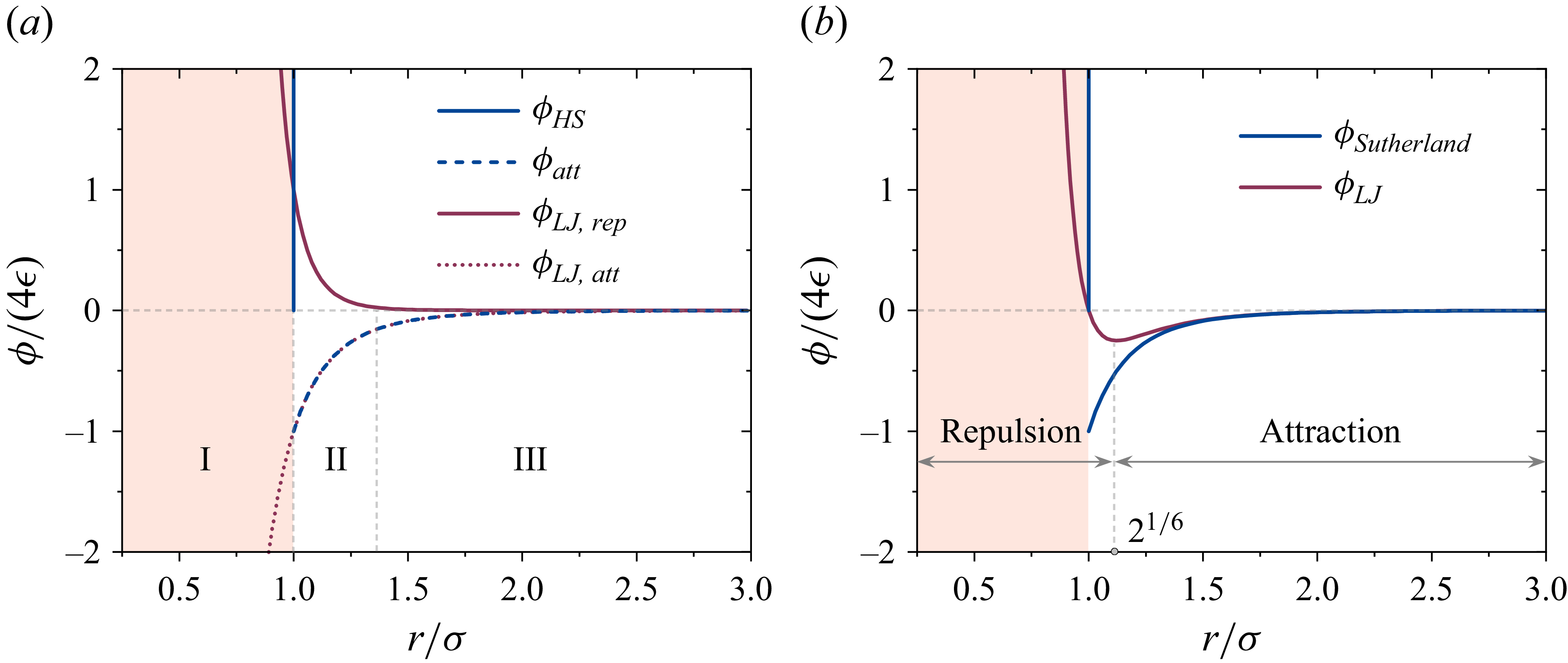
(a) The repulsive and attractive parts of the Lennard-Jones (LJ) and Sutherland potentials. (b) The overall LJ and Sutherland potentials.

By accounting for both the volume exclusion and molecular attraction, the Enskog–Vlasov (EV) equation and its model equations can resolve the structure of the liquid–vapour interface and describe the coexistence of liquid and vapour phases, whether they are dilute or dense, without requiring kinetic boundary conditions at the liquid–vapour interface (Frezzotti, Barbante & Gibelli Reference Frezzotti, Barbante and Gibelli2019; Li et al. Reference Li, Su, Shan, Li, Gibelli and Zhang2024; Struchtrup et al. Reference Struchtrup, Jahandideh, Couteau and Frezzotti2024). Consequently, the EV framework has been widely adopted to study non-equilibrium evaporation phenomena. Applications include e.g. the evaporation of a thin liquid film into a vacuum (Frezzotti et al. Reference Frezzotti, Gibelli and Lorenzani2005, Reference Frezzotti, Gibelli, Lockerby and Sprittles2018), the determination of kinetic boundary conditions at the interface (Frezzotti Reference Frezzotti2011; Kon, Kobayashi & Watanabe Reference Kon, Kobayashi and Watanabe2014; Kobayashi et al. Reference Kobayashi, Sasaki, Kon, Fujii and Watanabe2017), spinodal decomposition (Sadr, Pfeiffer & Gorji Reference Sadr, Pfeiffer and Gorji2021), and comparisons with MD simulations (Homes et al. Reference Homes, Frezzotti, Nitzke, Struchtrup and Vrabec2025). Related moment equations (Struchtrup & Frezzotti Reference Struchtrup and Frezzotti2022), lattice Boltzmann models (Hosseini, Dorschner & Karlin Reference Hosseini, Dorschner and Karlin2022) and simplified kinetic models (Takata, Matsumoto & Hattori Reference Takata, Matsumoto and Hattori2021; Miyauchi & Takata Reference Miyauchi and Takata2024) have also been developed for specific problems, reinforcing the generality of this framework. Recently, a molecular kinetic model was proposed to reduce the computational cost of the EV equation while maintaining high accuracy compared to DSMC results (Li et al. Reference Li, Su, Shan, Li, Gibelli and Zhang2024). In these studies, fluid molecules are described by a hard-sphere potential within a weak, attractive force field, yielding either the van der Waals (vdW) or Carnahan–Starling (CS) equation of state (EoS) in the hydrodynamic limit. However, this treatment has a fundamental drawback, rendering the EV-type models incapable of predicting accurate thermodynamic properties (Benilov & Benilov Reference Benilov and Benilov2019). Physically, the hard-sphere potential fails to capture two key features. First, as described by the repulsive part of the LJ potential, molecules experience a repulsive force in region II (see figure 1) before their collision cores come into contact. Second, the softness of real intermolecular potentials allows for a degree of mutual penetration upon collisions (Barker & Henderson Reference Barker and Henderson1976). Both of these effects are absent in the current EV framework.
The importance of these factors has been recognised in both statistical mechanics and thermodynamics. In liquid perturbation theory, the softness of collisions is accounted for by selecting an effective, temperature-dependent molecular diameter (Barker & Henderson Reference Barker and Henderson1967; Chandler & Weeks Reference Chandler and Weeks1970; Barker & Henderson Reference Barker and Henderson1976) and/or modifying the pair correlation function (Verlet & Weis Reference Verlet and Weis1972). Similarly, in a vdW-type EoS, a temperature-dependent molecular volume can be employed to account for the soft repulsion (Moshfeghian, Shariat & Maddox Reference Moshfeghian, Shariat and Maddox1988; Fitzgerald et al. Reference Fitzgerald, Sudibandriyo, Pan, Robinson and Gasem2003; Kalikhman, Kost & Polishuk Reference Kalikhman, Kost and Polishuk2010), although such approaches can introduce additional issues that limit their application (Kontogeorgis, Privat & Jaubert Reference Kontogeorgis, Privat and Jaubert2019). These two limitations together likely underpin a key deficiency of the vdW-type EoS, namely the assumption of a fixed critical compressibility factor for all fluids, which contradicts the substance-specific nature of this parameter. This shortcoming is then inherited by EV-based kinetic models. As a result, kinetic models built upon a hard-sphere potential, corresponding to a vdW-type EoS in the hydrodynamic limit, inevitably fall short in accurately predicting real-fluid thermodynamic behaviours. To mitigate this issue, recent studies have demonstrated that modifying the pair correlation function through an appropriate EoS can restore thermodynamic consistency of real fluids (Shan et al. Reference Shan, Su, Gibelli and Zhang2023; Huang & Wu Reference Huang and Wu2025; Li, Gibelli & Zhang Reference Li, Gibelli and Zhang2026).
The surface confinement also significantly alters the liquid evaporation process, leading to nanoscale behaviour that diverges from the classical evaporation theory (Liu et al. Reference Liu, Yang, Zou, Hu, Li, Tan, Miljkovic and Yang2025). The underlying mechanism is multifold. First, fluid–solid attraction induces a disjoining pressure, resulting in the formation of adsorbed and thin films near the solid surface (Narayanan, Fedorov & Joshi Reference Narayanan, Fedorov and Joshi2011) and an inhomogeneous system. Second, evaporation vastly complicates the three-phase contact line dynamics (Mehrizi & Wang Reference Mehrizi and Wang2018; Sprittles Reference Sprittles2024) governed by vapour–solid and liquid–solid interactions. Third, capillary pressure establishes a self-regulating liquid–vapour interface, where the curvature dynamically adjusts to balance the evaporative mass loss with the capillary liquid supply. This feedback mechanism affects the interfacial area and the overall evaporation rate (Narayanan et al. Reference Narayanan, Fedorov and Joshi2011; Lu, Narayanan & Wang Reference Lu, Narayanan and Wang2015; John et al. Reference John, Enright, Sprittles, Gibelli, Emerson and Lockerby2019). Finally, the reduced length scale of the confinement means that the kinetic region, i.e. the Knudsen layer, can occupy a significant portion of the vapour flow field (Frezzotti & Barbante Reference Frezzotti and Barbante2017; John et al. Reference John, Enright, Sprittles, Gibelli, Emerson and Lockerby2019), leading to a stronger non-equilibrium effect, thereby rendering its modelling particularly more challenging.
Evaporation from nanopores has been extensively studied in recent years through theoretical (Narayanan et al. Reference Narayanan, Fedorov and Joshi2011; Lu et al. Reference Lu, Narayanan and Wang2015; John et al. Reference John, Gibelli, Enright, Sprittles, Lockerby and Emerson2021), numerical (John et al. Reference John, Enright, Sprittles, Gibelli, Emerson and Lockerby2019; Li, Wang & Xia Reference Li, Wang and Xia2021; De Fraja et al. Reference De Fraja, Rana, Enright, Cooper, Lockerby and Sprittles2022) and experimental (Wilke et al. Reference Wilke, Barabadi, Lu, Zhang and Wang2017; Lu et al. Reference Lu, Kinefuchi, Wilke, Vaartstra and Wang2019) methods, driven by rapid advancements in nano-technologies. These studies have yielded valuable insights into the underlying mechanisms and influential factors, such as the nanopore size (Narayanan et al. Reference Narayanan, Fedorov and Joshi2011), meniscus shape (Hanks et al. Reference Hanks, Lu, Sircar, Salamon, Antao, Bagnall, Barabadi and Wang2018; John et al. Reference John, Enright, Sprittles, Gibelli, Emerson and Lockerby2019), non-equilibrium effect (Lu et al. Reference Lu, Narayanan and Wang2015; John et al. Reference John, Gibelli, Enright, Sprittles, Lockerby and Emerson2021; Li et al. Reference Li, Wang and Xia2021) and evaporation coefficient (John et al. Reference John, Enright, Sprittles, Gibelli, Emerson and Lockerby2019, Reference John, Gibelli, Enright, Sprittles, Lockerby and Emerson2021). However, existing models often rely on the coupling of different methods to model distinct flow regions, which requires oversimplified assumptions and introduces coupling uncertainties. In addition, near-equilibrium phase change models such as the Hertz–Knudsen model are often used, which require effective evaporation/condensation coefficients to describe complex non-equilibrium phase change. Furthermore, the influence of surface confinement is typically modelled via purely diffusive or reflective wall boundary conditions, thereby neglecting its critical role in causing fluid inhomogeneities.
In this work, we present a molecular kinetic model for confined evaporative flows that addresses the interplay between surface confinement and non-equilibrium phase change. The model provides a consistent description of both the liquid and vapour phases, not only offering a more accurate representation of thermodynamics and three-phase contact line dynamics, but also capturing non-equilibrium and real fluid effects. By appropriately modelling vapour–liquid–solid interactions, the proposed framework establishes a mesoscopic theoretical framework to advance our fundamental understanding of confined evaporation and associated contact line phenomena.
The remainder of the paper is organised as follows. In § 2, the molecular interactions and equilibrium thermodynamics are briefly introduced, which constitute the two limiting cases for developing a molecular kinetic model. The proposed model is then described in detail in § 3. Numerical simulations are provided in § 4, where the model’s performance is validated against the experimental and MD data. Furthermore, the evaporation-driven flows in nanochannels are investigated, revealing phenomena such as liquid-meniscus breakage and disappearance of liquid droplets in hydrophilic and hydrophobic nanochannels, respectively. Final conclusions are drawn in § 5.
2. Molecular perspective on limitations of classical thermodynamic models
Thermodynamic behaviours emerge as a collective manifestation of molecular interactions, which can be systematically linked through a mesoscopic kinetic description. This section provides a brief molecular-level perspective on such a connection. We first introduce the microscopic pair interactions represented by the 12–6 LJ potential, and then the macroscopic equilibrium thermodynamics described by the vdW-type EoS. These two viewpoints represent the limiting cases that underpin the construction of a consistent molecular kinetic model to be developed in § 3.
2.1. Microscopic description of molecular interactions
At the molecular scale, the behaviour of a fluid is governed by pairwise interactions between molecules. A widely used representation is the 12–6 LJ potential (figure 1), expressed as
 \begin{align} \phi _{\textit{LJ}}(r)= \mathop {\underbrace {4\epsilon \left (\frac {\sigma }{r}\right )^{12}}}\limits _{\phi _{LJ, {rep}}}\, \mathop {\underbrace {-\,4\epsilon \left (\frac {\sigma }{r}\right )^6}}\limits _{\phi _{LJ, {att}}}, \end{align}
where
 $r$
is the intermolecular distance, and
 $\sigma$
and
 $\epsilon$
are the characteristic length and energy parameters, respectively. This potential has been widely employed in MD simulations to investigate phase-change phenomena (Vorholz et al. Reference Vorholz, Harismiadis, Rumpf, Panagiotopoulos and Maurer2000; Maroo & Chung Reference Maroo and Chung2009), yielding results in close agreement with experiments. Because it captures essential features of real molecular interactions without invoking additional assumptions, the LJ potential often serves as a benchmark for testing and developing molecular or mesoscopic models. The insights drawn from this potential will later help to identify the intrinsic limitations of the vdW-type EoS and suggest possible routes for improvement, to be discussed in § 2.2.
2.2. Limitations in cubic EoS and empirical corrections
A cubic EoS, such as the vdW, Peng–Robinson (PR), Soave–Redlich–Kwong (SRK) and CS EoS with an attractive term, is widely used to describe fluid thermodynamics at equilibrium. These equations offer a good compromise between computational efficiency and simulation reliability. Unlike the ideal gas law, a cubic EoS takes both molecular volume and intermolecular attraction into account, enabling it to describe two-phase coexistence below the critical temperature using the Maxwell construction method, etc.
However, such an EoS inherently produces a fixed critical compressibility factor, whereas in reality this factor is substance-specific. For instance, the critical compressibility factors of vdW, PR, SRK and CS (with vdW attraction) EoS are 0.375, 0.307, 0.333 and 0.359, respectively, while the experimental values typically fall between 0.26 and 0.30. Consequently, the vdW-type EoS generally overestimates the critical compressibility and thus cannot accurately reproduce the thermodynamic properties of most real fluids.
Two main strategies have been proposed to overcome this limitation, namely the volume translation and the temperature-dependent co-volume approaches. The volume translation method has been recommended by Young, Pessoa & Ahón (Reference Young, Pessoa and Ahón2017) based on a comprehensive comparison. Here, we employ this approach to enhance the predictive accuracy of a vdW-type EoS for real fluids.
Taking the PR EoS as an example, its standard form reads
 \begin{align} \left. \begin{array}{l} P =\dfrac {nk_BT}{1-nV_0}-\frac {a\alpha n^2}{1+2nV_0-(nV_0)^2},\\[9pt]\alpha = \left [1+\left (0.37464+1.54226\omega -0.26992\omega ^2\right )\left (1-\sqrt {T_r}\right )\right ]^2, \end{array} \right \} \end{align}
where
 $P$
is the pressure,
 $n$
is the fluid number density,
 $k_B$
is the Boltzmann constant,
 $T$
is the temperature,
 $V_0=2\pi \sigma ^3/3$
is the co-volume,
 $a$
is a constant that characterises the mean attractive strength between fluid molecules,
 $T_r=T/T_c$
is the reduced temperature (with
 $T_c$
being the critical temperature), and
 $\alpha$
is a function of temperature measuring the temperature dependence of molecular attraction.
To further improve accuracy, a volume translation correction introduces a modified molecular volume
 $V_m$
as the third parameter, effectively shifting the predicted liquid volume to better match the experimental data. The shift parameter is defined as
 $s=V_m/V_0$
(Jhaveri & Youngren Reference Jhaveri and Youngren1988). Following the approach proposed by Shi, Li & Pang (Reference Shi, Li and Pang2018), the volume translated PR (VT-PR) EoS can be written as
 \begin{align} \left. \begin{array}{l} P =\frac {nk_BT}{1+(s-1)nV_0}-\frac {a\alpha n^2}{(1+snV_0)\left [1+(s+1)nV_0\right ] +nV_0\left [1+(s-1)nV_0\right ]},\\[12pt]V_m =\frac {Z_ck_BT_c}{P_c}\left \{A\exp \left [-\frac {(T_r-1)^2}{2B^2}\right ]+C\right \},\\[12pt]\alpha =T_r^{2(D-1)}\exp \left [E\left (1-T_r^{2D}\right )\right ], \end{array}\right \} \end{align}
where
 $Z_c$
is the compressibility factor of real fluids, and
 $A{-}E$
are substance-specific coefficients determined from the acentric factor
 $\omega$
(see table 1). Note that the
 $\alpha$
function used here (Le Guennec et al. Reference Le Guennec, Privat and Jaubert2016) differs from that in (2.2), though other choices (Lopez-Echeverry, Reif-Acherman & Araujo-Lopez Reference Lopez-Echeverry, Reif-Acherman and Araujo-Lopez2017) are also possible. When the shift parameter is
 $s=0$
, (2.3) introduces no volume translation and reduces to the original PR form (2.2). This correction improves the prediction of saturated liquid densities for both non-polar and weak-polar fluids. The resulting EoS (2.3) will be employed in § 3 to provide a more accurate description of thermodynamic properties within the molecular kinetic model.
Coefficients as functions of the acentric factor in (2.3).

Although the volume-translation technique can substantially improve the prediction of saturated densities and pressures for a cubic EoS, this correction does not resolve the fundamental limitations in describing strongly associating fluids, e.g. water. Since cubic formulations do not provide a physically accurate Helmholtz free energy or chemical potential for such fluids, more advanced formulations – e.g. GERG- and IAPWS-type equations, and statistical associating fluid theory (Wagner & Pruß Reference Wagner and Pruß2002; Kunz & Wagner Reference Kunz and Wagner2012; Wilhelmsen et al. Reference Wilhelmsen, Aasen, Skaugen, Aursand, Austegard, Aursand, Gjennestad, Lund, Linga and Hammer2017) – offer a significantly improved description of thermodynamic properties, which have been successfully and consistently used in the density-functional and diffuse-interface approaches (Llovell et al. Reference Llovell, Galindo, Blas and Jackson2010; Magaletti, Gallo & Casciola Reference Magaletti, Gallo and Casciola2021). Such Helmholtz-energy-based formulations provide a natural route for extending the present kinetic framework to strongly associating fluids, and will be considered in future work.
3. Molecular kinetic model for evaporation
In this section, we will develop a molecular kinetic model to describe the phase-change process based on the principle of thermodynamic consistency. Here, thermodynamic consistency (Widom Reference Widom1963; He & Doolen Reference He and Doolen2002) implies two essential requirements: (i) the thermodynamic behaviour of a non-equilibrium system recovers the equilibrium description in the hydrodynamic limit; and (ii) the thermodynamic descriptions at the microscopic, mesoscopic and macroscopic levels remain consistent.
3.1. Transport equation for confined evaporation
A molecular kinetic model for surface-confined flows that consistently accounts for molecular interactions between fluid and solid was recently proposed by Shan et al. (Reference Shan, Torrilhon, Guo and Zhang2025). The distinguishing feature of our model is the explicit inclusion of both fluid–fluid and fluid–surface interactions in the transport equation, enabling it to capture essential nanoscale phenomena such as strong inhomogeneity, slip velocity and temperature jump. In the present study, this framework is extended to describe surface-confined evaporation and condensation occurring within a flow domain
 $V$
, which can accordingly be written as
 \begin{align} \frac {\partial f}{\partial t}+\boldsymbol{\xi } \boldsymbol{\cdot }\boldsymbol{\nabla }f + \boldsymbol{a}_e \boldsymbol{\cdot }\boldsymbol{\nabla} _{\boldsymbol{\xi }} f=\varOmega _E+\varOmega _V+J_V,\quad \boldsymbol{r} \in V, \\[-10pt] \nonumber \end{align}
 \begin{align} f(\boldsymbol{\xi }_t, \xi _n)- f(\boldsymbol{\xi }_t, -\xi _n)=-\omega _m\left [f(\boldsymbol{\xi }_t, -\xi _n) - f_w^{eq}\right ], \quad \boldsymbol{r} \in \partial V, \\[10pt] \nonumber \end{align}
where
 $f=f(\boldsymbol{r}, \boldsymbol{\xi }, t)$
is the velocity distribution function (VDF) of a fluid molecule with velocity
 $\boldsymbol{\xi }$
at position
 $\boldsymbol{r}$
and time
 $t$
,
 $\boldsymbol{a}_e$
is the external acceleration,
 $\boldsymbol{\xi }_t$
and
 $\xi _n$
represent the tangential and normal components of the molecular velocity, respectively, and
 $\omega _m$
is the accommodation coefficient. The three source terms
 $\varOmega _E$
,
 $\varOmega _V$
and
 $J_V$
describe fluid–fluid volume exclusion, fluid–fluid molecular attraction, and fluid–solid molecular attraction, respectively, expressed as
 \begin{align} \varOmega _E \approx \varOmega _B+\varOmega _{ex}, \\[-10pt] \nonumber \end{align}
 \begin{align} \varOmega _V = m^{-1}\,\boldsymbol{\nabla }\phi _{\textit{ff}}\boldsymbol{\cdot }\boldsymbol{\nabla} _{\boldsymbol{\xi }}f, \\[-10pt] \nonumber \end{align}
 \begin{align} J_V = m^{-1}\, \boldsymbol{\nabla }\phi _{\textit{fs}}\boldsymbol{\cdot }\boldsymbol{\nabla} _{\boldsymbol{\xi }}f, \\[10pt] \nonumber \end{align}
where
 $\varOmega _B$
is the Boltzmann-type collision operator, and
 $\varOmega _{ex}$
is the excessive term. The macroscopic density and flow velocity fields are obtained from the velocity moments of the VDF, namely
 \begin{align} [n, n\boldsymbol{u}]=\int [f, \boldsymbol{\xi }f]\,\mathrm{d}\boldsymbol{\xi }. \end{align}
The operator
 $\varOmega _E$
in (3.1a
) for fluid–fluid interactions plays a dual role. First, it represents momentum and energy exchange during instantaneous molecular collisions, captured by the Boltzmann collision operator
 $\varOmega _B$
or its simplified forms, such as the Bhatnagar–Gross–Krook (BGK) model (Bhatnagar, Gross & Krook Reference Bhatnagar, Gross and Krook1954). Second, it accounts for the finite molecular size, which causes the centres of colliding molecules to be separated, and leads to the collisional transport of momentum and energy. With the BGK model and Enskog theory for isothermal dense fluids, these two terms can be written as
 \begin{align} \varOmega _B =-\tau _f^{-1}\left (f-f^{eq}\right ), \\[-10pt] \nonumber \end{align}
 \begin{align} \varOmega _{ex}=-V_0f^{eq}\, \boldsymbol{c}\boldsymbol{\cdot }(2\chi\, \boldsymbol{\nabla }n+ n\,\boldsymbol{\nabla }\chi ), \\[10pt] \nonumber \end{align}
where
 $\tau _f$
is the relaxation time, and
 $\boldsymbol{c}=\boldsymbol{\xi }-\boldsymbol{u}$
is the peculiar velocity. For thermal flows, (3.4a
) can be replaced by other kinetic models, e.g. the Shakhov model (Shakhov Reference Shakhov1968), to recover the correct Prandtl number. The equilibrium distribution functions for the fluid and the solid are
 \begin{align} f^{eq}=n(2\pi RT)^{-{3}/{2}}\exp \left (-\frac {|\boldsymbol{c}|^2}{2RT}\right )\!, \\[-10pt] \nonumber \end{align}
 \begin{align} f_w^{eq}=n_w(2\pi RT_w)^{-{3}/{2}}\exp \left (-\frac {|\boldsymbol{\xi }-\boldsymbol{u}_w|^2}{2RT_w}\right )\!, \\[10pt] \nonumber \end{align}
where
 $n_w$
is the fluid density at the effective boundary
 $\partial V$
, and
 $\boldsymbol{u}_w$
and
 $T_w$
are the velocity and temperature of the solid wall, respectively.
It is noted that the counterpart of
 $\varOmega _E$
in (3.1a
) that accounts for the fluid–surface interactions has been reduced to (3.1b
) serving as a non-local condition linking the fluid and the solid through molecular interactions. The effective boundary
 $\partial V$
is located at a distance
 $H_{ex}$
inside the flow domain from the physical boundary, where
 $H_{ex}$
can be estimated using the hard-sphere approximation and the Berthelot rule (Berthelot Reference Berthelot1898) as
 $H_{ex}=\sigma _{\textit{fs}}=(\sigma _{f}+\sigma _{s})/2$
, with the subscripts
 $f$
,
 $s$
and
 $fs$
representing the fluid, the solid, and their combination, respectively. Accordingly, the accommodation coefficient is expressed as
 \begin{align} \omega _m=\begin{cases} \dfrac {\bar {t}_{\textit{fs}}}{\tau _m},&\boldsymbol{r} \in \partial V, \\[6pt] 0,&\text{otherwise}, \end{cases} \end{align}
where
 $\bar {t}_{\textit{fs}}$
is the characteristic time for fluid–surface collisions, defined as the mean time between successive fluid–surface collisions, and representing how frequently fluid molecules interact with the solid. Meanwhile,
 $\tau _m$
is the relaxation time that quantifies the exchange rate of momentum and energy during fluid–surface collisions. Although both quantities have clear physical meanings, they represent molecular collective behaviours near the surface, and are difficult to determine in practice. Consequently, their ratio, defined as the accommodation coefficient, can be employed to characterise fluid–surface interactions, measuring the degree of equilibration achieved per collision. This coefficient depends on properties of fluids and solids, and is treated as a constant between 0 and 1 in the present study.
The attractive potentials between fluid–fluid and fluid–solid molecules are modelled as
 \begin{align} \phi _{\textit{ff}}(\boldsymbol{r})=\alpha \int _{|\boldsymbol{r}'|\gt \sigma _{\kern-1pt f}}n(\boldsymbol{r}+ \boldsymbol{r}')\,\phi _{\textit{att}}(\boldsymbol{r}')\,\mathrm{d}\boldsymbol{r}', \\[-10pt] \nonumber \end{align}
 \begin{align} \phi _{\textit{fs}}(y)=-2c_{\textit{ad}}n_D\pi \epsilon _{\textit{fs}}\left (\frac {\sigma _{\textit{fs}}}{y}\right )^4, \\[6pt] \nonumber \end{align}
where
 $\phi _{\textit{att}}=-4\epsilon _f(\sigma _{\kern-1pt f}/r)^6$
is the attractive part of the 12–6 LJ potential (2.1),
 $\phi _{\textit{fs}}$
is the attractive component of the 10–4 potential representing fluid–wall interactions,
 $\epsilon _{\textit{fs}}=\sqrt {\epsilon _f\times\epsilon _s}$
(Lorentz Reference Lorentz1881),
 $n_D$
is the reduced solid density, and
 $c_{\textit{ad}}$
is a coupling factor that controls the strength of fluid–solid attraction. It is noted that the
 $\alpha$
function is introduced in the mean-field force term, which is consistent with that used in the VT-PR EoS (2.3).
The mean-field modelling of molecular attraction, i.e. (3.7a ), is in its non-local convolution form, which implicitly contains high-order gradient contributions (Struchtrup & Frezzotti Reference Struchtrup and Frezzotti2022) compared to the square-gradient free energy description. Therefore, curvature-dependent interfacial effects, such as the Tolman-length corrections to the surface tension, are in principle embedded in this formulation. While such effects are not explicitly analysed in the present work, they can be studied by examining the curvature dependence of surface tension for spherical droplets or bubbles.
By contrast, the fluid–wall attraction (3.7b
) is treated locally in the present formulation. As a result, while density variations and interfacial structuring near solid surfaces are captured, the model does not reproduce the molecular-scale oscillation predicted by non-local density functional theories (Tarazona Reference Tarazona1985; Tarazona, Marconi & Evans Reference Tarazona, Marconi and Evans1987). Instead, the resulting interfacial structure is closer to that obtained from gradient-based free-energy descriptions (Talanquer & Oxtoby Reference Talanquer and Oxtoby1996; Gallo, Magaletti & Casciola Reference Gallo, Magaletti and Casciola2021). Nevertheless, whereas wettability in such gradient-based approaches is typically prescribed through a macroscopic contact angle, it emerges from microscopic fluid–surface interactions (3.7b
) in the present model, with the parameter
 $c_{\textit{ad}}$
controlling the strength of adhesion in a manner analogous to MD simulations. Therefore, the present kinetic model positions as an intermediate model linking fully microscopic approaches and continuum diffuse-interface theories.
3.2. Thermodynamic consistency and closure of the kinetic model
Here, we perform a thermodynamic consistency analysis and propose a new pair correlation function to close the molecular kinetic model. To ensure thermodynamic consistency, the molecular kinetic equation (3.1) is analysed using the Chapman–Enskog expansion (Chapman & Cowling Reference Chapman and Cowling1990), which recovers the macroscopic hydrodynamic equations under the Einstein summation convention as
 \begin{align} \partial _t \rho + \partial _i (\rho u_i)=0, \\[-10pt] \nonumber \end{align}
 \begin{align} \partial _t (\rho u_i)+\partial _j[P\delta _{\textit{ij}}-\varPi _{\textit{ij}}-K_{\textit{ij}}+\rho u_i u_j]-\rho a_i=0, \\[10pt] \nonumber \end{align}
where
 $\rho =mn$
is fluid density, with
 $m$
being the molecular mass,
 $\delta _{\textit{ij}}$
is the Kronecker delta function,
 $\boldsymbol{a} = \boldsymbol{a}_e-\boldsymbol{\nabla }\phi _{\textit{fs}}$
, and
 $\varPi _{\textit{ij}}$
and
 $K_{\textit{ij}}$
are the viscous and Korteweg-type stress tensors (Anderson, McFadden & Wheeler Reference Anderson, McFadden and Wheeler1998), respectively, defined as
 \begin{align} \varPi _{\textit{ij}}=nk_BT\tau _f \left [(\partial _i u_j+\partial _j u_i)-\frac {2}{3}\partial _k u_k\delta _{\textit{ij}}\right ], \\[-10pt] \nonumber \end{align}
 \begin{align} K_{\textit{ij}}=k \left [\left (n\,{\nabla} ^2n+\frac {1}{2}|\boldsymbol{\nabla }n|^2\right )\delta _{\textit{ij}}-\boldsymbol{\nabla }n\, \boldsymbol{\nabla }n\right ], \\[6pt] \nonumber \end{align}
where
 $k$
is a coefficient determined by the intermolecular potential. The pressure
 $P$
satisfies
 \begin{align} P=nk_BT(1+nV_0\chi )-a\alpha n^2, \end{align}
where the first term represents the repulsive interaction, and the second term represents the molecular attraction. Different from our previous kinetic models (Shan et al. Reference Shan, Su, Gibelli and Zhang2023; Li et al. Reference Li, Su, Shan, Li, Gibelli and Zhang2024), the present formulation introduces the temperature-dependent function
 $\alpha (T)$
as a consequence of (3.7a
) to account for the variation of attractive strength with temperature (Kontogeorgis et al. Reference Kontogeorgis, Privat and Jaubert2019).
When the attractive part of the 12–6 LJ potential is used, the coefficients
 $a$
and
 $k$
are obtained as
 \begin{align} a=-\frac {1}{2}\int _{r\gt \sigma _{\kern-1pt f}}\phi _{\textit{att}}(r)\,\mathrm{d}\boldsymbol r=\frac {8\pi \sigma _{\kern-1pt f}^3}{3}\epsilon _f, \\[-10pt] \nonumber \end{align}
 \begin{align} k=-\frac {1}{6}\int _{r\gt \sigma _{\kern-1pt f}}r^2\,\phi _{\textit{att}}(r)\,\mathrm{d}\boldsymbol r=\frac {8\pi \sigma _{\kern-1pt f}^5}{3}\epsilon _f. \\[6pt] \nonumber \end{align}
The Chapman–Enskog analysis thus provides: (i) the connection between the relaxation time and the shear viscosity; and (ii) the EoS linking the kinetic description to the equilibrium thermodynamics, as introduced in § 2. Furthermore, it establishes the correlations between macroscopic parameters (
 $V_0$
and
 $a$
) and molecular quanties (
 $\sigma _{\kern-1pt f}$
and
 $\epsilon _f$
), which is essential for constructing a physically consistent molecular kinetic model.
By comparing (3.9a ) with Newton’s law of viscosity, the relaxation time is expressed as
 \begin{align} \tau _f(y) = \frac {\mu _s(y)}{n(y)\,k_BT}, \end{align}
where
 $\mu _s$
is the shear viscosity of real fluids, which can be obtained from MD simulations, theoretical/empirical formulas, or experimental measurements (Shan et al. Reference Shan, Torrilhon, Guo and Zhang2025). Since the viscosity plays an important role in the kinetic model through the relaxation process, more accurate viscosity models lead to better predictions. Here, we use the semi-empirical formulation reported in Chung et al. (Reference Chung, Ajlan, Lee and Starling1988) to determine the viscosity of both vapour and liquid phases. Due to density and viscosity oscillations, the relaxation rates of fluids in the bulk and near the solid surface are intrinsically different.
Classical cubic EoS, such as the vdW, PR, SRK and CS (with an attraction term) equations, often fail to reproduce the vapour–liquid equilibrium coexistence curve of LJ fluids such as argon accurately, particularly near the critical temperature and pressure. For a more accurate representation of equilibrium thermodynamic properties, the pair correlation function
 $\chi$
in (3.10) is calibrated using the VT-PR EoS (2.3), which can be decomposed as
 \begin{align} \begin{split} P&= \mathop {\underbrace {\frac {nk_BT}{1+(s-1)nV_0}}}\limits _{\text{hard repulsion}} - \mathop {\underbrace {a\alpha n^2}}\limits _{\text{attraction}}\\ &\quad{}+ \mathop {\underbrace {a\alpha n^2\left \{1-\frac {1}{(1+snV_0)[1+(s+1)nV_0]+nV_0[1+(s-1)nV_0]} \right \}}}\limits _{\text{soft repulsion modification}}. \end{split} \end{align}
The first two terms represent the hard-sphere repulsion and molecular attraction, respectively, while the third term represents a correction due to the soft repulsion arising from the finite softness of the molecular core (Abbott & Prausnitz Reference Abbott and Prausnitz1987; Nezbeda, Melnyk & Trokhymchuk Reference Nezbeda, Melnyk and Trokhymchuk2010; Kontogeorgis et al. Reference Kontogeorgis, Privat and Jaubert2019). Physically, as illustrated in figure 1, the repulsive part of the LJ potential decays rapidly in the near-contact region (
 $r/\sigma \approx 1$
in regions I and II), whereas the idealised hard-sphere potential acts only at instantaneous collision. The soft repulsion correction therefore compensates for this discrepancy. Since the repulsive interactions primarily influence the collision dynamics, they enter the kinetic model through the pair correlation function
 $\chi$
, which consequently becomes temperature-dependent. With these considerations, the pair correlation function is determined as
 \begin{align} \left. \begin{array}{l} \chi = \frac {1-s}{1+(s-1)nV_0} + \frac {a\alpha n}{k_BT}\frac {\hat {s}}{1+\hat {s}nV_0}, \\[14pt] \hat {s} = 2(s+1) +(s^2+2s-1)nV_0, \end{array}\right \} \end{align}
according to the modified Enskog theory (Chapman & Cowling Reference Chapman and Cowling1990).
To maintain thermodynamic consistency between the molecular and macroscopic descriptions, the vdW constants
 $V_0$
and
 $a$
should be linked to the critical properties (
 $T_c$
,
 $P_c$
and
 $V_c$
) and the molecular characteristics (
 $\sigma _{\kern-1pt f}$
and
 $\epsilon _f$
). Because the critical volume
 $V_c$
is often less accurately known, it is preferable to relate vdW constants directly to the critical pressure
 $P_c$
and temperature
 $T_c$
. At the critical point, the following conditions apply:
 \begin{align} \frac {\partial P}{\partial n}=0\quad \text{and}\quad \frac {\partial ^2 P}{\partial n^2}=0. \end{align}
From these relations, the PR EoS and VT-PR EoS yield
 \begin{align} V_0 =0.07780\frac {k_BT_c}{P_c}, \quad a=0.45724\frac {(k_BT_c)^2}{P_c}. \end{align}
The co-volume and attraction parameters can thus be connected to the molecular parameters using
 $V_0=2\pi \sigma ^3/3$
and (3.11a
), giving
 \begin{align} \sigma _{\kern-1pt f}=\left (\frac {0.11670}{\pi }\frac {k_BT_c}{P_c}\right )^{{1}/{3}}, \quad \epsilon _f = 1.46928k_B T_c. \end{align}
Analogous relations between molecular and critical parameters, as well as the corresponding expressions for pair correlation function
 $\chi$
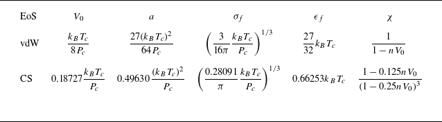
, can be derived for the vdW EoS and CS EoS. These are summarised in table 2 for later comparison.
Relationship between molecular interaction parameters, critical properties, and the pair correlation function for the vdW EoS and CS EoS.

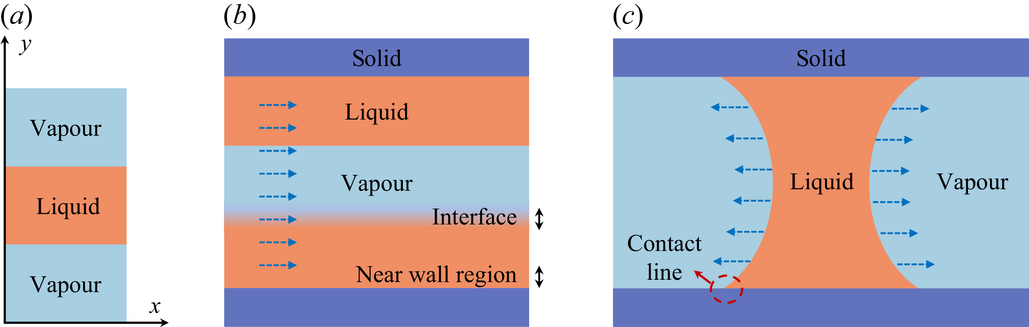
Configuration of (
 $a$
) vapour–liquid equilibrium without presence of solid surface, (
 $b$
) surface-confined force-driven evaporative flows, and (
 $c$
) surface-confined evaporation-driven liquid–vapour flows. Dashed arrows represent the flow direction.

4. Results and discussion
In this section, we first present the numerical results of the present molecular kinetic model for vapour–liquid equilibrium and surface-confined force-driven evaporative flows, as illustrated in figures 2(
 $a$
) and 2(
 $b$
), respectively. Where appropriate, comparisons are made with MD simulations or experimental data to demonstrate the capability of the present model in capturing fluid adsorption, liquid–vapour interfaces and velocity slip. We then apply the model to study surface-confined evaporation-driven liquid–vapour flows, as shown in figure 2(
 $c$
), a configuration for which MD simulations are prohibitively expensive because of the slow and unsteady dynamics (Fan et al. Reference Fan, Wu and Wang2020b
).
4.1. Numerical methods
Argon is selected as the working fluid (except in figure 3
 $b$
) owing to its simple structure and well-characterised intermolecular potential, which enables accurate reproduction of its thermodynamic properties (Rahman Reference Rahman1964; Fan et al. Reference Fan, Wu and Wang2020b
). The energy and length parameters are selected to ensure that the critical pressure and temperature are consistent in the MD and kinetic simulations. In the MD simulations, the molecular length and energy parameters are
 $\sigma _{\kern-1pt f} =0.3405$
nm and
 $\epsilon _f =0.237949$
kcal mol
 $^{-1}$
, respectively. In the molecular kinetic model, these parameters are instead determined by the critical pressure and temperature (
 $P_c = 4.863$
MPa and
 $T_c=150.687$
K for argon) using (3.17) and table 2, depending on the choice of the pair correlation function and EoS. This selection ensures that both approaches yield consistent thermodynamic conditions.
In MD simulations, the solid substrate is modelled as a face-centred-cubic crystal with lattice spacing 0.4065 nm, and the molecular length and energy parameters, i.e.
 $\sigma _w=0.3293$
nm and
 $\epsilon _w=0.039000$
kcal mol
 $^{-1}$
. Each solid molecule is tethered to its lattice site via a linear spring potential. The Lorentz–Berthelot mixing rules (Lorentz Reference Lorentz1881; Berthelot Reference Berthelot1898) are used to determine the mixed energy and length parameters. The interactions between argon and solid molecules are modelled by the 12–6 LJ potential with cut-off distance 2.5 nm. Although a smaller cut-off distance accelerates computation, it may fail to produce convergent solutions. The Nosé–Hoover thermostat is applied to maintain the temperature of both argon and substrate. Molecular trajectories are integrated by solving Newton’s equation of motion with time step 0.5 fs under periodic boundary conditions in all directions. All MD simulations are performed using the large-scale atomic/molecular massively parallel simulator (Thompson et al. Reference Thompson2022).
The present molecular kinetic model is solved using the discrete unified gas kinetic scheme (Guo, Xu & Wang Reference Guo, Xu and Wang2013; Zhang et al. Reference Zhang, Zhu, Wang and Guo2018), which is applicable to both continuum and non-equilibrium flows. The method has recently been extended to strongly inhomogeneous flows (Shan et al. Reference Shan, Wang, Zhang and Guo2020), where fluid–solid interactions become significant. In this work, the fluid–solid interactions are treated following the approach presented in Shan et al. (Reference Shan, Torrilhon, Guo and Zhang2025), in which the force field and momentum exchange between fluids and solids are consistently taken into account in the transport (3.1). A cut-off distance 2.5 nm is adopted in calculating the molecular attraction according to (3.7), which is consistent with that in MD simulations, and sufficiently large to ensure convergence. For liquid–vapour equilibrium (figure 2
 $a$
) and confined force-driven flows (figure 2
 $b$
), the flow field varies only in the
 $y$
direction, allowing the VDF to be integrated over
 $\xi _x$
and
 $\xi _z$
planes. In contrast, for the evaporation-driven liquid–vapour flows (figure 2
 $c$
), variations occur in both the
 $x$
and
 $y$
directions, and the VDF is integrated only over
 $\xi _z$
. Correspondingly, the mean-field force term should be reduced to one- and two-dimensional spaces, with the details given in Appendix A.
Comparison of the vapour–liquid equilibrium properties for (
 $a$
) argon and (
 $b$
) carbon dioxide. Here, PR, CS and vdW denote the respective EoS, with vapour–liquid coexistence properties obtained from the Maxwell construction. The EV-CS results are computed using the present framework coupled with the CS EoS. The MD data for carbon dioxide are taken from Vorholz et al. (Reference Vorholz, Harismiadis, Rumpf, Panagiotopoulos and Maurer2000).

4.2. Vapour–liquid equilibrium
The liquid–vapour coexistence curves are compared to assess whether the present kinetic model improves predictive accuracy and captures the structure of the liquid–vapour interface. In figure 3(
 $a$
), the coexistence curves for the PR EoS and vdW EoS are determined using the Maxwell equal-area construction, while the CS EoS employs the thermodynamic equilibrium criterion (Frezzotti et al. Reference Frezzotti, Gibelli, Lockerby and Sprittles2018), which requires equal pressure and chemical potential in two phases. The experimental data (Tegeler, Span & Wagner Reference Tegeler, Span and Wagner1999) and MD results (Maroo & Chung Reference Maroo and Chung2009) are included for comparison. In our kinetic simulations, a liquid slab of height
 $h_l=3H/7$
is confined between two vapour regions of height
 $h_v=2H/7$
, with the periodic boundary condition applied in the
 $y$
direction. As shown in figure 3(
 $a$
), the present kinetic model reproduces liquid–vapour coexistence accurately from low to near-critical temperatures. By contrast, the PR EoS and CS EoS overestimate liquid densities at low temperatures, whereas the vdW EoS significantly underestimates them across the entire temperature range.
Figure 3(
 $b$
) shows the predicted liquid–vapour coexistence curve for carbon dioxide (CO
 $_2$
), with the experimental data (Span & Wagner Reference Span and Wagner1996) and MD results (Vorholz et al. Reference Vorholz, Harismiadis, Rumpf, Panagiotopoulos and Maurer2000) serving as the benchmark data. The relevant critical properties are
 $P_c=7.38$
MPa,
 $T_c=304.13$
K, and the acentric factor
 $\omega =0.22394$
. The kinetic model again provides accurate predictions across the studied temperature range, whereas the EV equation employing a pair correlation function derived from the CS EoS overestimates the vapour density. Surprisingly, the difference in the predicted liquid densities for CO
 $_2$
is minor, indicating a more accurate description of liquid CO
 $_2$
than the monatomic liquid argon.
Comparison of vapour and liquid (argon) distribution at (
 $a$
) 105 K, (
 $b$
) 130 K and (
 $c$
) 140 K.

The MD simulations are further performed to evaluate the accuracy of the kinetic model in capturing the structure of the liquid–vapour interface across different temperatures, as shown in figure 4. The upper and lower dashed lines denote the experimental liquid and vapour densities (Tegeler et al. Reference Tegeler, Span and Wagner1999), respectively. At low (
 $T=105$
K, figure 4
 $a$
) and intermediate (
 $T=130$
K, figure 4
 $b$
) temperatures, the kinetic model reproduces both the interfacial structure and the equilibrium density with good accuracy. Near the critical temperature (
 $T=140$
K), some discrepancies arise between the kinetic model and MD predictions due to the modelling challenges arising from the complex fluid properties.
The kinetic model is more accurate in describing the vapour phase than the MD simulation, while the kinetic model and MD simulation slightly underestimate and overestimate the liquid density, respectively. Overall, the agreement between the kinetic model and MD simulations remains satisfactory across the examined temperature range.
4.3. Model comparison for pressure calculation
In the molecular kinetic model, the pressure is evaluated by (3.10), which depends on the choice of the pair correlation function, and hence the EoS recovered in the hydrodynamic limit. We compare here the predicted pressure of argon using different forms of the pair correlation function, corresponding to the vdW, CS, PR and VT-PR EoS. The experimental results (Tegeler et al. Reference Tegeler, Span and Wagner1999) are used as the benchmark data.
Figure 5 shows the variation of pressure with density at different temperatures. In figures 5(
 $a$
,
 $b$
), a nearly constant-pressure region appears where the density increases markedly, corresponding to the liquid–vapour transition, whereas figure 5(
 $c$
) represents the supercritical regime. At low densities, all models predict accurate pressures because real fluid effects are not significant. Below the critical temperature, the CS and VT-PR models respectively overestimate and underestimate the liquid pressure, yet both perform better than the vdW and PR models, as shown in figures 5(
 $a$
,
 $b$
). In the supercritical regime, the VT-PR model provides the most accurate prediction, maintaining good agreement with the experimental data up to pressure
 $P=100.0$
MPa. Although the volume translation technique substantially improves the accuracy of liquid density predictions, some discrepancies persist at elevated pressures and near the critical temperature. These discrepancies stem from the intrinsic limitations of the cubic EoS, which links to the kinetic model through the pair correlation function and the mean-field attractive term. Adopting a more accurate EoS therefore offers a potential route to further reduce these deviations.
Since the discrepancies among the models are most pronounced at large densities, we further examine the variation of pressure and pair correlation function with temperature at
 $\rho =750.0$
kg m
 $^{-3}$
in figures 6(
 $a$
,
 $b$
), and
 $\rho =1000.0$
kg m
 $^{-3}$
in figures 6(
 $c$
,
 $d$
). The VT-PR model yields the most accurate pressure at both densities, followed by the PR model. This result supports the validity of the proposed pair correlation function (3.14) and the inclusion of the
 $\alpha$
-function in the mean-field term to account for molecular attraction in a physically realistic manner (Kontogeorgis et al. Reference Kontogeorgis, Privat and Jaubert2019). As the temperature rises, perturbation theory for liquids (Barker & Henderson Reference Barker and Henderson1967; Karkheck & Stell Reference Karkheck and Stell1981) introduces a temperature-dependent reduction of the hard-core volume to represent the softening of repulsive interactions, equivalently corresponding to a smaller hard-core diameter and thus a lower pair correlation function value. As shown in figures 6(
 $b$
,
 $d$
), this decreasing trend is correctly captured by the VT-PR and PR models, but not by the vdW and CS formulations.
In the perturbation theory of liquids (Barker & Henderson Reference Barker and Henderson1976), the temperature-dependent hard-core diameter
 $\sigma _{pb}$
is related to the LJ diameter
 $\sigma _{\textit{LJ}}$
through (Cotterman, Schwarz & Prausnitz Reference Cotterman, Schwarz and Prausnitz1986)
 \begin{align} \frac {\sigma _{pb}}{\sigma _{\textit{LJ}}} = \int _{0}^{1}\left \{1-\exp \left [\frac {\phi _{\textit{LJ}}(\hat {r})}{k_BT}\right ]\right \} \mathrm{d}\hat {r} \approx \frac {1+0.29770T_r}{1+0.33163T_r+0.001047T_r^2}, \end{align}
where
 $T_r=k_BT/\epsilon _f$
, and
 $\hat {r}$
is the intermolecular centre-to-centre distance normalised by
 $\sigma _{\textit{LJ}}$
. Using this relation, the pair correlation function for the LJ fluids can be obtained with the hard-sphere approximation (Barker & Henderson Reference Barker and Henderson1967). Applying this perturbation technique to the vdW EoS markedly improves its pressure prediction, as shown in figures 6(
 $a$
,
 $c$
), particularly at
 $\rho =750.0$
kg m
 $^{-3}$
, although noticeable discrepancies remain at
 $\rho =1000.0$
kg m
 $^{-3}$
. As shown in figures 6(
 $b$
,
 $d$
), the pair correlation function obtained from the perturbed vdW EoS decreases slightly with temperature, reflecting the softening of intermolecular collisions in a manner consistent with our proposed model.
The prediction of pressure at different densities under constant temperatures (
 $a$
) 120.0 K, (
 $b$
) 145.0 K and (
 $c$
) 200.0 K.

The variation of pressure and pair correlation function with temperature at densities (
 $a$
,
 $b$
) 750.0 kg m
 $^{-3}$
and (
 $c$
,
 $d$
) 1000.0 kg m
 $^{-3}$
.

In this section, pressure is evaluated only in the homogeneous vapour and liquid phases, where it is uniquely defined. Within the liquid–vapour interface, density gradients give rise to an anisotropic Korteweg-type stress tensor, and surface tension arises from the difference between the normal and tangential stresses. In the hydrodynamic limit, the Korteweg stress can be recovered from the EV-type kinetic model (Giovangigli Reference Giovangigli2020; Struchtrup & Frezzotti Reference Struchtrup and Frezzotti2022), thereby providing a microscopic foundation for the continuum description by linking the gradient coefficient
 $k$
to the molecular interaction parameters (
 $\sigma _{\kern-1pt f}$
and
 $\epsilon _f$
), as shown in (3.11).
4.4. Surface-confined force-driven evaporative flow
Surface confinement strongly influences flow behaviours, as it induces fluid inhomogeneity and interfacial slip (Shan et al. Reference Shan, Wang, Wang, Zhang and Guo2022; Corral-Casas et al. Reference Corral-Casas, Chen, Borg and Gibelli2024). The liquid–vapour coexistence further complicates these effects. Here, we study the force-driven evaporative flows in a confined geometry, as illustrated in figure 2(
 $b$
). The liquid and vapour molecules are driven by an external body force
 $G$
in the
 $x$
direction, while the confinement space
 $H$
denotes the distance between the innermost layer of solid walls in the
 $y$
direction. Unless otherwise stated, the simulations are performed at fixed temperature
 $T=130.0$
K, and the momentum accommodation coefficient is
 $\omega _m=0.85$
for both the liquid and vapour phases.
The density and velocity distributions of surface-confined evaporative flow: (
 $a$
,
 $b$
) a liquid slab sandwiched by two vapour regions, with
 $G=0.000006$
kcal mol
 $^{-1}$
Å
 $^{-1}$
and
 $H=40.0$
nm; (
 $c$
,
 $d$
) a vapour slab sandwiched by two liquid regions, with
 $G=0.000015$
kcal mol
 $^{-1}$
Å
 $^{-1}$
and
 $H=40.0$
nm; (
 $e$
,
 $f$
) the liquid and vapour slabs each occupy half of the channel, with
 $G=0.000025$
kcal mol
 $^{-1}$
Å
 $^{-1}$
and
 $H=20.0$
nm.

Figure 7 shows that fluid adsorption arises naturally from the fluid–solid interactions under surface confinement. The present molecular kinetic model captures the vapour adsorption well, but exhibits some deviation in predicting the multi-layer adsorption in the liquid phase. This limitation stems from the simplified treatment of the fluid–solid attraction in (3.7b ). A more rigorous description based on the density functional theory as developed in our previous studies (Guo, Zhao & Shi Reference Guo, Zhao and Shi2006; Shan et al. Reference Shan, Wang, Wang, Zhang and Guo2022) may improve the prediction but at a larger computational cost. Since the first adsorption layer, which dominates the momentum transfer between fluids and solids, is well captured for both phases, the simplified model strikes a good balance between modelling accuracy and computational efficiency. Away from the surface-dominated region, a well-defined liquid–vapour coexistence zone forms, where the molecular kinetic model agrees with the MD results, including the bulk liquid/vapour densities and the interfacial structure.
The comparison of velocity profiles between the molecular kinetic model and MD simulations reveals larger discrepancies than those observed for the density distribution. Specifically, the kinetic model tends to underestimate the vapour velocity and overestimate the liquid velocity, as shown in figures 7(
 $b$
) and 7(
 $d$
). These differences likely originate from the limitations of the mean-field approximation at low temperatures, where molecular correlations become pronounced and a mean-field treatment becomes less accurate. Interestingly, when considering an evaporating configuration in which the liquid and vapour each occupy half of the channel (figure 7
 $e$
), these opposing errors largely cancel each other, leading to a close match between the kinetic and MD velocity profiles, as illustrated in figure 7(
 $f$
).
4.5. Surface-confined evaporation-driven flows
When a liquid–vapour interface meets a solid boundary, a three-phase contact line forms. Here, we consider a nanochannel initially filled with a central liquid slab bounded by the vapour regions at the two open ends, as illustrated in figure 2(
 $c$
). Each vapour region is connected to an open reservoir, where the gas molecular distribution is described by the Maxwellian distribution function with a reduced vapour density
 $n_\infty$
and a drift vapour velocity
 $\boldsymbol{u}_\infty$
, i.e.
 \begin{align} f_\infty (\boldsymbol{\xi }_i) = n_\infty \left (2\pi RT_\infty \right )^{-{3}/{2}} \exp \left (-\frac {|\boldsymbol{\xi } - \boldsymbol{u}_\infty |^2}{2RT_\infty }\right ),\quad \boldsymbol{\xi }_i\boldsymbol{\cdot }\boldsymbol{n} \gt 0. \end{align}
The evolution of density in the
 $x$
direction at
 $y=H/2$
: (
 $a$
) hydrophilic nanochannel; (
 $b$
) hydrophobic nanochannel.

The simulation domain has dimensions length
 $L=21.0$
nm (
 $x$
direction) and height
 $H=7.0$
nm (
 $y$
direction), maintained at temperature
 $T=135.0$
K. The liquid slab, with initial density
 $\rho _l=1012.0$
kg m
 $^{-3}$
, occupies the region from
 $1L/4$
to
 $3L/4$
, while the remaining space is filled with vapour of density
 $\rho _v=135.0$
kg m
 $^{-3}$
. The open reservoir conditions are specified by the reduced density
 $\rho _\infty =68.0$
kg m
 $^{-3}$
and the drift velocity
 $|\boldsymbol{u}_\infty |=15.0$
m s
 $^{-1}$
in the
 $x$
direction. The open reservoir fills with undersaturated vapour, which acts as a sink that creates a net outflow of vapour molecules. The consequent reduction in local vapour pressure draws liquid from the core of the channel, sustaining a capillary flow from the liquid slab towards the vapour region to compensate for the evaporative mass loss.
Evaporation-driven liquid–vapour flows are investigated at different surface wettabilities, characterised by the fluid–solid coupling factors
 $c_{\textit{ad}}=3.0$
(hydrophilic) and
 $c_{\textit{ad}}=0.05$
(hydrophobic). Figures 8(
 $a$
,
 $b$
) show the temporal evolution of the fluid density along the channel centreline (
 $y=H/2$
), where only the right-hand half is displayed owing to the symmetry of the configuration. The liquid density in the hydrophilic channel is lower than that in the hydrophobic case, because more liquid molecules are adsorbed into the near-surface region due to the disjoining pressure. Initially, the bulk liquid and vapour coexist, with a sharp density gradient near the outlet as a result of the open reservoir boundary. As evaporation proceeds, the liquid region gradually contracts while the vapour region expands. The liquid bulk vanishes at a critical time, which is approximately
 $t=0.61$
ns for the hydrophilic channel, and
 $t = 1.60$
ns for the hydrophobic channel. The underlying mechanisms, however, differ with wettability, as discussed below.
Density contour in the (
 $a{-}e$
) hydrophilic and (
 $f{-}j$
) hydrophobic nanochannels, for times (
 $a$
–
 $e$
)
 $t=0.00$
,
 $0.01$
,
 $0.03$
,
 $0.47$
,
 $0.67$
ns, respectively, and (
 $f$
–
 $j$
)
 $t =0.00$
,
 $0.02$
,
 $0.52$
,
 $1.40$
,
 $1.76$
ns, respectively.

The distinct confinement characteristics lead to different meniscus evolution behaviours, as illustrated in figure 9. In the hydrophilic confinement (figures 9
 $a{-}e$
), the strong liquid–solid adhesion, surpassing the liquid cohesive force, enhances surface wetting, so liquid molecules are pulled to the solid surface to form an adsorbed film and a concave meniscus. Since liquid molecules are more stable at the liquid–solid interface, it becomes kinetically hindered to replenish the evaporating liquid at the centreline region. This inefficient mass transfer ultimately leads to the meniscus rupture at a critical point (see figure 9
 $e$
), when molecular cohesion overcomes the momentum input from non-local liquid–vapour collisions (Frezzotti & Gibelli Reference Frezzotti and Gibelli2008). By contrast, for the hydrophobic channel (figures 9
 $f{-}j$
), liquid cohesion prevails over adhesion. Hence the liquid de-wets from the solid surface, forming a convex meniscus, and creating a vapour gap near the wall. Liquid molecules near the liquid–vapour interface are in a higher energy state thus are more prone to evaporate than those in the bulk. Consequently, the convex meniscus evolves into an isolated droplet, as shown in figure 9(
 $i$
). The liquid molecules at the droplet centre are the most stable and last to evaporate, after which the droplet disappears and no liquid exists (figure 9
 $f$
). The dependence of the density field on wettability is consistent with MD results (Bucior, Yelash & Binder Reference Bucior, Yelash and Binder2009), supporting the validity of our fluid–surface interaction model. However, the predicted density profiles exhibit weaker oscillations than the MD results due to the local treatment of fluid–surface interactions, which neglects non-local packing effects. Such non-local correlations can be taken into account through the local average density method (Tarazona et al. Reference Tarazona, Marconi and Evans1987) to recover the density oscillation and disjoining pressure quantitatively in nano-confined flows, as demonstrated in our recent work (Shan et al. Reference Shan, Torrilhon, Guo and Zhang2025). This extension improves interfacial accuracy at the expense of increased computational cost, and will be pursued in future studies.
At the nanoscale, defining a precise contact angle becomes difficult because of the finite thickness of the liquid–vapour interface and the oscillatory density near the contact line, as is evident in figure 9. This observation highlights the necessity of multiscale modelling to capture such interfacial phenomena. The proposed kinetic model takes essential molecular-level interactions into account, and asymptotically recovers the continuum hydrodynamic limit, thereby offering a framework for understanding contact line dynamics and guiding the design of nanoscale evaporative cooling technologies. In the present kinetic model, interfacial friction and viscous dissipation are not introduced through explicitly prescribed friction coefficients or contact angles (Zhang et al. Reference Zhang, Guo, Seveno and De Coninck2023), but emerge implicitly from the microscopic fluid–surface interactions. Wettability is controlled by the fluid–surface attraction strength, which modifies the near-wall density structure and thereby affects momentum and energy exchange rates through fluid–surface collision dynamics governed by the accommodation coefficient. These density variations further lead to spatially varying transport properties, resulting in different viscous dissipation rates in the bulk fluids via Enskog collision dynamics. Consequently, interfacial friction and dissipation depend on wettability through the microscopic structure of fluids. While no explicit friction parameter is introduced, an effective friction coefficient could in principle be extracted from the resulting velocity and stress fields, providing a bridge between molecular interactions and continuum descriptions of dynamic wetting.
The evaporation flux in nanochannels is strongly influenced by the curvature of the liquid–vapour interface and by the slip velocity at the solid surface. Here, we compare the evaporation flux between hydrophilic and hydrophobic nanochannels. In the present configuration, the evaporation flux
 $J$
occurs only in the
 $x$
direction, and is obtained from the local density and velocity distributions at the channel outlet, namely
 \begin{align} J(y)=\rho (y)\,u_x(y). \end{align}
The evaporation fluxes immediately before meniscus rupture and droplet disappearance, respectively corresponding to
 $t=0.47$
ns and
 $t=1.40$
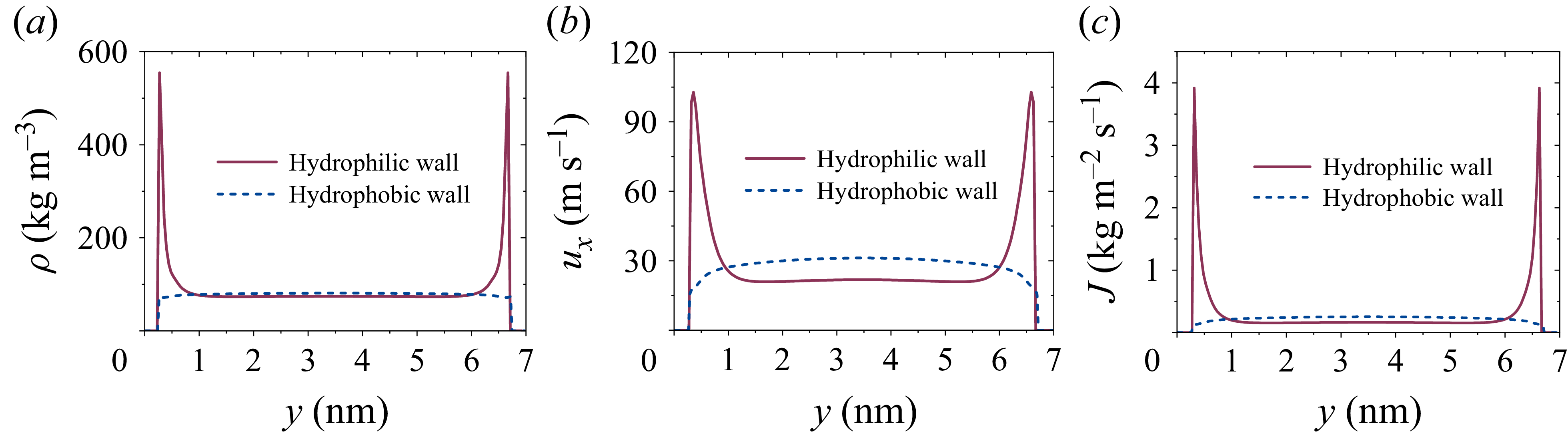
ns in figure 8, are examined for hydrophilic and hydrophobic confinements. The density, velocity and mass flux distributions at the right-hand outlet are shown in figure 10. In hydrophilic nanochannels, a pronounced density peak arises near the surface owing to the disjoining pressure, accompanied by an enhanced velocity in the thin film region caused by the large potential gradient. By contrast, in hydrophobic nanochannels, the density remains nearly uniform, and the velocity profile is only weakly developed, displaying slower velocities near the wall. Consequently, the mean evaporation flux, defined as
 $J_{avg}=\int _{0}^{H}J(y)\,\mathrm{d}y/H$
, is substantially higher in hydrophilic confinements (
 $2911.36$
kg m−2 s−1) than in hydrophobic ones (
 $2077.84$
kg m−2 s−1). The enhancement in the hydrophilic case arises primarily from the contact line region, as shown in figure 10(
 $c$
), where the combined effects of extended interfacial curvature, elevated density and velocity within the film, and slip at the wall, collectively promote evaporation.
The comparison of (
 $a$
) density, (
 $b$
) velocity and (
 $c$
) mass flux distributions of the evaporation-driven capillary flow in hydrophilic and hydrophobic nanochannels.

5. Conclusions
We have presented a molecular kinetic model for surface-confined evaporative flows that consistently considers the vapour–liquid–solid molecular interactions. Therefore, this model can directly address the interplay between evaporation and surface confinement. A key feature of the model is the automatic emergence of vapour–solid, liquid–solid and liquid–vapour interfaces, eliminating the need to couple different flow regions and to use a phase change model with ad hoc evaporation/condensation coefficients. Furthermore, the kinetic model captures the non-equilibrium effect within the Knudsen layer and vapour, as well as the real fluid effects in liquid and dense vapour, which reduce to the Boltzmann-type kinetic descriptions in the low pressure limit, and recover the hydrodynamic behaviours at larger spatial scales.
In the proposed model, the soft-collision effects in the pair correlation function and a temperature-dependent correction in the mean-field Vlasov term are considered to improve the predictive accuracy for pressure and liquid–vapour equilibrium properties, as validated against the experimental data and/or MD simulations. The model’s performance in simulation of surface-confined evaporative flows has been assessed against MD simulations, confirming its capability in capturing the fluid inhomogeneity and non-equilibrium evaporation. While some discrepancies in the velocity profiles are observed, the overall agreement is satisfactory. The discrepancies may be attributed to the known limitations of the mean-field theory at low temperatures where molecular correlations become significant. A further application to evaporation-driven capillary flows in nanochannels reveals the influence of surface wettability, and unravels underlying mechanisms of the liquid-meniscus breakage and liquid-droplet disappearance in hydrophilic and hydrophobic nanochannels, respectively. The evaporation rate from hydrophilic nanochannels is much higher, driven by a larger interfacial mass flux resulting from both higher fluid density and faster flow velocity compared to hydrophobic nanochannels.
By providing a physically consistent description of evaporation and fluid–surface interactions, the molecular kinetic model enables the determination of evaporation/condensation rates and three-phase contact line dynamics solely based on molecular interactions, without additional ad hoc models or assumptions. Consequently, this framework is poised to fill the gap between continuum models and MD simulations in resolving surface-confined non-equilibrium flows considering phase change. In addition, it can provide an effective design simulation tool to nano-flow technologies, such as high-performance evaporative cooling to remove excessive heat.
Acknowledgements
B.S. acknowledges the support given by the Alexander von Humboldt Foundation, Germany.
Funding
This work was supported by the National Natural Science Foundation of China (grant nos. 12472290 and 12572333).
Declaration of interests
The authors declare no conflict of interest.
Appendix A. Attractive potential in one- and two-dimensional spaces
In a three-dimensional space, the fluid attraction can be described by the attractive part of 12–6 LJ potential as
 \begin{align} \phi _{\textit{att}}(|\boldsymbol{r}|)= \begin{cases} -4\epsilon _f\left (\dfrac {\sigma _{\kern-1pt f}}{|\boldsymbol{r}|}\right )^6, & |\boldsymbol{r}|\geqslant \sigma _{\kern-1pt f}, \\ 0, & |\boldsymbol{r}|\lt \sigma _{\kern-1pt f}, \end{cases} \end{align}
where
 $\boldsymbol{r}=\{x, y, z\}$
is the three-dimensional space. For one- and two-dimensional problems, the three-dimensional VDF can be reduced by integrating over the direction(s) in which the velocity distribution keeps constant. This has been a common practice in kinetic theory to accelerate the computation. Correspondingly, the mean-field attraction should also be reduced for consistency. For a one-dimensional problem, assuming that the variables vary only in the
 $y$
direction, the reduced potential in the
 $y$
direction can be obtained by integrating (A1) in the
 $x$
and
 $z$
directions, which leads to
 \begin{align} \phi _{\textit{att}}(|\boldsymbol{y}|)=\begin{cases} -2\pi \epsilon _f\sigma _{\kern-1pt f}^2 \left (\dfrac {\sigma _{\kern-1pt f}}{|\boldsymbol{y}|}\right )^4, & |\boldsymbol{y}|\geqslant \sigma _{\kern-1pt f}, \\ -2\pi \epsilon _f\sigma _{\kern-1pt f}^2, &|\boldsymbol{y}|\lt \sigma _{\kern-1pt f}. \end{cases} \end{align}
Similarly, for a two-dimensional problem, the reduced potential in the
 $\{\boldsymbol{s}\}=\{x, y\}$
plane can be obtained by an integration of (A1) over the
 $z$
direction as
 \begin{align} & \phi _{\textit{att}}(|\boldsymbol{s}|) \nonumber \\ & = \begin{cases} -\dfrac {3}{2}\pi \epsilon _f\sigma _{\kern-1pt f} \left (\dfrac {\sigma _{\kern-1pt f}}{|\boldsymbol{s}|}\right )^5, & |\boldsymbol{s}|\geqslant \sigma _{\kern-1pt f}, \\ -\dfrac {\sigma _{\kern-1pt f}^2\epsilon _f}{|\boldsymbol{s}|^5}\left [-|\boldsymbol{s}|\sqrt {\sigma _{\kern-1pt f}^2-|\boldsymbol{s}|^2}\, (3\sigma _{\kern-1pt f}^2+2|\boldsymbol{s}|^2) + 3\sigma _{\kern-1pt f}^4\arctan \left (\frac {|\boldsymbol{s}|}{\sqrt {\sigma _{\kern-1pt f}^2-|\boldsymbol{s}|^2}}\right ) \right ], &|\boldsymbol{s}|\lt \sigma _{\kern-1pt f}. \end{cases} \end{align}