

Introduction
The direct hit of very intense hurricanes (Saffir–Simpson wind scale, category 4-5) can cause declines in abundance and increase the risk of extirpation or extinction of Caribbean birds with restricted distribution ranges and small population sizes (Akresh et al. Reference Akresh, Askins, King, Hayes, Barry and Hayes2020; Beissinger et al. Reference Beissinger, Wunderle, Meyers, B-E and Engen2008; Gardner et al. Reference Gardner, Pereira, Geary, Collar and Bell2024; Haakonsson et al. Reference Haakonsson, Hervey and Rivera-Milán2017; Rivera-Milán et al. Reference Rivera-Milán, Madden and Verdel2021, Reference Rivera-Milán, Martínez, Matos, Guzmán, Ruiz-Lebrón and Ventosa-Febles2022; Wiley and Wunderle Reference Wiley and Wunderle1993). Frugivores, granivores, and nectarivores are more likely than insectivores to suffer abundance declines after very intense hurricanes due to the loss of vegetation cover and food supplies (Askins and Ewert Reference Askins and Ewert2020; Loyd et al. Reference Lloyd, Rimmer and Salguero-Faría2019; Wiley and Wunderle Reference Wiley and Wunderle1993; Wunderle Reference Wunderle1995, Reference Wunderle2005; Wunderle et al. Reference Wunderle, Lodge and Waide1992). However, insectivores with restricted distribution ranges and small population sizes can also suffer declines in abundance and face extirpation or extinction from the direct and indirect effects of very intense hurricanes (Akresh et al. Reference Akresh, Askins, King, Hayes, Barry and Hayes2020; Arendt et al. Reference Arendt, Quian and Mineard2013; Askins and Ewert Reference Askins and Ewert2020; Gardner et al. Reference Gardner, Pereira, Geary, Collar and Bell2024).
Climate modelling studies have projected an increase in the intensity of hurricanes during this century (Knutson et al. Reference Knutson, Camargo, Chan, Emanuel, C-H and Kossin2020). Fitting the projected increase of intensity, the 2017 Atlantic hurricane season had two record-breaking category 5 hurricanes, named Irma and Maria. Both hurricanes caused widespread destruction across the Caribbean (Cangialosi et al. Reference Cangialosi, Latto and Berg2021; Pasch et al. Reference Pasch, Penny and Berg2023). Irma became a strong category 5 hurricane on 6 September 2017, with one-minute sustained winds of 285 km/hour (Cangialosi et al. Reference Cangialosi, Latto and Berg2021). The eyewall of Irma passed over the island of Barbuda near peak intensity (see Cangialosi et al. Reference Cangialosi, Latto and Berg2021; Figure 6a), damaging mangrove and dry forests (Figure 1a and b). Vegetation damage can limit food (e.g. see Wunderle Reference Wunderle1995) and cause population bottlenecks by decreasing the survival and reproductive rates of island resident birds (e.g. see Beissinger et al. Reference Beissinger, Wunderle, Meyers, B-E and Engen2008), such as the congeneric Barbuda Warbler Setophaga subita (Figure 1c) and Yellow Warbler S. petechia bartholemica (Figure 1d). The reduction in vegetation cover and limited food availability following the hurricane can also disrupt the dietary and foraging substrate use differences that permit non-competitive coexistence. This disruption may lead to exploitation (scramble) or interference (contest) competition, resulting in increased territorial behaviour and aggressive encounters (Kent et al. Reference Kent, Huh, Hunter, Judson, Powell and Sherry2021; Powell et al. Reference Powell, Ames, Wright, Matthiopoulos and Marra2021; Sherry and Kent Reference Sherry and Kent2022).
Damage to (a) Barbuda Island interior and (b) coastal dry forest after the passage of Hurricane Irma in September 2017; (c) Barbuda Warbler Setophaga subita and (d) Yellow Warbler S. petechia bartholemica; (e) habitat loss caused by the airport and (f) access roads development. Photographs (a)–(d) were taken in October 2017; (e) and (f) were taken in March 2019. Vegetation clearing for the airport was on-going during the October 2017 survey.

The Yellow Warbler is larger than the Barbuda Warbler (Mahabir Reference Mahabir2018; Table 4.3), which may lead to the former outcompeting the latter when food resources are limited. The Yellow Warbler has been classified as of “Least Concern” (Birdlife International 2024a), with resident populations widely distributed across the Caribbean (Lowther et al. Reference Lowther, Celada, Klein, Rimmer, Spector, Poole and Gill2020). However, the Barbuda Warbler is endemic (Diamond Reference Diamond and Schulenberg2020) and has been classified as “Vulnerable” to extinction (Birdlife International 2024b) because of the negative impacts of hurricanes (Figure 1a and b) and habitat loss from development on the island (Figure 1e and f). Based on expert opinion, the Barbuda Warbler population was thought to be in the range of 1,000-2,500 individuals in the year 2000, with anecdotal evidence suggesting a decline due to habitat loss after the 2017 hurricane (Birdlife International 2024b). No population range was provided for the Yellow Warbler on the island.
Previous researchers conducted surveys on Barbuda in 2007 (Einarsson Reference Einarsson2007) and 2013-2014 (Mahabir Reference Mahabir2018) but did not estimate total abundance (i.e. density and population size in a well-defined survey region, accounting for incomplete counts due to imperfect detection) or assess population status after an extreme weather event. In addition, based on field observations and the number of individuals of each species counted per point, these researchers suggested competition between Barbuda and Yellow Warblers, but the count data were not corrected for species differences in detection probability. For island resident birds, detection probability has two components, i.e. detectability and availability (Nichols et al. Reference Nichols, Thomas, Conn, Thomson, Cooch and Conroy2009). Detectability is the probability that an observer perceives the presence of a single warbler or flock of warblers at any given distance from a point during a count. Availability is the probability that a single warbler or flock of warblers becomes detectable (e.g. vocalising and displaying aggressive behaviour).
Motivated by the need to assess the population status of Barbuda and Yellow Warblers after Hurricane Irma, we used distance sampling to estimate total abundance in October 2017 and March 2019. We used distance sampling total abundance estimates to determine if the Barbuda Warbler should remain classified as Vulnerable to extinction and the Yellow Warbler should continue to be of Least Concern (Birdlife International 2024a, b). We also used distance sampling detectability and density estimates to indirectly explore interspecific interactions among the warblers, expecting to find some indication of competition at least following the hurricane. For example, Wunderle et al. (Reference Wunderle, Lodge and Waide1992) reported an increase in the density, vocalisations, and aggressive behaviour of the Yellow Warbler at mangroves in Jamaica after Hurricane Gilbert. During periods of reduced vegetation cover and limited food (Figure 1a and b), the presence of the Yellow Warbler may induce avoidance behaviour in the Barbuda Warbler, which can result in decreased calling and feeding activity, thereby lowering detection probability at the surveyed points. Moreover, an increase in aggressive behaviour of the Yellow Warbler can lower the point-level density of the Barbuda Warbler. Besides Rivera-Milán et al. (Reference Rivera-Milán, Martínez, Matos, Guzmán, Ruiz-Lebrón and Ventosa-Febles2022), we are not aware of any other post-hurricane assessment that has used distance sampling detectability and density estimates to indirectly explore interspecific interactions among resident congeners in the insular Caribbean.
Methods
Survey region
Barbuda (approximately 17.550-17.700°N 61.900–61.750°W; approximately 16,100 ha) is part of the eastern Caribbean leeward islands. The island has a maximum elevation of 45 m and contains vegetation typical of subtropical arid environments in the Caribbean. Rhizophora mangle, Laguncularia racemosa, Avicennia germinans, and Conocarpus erectus are commonly found in coastal lagoons and salt ponds. Dry forest trees can reach up to 20 m in height, particularly near interior limestone sinkholes, and include species such as Tabebuia pallida, Pisonia fragrans, Terminalia buceras, and Bursera simaruba. Leguminous trees such as Haematoxylum campechianum, Pithecellobium unguis-cati, Acacia tortuosa, and A. macracantha are also common, particularly along roads and other human-disturbed areas.
The survey region covered 9,000 ha, excluding coastal lagoons and salt ponds, pastures with scattered trees, as well as sandy and rocky areas with scrubby vegetation not considered warbler habitat (see Mahabir Reference Mahabir2018; Table 1.1 and Figure 1.4). However, because the warblers were widely distributed across the island in 2013-2014 (Mahabir Reference Mahabir2018; Figures 3.1-3.3), we surveyed mangroves, dry costal and interior forests, and human-disturbed areas (e.g. farms) with forest fragments and small-scale agriculture. Refer to Mahabir (Reference Mahabir2018; Chapter 1) for additional information about Barbuda’s climate, landscape, and vegetation.
Distance sampling
Mahabir (Reference Mahabir2018; Chapter 2 and Figure 2.1) did not use distance sampling but established a regular grid with 224 points. As we had limited ground transportation and about one week to complete the surveys, Mahabir’s sampling frame was modified to exclude some points (e.g. the sandy shores north, east, and south of Codrington Lagoon) and include more points along roads and forest tracks (e.g. west and south of Codrington’s residential area). Our sampling frame had 246 points (Figure 2), including 101 points surveyed by Mahabir in 2013-2014. For the surveys, we selected a random sample of 97 points, with 68 of them along and 29 away from roads or tracks in October 2017, and 73 along and 24 away from roads or tracks in March 2019. From the 97 points, we selected a random subsample of 37 points that were visited twice per survey occasion to increase the number of detections (sample size n) as much as possible (see Buckland et al. Reference Buckland, Anderson, Burnham, Laake, Borchers and Thomas2001; Chapter 7) and estimate the availability component of detection probability (see below). Mostly the same points were surveyed in October 2017 and March 2019. Points along and away from roads or tracks were separated by a minimum distance of 400 m.
Map of Barbuda Island showing the sampling frame of 246 points from which a random sample of 97 points (green points) was selected to conduct the October 2017 and March 2019 surveys.

We used teams of two observers to meet the following method assumptions: (1) perfect detection of single warblers or clusters of warblers (flocks) at the point centres (i.e. complete count at distance r = 0); (2) detection of warblers at their initial locations, before responsive movement away or toward the point centres; (3) correct distance measurements; (4) unbiased counts of clustered warblers; (5) random placement of the 246 points with respect to the distribution of the warblers (i.e. representative coverage of their habitats within the 9,000-ha survey region). For additional discussion of method assumptions, refer to Buckland et al. (Reference Buckland, Anderson, Burnham, Laake, Borchers and Thomas2001; Chapters 2 and 7) and Buckland et al. (Reference Buckland, Rexstad, Marques and Oedekoven2015; Chapters 1 and 11). A team of two observers remained side by side at the point centres for six minutes, with one observer mainly recording the data and the other mainly measuring distances to single warblers or the perceived geometric centre of warbler clusters. We defined a cluster as two or more warblers of the same species within 10 m of each other, showing similar behaviour. Whenever possible, we measured distances to the nearest metre with binocular rangefinders. However, when we were not able to measure a distance to the nearest metre (e.g. a detection in dense vegetation with no visual contact of the vocalising warbler), distances were measured to the nearest trees or bushes behind, at the sides, and in front of the perceived individual location, and the average distance was used for allocation to one of the following categories: 0–30, 31–60, 61–90, 91–120, 121–180, 181–240 m. We used category midpoints for the analysis of grouped distance data (Buckland et al. Reference Buckland, Anderson, Burnham, Laake, Borchers and Thomas2001).
The second and third method assumptions (see above) were likely met by teams of two observers using 30-m wide distance categories up to 120 m and 60-m wide distance categories up to 240 m from the point centres (Buckland et al. Reference Buckland, Anderson, Burnham, Laake, Borchers and Thomas2001, Reference Buckland, Rexstad, Marques and Oedekoven2015; Burnham et al. Reference Burnham, Buckland, Laake, Borchers, Marques, Bishop, Buckland, Anderson, Burnham, Laake, Borchers and Thomas2004; Rivera-Milán et al. Reference Rivera-Milán, Bertuol, Simal and Rusk2015, Reference Rivera-Milán, Martínez, Matos, Guzmán, Ruiz-Lebrón and Ventosa-Febles2022). Regarding the first and fourth method assumptions (see above), we considered it unlikely that two observers missed any warblers at the point centres during six-minute counts, and detections were mostly of warbler singles or pairs during the surveys. Einarsson (Reference Einarsson2007) and Mahabir (Reference Mahabir2018) did not report mixed-species flocks, and we did not observe mixed-species flocks during the October 2017 and March 2019 surveys. Moving warblers were not included in density estimates unless distances were measured to their initial locations. To minimise responsive movement, we did not implement a settling period before the six-minute counts. We conducted the surveys between 06h30-11h00 and 15h30-19h00. Survey effort accounted for one visit to 60 points and two visits to 37 points in October 2017 and March 2019 (i.e. K = 134 per survey occasion).
Density was estimated as
 $$ \hat{D}=\frac{n\overline{s}}{2\pi k{\hat{P}}_d\left({\mathbf{z}}_i\right){\hat{P}}_a}. $$
where
 $ \hat{D} $
is the number of individuals/ha, n is the number of single and cluster detections,
$ \hat{D} $
is the average cluster size, which was used for density estimation when cluster detection was not size biased,
 $ {\hat{P}}_d $
stands for observer detectability of available warblers and
 $ {\hat{P}}_a $
stands for warbler availability for detection (see below), π is the constant (3.14159…) representing the ratio of the circumference of a circle to its diameter, and k = 97 points. When cluster detectability was size biased, we used the size-bias regression method to estimate expected cluster size (Buckland et al. Reference Buckland, Anderson, Burnham, Laake, Borchers and Thomas2001) or included cluster size as a covariate in the models (Buckland et al. Reference Buckland, Rexstad, Marques and Oedekoven2015; Marques and Buckland Reference Marques, Buckland, Buckland, Anderson, Burnham, Laake, Borchers and Thomas2004, Marques et al. Reference Marques, Thomas, Fancy and Buckland2007).
After exploratory analysis of the distance data of each species per survey occasion (e.g. see Marques et al. Reference Marques, Thomas, Fancy and Buckland2007; Figures 4a and b and 5a-c), we selected right truncation distance w = 120 m. That is, detections beyond 120 m from the point centres were discarded to improve models absolute fit (Pearson’s χ 2 statistic; Buckland et al. Reference Buckland, Anderson, Burnham, Laake, Borchers and Thomas2001) but maintain precision of the density estimator (i.e. desired coefficient of variation CV <0.20; Rivera-Milán et al. Reference Rivera-Milán, Bertuol, Simal and Rusk2015). We modelled detectability as a function of distance r and covariates represented by vector z (i.e. g [r, z]). Detectability was estimated as
 $$ {\hat{P}}_d\left({\mathbf{z}}_i\right)=\frac{2}{w^2}\int_0^wr\hat{g}\left(r,{\mathbf{z}}_i\right) dr $$
We used repeated counts (k = 37 points) and Royle’s (Reference Royle2004) Poisson-binomial mixture model to estimate the product of the detectability and availability components of detection probability. That is, detection probability
 $ {\hat{P}}_{da} $
=
 $ {\hat{P}}_d $
×
 $ {\hat{P}}_a $
; therefore, availability
 $ {\hat{P}}_a $
=
 $ {\hat{P}}_{da} $
/
 $ {\hat{P}}_d $
(Nichols et al. Reference Nichols, Thomas, Conn, Thomson, Cooch and Conroy2009; Rivera-Milán et al. Reference Rivera-Milán, Madden and Verdel2021; Royle Reference Royle2004). We included the Barbuda and Yellow Warbler availability estimates with their respective bootstrapped standard errors (SEs) as multipliers in the density estimator (Thomas and Marques Reference Thomas and Marques2012). Population size for each warbler species was estimated by extrapolating density estimates from the surveyed area to the survey region (i.e.
 $ \hat{N} $
=
$ \hat{D} $
× A, where A = 9,000 ha).
Our distance sampling analysis focused on the effects of covariates on detectability. We evaluated the absolute fit of the uniform, half-normal, and hazard-rate models with Pearson’s χ 2 statistic (Buckland et al. Reference Buckland, Anderson, Burnham, Laake, Borchers and Thomas2001). Based on minimisation of Akaike’s information criterion (AIC; Buckland et al. Reference Buckland, Anderson, Burnham, Laake, Borchers and Thomas2001), we selected the half-normal key function without series expansion in October 2017 and the half-normal key function with one cosine series expansion in March 2019 to explore the effects of the following continuous and two-level categorical covariates: Barbuda Warbler (BAWA: 0 = undetected, 1 = detected), Yellow Warbler (YEWA: 0 = undetected, 1 = detected), cluster size (CLSI: ≥2 warblers), detection mode (DEMO: 0 = non-vocalising, 1 = vocalising), time of day (TIDA: 0 = 06h30-11h00, 1 = 15h30-19h00), detection time (DETI: 0 = 0-3 minutes, 1 = 4-6 minutes), point location (POLO: 0 = on road or track, 1 = off road or track), observer team (OBTE: 0 = Rivera-Milán et al., 1 = Gerbracht et al. in October 2017; 0 = Gerbracht et al., 1 = Simal et al. in March 2019), and vegetation cover (VECO) and food availability (FOAV) based on plants with new leaves, flowers, and fruits within 60 m of the point centres (i.e. 0 = none–low [approximately 0-25% of the circle area], 1 = medium–high [approximately 26-100% of the circle area]). We assumed the perceived abundance of plants with new leaves, flowers, and fruits provided a proxy to food availability (insects) at the surveyed points. After the six-minute counts, the observers moved around the point centres to reach a consensus on any problematic distance measurements and the perceived levels of vegetation cover and food availability.
As detection is mainly a function of distance, points with zero counts (i.e. no distance measurements) do not provide information for detectability modelling and estimation when using conventional and multiple-covariate distance sampling methods (Buckland et al. Reference Buckland, Anderson, Burnham, Laake, Borchers and Thomas2001, Reference Buckland, Rexstad, Marques and Oedekoven2015; Marques and Buckland Reference Marques, Buckland, Buckland, Anderson, Burnham, Laake, Borchers and Thomas2004; Marques et al. Reference Marques, Thomas, Fancy and Buckland2007). For points with distance measurements, we expected the following covariate effects: (1) the Barbuda Warbler would be less detectable at points where the Yellow Warbler was detected than undetected in October 2017; (2) the Barbuda Warbler would be equally or more detectable at points where the Yellow Warbler was detected than undetected in March 2019; (3) cluster detection would be size biased (i.e. clusters of more than two warblers would be more detectable than warbler singles and pairs); (4) vocalising warblers would be more detectable than non-vocalising warblers but detection mode would not cause extreme heterogeneity in the detection function (e.g. see Marques et al. Reference Marques, Thomas, Fancy and Buckland2007; Figure 3); (5) the warblers would be more detectable during the morning than afternoon counts; (6) the warblers would be detected at shorter distances (i.e. at or near the point centres) during the first than during the last three minutes of the six-minute counts; (7) the warblers would be more detectable along than away from roads or tracks; (8) detectability would differ between observer teams; (9) detectability would be higher in open (none–low) than dense (medium–high) vegetation; (10) detectability would be higher at points where many plants have new leaves, flowers, and fruits (i.e. the warblers would show more feeding activity) than at points where few or no plants have new leaves, flowers, and fruits (i.e. the warblers would not show or would show less feeding activity). We used AIC to evaluate models relative fit (e.g. see Marques et al. Reference Marques, Thomas, Fancy and Buckland2007; Table 2 and Figure 7a and b). Bootstrapping and model averaging were used to estimate density from models with ΔAIC <2.00 (Buckland et al. Reference Buckland, Anderson, Burnham, Laake, Borchers and Thomas2001; Burnham and Anderson Reference Burnham and Anderson1998). We also explored the additive effects of covariates on detectability (e.g. see Marques et al. Reference Marques, Thomas, Fancy and Buckland2007; Table 2 and Figure 7a and b).
We post-stratified the distance data of each warbler species by the two-level categorical covariates and used the two-tailed z test to compare detectability estimates (Buckland et al. Reference Buckland, Anderson, Burnham, Laake, Borchers and Thomas2001). We also post-stratified the distance data by survey occasion and used the two-tailed z test to compare density estimates. We expected the following density differences: (1) the Barbuda Warbler density would be higher at points where the Yellow Warbler was undetected than detected in October 2017; (2) the Barbuda Warbler density would not differ or would be higher at points where the Yellow Warbler was detected than undetected in March 2019; (3) the Barbuda and Yellow Warbler densities would increase between October 2017 and March 2019. We accepted statistical significance at P <0.05. For data analysis, we mainly used programs Distance 7.5, release 2 (Thomas et al. Reference Thomas, Buckland, Rexstad, Laake, Strindberg and Hedley2010) and R, version 4.1.2 (R Core Team 2021). We used Royle’s (Reference Royle2004) Poisson-binomial mixture model as implemented in program Presence, version 2.13.18. We present results as means with bootstrapped SEs. Details of other descriptive statistics and statistical tests are provided with corresponding results.
Results
Barbuda Warbler in October 2017
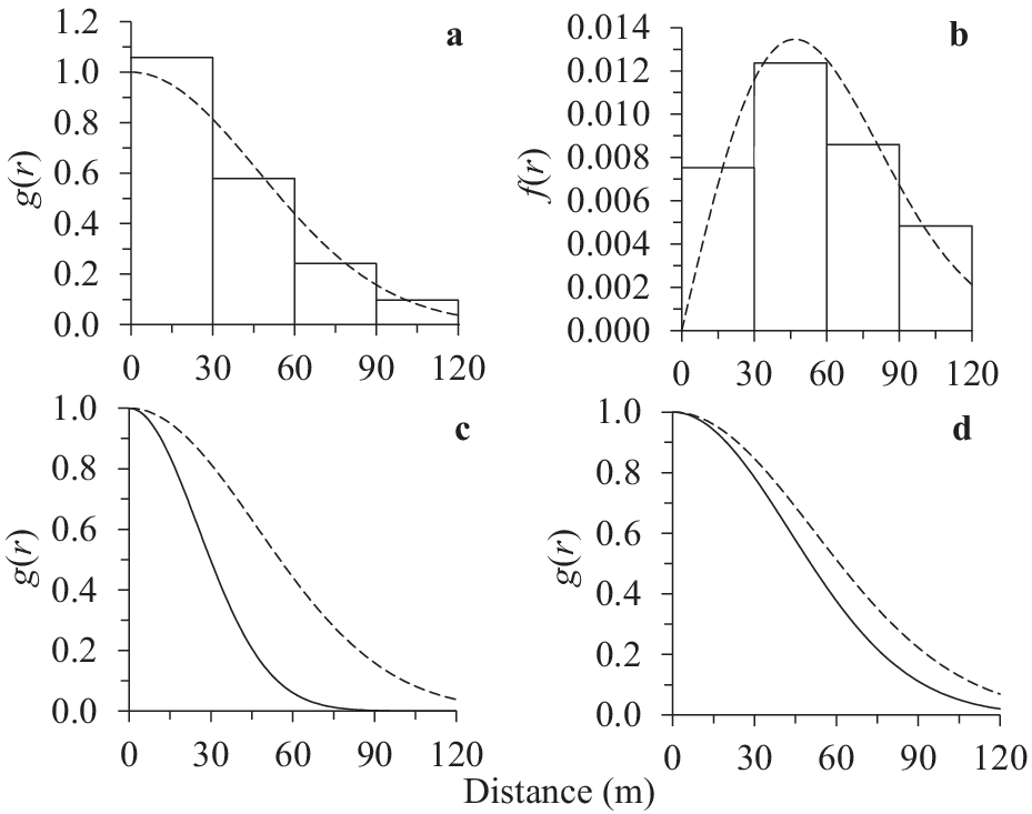
We made 65 detections (11 non-vocalising, 54 vocalising) at 41 of the 97 surveyed points. The half-normal key function without series expansion and no covariates fit the distance data (χ 2 = 2.66, df = 4, P = 0.66; AIC = 213.05, ΔAIC = 21.56; Figure 3a and b). However, the half-normal key function without series expansion and covariate detection mode had the lowest AIC (Table 1 and Figure 3c). Detection mode was the most important covariate but as we expected it did not cause extreme heterogeneity in the detection function (Table 1 and Figure 3c). Also as we expected, detectability was higher (z = 4.92, P <0.001; Figure 3c) for vocalising warblers (
 $ {\hat{P}}_d $
= 0.26, SE = 0.04) than non-vocalising warblers (
 $ {\hat{P}}_d $
= 0.04, SE = 0.02).
Barbuda Warbler (a) detection probability and (b) probability density function, based on the half-normal key function without series expansion and with covariates (c) detection mode (dashed line for vocalising, solid line for non-vocalising) and (d) Yellow Warbler (dashed line for undetected, solid line for detected) in October 2017.

Akaike information criterion values (AIC) and differences for the five top ranked multiple-covariate distance sampling half-normal models of Barbuda and Yellow Warblers in October 2017 and March 2019

a Half-normal key function. bHN without series expansion or with 1 cosine series expansion. cBarbuda Warbler (BAWA), cluster size (CLSI), detection mode (DEMO), detection time (DETI), food availability (FOAV), observer team (OBTE), point location (POLO), vegetation cover (VECO), and Yellow Warbler (YEWA). Models with ΔAIC <2 were used to estimate density. For additional information about covariates, see distance sampling in the Methods section. dNo. of parameters in the models.
The covariate Yellow Warbler was the second most important but caused less heterogeneity than detection mode (Table 1 and Figure 3c and d). As we expected, detectability of the Barbuda Warbler was higher (z = 2.20, P = 0.03; Figure 3d) at points where the Yellow Warbler was undetected (
 $ {\hat{P}}_d $
= 0.23, SE = 0.04) than detected (
 $ {\hat{P}}_d $
= 0.12, SE = 0.03). More specifically, vocalising Barbuda Warblers were more detectable (z = 3.20, P <0.001) at points where the Yellow Warbler was undetected (
 $ {\hat{P}}_d $
= 0.24, SE = 0.06) than detected (
 $ {\hat{P}}_d $
= 0.08, SE = 0.04). Vegetation cover and point location were the third and fourth most important covariates (Table 1) but caused less heterogeneity than detection mode (Figure 3c) and Yellow Warbler (Figure 3d). Contrary to what we expected, detectability did not differ between none-low and medium-high vegetation cover (z = 0.72, P = 0.47) and between points along and away from roads or tracks (z = 0.52, P = 0.60). The other covariates (i.e. CLSI, DETI, FOAV, OBTE, and TIDA) caused little heterogeneity in the detection function and contrary to what we expected had no significant effects on detectability.
The availability multiplier averaged 0.69 (SE = 0.21). Cluster size averaged 1.03 (SE = 0.02). Cluster detection was not size biased (Pearson’s correlation coefficient r = -0.10, df = 63, P = 0.44). Encounter rate n/K averaged 0.49 (SE = 0.06). Availability accounted for 69%, detectability for 17%, encounter rate for 13%, and cluster size for 1% of density variation. Density (i.e. no. of individuals/ha) averaged 0.27 (SE = 0.03) and population size (no. of individuals in the 9000-ha survey region) averaged 2,436 (SE = 261). As we expected, the Barbuda Warbler density was higher (z = 2.50, P = 0.01) at points where the Yellow Warbler was undetected (
$ \hat{D} $
= 0.23, SE = 0.03) than detected (
 $ \hat{D} $
= 0.14, SE = 0.02).
Barbuda Warbler in March 2019
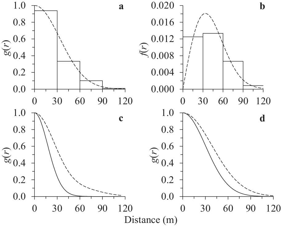
We made 160 detections (49 non-vocalising, 111 vocalising) at 57 of the 97 surveyed points. The half-normal key function with one cosine series expansion and without covariates fit the distance data (χ 2 = 2.57, df = 1, P = 0.11; AIC = 364.69, ΔAIC = 36.76; Figure 4a and b). However, the half-normal key function with one cosine series expansion and covariates detection mode, point location, and vegetation cover had the lowest AIC (Table 1). Detection mode was the most important covariate but as we expected it did not cause extreme heterogeneity in the detection function (Table 1 and Figure 4c). Also as we expected, detectability was higher (z = 3.16, P <0.001; Figure 4c) for vocalising warblers (
 $ {\hat{P}}_d $
= 0.15, SE = 0.03) than for non-vocalising warblers (
 $ {\hat{P}}_d $
= 0.05, SE = 0.01).
Barbuda Warbler (a) detection probability and (b) probability density function, based on the half-normal key function with one cosine series expansion and covariates (c) detection mode (dashed line for vocalising, solid line for non-vocalising) and (d) point location (dashed line for on road or track, solid line for off road or track) in March 2019.

The covariate point location was the second most important but caused less heterogeneity than detection mode (Table 1 and Figures 4c and d). As we expected, detectability was higher (z = 2.68, P = 0.004; Figure 4d) at points along (
 $ {\hat{P}}_d $
= 0.13, SE = 0.02) than away (
 $ {\hat{P}}_d $
= 0.07, SE = 0.01) from roads or tracks. More specifically, vocalising Barbuda Warblers were more detectable (z = 2.53, P = 0.006) along (
 $ {\hat{P}}_d $
= 0.14, SE = 0.03) than away (
 $ {\hat{P}}_d $
= 0.06, SE = 0.01) from roads or tracks. Vegetation cover and observer team were the third and fourth most important covariates (Table 1) but caused less heterogeneity than detection mode (Figure 4c) and point location (Figure 4d). Contrary to what we expected, detectability did not differ between none-low and medium-high vegetation cover (z = -1.59, P = 0.11) and between observer teams (z = 1.34, P = 0.18). The other covariates (i.e. CLSI, DETI, FOAV, OBTE, TIDA, and YEWA) caused little heterogeneity in the detection function and contrary to what we expected had no significant effects on detectability.
The availability multiplier averaged 0.74 (SE = 0.13). Cluster size averaged 1.06 (SE = 0.03). Cluster detection was not size biased (Pearson’s r = -0.12, df = 158, P = 0.13). Encounter rate averaged 1.19 (SE = 0.20). Availability accounted for 43%, detectability for 39%, encounter rate for 17%, and cluster size for 1% of density variation. Density averaged 0.40 (SE = 0.02) and population size averaged 3,570 (SE = 171). As we expected, Barbuda Warbler density was higher (z = 2.11, P = 0.02) at points where the Yellow Warbler was detected (
 $ \hat{D} $
= 0.33, SE = 0.07) than undetected (
 $ \hat{D} $
= 0.16, SE = 0.08). Also, as we expected, the density of the Barbuda Warbler increased (z = -2.60, P = 0.01) between October 2017 and March 2019.
Yellow Warbler in October 2017
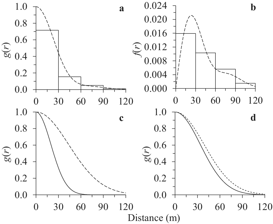
We made 44 detections (15 non-vocalising, 29 vocalising) at 30 of the 97 surveyed points. The half-normal key function without series expansion and no covariates fit the distance data (χ 2 = 8.92, df = 4, P = 0.06; AIC = 130.86, ΔAIC = 2.41; Figure 5a and b). However, the half-normal key function without series expansion and covariates detection mode and vegetation cover had the lowest AIC (Table 1). Detection mode was the most important covariate but as we expected it did not cause extreme heterogeneity in the detection function (Table 1 and Figure 5c). Also as we expected, detectability was higher (z = 2.01, P = 0.02; Figure 5c) for vocalising warblers (
 $ {\hat{P}}_d $
= 0.20, SE = 0.04) than for non-vocalising warblers (
 $ {\hat{P}}_d $
= 0.11, SE = 0.05).
Yellow Warbler (a) detection probability and (b) probability density function, based on the half-normal key function without series expansion and with covariates (c) detection mode (dashed line for vocalising, solid line for non-vocalising) and (d) vegetation cover (dashed line for none–low, solid line for medium–high) in October 2017.

The covariate vegetation cover was the second most important but caused less heterogeneity than detection mode (Table 1 and Figure 5c and d). Contrary to what we expected, detectability did not differ between none-low and medium-high vegetation cover (z = 0.59, P = 0.56; Figure 5d). The covariate observer team was the third most important (Table 1) but caused less heterogeneity than detection mode (Figure 5c) and vegetation cover (Figure 5d). Contrary to what we expected, detectability did not differ between observer teams (z = 0.60, P = 0.55). The other covariates (i.e. BAWA, CLSI, DETI, FOAV, POLO, and TIDA) caused little heterogeneity in the detection function and contrary to what we expected had no significant effects on detectability.
The availability multiplier averaged 0.68 (SE = 0.13). Cluster size averaged 1.10 (SE = 0.05). Cluster detection was not size biased (Pearson’s r = -0.37, df = 42, P = 0.16). Encounter rate averaged 0.33 (SE = 0.06). Availability accounted for 37%, detectability for 33%, encounter rate for 28%, and cluster size for 2% of density variation. Density averaged 0.68 (SE = 0.03) and population size averaged 6,093 (SE = 269).
Yellow Warbler in March 2019
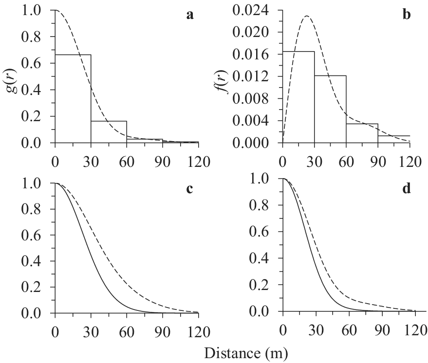
We made 218 detections (69 non-vocalising, 149 vocalising) at 58 of the 97 surveyed points. The half-normal key function with one cosine series expansion and without covariates fit the distance data (χ 2 = 8.47, df = 4, P = 0.08; AIC = 308.18, ΔAIC = 20.43; Figure 6a and b). However, the half-normal key function with one cosine series expansion and covariates detection mode, detection time, and cluster size had the lowest AIC (Table 1). Detection mode was the most important covariate but as we expected it did not cause extreme heterogeneity in the detection function (Table 1 and Figure 6c). Also as we expected, detectability was higher (z = 2.18, P = 0.03; Figure 6c) for vocalising warblers (
 $ {\hat{P}}_d $
= 0.17, SE = 0.04) than for non-vocalising warblers (
 $ {\hat{P}}_d $
= 0.08, SE = 0.01).
Yellow Warbler (a) detection probability and (b) probability density function, based on the half-normal key function with one cosine series expansion and covariates (c) detection mode (dashed line for vocalising, solid line for non-vocalising) and (d) detection time (dashed line for 0-3 minutes, solid line 4-6 minutes) in March 2019.

The covariate detection time was the second most important but caused less heterogeneity than detection mode (Table 1 and Figure 6c and d). As we expected, detectability was higher (z = 2.16, P = 0.03; Figure 6d) during the first (
 $ {\hat{P}}_d $
= 0.18, SE = 0.05) than during the last three minutes (
 $ {\hat{P}}_d $
= 0.07, SE = 0.01) of the six-minute counts. More specifically, vocalising warblers were more detectable (z = 2.23, P = 0.03) during the first (
 $ {\hat{P}}_d $
= 0.18, SE = 0.06) than during the last three minutes (
 $ {\hat{P}}_d $
= 0.06, SE = 0.02) of the counts. Cluster size and food availability were the third and fourth most important covariates (Table 1) but caused less heterogeneity than detection mode (Figure 6c) and detection time (Figure 6d). As we expected, cluster detectability was size biased (Pearson’s r = -0.24, df = 216, P <0.001). However, contrary to what we expected, detectability did not differ between none-low and medium-high food availability (z = -0.31, P = 0.76). The other covariates (i.e. BAWA, DETI, OBTE, POLO, TIDA, and VECO) caused little heterogeneity in the detection function and contrary to what we expected had no significant effects on detectability.
The availability multiplier averaged 0.72 (SE = 0.19). Expected cluster size averaged 1.11 (SE = 0.02). Encounter rate averaged 1.62 (SE = 0.24). Availability accounted for 59%, detectability for 22%, encounter rate for 16%, and cluster size for 3% of density variation. Density averaged 0.80 (SE = 0.04) and population size averaged 7,158 (SE = 358). As we expected, the density of the Yellow Warbler increased (z = -2.40, P = 0.02) between October 2017 and March 2019.
Discussion
We obtained the first distance sampling total abundance estimates for the endemic Barbuda Warbler and resident Yellow Warbler, accounting for incomplete counts due to imperfect detection at the surveyed points. Detection mode was the most important covariate. Other covariates, including point location, detection time, and cluster size, yielded inconsistent results and did not influence detectability to the same extent as detection mode in October 2017 and March 2019. Vocalising warblers were more detectable than non-vocalising warblers during the surveys. In October 2017, vocalising Barbuda Warblers were more detectable at points where the Yellow Warbler was undetected than detected. Moreover, because both detectability and density of the Barbuda Warbler were higher at points where the Yellow Warbler was undetected than detected in October 2017, we suggest competitive interactions may have occurred due to the loss of vegetation cover and food supplies following the hurricane. However, Barbuda Warbler detectability did not differ, and its density was higher at points where the Yellow Warbler was detected than undetected in March 2019. In contrast to Einarsson (Reference Einarsson2007) and Mahabir (Reference Mahabir2018), who did not account for species-specific differences in detection probability, we suggest the warblers coexisted non-competitively after population recovery from the hurricane. Despite these findings, we emphasise that distance sampling detectability and density estimates can only provide circumstantial evidence of interspecific interactions. Any observed pattern from survey-based count data, such as the negative and positive density associations between Barbuda and Yellow Warblers in October 2017 and March 2019, may be coincidental or sporadic, and likely be consistent with various non-mutually exclusive process explanations. For example, diffuse exploitative competition and coexistence due to diet, foraging behaviour, and substrate use differences among warblers show similar density responses to insect abundance fluctuations (see Sherry and Kent Reference Sherry and Kent2022).
The total abundance estimates of Barbuda and Yellow Warblers increased between October 2017 and March 2019. This finding suggests population resilience to the hurricane, likely due to high birth rates and fast recovery from lowered densities (e.g. see Pimm Reference Pimm1991; Chapter 2). However, we do not have total abundance estimates to determine if the warbler populations recovered or remained below pre-hurricane levels. All we can say with the evidence at hand is that the population size estimate for October 2017 (i.e.
 $ \hat{N} $
= 2,436, SE = 261) overlapped and the March 2019 estimate (i.e.
 $ \hat{N} $
= 3,570, SE = 171) was higher than the expert-based population range of 1,000-2,500 individuals given for the Barbuda Warbler in 2000 (Birdlife International 2024b). Although the Barbuda Warbler population seems to be larger than previously thought, its limited distribution range, combined with threats from hurricanes and habitat loss on the island, warrants the classification of Vulnerable (Birdlife International 2024b). However, the more abundant and widely distributed Yellow Warbler should continue to be classified as of Least Concern (Birdlife International 2024a).
Mahabir’s (Reference Mahabir2018) field observations and mist-netting data suggest that the Barbuda and Yellow Warblers have a peak in reproductive activity between May and June. Like other resident insectivorous birds that have adapted to arid environments on Caribbean islands, reproduction seems to be influenced by rainfall during the first half of the year (e.g. see Faaborg et al. Reference Faaborg, Arendt and Kaiser1984). For monitoring seasonal and annual changes in total abundance, we recommend training observers from local and regional partner organisations (see Acknowledgements) and conducting the surveys at least biennially in March (pre-reproduction) and October (post-reproduction). Moreover, conventional and multiple-covariate distance sampling can be extended with two-stage and hierarchical models to study the effects of environmental covariates (e.g. land-cover class, habitat type, and disturbance from development) on warbler point-level densities (see Buckland et al. Reference Buckland, Rexstad, Marques and Oedekoven2015; Chapters 7 and 8; Kéry and Royle Reference Kéry and Royle2016; Chapters 8 and 9). Conservation efforts from partner organisations should aim to maintain Barbuda Warbler total abundance above March 2019 levels (say, >0.56 individuals/ha and
 $ \hat{N} $
>5,000 individuals in the 9,000-ha survey region; see Traill et al. Reference Traill, Brook, Frankham and Bradshaw2010). More than 5,000 individuals may be needed to maintain demographic sustainability (births >deaths), ecological functionality (interspecific interactions and coexistence mechanisms), and population resilience (fast recovery time from lowered densities) in the face of increasing threats from anthropogenic and natural disturbances (Pimm Reference Pimm1991; Sanderson Reference Sanderson2006; Traill et al. Reference Traill, Brook, Frankham and Bradshaw2010).
Acknowledgements
Two anonymous reviewers provided helpful suggestions to improve the manuscript. Fieldwork was possible thanks to Birds Caribbean and the financial support of the U.S. Fish and Wildlife Service’s Neotropical Migratory Bird Conservation Act, Global Wildlife Conservation, and Mr Lamont Brown. Logistical support was provided by the Environmental Awareness Group and Department of Environment, thanks to the coordination of Ms Arika Hill, Ms Natalya Lawrence, Dr Helena Jeffery Brown, Ms Ruleta Camacho Thomas, Ms Sasha-Gay Middleton, Mr Kelly Burton, and Mr Henry Griffin. For field assistance, we thank Ms Shanna Challenger, Ms Sophia Steele, Ms Natalya Lawrence, and Mr Lenn Isidore from Flora and Fauna International and the Environmental Awareness Group, as well as Mr Rudolph Zachariah from the Department of the Environment, Mr Kelvin “Biggz” Samuel and Mr Dwayne Phillip from the Antigua Forestry Unit, and Mr Joseph “Junior” Prosper. We also thank the Barbuda Council and Barbudan people for their support during the surveys. Dr Anthony Diamond from the University of New Brunswick provided the location of the points established by Mr Kevin Mahabir. The findings and conclusions in this article are those of the authors and do not necessarily represent the views, determinations or policies of their respective organisations. The use of trade, firm or product names does not imply endorsement by any of the organisations involved in this assessment.