



1. Introduction
Semi-Markov games [Reference Jaśkiewicz15, Reference Minjárez-Sosa and Luque-Vásquez21, Reference Vega-Amaya28] are more general than discrete-time Markov games since the sojourn time of every state in semi-Markov games is random, while that in discrete-time Markov games [Reference Barron3, Reference Rosenberg26] is a constant. Because of this, there has been much research on semi-Markov games (see, for instance, [Reference Ghosh and Goswami10, Reference Jaśkiewicz15, Reference Minjárez-Sosa and Luque-Vásquez21, Reference Nowak23, Reference Vega-Amaya28]).
Most of the existing literature on two-person semi-Markov games focuses on the case of complete information, in which both players know all games’ information. However, in many real-world games, some information, such as players’ actions, reward information, and parameters of games, is private, and is known only by one player [Reference Aumann and Maschler2, Reference Gensbittel and Oliu-Barton12, Reference Mertens, Sorin and Zamir20, Reference Sorin27]; therefore, the study of games with incomplete information has attracted much attention (see, for instance, [Reference Aumann and Maschler2, Reference Mertens, Sorin and Zamir20, Reference Sorin27] for repeated games, [Reference Ashkenazi-Golan, Rainer and Solan1, Reference Gensbittel and Oliu-Barton12, Reference Neyman22, Reference Rosenberg26] for discrete-time Markov games, and [Reference Cardaliaguet5, Reference Gensbittel and Rainer11, Reference Grün13] for differential games). Two-person games with incomplete information are divided into two cases: the one side case (i.e. player 1 has private information and player 2 does not [Reference Cardaliaguet5, Reference Renault25]); and the both sides case (i.e. the two players both have private information [Reference Gensbittel and Rainer11, Reference Gensbittel and Oliu-Barton12]).
To the best of our knowledge, only Minjárez-Sosa and Luque-Vásquez [Reference Minjárez-Sosa and Luque-Vásquez21] have studied semi-Markov games with incomplete information on one side. They studied the case where the private information is the distribution of the sojourn time of states. Under the assumption that the distribution is independent of the states and actions, they constructed an asymptotically discount optimal pair of policies. However, there are many practical applications, such as Cournot oligopolies [Reference Einy, Haimanko, Moreno and Shitovitz9] and auction games [Reference Lizzeri and Persico19], where the private information is about the reward, making the model in [Reference Minjárez-Sosa and Luque-Vásquez21] unsuitable for these scenarios. Therefore, in this article we study semi-Markov games with incomplete reward information on one side under the discount criterion, where the private information of player 1, as in [Reference Mertens, Sorin and Zamir20, Reference Rosenberg26, Reference Sorin27], is the reward information. The private information in this article is different from that in [Reference Minjárez-Sosa and Luque-Vásquez21]. This is because the private information in this article is of the reward type, while the private information in [Reference Minjárez-Sosa and Luque-Vásquez21] is imposed on the distribution of sojourn times of states.
As in semi-Markov games with complete information [Reference Jaśkiewicz15, Reference Vega-Amaya28] and discrete-time Markov games with incomplete information on one side [Reference Rosenberg26], our goal is to establish the existence of the value function and optimal policies. However, the asymmetry of information prevents us from simultaneously proving the existence of the value function and optimal policies by the Shapley equation. Therefore, we first establish the existence of the value function by approximation, and prove the continuity and concavity of the value function. Then, using these properties of the value function, we verify that the value function solves the Shapley equation, and then construct an optimal policy for player 1 from the Shapley equation. However, since the Shapley equation does not provide information on an optimal policy for player 2 [Reference Rosenberg26], inspired by [Reference De Meyer6, Reference De Meyer7] on zero-sum discrete-time repeated games with incomplete information, we also introduce the dual game, and get an optimal policy for player 2 in the dual game. Then, using the optimal policy for player 2 in the dual game, we construct an optimal policy for player 2 in the primal game. Finally, we give two iterative algorithms for computing
 $\varepsilon$
-optimal policies for player 1 and player 2, respectively. The main contributions of this article are as follows:
-
(i) By giving a recursive relation for the expected reward for the semi-Markov game (Lemma 3.1), we prove that the value function is the unique solution of the Shapley equation (Theorem 3.2), which extends Proposition 6 in [Reference Rosenberg26] to the semi-Markov case. In particular, when the set K of reward types is a singleton, Theorem 3.2 is consistent with Proposition 3.1 (b) in [Reference Minjárez-Sosa and Luque-Vásquez21] for the case of finite states.
-
(ii) On the basis of the existence of the value function of the semi-Markov game (Theorem 3.1), inspired by [Reference De Meyer6, Reference De Meyer7, Reference Rosenberg26] we introduce a dual game for the semi-Markov game, and demonstrate that the value function of the dual game solves the dual Shapley equation (Proposition 5.2), which not only is an extension of Proposition 7 in [Reference Rosenberg26] but also is used to construct an optimal policy for player 2.
-
(iii) We develop two algorithms (Algorithms 1 and 2) to compute the
 $\varepsilon$
-optimal policies for player 1 and player 2, respectively, and also present the convergence of the two algorithms. It is obvious that the two algorithms developed here can be applied to the case of the corresponding discrete-time games.

This article is organized as follows. In Section 2, we introduce semi-Markov games with incomplete reward information. The existence of the value function is given in Section 3. The explicit construction of an optimal policy for player 1 is proposed in Section 4. In Section 5, we construct an optimal policy for player 2 by introducing dual games.
2. The Game Model and Preliminaries
Given a finite set E, denote by
 $|E|$
the cardinality of E and by
 $\mathscr{P}(E)$
the set of probability measures on E. The set
 $\mathscr{P}(E)$
is viewed as a subset of
 $\mathbb{R}^{|E|}$
, and for each
 $p=(p_i)_{i\in E}$
and
 $q=(q_i)_{i\in E} \in \mathbb{R}^{|E|}$
, define
 $\| p- q \| \, :\!= \, \sum_{i\in E}|p_i - q_i|$
. Hence,
 $(\mathscr{P}(E), \|{\cdot} \|)$
becomes a complete separable metric space [Reference Billingsley4]. For any
 $i\in E$
,
 $\delta_i$
denotes the Dirac measure concentrated on i. Write
 $\mathbb{R}_+ \, :\!= \, [0,\infty)$
. Finally, if X and Y are Borel spaces, denote by
 $\mathscr{B}(X)$
the Borel
 $\sigma$
-algebra of X and by
 $\mathscr{P}(X|Y)$
the family of stochastic kernels on X given Y.
The model of zero-sum semi-Markov games with incomplete reward information is
 \begin{equation} G(p)\, :\!= \, \{K, S, (A \times B), p, Q(\cdot, \cdot|i, a, b), c(k, i, a, b) \},\end{equation}
where K is the set of reward types, S is the set of states, and A and B are the sets of actions of player 1 and player 2, respectively. K, S, A, and B are assumed to be finite. The probability measure
 $p \in \mathscr{P}(K)$
is the distribution of the reward types, which is used to describe the incomplete reward information. Moreover, the transition mechanism of the semi-Markov game is defined by the semi-Markov kernel
 $Q(\cdot,\cdot|i,a,b)$
on
 $\mathbb{R}_+ \times S$
given
 $S \times A \times B$
, which satisfies that given any
 $i, j\in S$
,
 $a \in A$
, and
 $b \in B$
,
 $Q(\cdot,j|i,a,b)$
is a nondecreasing right continuous real-valued function on
 $\mathbb{R}_+$
with
 $Q(0, j|i, a, b)=0$
. Finally, c is a real-valued function on
 $K \times S \times A \times B$
representing the reward rate for player 1. Without loss of generality, assume that c is nonnegative and
 $ c^*=\max_{k,i,a,b}c(k,i,a,b)>0$
.
Remark 2.1. If K is a singleton, the model G(p) in (2.1) is consistent with that of complete-information semi-Markov games [Reference Jaśkiewicz15]. Moreover, if there exist a positive constant T and a stochastic kernel
 $P\in \mathscr{P}(S|S\times A\times B)$
such that
 $Q(t,j|i,a,b)=\textbf{1}_{[T,\infty)}(t)P(j|i,a,b)$
, then the model G(p) degrades into that of discrete-time Markov games with incomplete reward information [Reference Rosenberg26].
The rules of the game G(p) are as follows. At the beginning, one of reward types k is selected according to
 $p \in \mathscr{P}(K)$
and only player 1 is informed of this. At the initial decision epoch
 $t_0 = 0$
, the system stays at
 $i_0 \in S$
, and player 1 chooses an action
 $a_0 \in A$
according to
 $i_0$
and k, whereas player 2 chooses an action
 $b_0 \in B$
according only to
 $i_0$
. As a consequence of the actions chosen, the system remains in
 $i_0$
for time
 $t_1$
and jumps to
 $i_1$
according to
 $Q(\cdot,\cdot|i_0,a_0,b_0)$
, and player 1 continuously receives rewards with the rate
 $ c(k,i_0,a_0,b_0)$
in the time interval
 $[0,t_1]$
. The action pair
 $(a_0,b_0)$
is observed by both players. Then, at time
 $t_1$
, player 1 chooses an action
 $a_1 \in A$
on the basis of the reward type k,
 $(i_0, a_0, b_0)$
and the current state
 $i_1$
, while player 2 chooses an action
 $b_1 \in B$
on the basis of
 $(i_0, a_0, b_0)$
and
 $i_1 $
. The game evolves repeatedly in the above way.
From the above description, it can be seen that player 2 cannot observe the reward at each decision epoch. This setting is suitable for some practical applications. For example, consider the following network attack–defense problem, which has many variations, as referenced in [Reference Kouam, Hayel, Kamhoua, Deugoué and Tsemogne17].
Example 2.1. There is a network with N nodes, where each node can be in one of three states: good, normal, or bad, which are denoted as 1, 2, and 3, respectively. Moreover, the interaction occurs between a defender and an attacker. The defender has private information about his reward type, which is either
 $k_1$
(high maintenance cost type) or
 $k_2$
(high protection cost type). The attacker does not know the specific reward type of the defender, but possesses an empirical probability distribution about it. At any decision epoch, both the defender and the attacker observe the state
 $i=(x_1,\ldots,x_N)$
of the network, where
 $x_n\in \{1,2,3\}$
represents the state of node n, and independently choose their actions. Namely, the defender protects or maintains the node
 $a\in \{1,\ldots,N\}$
, whereas the attacker attacks the node
 $b\in\{1,\ldots,N\}$
in order to disrupt the network. Then, in this case, if the reward type is k, the reward rate for the defender is
 \begin{align*} c(k,i,a,b)=f(i)-g(k,i,a), \end{align*}
where f(i) is the payoff rate for the network operating in state i, and g(k,i,a) is the cost rate for maintaining node a if node a is bad; otherwise g(k,i,a) is the cost rate for protecting node a when the state of node a is good or normal.
On the one hand, the reward for the defender is not paid by the attacker, and thus it can be assumed that the attacker cannot observe the reward. On the other hand, this problem is modeled as a zero-sum game, because the attacker’s objective is to oppose the defender, i.e. to minimize the reward of the defender.
Next we introduce the measurable space
 $(\Omega,\mathscr{F})$
, which is based on Kitaev’s construction [Reference Kitaev and Rykov16]. Let
 $\Omega\, :\!= \, K \times ( S \times A \times B \times \mathbb{R}_+ )^{\infty},$
and let
 $\mathscr{F}$
be the corresponding product
 $\sigma$
-algebra. The elements of
 $\Omega$
are known as trajectories of the system. Then we define the random variables
 $\Lambda$
,
 $X_n$
,
 $A_n$
,
 $B_n$
, and
 $T_n$
 $(n=0,1,\ldots)$
on
 $(\Omega, \mathscr{F})$
as for each
 $\omega= (k, i_0, a_0, b_0, t_1, \ldots, i_n, a_n, b_n, t_{n+1}, \ldots) \in \Omega$
,
 \begin{align*} \Lambda (\omega) \, :\!= \, k, \ T_0(\omega)\, :\!= \,0, \ T_{n+1}(\omega) \, :\!= \, \sum_{m=1}^{n+1} t_m, \ X_n (\omega) \, :\!= \, i_n, \ A_n (\omega) \, :\!= \, a_n, \ B_n (\omega) \, :\!= \, b_n,\end{align*}
where
 $\Lambda$
is the reward-type variable,
 $T_n$
is the nth decision epoch variable,
 $X_n$
is the state variable, and
 $A_n$
(respectively
 $B_n$
) is the action variable of player 1 (respectively player 2) at the nth decision epoch. By
 $X_n$
and
 $T_n$
, we now introduce a continuous-time process
 $X_t$
as
 \begin{align*} &X_t(\omega)\, :\!= \,\sum_{n\geq 0}\textbf{ 1}_{[T_n(\omega),T_{n+1}(\omega))}(t)X_n(\omega)+\textbf{ 1}_{[\lim_{n\to \infty}T_n(\omega),\infty)}(t)i_\Delta, \ \ t\in\mathbb{R}_+,\, \omega\in \Omega,\end{align*}
where
 $i_\Delta \notin S$
is an isolated point. Here we have used the convention that
 $0i\, :\!= \,0$
and
 $0+i\, :\!= \,i$
for all
 $i\in S\cup\{i_\Delta\}$
and that
 $[t,t)=\emptyset$
for all
 $t\in \mathbb{R}_+\cup\{\infty\}$
. Similarly, let
 \begin{align*} &A_t(\omega)\, :\!= \,\sum_{n\geq 0}\textbf{ 1}_{[T_n(\omega),T_{n+1}(\omega))}(t)A_n(\omega)+\textbf{ 1}_{[\lim_{n\to \infty}T_n(\omega),\infty)}(t)a_\Delta, \ \ t\in\mathbb{R}_+, \, \omega\in \Omega,\\[2pt] &B_t(\omega)\, :\!= \,\sum_{n\geq 0}\textbf{ 1}_{[T_n(\omega),T_{n+1}(\omega))}(t)B_n(\omega)+\textbf{ 1}_{[\lim_{n\to \infty}T_n(\omega),\infty)}(t)b_\Delta, \ \ t\in\mathbb{R}_+, \, \omega\in \Omega,\end{align*}
with isolated points
 $a_\Delta\notin A$
and
 $b_\Delta\notin B$
. We do not intend to consider the processes
 $X_t$
,
 $A_t$
, and
 $B_t$
after the moment
 $\lim_{n\to \infty}T_n$
, so let
 $c(k,i_\Delta,a_\Delta,b_\Delta)=0$
. Moreover, we define
 \begin{equation*} Y_n\, :\!= \, (X_0,A_0,B_0,X_1,\ldots,A_{n-1},B_{n-1},X_{n}), \quad n\geq 0,\end{equation*}
and
 $H_n\, :\!= \, (S \times A \times B)^{n} \times S$
.
Next we give the definitions of the policies for the players. The asymmetry of information between player 1 and player 2 leads to the policies for player 1 depending on the reward type
 $k \in K$
but the policies for player 2 not depending on it.
Definition 2.1.
-
(a) A policy for player 1 is a sequence of stochastic kernels
$\pi = \{ \pi^{(k)}_n, k \in K, n \geq 0 \}$
, where
$\pi^{(k)}_n$
is a stochastic kernel on A given
$H_n$
, i.e.
$$ \pi^{(k)}_n ({\cdot} | h_n) \in \mathscr{P} (A)\quad \mbox{for all } h_n \in H_n. $$
-
(b) A policy for player 2 is a sequence of stochastic kernels
$ {\sigma} = \{ \sigma_n, n \geq 0 \}$
, where
$\sigma_n$
is a stochastic kernel on B given
$H_n$
.


Denote by
 $\Pi_{1}$
and
 $\Pi_2$
the sets of all policies for player 1 and player 2, respectively. Given any
 $p=(p_k)_{k\in K} \in \mathscr{P}(K)$
,
 $i \in S$
,
 $\pi=\{\pi_n^{(k)},k\in K,n\geq 0\}\in \Pi_1$
, and
 $\sigma=\{\sigma_n, n\geq 0\}\in \Pi_2$
, by Tulcea’s theorem (see [Reference Hernández-Lerma and Lasserre14, Proposition C.10]) there is a unique probability measure
 $\mathbb{P}_{p, i}^{\pi, \sigma}$
on
 $(\Omega, \mathscr{F})$
satisfying
 \begin{align} \mathbb{P}_{p, i}^{\pi,\sigma} & \big(X_0=i, \Lambda=k \big) = p_k, \\[-35pt] \nonumber \end{align}
 \begin{align} \mathbb{P}_{p, i}^{\pi,\sigma} & \big(A_n=a, B_n=b | \Lambda, Y_{n}, T_n\big) = \pi^{(\Lambda)}_n \big( a | Y_n\big) \sigma_n \big( b | Y_n\big), \\[-35pt] \nonumber \end{align}
 \begin{align} \mathbb{P}_{p, i}^{\pi,\sigma} & \big(T_{n+1} - T_n \leq t, X_{{n+1}} = j | \Lambda, Y_{n}, T_n, A_n, B_n\big) = Q\big(t, j| X_n, A_n, B_n\big). \end{align}
Consequently, (2.2)–(2.4) imply that
 \begin{equation} \mathbb{P}_{p, i}^{\pi, \sigma} = \sum_{k \in K} p_k \mathbb{P}_{\delta_k, i}^{\pi, \sigma}\quad \mbox{for all } i \in S,\, \pi \in \Pi_{1}, \, \sigma \in \Pi_{2}.\end{equation}
Here and in what follows, we denote by
 $\mathbb{E}_{p, i}^{\pi,\sigma}$
the expectation with respect to
 $\mathbb{P}_{p, i}^{\pi,\sigma}$
. Fix any discount factor
 $\alpha > 0$
. For any initial state
 $i \in S$
and policy pair
 $(\pi,\sigma) \in \Pi_{1}\times \Pi_{2}$
, the expected discount reward for player 1 in the game G(p) is defined as
 \begin{equation} V (p, i, \pi, \sigma) \, :\!= \, \mathbb{E}_{p, i}^{\pi, \sigma} \bigg[ \int_0^\infty \mathrm{e}^{-\alpha t} c \big(\Lambda, X_t, A_t, B_t\big) \mathrm{d} t \bigg].\end{equation}
Furthermore, for each
 $p\in \mathscr{P}(K)$
, define the lower and upper value functions of G(p) as
 \begin{equation*} \underline{V} (p, i) \, :\!= \, \sup\nolimits_{\pi \in \Pi_{1}} \inf_{\sigma \in \Pi_{2}} V(p, i, \pi, \sigma)\ \text{and}\ \overline{V} (p, i) \, :\!= \, \inf_{\sigma \in \Pi_{2}} \sup\nolimits_{\pi \in \Pi_{1}} V(p, i, \pi, \sigma), \quad i\in S.\end{equation*}
Given any
 $\hat{\pi}\in \Pi_{1}$
, it holds that
 $ V(p,i, \hat{\pi} ,{\sigma})\leq \sup\nolimits_{\pi\in \Pi_{1}} V(p,i, \pi ,{\sigma})$
for all
 $(p,i)\in\mathscr{P}(K)\times S$
and
 $\sigma\in \Pi_{2}$
. This implies that
 \begin{align} \inf_{\sigma\in \Pi_{2}} V(p,i, \hat{\pi} ,\sigma)\leq \inf_{\sigma\in \Pi_{2}} \sup\nolimits_{\pi\in \Pi_{1}} V(p,i, \pi , {\sigma})=\overline{V}(p,i)\quad \mbox{for all } p\in \mathscr{P}(K),\, i \in S,\, \hat{\pi}\in \Pi_{1}.\end{align}
Note that the right side of (2.7) is independent of
 $\hat{\pi}\in \Pi_{1}$
; therefore,
 \begin{align*} \underline{V}(p,i)=\sup\nolimits_{\pi\in \Pi_{1}} \inf_{\sigma\in \Pi_{2}} V(p,i, {\pi} ,\sigma)\leq \overline{V}(p,i)\quad \mbox{for all } p\in \mathscr{P}(K),\, i \in S.\end{align*}
Hence, if
 $\underline{V} \geq \overline{V} $
, it holds that
 $\underline{V} = \overline{V} $
. In this case, the common function is denoted by
 $V^*$
and is called the value function of G(p). The definition of the optimal policies is given below.
Definition 2.2. Given any
 $\varepsilon\geq 0$
, a policy
 $\pi^* \in \Pi_{1}$
is called
 $\varepsilon$
-optimal for player 1 in G(p) if
 $$\inf_{\sigma \in \Pi_{2}} V (p, i, \pi^*, \sigma ) \geq \underline{V} (p, i)-\varepsilon \quad \mbox{for all } i \in S.$$
Similarly, for any
 $\varepsilon\geq 0$
, a policy
 $\sigma^* \in \Pi_{2}$
is called
 $\varepsilon$
-optimal for player 2 in G(p) if
 $$\sup\nolimits_{\pi \in \Pi_{1}} V(p, i, \pi, \sigma^*) \leq \overline{V} (p, i)+\varepsilon \quad \mbox{for all } i \in S.$$
A 0-optimal policy for player 1 (or player 2) is called optimal.
The goal of this article is to show the existence of the value function and find optimal policies for player 1 and player 2 in G(p). At the end of this section, we propose the following useful proposition, which shows that under the finiteness of S, A, and B, players only need to make finite decisions in any bounded time interval.
Proposition 2.1.
-
(a) Let
$\delta = \min\limits_{(i,a,b)\in S\times A\times B} \delta(i,a,b)$
with
then we have
$$ \delta(i,a,b)\, :\!= \, \tfrac{1}{2}\min\big\{t\in \mathbb{R}_+: D(t|i,a,b)\geq\tfrac{1}{2} \big\},$$
$\delta>0$
and
$D(\delta|i,a,b)\leq \frac{1}{2} $
for all
$(i,a,b)\in S\times A\times B$
, where
(2.8)
\begin{equation} D (t | i, a, b) \, :\!= \, \sum_{j \in S} Q(t, j | i, a, b), \quad t\in \mathbb{R}_+, (i, a, b) \in S \times A \times B. \end{equation}
-
(b) It holds that
$\mathbb{P}_{p, i}^{\pi, \sigma}(\!\lim_{n\to \infty} T_{n} = \infty ) =1$
for all
$p \in \mathscr{P}(K)$
,
$i \in S$
, and
$(\pi, \sigma) \in \Pi_{1} \times \Pi_{2}.$


Proof. (a) For any
 $(i,a,b)\in S\times A\times B$
, since
 $Q(\cdot,j|i,a,b)$
is nondecreasing and right continuous for each
 $j\in S$
,
 $D({\cdot}|i,a,b)$
is also nondecreasing and right continuous. Therefore, by
 $\lim_{t\to \infty}D(t|i,a,b)=1$
and the finiteness of
 $S\times A\times B$
, we have that
 $\delta$
is well-defined. Moreover, noting that
 $Q(0,j|i,a,b)=0$
for all
 $j\in S$
, we obtain by (2.8) that
 $D(0|i,a,b)=0$
. Therefore, it holds that
 $D(\delta_{i,a,b}|i,a,b)\leq \frac{1}{2}$
and
 $\delta_{i,a,b}>0$
, which yields
 $\delta>0$
and
 $ D(\delta|i,a,b)\leq D( \delta_{i,a,b}|i,a,b)\leq \frac{1}{2}. $
(b) Using part (a) and (2.2)–(2.4), we show by induction that
 \begin{equation} \mathbb{E}_{p, i}^{\pi, \sigma} \big[ \mathrm{e}^{- \theta T_n} \big] \leq 2^{-n}\big(1 +\mathrm{e}^{- \theta\delta}\big)^n \quad \mbox{for all } n \geq 1,\, \theta>0. \end{equation}
So for any
 $M>0$
, we have
 $\mathbb{P}_{p, i}^{\pi, \sigma} \left( T_{n} \leq M \right) \leq \mathrm{e}^M 2^{-n}(1 +\mathrm{e}^{- \theta\delta})^n$
, which implies
 $\mathbb{P}_{p, i}^{\pi, \sigma} (\!\lim\limits_{n\to \infty} T_{n} \leq M ) = 0$
. Then the arbitrariness of M gives
 $\mathbb{P}_{p, i}^{\pi, \sigma} (\!\lim\limits_{n\to \infty} T_{n} = \infty ) =1$
. This completes the proof.
3. The Value Function
This section focuses on the value function
 $V^*$
. One of the main conclusions in this section is that for each
 $p \in \mathscr{P} (K)$
, the value function of G(p) always exists, as stated in Theorem 3.1. The other main conclusion is that the value function
 $V^*$
solves the Shapley equation; see Theorem 3.2.
To establish the existence of the value function, define the expected discount reward up to the nth decision epoch as
 \begin{align} V_n (p, i, \pi, \sigma) = {\alpha^{-1}}\sum_{m=0}^n \mathbb{E}_{p, i}^{\pi, \sigma} \big[ \! \left(\mathrm{e}^{-\alpha T_m} - \mathrm{e}^{- \alpha T_{m+1}} \right) c(\Lambda, X_m, A_m, B_m) \big].\end{align}
Denote by
 $\overline{V_n} $
and
 $\underline{V_n} $
the upper and lower value functions of
 $V_n$
, respectively, i.e.
 $$\overline{V_n} (p,i)\, :\!= \,\inf_{\sigma\in \Pi_{2}}\sup\nolimits_{\pi\in \Pi_{1}}V_n(p,i,\pi,\sigma),\quad \underline{V_n} (p,i)\, :\!= \,\sup\nolimits_{\pi\in \Pi_{1}}\inf_{\sigma\in \Pi_{2}}V_n(p,i,\pi,\sigma).$$
If
 $\overline{V_n} \equiv \underline{V_n}$
, we denote the common functions by
 $V^*_n$
. We will prove the existence of the value function
 $V^* $
of G(p) by the existence of
 $V_n^* $
.
Theorem 3.1.
-
(a) For any
$n\geq 0$
, it holds that
\begin{equation*} \overline{V_n} (p, i) = \underline{V_n} (p, i)=V_n^*(p,i)\quad \mbox{for all } (p,i)\in \mathscr{P}(K)\times S. \end{equation*}
-
(b) For any
$\varepsilon>0$
, let
$ N_\varepsilon = \min\{n\in \mathbb{N}|n>\left| \ln ({\alpha \varepsilon}/{c^*}) \right| \big/ \left| \ln \beta\right| \}$
with
(3.2)where
\begin{equation} \beta\, :\!= \, \frac{1+ \mathrm{e}^{-\alpha\delta}}{2} < 1, \end{equation}
$\delta$
is defined in Proposition 2.1(a). Then for any
$n\geq N_\varepsilon$
it holds that
\begin{equation*} V(p, i, \pi, \sigma) - V_n (p, i, \pi, \sigma) \leq \varepsilon \quad \mbox{for all } (p,i)\in \mathscr{P}(K)\times S,\, (\pi,\sigma)\in \Pi_{1}\times \Pi_{2}. \end{equation*}
-
(c) The value function
$V^*$
exists and satisfies
$$ V^* (p, i) = \lim_{n \to \infty} V_n^* (p, i)\quad \mbox{for all } (p,i)\in \mathscr{P}(K)\times S. $$





Proof. (a) Part (a) follows from the Kuhn theorem [Reference Sorin27, Theorem D.1] and the von Neumann minimax theorem [Reference Barron3, Theorem 1.2.3].
(b) Since the function c is nonnegative,
 $V_n$
is nondecreasing with respect to
 $n \geq 0$
. Moreover, the monotone convergence theorem implies that
 \begin{align*} V (p, i, \pi, \sigma) = {\alpha^{-1}} \sum_{m=0}^{\infty} \mathbb{E}_{p, i}^{\pi, \sigma} \big[ \left( \mathrm{e}^{- \alpha T_m} - \mathrm{e}^{- \alpha T_{m+1}} \right) c(\Lambda, X_m, A_m, B_m) \big]. \end{align*}
Then by Proposition 2.1 and (2.9) we have that for any
 $n\geq 0$
,
 \begin{align} V (p, i, \pi, \sigma) - V_n (p, i, \pi, \sigma) \leq \frac{c^*}{\alpha} \mathbb{E}_{p, i}^{\pi, \sigma} \big[\mathrm{e}^{-\alpha T_{n+1}}- \mathrm{e}^{-\alpha T_{\infty}}\big] \leq \frac{c^*}{\alpha}\beta^{n+1}, \end{align}
with
 $T_\infty\, :\!= \,\lim\limits_{n\to\infty}T_n$
. Therefore, for any
 $\varepsilon>0$
, it follows from the definition of
 $N_\varepsilon$
that
 $$ V (p, i, \pi, \sigma) - V_n (p, i, \pi, \sigma) \leq \frac{c^*}{\alpha}\beta^{{|\ln ({\alpha \varepsilon}/{c^*})|}/{\left|\ln \beta\right| } } \leq \varepsilon \quad \mbox{for all } n\geq N_\varepsilon.$$
(c) For each
 $n \geq 0$
,
 $p \in \mathscr{P} (K)$
, and
 $ i \in S$
, the fact that
 $V_n \leq V$
implies
 \begin{equation} \underline{V_n}(p,i)=\sup\nolimits_{\pi \in \Pi_{1}} \inf_{\sigma \in \Pi_{2}} V_n (p, i, \pi, \sigma) \leq \sup\nolimits_{\pi \in \Pi_{1}} \inf_{\sigma \in \Pi_{2}} V(p, i, \pi, \sigma)=\underline{V}(p,i). \end{equation}
On the other hand, for each
 $\varepsilon > 0$
, part (b) ensures that
 $$ \overline{V}(p, i) \leq\inf_{\sigma \in \Pi_{2}} \sup\nolimits_{\pi \in \Pi_{1}} ( V_n (p, i, \pi, \sigma)+\varepsilon) =\overline{V_n} (p, i) + \varepsilon \quad \mbox{for all } n\geq N_\varepsilon, $$
which, together with part (a) and (3.4), gives
 \begin{equation} V^*_n (p, i) \leq \underline{V}(p, i) \leq \overline{V}(p, i ) \leq V^*_n (p, i) + \varepsilon \quad \mbox{for all } n\geq N_\varepsilon. \end{equation}
Since
 $V_n^* $
is bounded and nondecreasing with respect to n, the limit
 $\lim_{n \to \infty} V_n^* (p, i)$
exists. Therefore, by (3.5) and the arbitrariness of
 $\varepsilon$
, we get part (c).
Next we prove the other main conclusion of this section, which is that the value function
 $V^*$
solves the Shapley equation. To derive the Shapley equation, we deduce the recursive relation of
 $V_n$
and V in the following result. For convenience, we introduce some concepts and notation.
-
(i) Given any
$(i,a,b)\in S\times A\times B$
, the one-step-forward policy of
$\pi=\{\pi_n^{(k)},k\in K, n\geq 0\} \in \Pi_{1}$
is denoted by
$^{(i, a, b)}\pi=\{{^{(i, a, b)}\pi}_n^{(k)},n\geq 0, k\in K\}$
, which is defined by
(3.6)The one-step-forward policy
\begin{equation} {^{(i, a, b)}\pi}_n^{(k)} ({\cdot}| h_n) \, :\!= \, \pi_{n+1}^{(k)} (\cdot | i, a, b, h_{n}), \quad h_n \in H_n. \end{equation}
$^{(i, a, b)}\sigma=\{{^{(i, a, b)}\sigma}_n, n\geq 0\}$
of
$\sigma \in \Pi_{2}$
is similarly defined.
-
(ii) For any
$\mu \in \mathscr{P}(A|K)$
and
$a \in A$
, we define a mapping
$\mathbb{G}_{\mu,a}\,:\, \mathscr{P}(K) \to \mathscr{P}(K)$
as
(3.7)
\begin{equation} \mathbb{G}_{\mu, a} (p) (k) \, :\!= \, \frac{\mu(a|k)p_k}{\sum_{l \in K} \mu(a|l)p_l}, \quad p=(p_k)_{k\in K} \in \mathscr{P} (K), \, k \in K. \end{equation}


Lemma 3.1. For any
 $n\geq 0$
, the function
 $V_n(p, i, \pi, \sigma)$
satisfies
 \begin{align} & V_{n+1} (p, i, \pi, \sigma) = \sum_{k,a ,b } p_k \pi_0^{(k)} (a | i) \sigma_0 (b | i) c (k, i, a, b) \int_0^\infty \mathrm{e}^{-\alpha t} (1 - D(t | i, a, b)) \, \mathrm{d} t \nonumber \nonumber \\[2pt] & + \sum_{k,a, b} p_k \pi_0^{(k)} (a|i) \sigma_0 (b|i) \sum_{j} \int_{\mathbb{R}_+} \mathrm{e}^{-\alpha t} V _n\big(\mathbb{G}_{\pi_0 (\cdot | i), a} (p), j, {^{(i, a, b)}\pi}, {^{(i, a, b)}\sigma}\big) Q (\mathrm{d} t, j| i, a, b), \end{align}
where
 $D(t | i, a, b)$
is defined in (2.8) and
 $\pi_0 (\! \cdot \! | i)=(\pi_0^{(k)} (\! \cdot | i),k\in K)\in \mathscr{P}(A|K)$
. Moreover, we have
 \begin{align} & V (p, i, \pi, \sigma) =\sum_{k,a ,b } p_k \pi_0^{(k)} (a | i) \sigma_0 (b | i) c (k, i, a, b) \int_0^\infty \mathrm{e}^{-\alpha t} (1 - D(t | i, a, b)) \, \mathrm{d} t \nonumber \\[2pt] & + \sum_{k,a, b} p_k \pi_0^{(k)} (a|i) \sigma_0 (b|i) \sum_{j} \int_{\mathbb{R}_+} \mathrm{e}^{-\alpha t}V \big(\mathbb{G}_{\pi_0 (\cdot | i), a} (p), j, {^{(i, a, b)}\pi}, {^{(i, a, b)}\sigma}\big) Q (\mathrm{d} t, j| i, a, b) . \end{align}
Proof. Fix any
 $n\geq 0$
. By (2.2)–(2.4) and (3.1), we have
 \begin{align} V_{n+1} (p, i, \pi, \sigma) & = \sum_{k,a, b} p_k \pi_0^{(k)} (a|i) \sigma_0 (b|i) c(k, i, a, b) \int_0^\infty \mathrm{e}^{-\alpha t} \left(1 - D (t | i, a, b)\right) \mathrm{d} t \nonumber \\[2pt] & \quad + \mathbb{E}_{p, i}^{\pi, \sigma} \left[ \sum_{m=1}^{n+1} {\alpha^{-1}} \big(\mathrm{e}^{-\alpha T_m} - \mathrm{e}^{-\alpha T_{m+1}}\big) c(\Lambda, X_m, A_m, B_m) \right]\!. \end{align}
For the second item in (3.10), we first calculate the conditional expectation as follows:
 \begin{align*} & \mathbb{E}_{p, i}^{\pi, \sigma} \Big[ \big( \mathrm{e}^{-\alpha (T_m - T_1)} - \mathrm{e}^{-\alpha (T_{m+1} - T_1)} \big) c(\Lambda, X_m, A_m, B_m) \big|\Lambda,X_0,A_0 , B_0, X_1 ,T_1 \Big] \nonumber \\[2pt] &\quad= \sum_{h_0}\!\delta_{X_1}(h_0)\sum_{a_0, b_0} \pi_1^{(\Lambda)} (a_0 | X_0,A_0,B_0,h_{0}) \sigma_1(b_0 | X_0,A_0,B_0,h_{0}) \sum_{i_1}\! \int_{\mathbb{R}_+}\! Q(\mathrm{d} t_1, i_1| i_0, a_0, b_0)\nonumber \\[2pt] &\quad \cdots \sum_{a_{m-1}, b_{m-1}} \pi_{m}^{(\Lambda)} (a_{m-1}| X_0,A_0,B_0,h_{m-1}) \sigma_{m} (b_{m-1} | X_0,A_0,B_0,h_{m-1}) \nonumber \\[2pt] &\quad \times\sum_{i_{m}} \int_{\mathbb{R}_+} Q(\mathrm{d} t_{m}, i_{m} | i_{m-1}, a_{m-1}, b_{m-1})c(\Lambda, i_{m-1}, a_{m-1}, b_{m-1})\\ &\quad \times\bigg( \mathrm{exp}\bigg({-\alpha \sum\limits_{l=1}^{m-1} t_l}\bigg) - \mathrm{exp}\bigg({-\alpha \sum\limits_{l=1}^{m} t_l}\bigg) \bigg) \nonumber \\[2pt] &\quad = \sum_{h_0} \delta_{X_1} (h_0) \sum_{a_0, b_0} {^{(X_0,A_0,B_0)} \pi_0^{(\Lambda)}} (a_0|h_0) {^{(X_0,A_0,B_0)}\sigma_0} (b_0|h_0) \sum_{i_1} \int_{\mathbb{R}_+} Q(\mathrm{d} t_1, i_1|i_0,a_0,b_0) \nonumber \\[2pt] &\quad \quad \cdots \sum_{a_{m-1}, b_{m-1}} {^{(X_0,A_0,B_0)} \pi_{m-1}^{(\Lambda)}} (a_{m-1} | h_{m-1}) {^{(X_0,A_0,B_0)}\sigma_{m-1}} (b_{m-1} | h_{m-1}) \nonumber \\[2pt] &\quad \times\sum_{i_{m}} \int_{\mathbb{R}_+} Q(\mathrm{d} t_{m}, i_{m}|i_{m-1}, a_{m-1}, b_{m-1}) c(\Lambda, i_{m-1}, a_{m-1}, b_{m-1})\\ &\quad\times\bigg(\mathrm{exp}\bigg({-\alpha\sum\limits_{l=1}^{m-1} t_l}\bigg) - \mathrm{exp}\bigg({-\alpha \sum\limits_{l=1}^{m} t_l}\bigg) \bigg) \nonumber \\[2pt] &\quad = \mathbb{E}_{\delta_\Lambda, X_1}^{^{(X_0,A_0,B_0)}\pi, ^{(X_0,A_0,B_0)}\sigma} \left[ \left( \mathrm{e}^{-\alpha T_{m-1}} - \mathrm{e}^{-\alpha T_{m}} \right) c(\Lambda, X_{m-1}, A_{m-1}, B_{m-1}) \right]. \end{align*}
Hence, the second item in (3.10) satisfies
 \begin{align} & \mathbb{E}_{p, i}^{\pi, \sigma} \bigg[ \sum_{m=1}^{n+1} {\alpha^{-1}} \left(\mathrm{e}^{-\alpha T_m} - \mathrm{e}^{-\alpha T_{m+1}} \right) c(\Lambda, X_m, A_m, B_m) \bigg] \nonumber \\[3pt] &\quad=\mathbb{E}_{p, i}^{\pi, \sigma}\big[\mathrm{e}^{-\alpha T_1}\mathbb{E}_{p, i}^{\pi, \sigma}\big[V_n(\delta_{\Lambda},X_1, {^{(X_0,A_0,B_0)}\pi},{^{(X_0,A_0,B_0)}\sigma})\big|X_0,A_0,B_0,X_1,T_1\big]\big]\nonumber\\[3pt] &\quad= \sum_{k,a, b} p_k \pi_0^{(k)} (a | i) \sigma_{0} (b | i) \sum_{j} \int_{\mathbb{R}_+} \mathrm{e}^{-\alpha t} V_n (\mathbb{G}_{\pi_0 (\cdot | i), a} (p), j, {^{(i, a, b)}\pi}, {^{(i, a, b)}\sigma})Q (\mathrm{d} t, j | i, a, b), \end{align}
where the last equality is due to the fact that for each
 $(a,b)\in A\times B$
,
 $j\in S$
, and
 $D_1\in \mathscr{B}(\mathbb{R}_+)$
,
 \begin{align*} &\mathbb{E}_{p, i}^{\pi, \sigma} \big[V_n(\delta_{\Lambda},X_1, {^{(X_0,A_0,B_0)}\pi},{^{(X_0,A_0,B_0)}\sigma})\big|X_0=i, A_0=a,B_0=b,X_1=j,T_1\in D_1\big]\\[3pt] &\quad=\sum_{k\in K}\frac{p_k\pi^{(k)}_0(a|i)\sigma_{0}(b|i)\int_{D_1}Q(\mathrm{d} t,j|i,a,b)}{\sum_{l\in K}p_l\pi^{(l)}_0(a|i)\sigma_{0}(b|i)\int_{D_1}Q(\mathrm{d} t,j|i,a,b)}V_n\big(\delta_{k},j, {^{(i,a,b)}\pi},{^{(i,a,b)}\sigma}\big)\\[3pt] &\quad= V_n \big(\mathbb{G}_{\pi_0 (\cdot | i), a} (p), j, {^{(i, a, b)}\pi}, {^{(i, a, b)}\sigma}\big). \end{align*}
Hence, we complete (3.8) using (3.10) and (3.11). Finally, the monotone convergence theorem gives (3.9) by letting
 $n \to \infty $
in (3.8).
Let
 $\mathbb{M}$
be the set of all bounded real-valued functions on
 $\mathscr{P}(K) \times S$
with the sup norm
 $||\cdot||_\infty$
. Inspired by Lemma 3.1, we define operators
 $T^{\mu, \nu} $
and T from
 $\mathbb{M}$
to
 $\mathbb{M}$
as follows: for any
 $(\mu,\nu)\in \mathscr{P}(A|K)\times \mathscr{P}(B)$
,
 $u\in \mathbb{M}$
, and
 $(p, i)\in \mathscr{P}(K) \times S$
,
 \begin{align} T^{\mu, \nu} u (p, i) \, :\!= \,& \sum_{k,a , b } p_{k} \mu (a | k) \nu (b) c (k, i, a, b) \int_0^{\infty} \mathrm{e}^{-\alpha t} (1 - D(t| i, a, b)) \, \mathrm{d} t \nonumber \\ &+ \sum_{k,a , b } p_{k} \mu (a | k) \nu (b) \sum_{j } \int_{\mathbb{R}_+} \mathrm{e}^{-\alpha t} u \big(\mathbb{G}_{\mu, a} (p), j\big)Q (\mathrm{d} t, j | i, a, b), \end{align}
 \begin{align} Tu (p, i)\, :\!= \, &\sup\nolimits_{\mu \in \mathscr{P}(A|K)} \inf_{\nu \in \mathscr{P}(B)} T^{\mu, \nu} u (p, i).\end{align}
The equation
 $u = Tu$
is called the Shapley equation corresponding to the semi-Markov game with incomplete reward information.
Theorem 3.2 The value function
 $V^*$
is the unique solution to the Shapley equation, i.e.
 \begin{equation*} V^* = T V^*, \end{equation*}
and if
 $u\in \mathbb{M}$
satisfies
 $u=Tu$
then it holds that
 $u=V^*$
.
The proof of Theorem 3.2 relies on some properties of the value function and the operator T, which are developed below. For readability, we will show these properties before proving Theorem 3.2. Firstly, we give the following proposition to explain the relationship between
 $\mathbb{P}_{p, i}^{\pi, \sigma}$
and
 $(p,\pi)$
, and show the concavity of
 $V_n^*(\cdot,i)$
and
 $V^*(\cdot,i)$
over
 $\mathscr{P} (K)$
for each fixed
 $i\in S$
.
Proposition 3.1.
-
(a) For any
$p=(p_k)_{k\in K}$
,
$q=(q_k)_{k\in K} \in \mathscr{P} (K)$
,
$\pi, \hat{\pi} \in \Pi_{1}$
, and
$\lambda\in [0,1]$
, there is a policy
$\pi^{\lambda} \in \Pi_{1}$
for player 1 satisfying
\begin{equation*} \lambda \mathbb{P}_{p, i}^{\pi, \sigma} + (1- \lambda) \mathbb{P}_{q, i}^{\hat{\pi}, \sigma} = \mathbb{P}_{\lambda p + (1- \lambda) q, i}^{\pi^{\lambda}, \sigma} \quad \mbox{for all } i \in S, \, \sigma \in \Pi_{2}. \end{equation*}
-
(b) For each
$i \in S$
and
$n \geq 0$
,
$V^*_n (\cdot, i)$
is concave on
$\mathscr{P} (K)$
. Furthermore, the value function
$V^* (\cdot, i)$
is also concave on
$\mathscr{P} (K)$
.


Proof. (a) For any
 $n\geq 0$
,
 $k \in K$
,
 $a\in A$
, and
 $h_{n}= (i_0,a_0,b_0,\ldots,i_{n-1},a_{n-1},b_{n-1},i_n )\in H_n$
, define
 $C_n \big(k, h_n, a\big)$
as
 \begin{align*} C_n \big(k, h_n, a\big) \, :\!= \, &\lambda p_k \pi_n^{(k)}\big(a|h_n\big) \displaystyle\prod_{m=0}^{n-1} \pi_{m}^{(k)} \big(a_{m} | i_0,a_0,b_0,\ldots,i_{m-1},a_{m-1},b_{m-1},i_m\big) \nonumber \\[2pt] & + (1- \lambda) q_k\hat{\pi}_n^{(k)}\big(a|h_n\big)\displaystyle\prod_{m=0}^{n-1} \hat{\pi}_{m}^{(k)} \big(a_{m} | i_0,a_0,b_0,\ldots,i_{m-1},a_{m-1},b_{m-1},i_m\big). \end{align*}
For convenience, let
 $C_{-1}(k,h_{-1},a_{-1})=\lambda p_k+(1-\lambda)q_k$
. Then it holds that for each
 $k\in K$
 \begin{equation} \sum_{a \in A} C_n (k, h_n, a) = C_{n-1} (k, h_{n-1}, a_{n-1})\quad \mbox{for all } n \geq 0,\, h_n=(h_{n-1},a_{n-1},b_{n-1},i_n)\in H_n. \end{equation}
Using
 $C_n (k, h_n, a)$
, we define
 $\pi^\lambda \, :\!= \, \{\pi_n^{\lambda, (k)}, n \geq 0, k \in K\}$
as
 \begin{align} \pi_n^{\lambda, (k)} \big(a | h_n\big)\, :\!= \, \left\{ \begin{array}{lll} \frac{ C_n (k, h_n, a) }{ C_{n-1} (k, h_{n-1}, a_{n-1})}, &\quad \hbox{$C_{n-1} (k, h_{n-1}, a_{n-1}) > 0$,} \\[6pt] | A |^{-1} & \quad \hbox{otherwise.} \end{array} \right. \end{align}
By (3.14) and (3.15), it is obvious that
 $ \pi^\lambda\in \Pi_{1}$
. Let
 \begin{equation*} E_n \, :\!= \, \{k\} \times \prod_{m=0}^n \big(\{(i_m, a_m, b_m)\}\times [0,t_{m+1}] \big)\times \big( S \times A \times B \times \mathbb{R}_+ \big)^{\infty},\quad n\geq 0, \end{equation*}
where
 $t_{m+1}\in \mathbb{R}_+$
and
 $(i_m, a_m, b_m)\in S\times A\times B$
for all
 $m\geq 0$
. Then (2.3) and (2.4) show that for each
 $i\in S$
and
 $\sigma=\{\sigma_n,n\geq 0\}\in \Pi_{2}$
 \begin{align*} &\Big( \lambda \mathbb{P}_{p, i}^{\pi, \sigma} + (1- \lambda) \mathbb{P}_{q, i}^{\hat{\pi}, \sigma} \Big) \big( E_n \big) \nonumber \\[1pt] &= \delta_{i} (i_0) \bigg[ \lambda p_k \prod_{m=0}^n \pi_{m}^{(k)}\big(a_{m}|h_{m}\big)+ (1 - \lambda) q_k \prod_{m=0}^n \hat{\pi}_{m}^{(k)} \big(a_{m}|h_{m}\big) \bigg] \nonumber \\[1pt] & \times \bigg[ \prod_{m=0}^{n-1} \sigma_{m} \big(b_m | h_m\big) Q\big( t_{m+1}, i_{m+1} |i_m, a_m, b_m\big) \bigg] \sigma_n\big(b_n | h_n\big) D(t_{n+1} | i_n, a_n, b_n) \nonumber \\[1pt] &= \delta_{i} (i_0) C_{n} \big(k, h_{n}, a_{n}\big) \bigg[ \prod_{m=0}^{n-1} \sigma_{m} \big(b_m | h_m\big) Q\big( t_{m+1}, i_{m+1} |i_m, a_m, b_m\big) \bigg] \nonumber \\[1pt] & \times \sigma_n\big(b_n | h_n\big) D\big( t_{n+1} |i_n, a_n, b_n\big), \end{align*}
where
 $h_0=i_0$
,
 $h_{m+1}=(h_m,a_m,b_m,i_{m+1})$
, and
 $D(t|i,a,b)$
is defined in (2.8). On the other hand, using (3.15), we have
 $ (\lambda p_k+(1-\lambda)q_k)\prod_{m=0}^n \pi_m^{\lambda, (k)} (a_m | h_m)=C_{n} (k, h_{n}, a_{n})$
, which implies
 \begin{align*} \mathbb{P}_{\lambda p + (1- \lambda) q,i}^{\pi^\lambda, \sigma} \big( E_n \big) &= \delta_{i}(i_0) \bigg[ \prod_{m=0}^{n-1} \sigma_{m}(b_m|h_m) Q( t_{m+1}, i_{m+1} |i_m, a_m, b_m) \bigg] \nonumber \\[1pt] &\quad \times \sigma_n(b_n | h_n) D( t_{n+1} | i_n, a_n, b_n) {C_{n} \big(k, h_{n}, a_{n}\big)} \nonumber \\[1pt] &=\Big( \lambda \mathbb{P}_{p, i}^{\pi, \sigma} + (1- \lambda) \mathbb{P}_{q, i}^{\hat{\pi}, \sigma} \Big) \big( E_n \big). \end{align*}
Therefore, the monotone class theorem gives part (a).
(b) For any
 $i\in S$
,
 $n \geq 0$
, and
 $p,q \in \mathscr{P} (K)$
, by the definition of
 $\underline{V_n}$
and Theorem 3.1 (a), for each
 $\varepsilon >0$
, there are
 $\pi_p \in \Pi_{1}$
and
 $\pi_q \in \Pi_{1}$
such that
 \begin{align*} \inf_{\sigma \in \Pi_{2}} V_n \big(p, i, \pi_p, \sigma\big) \geq V^*_n(p,i) - \varepsilon, \quad \inf_{\sigma \in \Pi_{2}} V_n \big(q, i, \pi_q, \sigma\big) \geq V^*_n(q,i) - \varepsilon. \end{align*}
For each
 $\lambda \in [0, 1]$
, part (a) implies that there is
 ${\pi^\lambda} \in \Pi_{1}$
such that
 $$ V_n \big(\lambda p + (1- \lambda) q, i, {\pi^\lambda}, \sigma\big) = \lambda V_n \big(p, i, \pi_p, \sigma\big) + (1- \lambda) V_n \big(q, i, \pi_q, \sigma\big)\quad \mbox{for all } \sigma \in \Pi_{2}. $$
Hence, we have
 \begin{align*} V^*_n (\lambda p + (1- \lambda) q, i) &\geq \inf_{\sigma \in \Pi_{2}} V_n \big(\lambda p + (1- \lambda) q, i,{\pi^\lambda}, \sigma\big) \\ & \geq \lambda {V_n^*} (p, i) + (1- \lambda) {V_n^*} (q, i) - \varepsilon. \end{align*}
By letting
 $\varepsilon \to 0$
, we have that
 $V^*_n (\cdot, i)$
is a concave function on
 $\mathscr{P} (K)$
. Furthermore, Theorem 3.1 (c) gives that
 $V^* (\cdot, i)$
is also concave.
Lemma 3.2.
-
(a) For any
$(\mu,\nu)\in \mathscr{P}(A|K)\times \mathscr{P}(B)$
,
$T^{\mu,\nu}$
is a contraction operator. -
(b) T is a contraction operator on
$\mathbb{M}$
. -
(c) Given any
$(p,i)\in \mathscr{P}(K)\times S$
,
$\nu\in \mathscr{P}(B)$
, and
$\lambda\in [0,1]$
, it holds that
\begin{align*}\!\!\!\!\!\! \lambda T^{\mu_1,\nu}V^*(\,p,i) + (1-\lambda) T^{\mu_2,\nu}V^*(\,p,i) \leq T^{\lambda \mu_1+(1-\lambda)\mu_2,\nu}V^*(\,p,i)\,\, \mbox{for all } \mu_1,\mu_2\in \mathscr{P}(A|K). \end{align*}


Proof. (a) For any
 $(p,i)\in \mathscr{P}(K)\times S$
, u, and
 $v\in \mathbb{M}$
, it holds that
 \begin{align*} \big|T^{\mu,\nu}u(p,i)-T^{\mu,\nu}v(p,i) \big|\leq \sum_{k,a , b } p_{k} \mu (a | k) \nu (b) \sum_{j } \int_{\mathbb{R}_+} \mathrm{e}^{-\alpha t} ||u-v||_{\infty}Q (\mathrm{d} t, j | i, a, b). \end{align*}
Combining (2.9) and (3.2), we obtain
 \begin{align*} \big|T^{\mu,\nu}u(p,i)-T^{\mu,\nu}v(p,i) \big| \leq \beta ||u-v||_{\infty}, \end{align*}
which implies part (a).
(b) Part (b) directly follows from part (a) and the definition of T in (3.13).
(c) Fix
 $\mu_1$
,
 $\mu_2\in \mathscr{P}(A|K)$
. Then let
 $\mu_\lambda\, :\!= \,\lambda \mu_1 +(1-\lambda)\mu_2$
and
 $M_{m}^a\, :\!= \,\sum_{k\in K} p_k \mu_m (a|k)$
for
 $m=1,2$
and
 $a\in A$
. From
 \begin{align*} & \mathbb{G}_{\mu_\lambda , a} (p) (k) = \frac{ \lambda M_1^{a}}{\lambda M_1^a +(1-\lambda) M_2^a} \mathbb{G}_{\mu_1, a} (p) (k) + \frac{(1-\lambda)M_2^a}{\lambda M_1^a+ (1-\lambda)M_2^a} \mathbb{G}_{\mu_2, a} (p) (k), \end{align*}
Proposition 3.1 (b) gives that for any
 $a\in A$
and
 $j\in S$
,
 \begin{align*} &V^* \big(\mathbb{G}_{\mu_\lambda, a} (p), j\big) \nonumber \\[2pt] &\geq \frac{\lambda M_1^a}{\lambda M_1^a+(1-\lambda)M_2^a} V^* \big(\mathbb{G}_{\mu_1, a} (p), j\big) + \frac{(1-\lambda)M_2^a}{\lambda M_1^a+(1-\lambda)M_2^a} V^* \big(\mathbb{G}_{\mu_2, a} (p) , j\big). \end{align*}
Using (3.12) and the above inequality, we get part (c) by direct calculation.
We now give the proof of Theorem 3.2, which is divided into three steps.
Proof. Step 1. First, we show that
 \begin{align*} TV^*(p,i)=\inf_{\nu\in \mathcal{P}(B)}\sup\nolimits_{\mu\in \mathcal{P}(A|K)}T^{\mu,\nu}V^*(p,i)\quad \mbox{for all } (p,i)\in \mathcal{P}(K)\times S. \end{align*}
Fix any
 $r \in \mathbb{R}$
,
 $\mu_0 \in \mathscr{P}(A|K)$
, and
 $\nu_0 \in \mathscr{P}(B)$
, and define the sets
 $D(\nu_0)$
and
 $E(\mu_0)$
as
 \begin{align*} &D(\nu_0) \, :\!= \, \big\{\mu \in \mathscr{P}(A|K)\,: \, T^{\mu, \nu_0} V^* (p, i) \geq r \big\}, \nonumber \\[2pt] &E (\mu_0) \, :\!= \, \big\{\nu \in \mathscr{P}(B)\,: \, T^{\mu_0, \nu} V^* (p, i) \leq r \big\}. \end{align*}
Firstly, the fact that
 $E (\mu_0)$
is a convex closed subset of
 $\mathscr{P}(B)$
follows from
 $ T^{\mu_0, \nu} V^* (p, i)$
being linear with respect to
 $\nu \in \mathscr{P}(B)$
and from K, A, and B being finite.
Secondly, given any
 $\{ \mu_n \}_{n \geq 0} \subseteq D (\nu_0)$
satisfying
 $\mu_n \to \mu$
as
 $n \to \infty$
, we have
 $$ \lim_{n \to \infty} \mathbb{G}_{\mu_n , a} (p) (k) = \displaystyle\frac{p_k \lim_{n \to \infty} \mu_n (a | k)}{\sum_{l \in K} p_l \lim_{n \to \infty} \mu_n (a|l)} = \mathbb{G}_{\mu, a} (p) (k). $$
On the other hand, by (2.5), we obtain
 $V(p, i, \pi, \sigma) = \sum_{k \in K} p_k V(\delta_k, i, \pi, \sigma)$
for all
 $\pi\in \Pi_{1}$
and
 $\sigma\in \Pi_{2}$
. Hence, for any
 $p,q\in \mathscr{P}(K)$
, it holds that
 $|V(p, i, \pi, \sigma)-V(q, i, \pi, \sigma)| \leq \alpha^{-1}c^*||p-q||$
, which implies that
 \begin{equation} \big|V^*(p,i)-V^*(q,i)\big|\leq \alpha^{-1}c^*||p-q||\quad \mbox{for all } p,q\in \mathscr{P}(K), \, i\in S. \end{equation}
Therefore, (3.12) shows that
 $T^{\mu, \nu_0} V^*(p, i) = \lim_{n \to \infty} T^{\mu_n, \nu_0} V^* (p, i)$
, which implies that
 $D(\nu_0)$
is closed. Furthermore, Lemma 3.2 (c) ensures the convexity of the set
 $D(\nu_0)$
.
The compactness of
 $\mathscr{P}(A|K)$
and
 $\mathscr{P}(B)$
and Theorem A.7 in [Reference Sorin27] ensure that for each
 $(p,i)\in \mathscr{P}(K)\times S$
, there exist
 $\mu[p,i]\in \mathscr{P}(A|K)$
and
 $\nu[p,i] \in \mathscr{P}(B)$
such that
 \begin{align} T V^* (p, i) = &\inf_{\nu \in \mathscr{P}(B)} T^{\mu[p,i], \nu} V^* (p, i)\nonumber\\=& \sup\nolimits_{\mu \in \mathscr{P}(A|K)} T^{\mu, \nu[p,i]} V^* (p, i)=\inf_{\nu \in \mathscr{P}(B)}\sup\nolimits_{\mu \in \mathscr{P}(A|K)} T^{\mu, \nu} V^* (p, i). \end{align}
Step 2. Next we show that
 \begin{equation} T V^* (p, i) \leq V^* (p, i)\quad \mbox{for all } (p,i)\in \mathscr{P}(K)\times S. \end{equation}
Noting that
 $\mathbb{G}_{\mu[p,i],a }(p) \in \mathscr{P}(K)$
for all
 $a \in A$
and
 $ (p,i)\in \mathscr{P}(K)\times S$
with
 $\mu[p,i]\in \mathscr{P}(A|K)$
as in (3.17), we have that for each
 $\varepsilon > 0$
, there is a policy
 ${_{(i, a)}\pi} \in \Pi_{1}$
for player 1 satisfying
 \begin{align} V^* (\mathbb{G}_{\mu[p,i], a} (p), j) \leq V(\mathbb{G}_{\mu[p,i], a} (p), j, {_{(i, a)}\pi}, \sigma) + \varepsilon \quad \mbox{for all } \sigma \in \Pi_{2},\, j\in S. \end{align}
Define a policy
 $\pi^* = \{\pi_m^{*(k)}, k \in K, \ m \geq 0 \} \in \Pi_{1}$
as
 \begin{align*} \left\{ \begin{array}{l@{\quad}l} \pi_0^{*(k)} ({\cdot}| i_0) =\mu[p,i_0]({\cdot}|k), & \hbox{$ i_0 \in S$,} \\ \pi_m^{*(k)} ({\cdot} | h_m) ={_{(i_0, a_0)}\pi}_{m-1}^{(k)} ({\cdot} | i_1,a_1,b_1, \ldots, i_{m}), & \hbox{$h_m=(i_0, a_0, b_0, \ldots, i_m)\in H_m$.} \end{array} \right. \end{align*}
Using the notation introduced in (3.6), we can verify that
 $^{(i, a, b)}\pi^*= {_{(i,a)}\pi}$
. Hence, combining (3.9) with (3.19), for any
 $\sigma=\{\sigma_n\}\in \Pi_2$
, we obtain

Hence, the arbitrariness of
 $\sigma$
and
 $\varepsilon$
gives (3.18).
Step 3. We then prove the following inequality:
 \begin{equation} V^* (p, i) \leq \inf_{\nu\in \mathscr{P}(B)}\sup\nolimits_{\mu\in \mathscr{P}(A|K)}{T}^{\mu,\nu} V^* (p, i)\quad \mbox{for all } (p,i)\in \mathscr{P}(K)\times S. \end{equation}
Fix
 $\pi=\{\pi_n^{(k)}, k\in K, n\geq 0 \}\in \Pi_{1}$
. Similar to (3.19), for any
 $\varepsilon>0$
,
 $i\in S$
, and
 $a\in A $
, there exists a policy
 ${_{(i, a)}\sigma}=\{{_{(i, a)}\sigma_n},n\geq 0\} \in \Pi_{2}$
for player 2 such that
 \begin{equation*} V^* \big(\mathbb{G}_{\pi_{0} (\cdot | i), a} (p), j\big) \geq V\big(\mathbb{G}_{\pi_0 (\cdot | i), a} (p),j , \hat{\pi}, {_{(i, a)}\sigma}\big) - \varepsilon \quad \mbox{for all } \hat{\pi} \in \Pi_{1},\,j\in S. \end{equation*}
Define a policy
 $\sigma^* = \{\sigma_m^*, m \geq 0 \} \in \Pi_{2}$
as
 $$ \left\{ \begin{array}{l@{\quad}l} \sigma_0^{*} ({\cdot}|i) = \nu[p,i]({\cdot}); & \\ \sigma_m^{*} ({\cdot} | h_m) = {_{(i_0, a_0)}\sigma_{m-1}}( {\cdot} |i_1, a_1, b_1, \ldots, i_m),\,\,\, h_m = ( i_0, a_0, b_0, \ldots, i_m)\in H_m, \end{array} \right. $$
where
 $\nu[p,i]$
is given in (3.17). The rest is similar to the proof of step 2, so the details are omitted. Combining (3.17), (3.18), and (3.20), we obtain
 $V^* = T V^*$
. Finally, by Lemma 3.2 (b) and the fact that
 $\mathbb{M}$
is a Banach space, the desired result is obtained.
Remark 3.1. From the definitions of
 $T^{\mu,\nu}$
in (3.12) and
 $\mathbb{G}_{\mu,a}(p)$
in (3.7), we see that
 $ T^{\mu, \nu} u(p, i)$
may not be linear in
 $\mu$
. Therefore, there is no general approach for solving the following corresponding max-min optimization problem:
 $$\max_{\mu\in \mathscr{P} (A|K)}\min_{\nu\in \mathscr{P}(B)}T^{\mu,\nu}u(p, i),$$
i.e. computing Tu(p,i). However, for the special case that K is a singleton,
 $T^{\mu,\nu}u(p,i)$
is bilinear in
 $(\mu,\nu)$
. Hence, in this case, Tu(p,i) can be computed by the corresponding linear programming; see [Reference Barron3, Section 2.4] for details.
Noting that
 $V^*_n$
is concave and satisfies (3.8), by the same arguments as in the proof of Theorem 3.2, we get the following corollary, which provides a method for iteratively calculating
 $V_n^* (p, i)$
.
Corollary 3.1. Let
 $V_{-1}^* \equiv 0$
. For any
 $n\geq -1$
, it holds that
 \begin{equation*} V^*_{n+1}(p,i)=TV^*_n(p,i)\quad \mbox{for all } (p,i) \in \mathscr{P}(K)\times S. \end{equation*}
4. Optimal Policies for Player 1
In this section, we construct an optimal policy and propose an iterative algorithm for
 $\varepsilon$
-optimal policies for player 1 in G(p). To do this, we give a lemma for calculating posterior distributions on K.
Lemma 4.1. For each
 $p =(p_k)_{k\in K}\in \mathscr{P}(K)$
and
 $\pi=\{\pi^{(k)}_n, k\in K, n\geq 0\}\in \Pi_{1} $
, define the posterior distributions on K at the nth decision epoch by
 ${p}^{\pi}[h_{-1},a_{-1}] \, :\!= \, p$
and
 \begin{align} {p}^{\pi}[h_{n},a_{n}] \, :\!= \, \mathbb{G}_{\pi_n(\cdot | h_n), a_n} ({p}^\pi[h_{n-1},a_{n-1}]), \quad n\geq 0,\, k\in K, \end{align}
where
 $h_{n}=(h_{n-1},a_{n-1},b_{n-1},i_n)\in H_n$
,
 $\pi_n(\cdot | h_n)=(\pi_n^{(k)}(\cdot | h_n),k\in K)\in \mathscr{P}(A|K)$
, and
 $a_n\in A$
. Then the mapping
 ${p}^{\pi}[Y_n,A_n]$
from
 $\Omega$
to
 $\mathscr{P}(K)$
satisfies
 $$ p^{\pi}[Y_{n},A_{n}] (k) =\mathbb{E}^{\pi,\sigma}_{p,i}[\textbf{1}_{\{\Lambda=k\}}|Y_{n+1},T_1,T_2-T_1,\ldots,T_{n+1}-T_{n}] \,\, \mbox{for all } n \geq 0,\, \sigma\in \Pi_{2},\, k\in K. $$
Proof. By induction, we have
 $$ p^{\pi}[h_{n},a_{n}] (k)=\frac{p_k \prod_{m=0}^n \pi_{m}^{(k)}(a_m|h_m)}{\sum_{l\in K} p_l \prod_{m=0}^n \pi_{m}^{(l)}(a_m|h_m)}. $$
Then we denote
 $$E_n\, :\!= \,\prod_{m=0}^n \big(\{\big(i_{m},a_{m},b_{m}\big)\}\times D_{m+1}\big) \times \{i_{n+1}\} \times \big(A\times B\times S\times \mathbb{R}_+\big)^\infty \quad( \text{with }D_m\in \mathscr{B}(\mathbb{R}_+)).$$
Using (2.2)–(2.4), for any
 $\sigma\in \Pi_{2}$
, we obtain
 \begin{align*} &\mathbb{E}_{p,i}^{\pi,\sigma}\big[\textbf{1}_{\{\Lambda=k\}}\textbf{ 1}_{E_n}\big]\\ &\quad =p_k\delta_i(i_0)\prod_{m=0}^{n}\bigg[\pi^{(k)}_m(a_m|h_m)\sigma_m(b_m|h_m)\int_{D_{m+1}}Q(\mathrm{d} t_{m+1},i_{m+1}|i_m,a_m,b_m) \bigg]\\ &\quad =p^{\pi}[h_{n},a_{n}] (k)\sum_{l\in K}\delta_i(i_0)p_l\prod_{m=0}^{n}\bigg[\pi^{(l)}_m(a_m|h_m)\sigma_m(b_m|h_m)\\ &\quad\quad \times\int_{D_{m+1}}Q(\mathrm{d} t_{m+1},i_{m+1}|i_m,a_m,b_m) \bigg]\\ &\quad =\mathbb{E}_{p,i}^{\pi,\sigma}\big[ p^{\pi}[Y_{n},A_{n}] (k) \textbf{ 1}_{E_n}\big], \end{align*}
which, together with the monotone class theorem, implies the desired result.
Lemma 4.1 is consistent with the intuition that the posterior distribution on K has nothing to do with the actions of player 2. The reason is that player 2 does not know the reward information. Next, the main conclusion of this section is stated as follows.
Theorem 4.1. For any
 $p\in \mathscr{P}(K)$
, there exists a policy
 $\pi^* \in \Pi_{1}$
for player 1 such that
 \begin{equation*} V\big(p, i, \pi^*, \sigma\big) \geq V^*(p,i) \quad \mbox{for all } \sigma \in \Pi_{2},\, i\in S, \end{equation*}
i.e.
 $\pi^*$
is optimal for player 1 in G(p).
Proof. Firstly, for each
 $h_0=i_0\in H_0$
and
 $h_n=(h_{n-1},a_{n-1},b_{n-1},i_n)\in H_n$
(
 $n\geq 1$
), let
 \begin{equation*} p^*\big[h_{-1},a_{-1}\big] \, :\!= \, p \ \text{and}\ {p}^*\big[h_n,a_n\big] \, :\!= \, \mathbb{G}_{\mu[p^*[h_{n-1},a_{n-1}],i_n], a_n} \big(p^*[h_{n-1},a_{n-1}] \big), \end{equation*}
where
 $\mu[p^*[h_{n-1},a_{n-1}],i_n]$
is constructed by
 $p^*[h_{n-1},a_{n-1}]$
and
 $i_n$
in (4.2). In detail, assume that
 $p^*[h_{n-1},a_{n-1}] \in \mathscr{P}(K)$
for some n. Then, for any
 $i_{n}\in S$
, according to Theorem 3.2 and (3.17), there is
 $\mu[p^*[h_{n-1},a_{n-1}],i_n]\in \mathscr{P}(A|K)$
such that
 \begin{equation} V^* \big(p^*[h_{n-1},a_{n-1}], i_n\big) = \inf_{\nu \in \mathscr{P}(B)} T^{\mu[p^*[h_{n-1},a_{n-1}],i_n], \nu} V^* \big(p^*[h_{n-1},a_{n-1}], i_n\big). \end{equation}
Then, by induction, we conclude that
 $p^*[h_{n },a_{n }] \in \mathscr{P}(K)$
for all
 $n\geq 0$
,
 $h_n\in H_n$
, and
 $a_n\in A$
. Moreover, we define
 \begin{equation} \pi_n^{*(k)} \big (\cdot | h_n\big) \, :\!= \, \mu\big[p^*[h_{n-1},a_{n-1}], i_n \big](\cdot|k), \quad h_n=\big(h_{n-1},a_{n-1},b_{n-1},i_n\big)\in H_n, \end{equation}
and
 $\pi^* \, :\!= \, \{\pi^{*(k)}_n, k\in K, n\geq 0\}$
. Hence, by
 $p^*[h_{-1},a_{-1}]=p^{\pi^*}[h_{-1},a_{-1}]=p$
, we have
 \begin{equation} p^*\big[Y_n,A_n\big]=\mathbb{G}_{\pi_n^*(\cdot|Y_n), A_n} \big(p^*[Y_{n-1},A_{n-1}] \big)=p^{\pi^*}\big[Y_n,A_n\big]\quad \mbox{for all } n\geq 0. \end{equation}
Next we claim that for all
 $n \geq 0$
it holds that
 \begin{align} V^* (p, i) & \leq V_n\big(p,i,\pi^*,\sigma\big) + \mathbb{E}_{p, i}^{\pi^*, \sigma} \big[ \mathrm{e}^{-\alpha T_{n+1}} V^* (p^*[Y_n,A_n], X_{n+1}) \big] \quad \mbox{for all } i\in S,\, \sigma\in \Pi_{2}. \end{align}
This claim will be proved by induction. According to (3.12), (4.3), and (4.4), we have that (4.5) holds for
 $n=0$
. Moreover, by Lemma 4.1 and (4.2)–(4.4), for any
 $i\in S$
and
 $\sigma=\{\sigma_n,n\geq 0\}\in \Pi_{2}$
, we obtain

Hence, if (4.5) holds for
 $n-1$
, the above formula ensures that (4.5) holds for n. Letting
 $n \to \infty$
in (4.5) and using (2.9), we have
 $V^* (p, i) \leq V (p, i, \pi^*, \sigma)$
. Finally, by the arbitrariness of
 $\sigma \in \Pi_{2}$
and
 $i \in S$
, we conclude that
 $\pi^*$
is optimal for player 1 in G(p).
The proof of Theorem 4.1 gives an iterative construction of an optimal policy for player 1. However, this construction requires the value function
 $V^*$
, which is often unknown in practical applications. Intuitively, we can replace
 $V^*$
with
 $V_n^*$
, which is obtained by Corollary 3.1, to get
 $\varepsilon$
-optimal policies. Next we propose the following algorithm, by which
 $\varepsilon$
-optimal policies can be obtained within finite iterations, and prove its effectiveness.
At the end of this section, we present a proposition to show that
 $\pi^\varepsilon $
defined in (4.8) is indeed
 $\varepsilon$
-optimal for player 1.
Proposition 4.1. The policy
 $\pi^\varepsilon$
output by Algorithm 1 is
 $\varepsilon$
-optimal for player 1 in G(p).
 $\varepsilon$
-optimal policies for player 1)

Algorithm 1 Long description
An equation describing a process for computing epsilon-optimal policies in a game theory context. The equation starts with the input of the game parameters and the error epsilon greater than 0. It then outlines a series of steps to compute the value function and optimal policies for players 1 and 2. The steps involve defining probabilities, computing value functions, and updating policies iteratively until the error condition is met. The output is the policy for player 1.
Proof. Since
 $p^\varepsilon[h_{-1},a_{-1}]=p=p^{\pi^\varepsilon}[h_{-1},a_{-1}]$
, combining (4.1), (4.7), and (4.8) we conclude that
 \begin{align} p^\varepsilon[h_{n},a_{n}]= p^{\pi^\varepsilon}[h_{n},a_{n}]\quad \mbox{for all } n= 0,1,\ldots,N_{\varepsilon}-1,\, h_n\in H_n, \, a_{n}\in A. \end{align}
Next we claim that for each
 $n=0,1,\ldots,N_{\varepsilon}+1$
,
 $i\in S$
, and
 $\sigma\in \Pi_2$
it holds that
 \begin{align} V_{N_{\varepsilon}}(p,i,\pi^{\varepsilon},\sigma)- V_{ n-1}(p,i,\pi^{\varepsilon},\sigma) \geq\mathbb{E}^{\pi^{\varepsilon},\sigma}_{p,i}\big[\mathrm{e}^{-\alpha T_n}V_{N_{\varepsilon}-n}^*(p^{ {\varepsilon}}[Y_{n-1},A_{n-1}],X_n)\big], \end{align}
where
 $V_{-1}(p,i,\pi^\varepsilon,\sigma)\, :\!= \,0$
and
 $p^{ {\varepsilon}}[Y_{- 1},A_{ -1}]\, :\!= \,p$
. Fix any
 $i\in S$
and
 $\sigma=\{\sigma_n,n\geq 0\}\in \Pi_2$
. The proof of (4.10) proceeds by backward induction on n. Observe that (4.10) trivially holds for
 $n=N_{\varepsilon}+1$
due to
 $V^*_{-1}\equiv 0$
. Assume that (4.10) holds for some
 $n\in \{1,\ldots,N_{\varepsilon}+1\}$
. Then, by (3.1) and the induction hypothesis, we obtain
 \begin{align*} &V_{N_{\varepsilon}}(p,i,\pi^{\varepsilon},\sigma)- V_{ n-2}(p,i,\pi^{\varepsilon},\sigma) \nonumber \\& \quad\geq \mathbb{E}^{\pi^{\varepsilon},\sigma}_{p,i}\Big[\mathrm{e}^{-\alpha T_{n-1}}\mathbb{E}^{\pi^{\varepsilon},\sigma}_{p,i}\Big[\Big( {\alpha}^{-1}(1-\mathrm{e}^{-\alpha (T_{n}-T_{n-1})})c(\Lambda,X_{n-1},A_{n-1},B_{n-1}) \nonumber \\ &\qquad\qquad\qquad\quad+\mathrm{e}^{-\alpha (T_{n}-T_{n-1})}V_{N_{\varepsilon}-n}^*(p^{ {\varepsilon}}[Y_{n-1},A_{n-1}],X_n) \Big)\Big|Y_{n-1},T_{n-1}\Big]\Big]. \end{align*}
For any
 $h_{n-1}=(h_{n-2},a_{n-1},b_{n-1},i_{n-1})\in H_{n-1}$
and
 $t\in \mathbb{R}_+$
, we have
 \begin{align*} &\mathbb{E}^{\pi^{\varepsilon},\sigma}_{p,i}\big[ {\alpha}^{-1}(1-\mathrm{e}^{-\alpha (T_{n}-T_{n-1})})c(\Lambda,X_{n-1},A_{n-1},B_{n-1}) \nonumber \\ &\qquad\qquad\qquad\quad +\mathrm{e}^{-\alpha (T_{n}-T_{n-1})}V_{N_{\varepsilon}-n}^*(p^{ {\varepsilon}}[Y_{n-1},A_{n-1}],X_n) |Y_{n-1}=h_{n-1},T_{n-1}=t\big] \nonumber \\ &\quad=\sum_{k,a,b }p^{\pi^\varepsilon}[h_{n-2},a_{n-2}](k) \pi^{\varepsilon(k)}_{n-1}(a|h_{n-1})\sigma_{n-1}(b|h_{n-1})\Big(c(k,i_{n-1},a,b)\nonumber \\ &\quad\times \int_0^\infty \mathrm{e}^{-\alpha s}(1-D(s|i_{n-1},a,b))\mathrm{d}s +\sum_{j\in S}\int_{\mathbb{R}_+}\mathrm{e}^{-\alpha s}V_{N_{\varepsilon}-n}^*( p^{ {\varepsilon}}[h_{n-1},a] ,j)Q(\mathrm{d} s,j|i_{n-1},a,b) \Big) \nonumber \\ & \quad=T^{\mu[ {p^\varepsilon}[h_{n-2},a_{n-2}],i_{n-1}],\sigma_{n-1}(\cdot|h_{n-1})}V_{N_{\varepsilon}-n}^*( {p^\varepsilon}[h_{n-2},a_{n-2}] ,i_{n-1})\nonumber \\ & \quad\geq \inf_{\nu\in \mathscr{P}(B)}T^{\mu[ {p^\varepsilon}[h_{n-2},a_{n-2}],i_{n-1}],\nu}V_{N_{\varepsilon}-n}^*( {p^\varepsilon}[h_{n-2},a_{n-2}] ,i_{n-1}) \nonumber \\ & \quad=V_{N_{\varepsilon}-n+1}^*( {p^\varepsilon}[h_{n-2},a_{n-2}] ,i_{n-1}), \end{align*}
where the first, second, and last equalities are due to Lemma 4.1, (4.9), and (4.6), respectively. Hence, it holds that
 \begin{align*} &V_{N_{\varepsilon}}(p,i,\pi^{\varepsilon},\sigma)- V_{ n-2}(p,i,\pi^{\varepsilon},\sigma) \nonumber\\ &\quad\geq \mathbb{E}^{\pi^{\varepsilon},\sigma}_{p,i}\big[\mathrm{e}^{-\alpha T_{n-1}}\mathbb{E}^{\pi^{\varepsilon},\sigma}_{p,i}\big[V_{N_{\varepsilon}-n+1}^*( {p^\varepsilon}[Y_{n-2},A_{n-2}] ,X_{n-1})|Y_{n-1},T_{n-1}\big]\big] \nonumber\\ &\quad=\mathbb{E}^{\pi^{\varepsilon},\sigma}_{p,i}\big[\mathrm{e}^{-\alpha T_{n-1}} V_{N_{\varepsilon}-n+1}^*( {p^\varepsilon}[Y_{n-2},A_{n-2}] ,X_{n-1}) \big]. \end{align*}
Therefore, we conclude that (4.10) holds for all
 $n=0,1,\ldots,N_{\varepsilon}+1$
,
 $i\in S$
, and
 $\sigma\in \Pi_2$
. In particular, it holds that
 $$ V_{N_{\varepsilon}}(p,i,\pi^{\varepsilon},\sigma)\geq \mathbb{E}^{\pi^{\varepsilon},\sigma}_{p,i}\big[ V_{N_{\varepsilon} }^*( {p^\varepsilon}[Y_{-1},A_{-1}] ,X_{0}) \big]=V_{N_{\varepsilon} }^*( p ,i)\quad \mbox{for all } i\in S,\, \sigma\in \Pi_{2}. $$
Finally, it follows from Theorem 3.1 (b) and (3.5) that
 $$ V(p,i,\pi^\varepsilon, \sigma)\geq V_{N_{\varepsilon} }^*( p ,i) \geq V^*(p,i)-\varepsilon \quad \mbox{for all } i\in S,\, \sigma\in \Pi_{2}, $$
which together with Definition 2.2 implies the desired result.
5. Optimal Policies for Player 2
The goal of this section is to establish the existence of an optimal policy for player 2 in the game G(p). From the proof of Theorem 4.1, a natural idea is to construct an optimal policy
 $\sigma^*=\{\sigma^*_n,n\geq 0\}$
for player 2 by using Theorem 3.2. To do this, we should compute
 \begin{align} \sigma_n^*({\cdot}|h_n)=\mathrm{argmin}_{\nu\in \mathscr{P}(B)}\Big\{\max_{\mu\in \mathscr{P}(A|K)}T^{\mu,\nu}V^*\Big(\mathbb{G}_{\pi_{n-1}^*(\cdot|h_{n-1}), a_{n-1} }(p),i_n\Big)\Big\},\end{align}
with the optimal policy
 $\pi^*=\{\pi^{*(k)}_n,k\in K, n\geq 0\}$
as in Theorem 4.1. This implies that
 $\sigma^*$
may rely on the policy
 $\pi^*$
for player 1, which contradicts Definition 2.2. Therefore, we cannot ensure that
 $\sigma^*$
constructed via (5.1) is optimal, and we need to find alternative methods to achieve this goal.
Note that an auxiliary dual game was introduced by De Meyer [Reference De Meyer6, Reference De Meyer7] for computing optimal policies for player 2 in repeated games. Since then, the concept of the dual game has been widely extended to games of various types to establish the existence of optimal policies for players; for instance, see [Reference Rosenberg26] for discrete-time Markov games, [Reference De Meyer and Marino8, Reference Gensbittel and Oliu-Barton12] for repeated games with incomplete information on both sides, and [Reference Laraki18] for differential games. Inspired by the arguments in [Reference De Meyer6, Reference De Meyer7, Reference Rosenberg26], we introduce a dual game for the semi-Markov game, and then construct an optimal policy for player 2 in the primal game G(p) by the optimal policy in the dual game.
Firstly, we introduce a dual game for the semi-Markov game with incomplete reward information, which is defined as follows:
 $$G^{\#}(z)\, :\!= \, \{K, S, A \times B, z, Q(\cdot,{\cdot} |i, a, b), c(k, i, a, b) \},$$
where K, S,
 $A\times B$
, Q, and c are the same as in the primal game G(p) in (2.1). The difference is that
 $p \in \mathscr{P}(K)$
in G(p) is replaced by the real-valued vector
 $z = (z_k)_{ k \in K}\in \mathbb{R}^{|K|}$
, which is used to modify the reward; see (5.2).
The dual game
 $G^{\#}(z)$
evolves as follows: At the initial decision epoch, the system stays at
 $i_0$
and player 1 chooses a reward type
 $k \in K$
and an action
 $a_0$
according to the initial state
 $i_0$
. The reward type will not change in the subsequent evolution, but is hidden from player 2. In the meantime, player 2 chooses
 $b_0 $
on the basis of the current state
 $i_0$
. The subsequent evolution of the dual game is the same as that of the primal game.
The policy for player 2 in the dual game is coincident with that in the primal game; see Definition 2.1 (b). Nevertheless, the policy for player 1 in
 $G^{\#} (z)$
is different.
Definition 5.1. A policy
 $\pi^{\#}$
for player 1 in the dual game
 $G^{\#} (z)$
is given by two-tuples
 $(\rho, \pi)$
, where
 $\rho\in \mathscr{P}(K|S)$
and
 $\pi \in \Pi_{1}$
. Denote by
 $\Pi^{\#}_1$
the set of all policies for player 1 in the dual game
 $G^{\#} (z)$
.
For each
 $i \in S$
,
 $\pi^{\#} =(\rho,\pi) \in \Pi^{\#}_{1}$
, and
 $\sigma \in \Pi_{2}$
, Tulcea’s theorem [Reference Hernández-Lerma and Lasserre14, Proposition C.10] implies that there exists a unique probability measure
 $\mathbb{P}_{i}^{\pi^{\#}, \sigma}$
on
 $(\Omega, \mathscr{F})$
satisfying
 \begin{equation*} \mathbb{P}_{i}^{\pi^{\#}, \sigma} (E) = \mathbb{P}_{\rho(\cdot|i), i}^{\pi, \sigma} (E), \quad E \in \mathscr{F}. \end{equation*}
Denote by
 $\mathbb{E}_{i}^{\pi^{\#}, \sigma}$
the expectation corresponding to
 $\mathbb{P}_{i}^{\pi^{\#}, \sigma}$
.
Following the definition of a Fenchel conjugate of a function [Reference De Meyer7, p. 238] and considering the discounting case, we introduce the expected discount reward criterion in
 $G^{\#} (z)$
as follows: for each
 $i\in S$
,
 $\pi^{\#} =(\rho,\pi)\in \Pi^{\#}_{1}$
, and
 $\sigma \in \Pi_{2}$
,
 \begin{align} U (z, i, \pi^{\#}, \sigma) \, :\!= \, &\mathbb{E}_i^{\pi^{\#}, \sigma} \bigg[ \int_0^{{\infty}} \mathrm{e}^{-\alpha t} \big( c(\Lambda, X_t, A_t, B_t) - z(\Lambda) \big) \mathrm{d} t \bigg], \end{align}
where
 $\Lambda, X_t, A_t$
, and
 $B_t$
are the same as in (2.6). It is a routine exercise to verify that
 \begin{align*} U (z, i, \pi^{\#}, \sigma) = V(\rho(\! \cdot \! |i), i, \pi, \sigma) - {\alpha^{-1}} \langle \rho(\! \cdot \! |i), z \rangle, \end{align*}
where
 $\langle z, \rho(\! \cdot \! |i) \rangle \, :\!= \, \sum_{k \in K} z_k \rho(k|i)$
.
Similar to the primal game G(p), define
 \begin{align*} \underline{U} (z, i) \, :\!= \, \sup\nolimits_{\pi^{\#} \in \Pi^{\#}_{1}} \inf_{\sigma \in \Pi_{2}} U (z, i, \pi^{\#}, \sigma) \ \text{and} \ \overline{U} (z, i) \, :\!= \, \inf_{\sigma \in \Pi_{2}} \sup\nolimits_{\pi^{\#} \in \Pi^{\#}_{1}} U (z, i, \pi^{\#}, \sigma) . \end{align*}
If
 $\underline{U}= \overline{U}$
, the common function is called the value function of
 $G^{\#}(z)$
and is denoted by
 $U^*$
. Since we focus on optimal policies for player 2, we define only the
 $\varepsilon$
-optimal policy for player 2 in
 $G^{\#} (z)$
.
Definition 5.2. Given any
 $\varepsilon\geq0$
, a policy
 $\sigma^* \in \Pi_{2}$
is called
 $\varepsilon$
-optimal for player 2 in
 $G^{\#} (z)$
if it satisfies
 $$ \sup\nolimits_{\pi^{\#} \in \Pi^{\#}_{1}} U(z, i, \pi^{\#}, \sigma^*) \leq \overline{U} (z, i)+\varepsilon \quad \mbox{for all } i\in S. $$
Moreover, a policy
 $\sigma^* \in \Pi_{2}$
is called optimal if it is 0-optimal.
To find an optimal policy for player 2, we need the continuity and convexity of
 $\underline{U}$
or
 $\overline{U}$
, which are stated in the following lemma.
Lemma 5.1.
-
(a) For each
$i \in S$
,
$\overline{U} (\cdot, i)$
is convex on
$\mathbb{R}^{|K|}$
. -
(b) For each
$i \in S$
,
$\underline{U} (z, i)$
and
$\overline{U} (z, i)$
are continuous in z.


Proof. The proofs of parts (a) and (b) are similar to those of Proposition 3.1 and (3.16), so we omit them.
The next proposition concerns the relationship between the functions
 $\overline{V}(\underline{V})$
and
 $\overline{U}(\underline{U})$
, which ensures the existence of the value function
 $U^*$
of the dual game. The proof of this proposition is similar to the corresponding proof of Theorem 2.9 in [Reference Sorin27].
Proposition 5.1. For each
 $i \in S$
, we have
 \begin{align*} \underline{U} (z, i) = \max_{p \in \mathscr{P} (K)} \big\{ \underline{V} (p, i) - {\alpha^{-1}} \langle p, z \rangle \big\} \quad for\,all\, z \in \mathbb{R}^{|K|}, \\ \overline{U} (z, i) = \max_{p \in \mathscr{P} (K)} \big\{ \overline{V} (p, i) - {\alpha^{-1}} \langle p, z \rangle \big\} \quad for\,all\, z \in \mathbb{R}^{|K|}. \end{align*}
In the dual case, the lower and upper value functions of the primal game G(p) satisfy
 \begin{align} \underline{V} (p, i) = \min_{z \in \mathbb{B}} \big\{ \underline{U} (z, i) + {\alpha^{-1}} \langle p, z \rangle \big\} \quad for\, all \, p \in \mathscr{P} (K), \end{align}
 \begin{align} \overline{V} (p, i) = \min_{z \in \mathbb{B}} \big\{ \overline{U} (p, i) + {\alpha^{-1}} \langle p, z \rangle \big\} \quad for\, all\, p\in \mathscr{P} (K), \end{align}
where
 $\mathbb{B} \, :\!= \, \{ z\in\mathbb{R}^{|K|} | 0\leq z \leq c^*=\max_{k,i,a,b}c(k,i,a,b) \}$
is a compact subset of
 $\mathbb{R}^{|K|}$
.
It is worth noting that in both (5.3) and (5.4), the minimum points can be taken from the set
 $\mathbb{B}$
; therefore, we restrict the domain of
 $U^*$
to the set
 $\mathbb{B}\times S$
. As a direct conclusion of Theorem 3.1 (c) and Proposition 5.1, we obtain the existence of the value function in the dual game
 $G^{\#} (z)$
.
Corollary 5.1. For any
 $z\in \mathbb{B}$
, the value function of the dual game
 $G^{\#} (z)$
exists and satisfies
 \begin{equation} U^* (z, i) = \max_{p \in \mathscr{P} (K)} \big\{V^* (p, i) - {\alpha^{-1}} \langle p, z \rangle \big\} \quad \mbox{for all } i\in S. \end{equation}
Next we construct an optimal policy for player 2 in the dual game, which will be used to establish the existence of an optimal policy for player 2 in the primal game. For convenience, we first introduce some notation.
-
(i) Let
$\mathcal{M}$
denote the set of all continuous functions defined on
$\mathbb{B}\times S$
. Then it follows from Proposition 5.1 and Corollary 5.1 that
$U^*\in \mathcal{M}$
. -
(ii) A set of
$\mathbb{R}^{|K|}$
-valued bounded functions is given as
Since S and A are finite,
$$ \mathscr{L} \, :\!= \, \big\{f\,:\, A\times S \to \mathbb{R}^{|K|} \ \big| \ 0 \leq f_k (a,j) \leq c^* \quad \mbox{for all } (a,j) \in A\times S,\, k \in K \big\}. $$
$\mathscr{L}$
is compact.
-
(iii) Given any
$\mu \in \mathscr{P}(A|K)$
,
$\nu \in \mathscr{P}(B)$
, and
$u\in \mathcal{M}$
, we define a function
$\Gamma^{\mu, \nu} u \,:\, \mathscr{P} (K) \times \mathscr{L} \times \mathbb{B} \times S \to \mathbb{R}$
by
(5.6)Moreover, since u is continuous on
\begin{align} &(\Gamma^{\mu, \nu} u) (p, f, z, i) \nonumber\\ &= \sum_{k,a, b} p_k \mu (a | k) \nu (b) c (k, i, a, b) \int_0^\infty \mathrm{e}^{-\alpha t} \left( 1- D(t | i, a, b) \right) \mathrm{d} t -\frac{1}{\alpha} \langle p, z \rangle\nonumber \\ & + \sum_{k,a, b} p_k \mu (a | k) \nu (b)\sum_{j } \int_{\mathbb{R}_+} \mathrm{e}^{-\alpha t} \big( u(f(a,j), j) + \frac{1}{\alpha} \langle \mathbb{G}_{\mu , a} (p), f(a,j) \rangle \big)Q (\mathrm{d} t, j | i, a, b),\nonumber\\ &\qquad \qquad\qquad\qquad \qquad \qquad\qquad\qquad (p,f,z,i)\in \mathscr{P} (K) \times \mathscr{L} \times \mathbb{B} \times S. \end{align}
$\mathbb{B}\times S$
, it holds that
$ (\Gamma^{\cdot, \cdot} u) (\cdot, \cdot, z, i)$
is jointly continuous on
$\mathscr{P}(A|K)\times \mathscr{P}(B)\times \mathscr{P}(K)\times \mathscr{L}$
for all
$z\in \mathbb{B}$
and
$i\in S$
. Thus, by the compactness of
$\mathscr{P}(A|K)$
,
$\mathscr{P}(B)$
,
$\mathscr{P}(K)$
, and
$ \mathscr{L}$
, we can define an operator on
$\mathcal{M}$
as
(5.7)
\begin{align} \Gamma^* u (z, i) \, :\!= \, \min_{\nu \in \mathscr{P}(B)} \min_{f \in \mathscr{L}} \max_{p \in \mathscr{P}(K)} \max_{\mu \in \mathscr{P}(A|K)} (\Gamma^{\mu, \nu} u) (p, f, z, i), \ u\in \mathcal{M}, (z,i)\in \mathbb{B}\times S. \end{align}


The equation
 $u=\Gamma^*u$
is called the dual Shapley equation.
Proposition 5.2. The value function
 $U^*$
satisfies the dual Shapley equation, i.e.
 \begin{equation*} U^* (z, i) = \Gamma^* U^* ( z, i)\quad \mbox{for all } (z,i)\in \mathbb{B}\times S. \end{equation*}
Proof. Fix any
 $(z,i)\in \mathbb{B}\times S$
. Then for any
 $\phi\in \mathscr{P}(K\times A)$
and
 $\nu\in \mathscr{P}(B)$
, we define
 \begin{align} & \mathbb{H} (\phi, \nu) \, :\!= \, \sum_{k,a, b} \phi(k,a) \nu (b) c (k, i, a, b) \left( \int_0^\infty \mathrm{e}^{-\alpha t} \left( 1- D(t | i, a, b) \right) \mathrm{d}t \right) \nonumber\\ + & \sum_{k,a, b} \phi(k,a) \nu (b ) \sum_{j } \int_{\mathbb{R}_+} \mathrm{e}^{-\alpha t}V^* (\phi^a, j) Q (\mathrm{d} t, j | i, a, b) -{\alpha^{-1}}\sum_{k,a}\phi(k,a)z_k , \end{align}
where
 $\phi^a\in \mathscr{P}(K)$
is the conditional probability on K given
 $a\in A$
, i.e.
 $$\phi^a(k)=\frac{\phi(k,a)}{\sum_{l\in K}\phi (l,a)}.$$
Then, according to Theorem 3.2 and Corollary 5.1, we have
 \begin{align*} U^*(z,i) = \sup\nolimits_{\phi \in \mathscr{P}(K\times A)}\inf_{\nu \in \mathscr{P}(B)} \mathbb{H} (\phi, \nu). \end{align*}
For any
 $\lambda \in [0,1]$
and
 $\phi_1, \phi_2 \in \mathscr{P}(K\times A)$
, denote
 $\phi_\lambda=\lambda\phi_1+(1-\lambda)\phi_2$
. Noting that
 \begin{align*} \phi^a_\lambda =&\frac{\lambda \sum_{k\in K}\phi_1(k,a) }{ \sum_{k\in K}[\lambda\phi_1(k,a)+(1-\lambda)\phi_2(k,a)]} \phi_1^a\\ &+\frac{(1-\lambda) \sum_{k\in K}\phi_2(k,a) }{ \sum_{k\in K}[\lambda\phi_1(k,a)+(1-\lambda)\phi_2(k,a)]} \phi_2^a \quad \mbox{for all } a\in A \end{align*}
and by Proposition 3.1 (b), we have that the set
 $\hat{D} (\nu_0) \, :\!= \, \{ \phi \in \mathscr{P}(K\times A) : \mathbb{H} (\phi, \nu_0) \geq r\}$
is convex for all
 $\nu_0\in \mathscr{P}(B)$
and
 $r\in \mathbb{R}$
. Moreover, the definition of
 $\phi^a$
and (3.16) give that
 $\hat{D}(\nu_0)$
is closed. On the other hand, it follows from (5.8) that
 $\mathbb{H}(\phi,\nu)$
is linear in
 $\nu$
, which implies that
 $\hat{E} (\phi_0) \, :\!= \, \{\nu \in \mathscr{P}(B) : \mathbb{H} (\phi_0, \nu) \leq r \}$
is convex and closed for any
 $\phi_0 \in \mathscr{P}(K\times A)$
and
 $r\in \mathbb{R}$
. So Theorem A.7 in [Reference Sorin27] gives
 \begin{align*} U^* (z, i) = \min_{\nu \in \mathscr{P}(B)} \max_{\phi \in \mathscr{P}(K\times A)} \mathbb{H} (\phi, \nu)=\max_{\phi \in \mathscr{P}(K\times A)}\min_{\nu \in \mathscr{P}(B)} \mathbb{H} (\phi, \nu). \end{align*}
Furthermore, by Proposition 5.1, it holds that
 \begin{align*} U^*(z,i) = & \min_{\nu \in \mathscr{P}(B)} \max_{\phi \in \mathscr{P}(K\times A)} \inf_{f \in \mathscr{L}} \bigg\{ \sum_{k,a, b} \phi(k,a) \nu (b ) c (k, i, a, b) \int_0^\infty \mathrm{e}^{-\alpha t} \big( 1- D(t | i, a, b) \big) \, \mathrm{d} t \\ &\,+ \sum_{k.a, b} \phi(k, a ) \nu (b) \sum_{j } \int_{\mathbb{R}_+} \mathrm{e}^{-\alpha t} \Big( U^* (f(a,j), j) + \frac{1}{\alpha} \langle \phi^a, f(a,j) \rangle \Big)Q (\mathrm{d} t, j | i, a, b) \\ &\,- {\alpha^{-1}} \sum_{k,a} \phi(k, a) z_k \bigg\}. \end{align*}
Using a similar argument as above, we have
 \begin{align*} &\hspace{-2pc}U^*(z,i) \\ = & \min_{\nu \in \mathscr{P}(B)} \min_{f \in \mathscr{L}} \max_{\phi \in \mathscr{P}(K\times A)} \bigg\{ \sum_{k,a, b} \phi(k,a) \nu (b ) c (k, i, a, b) \int_0^\infty \mathrm{e}^{-\alpha t} \left( 1- D(t | i, a, b) \right) \, \mathrm{d} t \\ & \, + \sum_{k.a, b} \phi(k, a ) \nu (b) \sum_{j } \int_{\mathbb{R}_+} \mathrm{e}^{-\alpha t} \big( U^* (f(a,j), j) + {\alpha^{-1}} \langle \phi^a, f(a,j) \rangle \big)Q (\mathrm{d} t, j | i, a, b) \\ & \, - {\alpha^{-1}} \sum_{k,a} \phi(k, a) z_k \bigg\}\\ =& \min_{\nu \in \mathscr{P}(B)} \min_{f \in \mathscr{L}} \max_{p \in \mathscr{P}(K)} \max_{\mu \in \mathscr{P}(A|K)} (\Gamma^{\mu, \nu} U^*) (p, f, z, i), \end{align*}
which, together with (5.7), completes the proof.
Proposition 5.2 states that the function
 $U^*$
satisfies the dual Shapley equation, from which we can construct an optimal policy for player 2 in
 $G^{\#} (z)$
.
Theorem 5.1. For any
 $z \in \mathbb{B}$
, there exists
 $\sigma^* \in \Pi_{2}$
such that
 \begin{equation*} U (z, i, \pi^{\#}, \sigma^*) \leq U^*(z, i)\quad \mbox{for all } \pi^{\#} \in \Pi^{\#}_{1}, \, i\in S, \end{equation*}
i.e.
 $\sigma^*$
is optimal for player 2 in the dual game
 $G^{\#} (z)$
.
Proof. For each
 $\{h_n\in H_n,n\geq 0\}$
with
 $h_0=i_0$
and
 $h_{n+1}=(h_{n }, a_{n }, b_{n }, i_{n+1})$
, we recursively construct a sequence
 $\{ (f^*_{n}[h_{n}], \nu_{n}^*[h_{n}]) \in \mathscr{L} \times \mathscr{P}(B), n \geq 0 \}$
. In detail,
 \begin{align*} \nu^*_0[h_0] &\, :\!= \, \mathrm{argmin}_{\nu \in \mathscr{P}(B)}\Big\{ \min_{f \in \mathscr{L}} \max_{p \in \mathscr{P}(K)} \max_{\mu \in \mathscr{P}(A|K)} \big( \Gamma^{\mu, \nu} U^* \big) (p, f, z, i_0) \Big\},\\ f_0^*[h_0] &\, :\!= \,\mathrm{argmin}_{f \in \mathscr{L}}\Big\{ \max_{p \in \mathscr{P}(K)} \max_{\mu \in \mathscr{P}(A|K)} \big( \Gamma^{\mu, \nu^*_0[h_0]} U^* \big) (p, f, z, i_0) \Big\}, \end{align*}
and for each
 $n\geq 1$
,
 \begin{align*} \nu_n^*[h_{n}] &\, :\!= \, \mathrm{argmin}_{\nu \in \mathscr{P}(B)}\Big\{ \min_{f \in \mathscr{L}} \max_{p \in \mathscr{P}(K)} \max_{\mu \in \mathscr{P}(A|K)} \big( \Gamma^{\mu, \nu} U^* \big) (p,f, f^*_{n-1}[h_{n-1}](a_{n-1},i_n), i_n) \Big\}, \\ f^*_{n}[h_n] & \, :\!= \, \mathrm{argmin}_{f \in \mathscr{L}} \Big\{ \max_{p \in \mathscr{P}(K)} \max_{\mu \in \mathscr{P}(A|K)} \big( \Gamma^{\mu, \nu_n^*[h_{n}]} U^* \big) (p, f, f^*_{n-1}[h_{n-1}] (a_{n-1},i_{n}), i_{n}) \Big\}. \end{align*}
The existence of
 $\nu_n^*[h_{n}]$
and
 $f^*_{n}[h_{n}]$
is ensured by Proposition 5.2. Moreover, we have
 \begin{equation} U^*(z, i) = \max_{p \in \mathscr{P}(K)} \max_{\mu \in \mathscr{P}(A|K)} \big( \Gamma^{\mu, \nu^*_0[i]} U^* \big) (p, f^*_0[i], z, i) \quad \mbox{for all } i\in S, \end{equation}
and for each
 $n \geq 1$
and
 $h_n=(h_{n-1},a_{n-1},b_{n-1},i_n)\in H_n$
,
 \begin{align} &\kern-2pc U^* (f^*_{n-1}[h_{n-1}](a_{n-1},i_n), i_n) \nonumber\\ = &\max_{p \in \mathscr{P}(K)} \max_{\mu \in \mathscr{P}(A|K)} \big( \Gamma^{\mu, \nu^*_n[h_n]} U^* \big) (p, f_{n}^*[h_n], f_{n-1}^*[h_{n-1}](a_{n-1},i_n), i_n). \end{align}
Next we define a policy
 $\sigma^*=\{\sigma^*_n,n\geq 0\} \in \Pi_{2}$
for player 2 as
 \begin{align} \sigma^*_n (\cdot | h_n) \, :\!= \, \nu_n^*[h_n](\! \cdot \!), \quad n\geq 0. \end{align}
It remains to prove that
 $\sigma^*$
is an optimal policy for player 2 in the dual game
 $G^{\#} (z)$
.
To do so, we need to verify that for each
 $n \geq 0$
and
 $\pi^{\#} = (\rho, \pi) \in \Pi^{\#}_{1}$
it holds that
 \begin{align} &U^* (z, i) \geq {\alpha^{-1}} \sum_{m=0}^n \mathbb{E}_{i}^{\pi^{\#}, \sigma^*} \left[ \left(\mathrm{e}^{-\alpha T_m} - \mathrm{e}^{-\alpha T_{m+1}} \right) c(\Lambda, X_m, A_m, B_m) \right] - {\alpha^{-1}} \langle \rho(\cdot|i), z \rangle \nonumber \\ & + \mathbb{E}^{\pi^{\#}, \sigma^*}_{i} \big[ \mathrm{e}^{-\alpha T_{n+1}} \big(U^* (f^*_{n}[Y_n](A_n,X_{n+1}), X_{n+1}) + {\alpha^{-1}} \langle {\rho_{i}^\pi}[Y_n,A_n], f^*_{n}[Y_n] (A_n,X_{n+1}) \rangle \big) \big], \end{align}
where
 ${\rho_{i}^\pi}[Y_0,A_0]\, :\!= \, \mathbb{G}_{\pi_{0} (\cdot | Y_{0}), A_{0}} (\rho(\cdot|i))$
and
 \begin{equation} {\rho_{i}^\pi}[Y_{n+1},A_{n+1}] = \mathbb{G}_{\pi_{n+1} (\cdot | Y_{n+1}), A_{n+1}} ({\rho_{i}^\pi}[Y_{n},A_{n}])\quad \mbox{for all } n \geq 0. \end{equation}
By
 $\sigma^*_0({\cdot} | h_0) = \nu^*_0[h_0] ({\cdot} )$
and (5.9), it is clear that (5.12) holds for
 $n=0$
. For the case of
 $n \geq 1$
, using (5.10), (5.11), and (5.13), we have by direct calculation that
 \begin{align} & \mathbb{E}_{i}^{\pi^{\#}, \sigma^*} \Big[ {\alpha^{-1}} \big( 1- \mathrm{e}^{-\alpha (T_{n+1} - T_{n})} \big) c (\Lambda, X_{n}, A_{n}, B_{n}) \big|Y_{n}, T_{n} \Big] \nonumber \\[2pt] &\quad\quad + \mathbb{E}_{i}^{\pi^{\#}, \sigma^*} \Big[ \mathrm{e}^{-\alpha (T_{n+1} - T_{n})} \big( U^* (f^*_{n}[Y_{n}] (A_n,X_{n+1}), X_{n+1})\nonumber\\[2pt] &\quad\quad + {\alpha^{-1}} \langle \rho_{i}^\pi[Y_{n},A_{n}], f^*_{n}[Y_{n}] (A_n,X_{n+1}) \rangle \big) \big| Y_{n}, T_{n} \Big] \nonumber \\[2pt] &\quad = \Gamma^{\pi_{n}(\cdot|Y_{n}), \nu_{n}^*[Y_{n}]} U^* \left( \rho_{i}^\pi[Y_{n-1},A_{n-1}], f^*_{n}[Y_{n}], f^*_{n-1}[Y_{n-1}] (A_{n-1},X_{n}), X_{n} \right)\nonumber\\[2pt] &\quad\quad + {\alpha^{-1}} \langle \rho_{i}^\pi[Y_{n-1},A_{n-1}], f^*_{n-1}[Y_{n-1}] (A_{n-1},X_{n}) \rangle \nonumber \\[2pt] &\quad \leq U^* (f^*_{n-1} [Y_{n-1}](A_{n-1},X_{n}), X_{n}) \nonumber \\[2pt] &\quad\quad + {\alpha^{-1}} \langle \rho_{i}^\pi[Y_{n-1},A_{n-1}], f^*_{n-1}[Y_{n-1}] (A_{n-1},X_{n}) \rangle. \end{align}
Hence, we calculate the conditional expectation of (5.14), and then
 \begin{align} & \mathbb{E}_{i}^{\pi^{\#}, \sigma^*} \big[ \mathrm{e}^{-\alpha T_{n}} \big(U^* (f^*_{n-1} [Y_{n-1}](A_{n-1},X_{n}), X_{n}) \nonumber\\[2pt] &\quad+ {\alpha^{-1}} \langle \rho_{i}^\pi[Y_{n-1},A_{n-1}], f^*_{n-1}[Y_{n-1}] (A_{n-1},X_{n}) \rangle \big) \big] \nonumber \\[2pt] &\geq \mathbb{E}_{i}^{\pi^{\#}, \sigma^*} \big[ \mathrm{e}^{-\alpha T_{n+1}} \big(U^* (f^*_{n}[Y_{n}] (A_n,X_{n+1}), X_{n+1}) + {\alpha^{-1}} \langle {\rho_{i}^\pi}[Y_{n},A_{n}], f^*_{n}[Y_{n}] (A_n,X_{n+1}) \rangle \big) \big]\nonumber \\[2pt] &\quad + \mathbb{E}_{i}^{\pi^{\#}, \sigma^*} \big[ {\alpha^{-1}} \left( \mathrm{e}^{-\alpha T_{n}} - \mathrm{e}^{-\alpha T_{n+1}} \right) c (\Lambda, X_{n}, A_{n}, B_{n}) \big] . \end{align}
If (5.12) holds for some
 $n-1 \geq 0$
then (5.15) implies that
 \begin{align*} U^* (z, i) & \geq {\alpha^{-1}} \sum_{m=0}^{n} \mathbb{E}_{i}^{\pi^{\#}, \sigma^*} \left[ \left(\mathrm{e}^{-\alpha T_m} - \mathrm{e}^{-\alpha T_{m+1}} \right) c(\Lambda, X_m, A_m, B_m) \right] - {\alpha^{-1}} \langle \rho_{i}, z \rangle \nonumber \\[2pt] &\quad + \mathbb{E}^{\pi^{\#}, \sigma^*}_{i} \big[ \mathrm{e}^{-\alpha T_{n+1}} \big(U^* (f^*_{n}[Y_{n}] (A_n,X_{n+1}), X_{n+1}) \\[2pt] &\quad + {\alpha^{-1}} \langle {\rho_{i}^\pi}[Y_{n},A_{n}], f^*_{n}[Y_{n}] (A_n,X_{n+1}) \rangle \big) \big], \end{align*}
i.e. (5.12) holds for n. Therefore, by induction, we have that (5.12) holds for all
 $n\geq 0 $
. Letting
 $n \to \infty$
in (5.12), we have
 $U^* (z, i) \geq U (z, i, \pi^{\#}, \sigma^*)$
. Finally, by the arbitrariness of
 $\pi^{\#} \in \Pi^{\#}_{1}$
and
 $i \in S$
, we obtain the desired result.
Returning to the primal game G(p), we can construct an optimal policy for player 2 using Proposition 5.1 and the optimal policy in the dual game
 $G^{\#} (z)$
.
Theorem 5.2. Given any
 $p \in \mathscr{P}(K)$
, there is a policy
 $\sigma^*\in \Pi_{2}$
for player 2 such that
 $$ V(p, i, \pi, \sigma^*) \leq V^* (p, i)\quad \mbox{for all } \pi \in \Pi_{1},\, i \in S, $$
i.e.
 $\sigma^*$
is an optimal policy for player 2 in the primal game G(p).
Proof. According to Corollary 5.1, for each
 $i \in S$
, there exists
 $z^i \in \mathbb{B}$
satisfying
 \begin{align*} V^* (p, i) = U^* (z^i, i) + {\alpha^{-1}} \langle p, z^i \rangle. \end{align*}
By Theorem 5.1, for
 $z^i$
given above, there is
 $\sigma^i=\{\sigma^i_n,n\geq 0\} \in \Pi_{2}$
such that
 \begin{align*} U (z^i, i, \pi^{\#}, \sigma^i) \leq U^* (z^i, i)\quad \mbox{for all } \pi^{\#} \in \Pi^{\#}_{1}. \end{align*}
We define a policy
 $\sigma^* =\{\sigma_n^*,n\geq 0\}$
by
 \begin{align*} \sigma^*_n (b | h_n) = \sigma^{i_0}_n ( b | h_n), \quad b\in B, h_n=(i_0,a_0,b_0,\ldots,i_{n-1},a_{n-1},b_{n-1},i_n)\in H_n. \end{align*}
For arbitrary
 $\pi \in \Pi_{1}$
, let
 $\pi^{\#} = (\rho, \pi)$
, where
 $\rho(\! \cdot \!|i)=p$
for all
 $i\in S$
. Then we have
 $$ V (p, i, \pi, \sigma^*) = U (z^i, i, \pi^{\#}, \sigma^i) + {\alpha^{-1}} \langle p, z^i \rangle \leq U^* (z^i, i) + {\alpha^{-1}} \langle p, z^i \rangle = V^* (p, i). $$
The arbitrariness of
 $\pi $
and i yields that
 $\sigma^* $
is optimal for player 2 in G(p).
From Theorems 5.1 and 5.2, we can see that construction of the optimal policies for player 2 requires the value function
 $V^*$
. Similar to Algorithm 1, we want to replace
 $V^*$
with
 $V_n^*$
to get
 $\varepsilon$
-optimal policies for player 2. From this idea, we provide an algorithm to construct
 $\varepsilon$
-optimal policies for player 2 in the primal game G(p) with finite iterations.
Proposition 5.3. For any
 $\varepsilon>0$
and
 $p\in \mathscr{P}(K)$
, the policy
 $ \sigma^\varepsilon\in \Pi_{2} $
output by Algorithm 2 is
 $\varepsilon$
-optimal for player 2 in G (p).
(
 $\varepsilon$
-optimal policies for player 2 in the primal game G(p))

Proof. By (3.3), (5.5), and (5.17), we have
 \begin{align} 0\leq U^*(z,i)-U^*_{N^\varepsilon}(z,i)\leq {\alpha^{-1}}{c^*} \beta^{{N^\varepsilon}+1}\quad \mbox{for all } z\in\mathbb{B},\, i\in S. \end{align}
Moreover, it follows from (5.7) that
 $\Gamma^*$
is nondecreasing, which together with Proposition 5.2 implies that
 $U^*=\Gamma^* U^* \geq \Gamma^* U^*_{N^\varepsilon}$
. Fix any
 $i\in S$
and
 $\pi=\{\pi_n^{(k)},k\in K, n\geq 0\}\in \Pi_{1}$
. Then from (5.18)–(5.22), it holds that
 \begin{align*} &U^*(z^i_\varepsilon,i)\\[6pt] &\quad\geq \Gamma^* U^*_{N^\varepsilon}(z^i_\varepsilon,i)\\[6pt] &\quad \geq \Gamma^{\pi_0(\cdot|i),\nu_0^\varepsilon[i]} U^*_{N^\varepsilon}(p,f_0^\varepsilon[i],z^i_\varepsilon,i)\\[6pt] &\quad \geq {\alpha^{-1}} \mathbb{E}_{p,i}^{\pi , \sigma^\varepsilon} \left[ \left(1 - \mathrm{e}^{-\alpha T_{1}} \right) c(\Lambda, X_0, A_0, B_0) \right] - {\alpha^{-1}} \langle p, z^i_\varepsilon \rangle -{\alpha^{-1}}{c^*}\beta^{N^{\varepsilon}+2}\\[6pt] & \qquad + \mathbb{E}^{\pi, \sigma^\varepsilon}_{p,i} \big[ \mathrm{e}^{-\alpha T_{1}} \big(U^* (f^\varepsilon_{0}[Y_0](A_0,X_{1}), X_{1}) + {\alpha^{-1}} \langle {p^\pi}[Y_0,A_0], f^\varepsilon_{0}[Y_0] (A_0,X_{1}) \rangle \big) \big]. \end{align*}
Similar to (5.12), by induction we obtain
 \begin{align*} U^*(z^i_\varepsilon,i) \geq & V_{N^{\varepsilon}}(p,i,\pi,\sigma^\varepsilon) - {\alpha^{-1}} \langle p, z^i_\varepsilon \rangle -\frac{c^*}{\alpha}\beta^{N^{\varepsilon}+1}\sum_{m=1}^{N^\varepsilon+1}\beta^m\\[4pt] & + \mathbb{E}^{\pi, \sigma^\varepsilon}_{p,i} \big[ \mathrm{e}^{-\alpha T_{N^\varepsilon+1}} \big(U^* (f^\varepsilon_{N^\varepsilon}[Y_{N^\varepsilon}](A_{N^\varepsilon},X_{N^\varepsilon+1}), X_{N^\varepsilon+1})\\[4pt] & + {\alpha^{-1}} \langle {p^\pi}[Y_{N^\varepsilon},A_{N^\varepsilon}], f^\varepsilon_{N^\varepsilon}[Y_{N^\varepsilon}] (A_{N^\varepsilon},X_{N^\varepsilon+1}) \rangle \big) \big]. \end{align*}
Hence, using (3.3) and (5.16) we have
 \begin{align*} U^*(z^i_\varepsilon,i)+ {\alpha^{-1}} \langle p, z^i_\varepsilon \rangle \geq & V(p,i,\pi,\sigma^\varepsilon) -\frac{2c^*}{\alpha}\beta^{N^{\varepsilon}+1} -\frac{c^*}{\alpha}\beta^{N^{\varepsilon}+1}\sum_{m=1}^{N^\varepsilon+1}\beta^m \\ \geq & V(p,i,\pi,\sigma^\varepsilon)-\frac{\varepsilon}{2}, \end{align*}
which together with (5.22) yields
 \begin{align*} U^*_{N^\varepsilon}(z^i_\varepsilon,i)+{\alpha^{-1}} \langle p, z^i_\varepsilon \rangle\geq V(p,i,\pi,\sigma^\varepsilon)-\frac{\varepsilon}{2}-{\alpha^{-1}}{c^*} \beta^{{N^\varepsilon}+1}\geq V(p,i,\pi,\sigma^\varepsilon)-\varepsilon. \end{align*}
Finally, it follows from Proposition 5.1, (5.22), and (5.18) that
 \begin{align*} V^*(p,i) \geq \min_{z \in \mathbb{B}} \big\{ {U}^*_{N^\varepsilon} (z, i) + {\alpha^{-1}} \langle p, z \rangle \big\}=U^*_{N^\varepsilon}(z^i_\varepsilon,i)+{\alpha^{-1}} \langle p, z^i_\varepsilon \rangle\geq V(p,i,\pi,\sigma^\varepsilon)-\varepsilon, \end{align*}
which together with the arbitrariness of
 $i\in S$
and
 $\pi\in \Pi_{1}$
implies this proposition.
Acknowledgements
The authors thank the referees for helpful comments and suggestions that have improved this article. The corresponding author is Xianping Guo.
Funding information
This work was supported by the National Key Research and Development Program of China (grant no. 2022YFA1004600), the National Natural Science Foundation of China (grant no. 11931018), and the Guangdong Basic and Applied Basic Research Foundation (grant no. 2025A1515011457).
Competing interests
There are no competing interests to declare that arose during the preparation of or the publication process for this article.
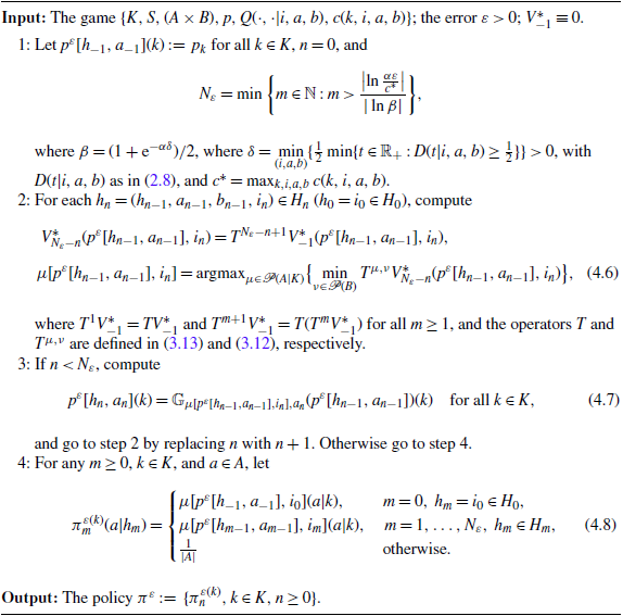
 ε
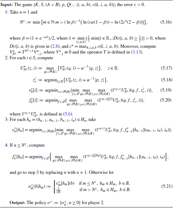
 ε


