2.1 Expectations survey data

The survey data are from the Joint Harmonised EU Programme Business and Consumer Survey (BCS) of the European Commission (EC). The data consists of a set of fully anonymized individual answers of the monthly consumer survey from January 2004 to December 2019. The survey is conducted by national institutes but shares a common timetable and a harmonized questionnaire across countries (European Commission, 2023). Most national institutes use a repeated cross-sectional sample. I restrict the analysis to the Euro Area and ten member countries due to data limitations for the other member states. Nonetheless, the sample includes countries that reflect the economic and geographical diversity of the monetary union.Footnote ¹

The questionnaire begins with a set of questions regarding the socioeconomic status, including age, gender, income, and education of the respondent. On average, 19,000 individuals participate each month in the Euro Area. For larger countries like Germany or Italy, there are on average about 1,700-1,900 respondents per month. For smaller countries, the monthly sample typically exceeds 1,000 individuals. The relevant survey question concerns respondents’ inflation expectations. In a first step, participants answer a qualitative question about whether they expect inflation to increase, decrease, or stay about the same over the next 12 months. Those who expect inflation to change are then asked the following question:

If a respondent indicates in the qualitative question that they expect inflation to stay the same, the survey administrator imputes a quantitative inflation expectation of zero for that respondent. To mitigate biases in household inflation expectation surveys – particularly those arising from extreme outliers – Arioli et al. (Reference Arioli, Bates, Dieden, Duca, Friz, Gayer, Kenny, Meyler and Pavlova2017) recommend applying asymmetric trimming to the most extreme responses. Therefore, I exclude responses exceeding 40% in absolute value, which removes approximately 28% of the right tail, while keeping the left tail unchanged. Further trimming is possible, but Arioli et al. (Reference Arioli, Bates, Dieden, Duca, Friz, Gayer, Kenny, Meyler and Pavlova2017) note that beyond 30% trimming, improvements are minimal.Footnote ²

Despite these biases, Arioli et al. (Reference Arioli, Bates, Dieden, Duca, Friz, Gayer, Kenny, Meyler and Pavlova2017) highlight key strengths of the survey data, including a strong consistency between qualitative and quantitative expectations and a high correlation between expected and realized inflation. The survey question is deliberately vague, allowing respondents to apply their own interpretation of the relevant consumption basket.

Previous findings suggest that demographic characteristics play an important role in the formation of inflation expectations. It has been shown that gender, income, marital status, education, and even cognitive abilities have a causal impact on inflation expectations (D’Acunto et al. Reference D’Acunto, Malmendier, Ospina and Weber2021, Reference D’Acunto, Malmendier, Weber, D’Acunto, Malmendier and Weber2023). To ensure that the results are not driven by socioeconomic characteristics such as age, gender, or income (D’Acunto et al. Reference D’Acunto, Charalambakis, Georgarakos, Kenny, Meyer and Weber2024) and to focus on cross-country heterogeneity within the Euro Area, I follow Fofana et al. (Reference Fofana, Patzelt and Reis2024) and residualize the inflation expectations. This is done by running the following regression separately for the Euro Area and each country:

(1) \begin{equation} \pi _{i,t}^{exp} = \beta _0 + \beta _1 age_{i,t} + \beta _2 educ_{i,t} + \beta _3 income_{i,t} + \beta _4 gender_{i,t} + \delta _{t} + \varepsilon _{i,t} \end{equation}

where $\pi _{i,t}^{exp}$ represent the 12-month ahead inflation expectations of survey respondents ( $i$ ) for every month ( $t$ ) from January 2004 to December 2019.

The measure of household inflation expectations is the time-fixed effect, $\delta _{t}$ , which is a residualized mean of inflation expectations, for every country and the Euro Area.Footnote ³

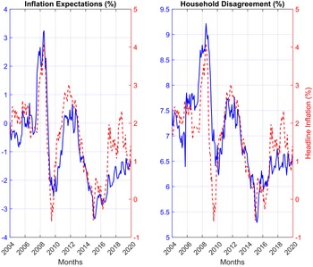
Furthermore, the standard deviation of the error term $\varepsilon _{i,t}$ measures the disagreement among households (Fofana et al. Reference Fofana, Patzelt and Reis2024). Incorporating a measure of disagreement takes into account that not all households have the same formation process for inflation expectations, and allows to analyze whether and how pronounced households disagree in response to a carbon policy shock. Previous research suggests that disagreement is time-varying and co-moves with key macroeconomic variables (Mankiw et al. Reference Mankiw, Reis and Wolfers2003). Following Mankiw et al. (Reference Mankiw, Reis and Wolfers2003), I define disagreement as the standard deviation of one-year-ahead inflation expectations across respondents within each country and the Euro Area. This differs from uncertainty, which reflects intrapersonal variation in expectations over time. Figure 1 shows the measure for inflation expectations and household disagreement for the Euro Area.

Figure 1.

Household inflation expectations and disagreement.

Notes: The left panel shows the time series of residualized household inflation expectations, and the right panel shows the measure of household disagreement for the Euro Area (left axis for both panels). As a reference, the headline inflation rate is included (red dotted line, right axis) in both graphs.

Figure 1. Long description

Two line graphs are presented side by side. Panel A on the left shows the time series of residualized household inflation expectations in percent on the left y-axis, ranging from -4 to 4 percent. The x-axis represents months from 2004 to 2020. A blue solid line represents the inflation expectations data. Panel B on the right shows the measure of household disagreement in percent on the left y-axis, ranging from 5 to 9.5 percent. The x-axis also represents months from 2004 to 2020. A blue solid line represents the household disagreement data. Both panels include a red dotted line representing the headline inflation rate on the right y-axis, ranging from -1 to 5 percent. The graphs illustrate the trends and fluctuations in household inflation expectations and disagreement over time, with the headline inflation rate provided as a reference.

As a reference, the annualized growth rate of the Harmonized Index of Consumer Prices (HICP) is plotted as well.Footnote ⁴ On average, inflation expectations surged in 2008, a period marked by high energy and food prices. This was followed by a sharp decrease of inflation expectations during the Great Recession in 2009. After 2012, during the Euro crisis and the zero lower bound period, inflation expectations gradually declined, reaching a trough in 2015. In line with the findings in Mankiw et al. (Reference Mankiw, Reis and Wolfers2003), inflation expectations and household disagreement co-move with the headline inflation rate.

2.2 The carbon policy shock

To study how carbon pricing impacts inflation expectations, I use the carbon policy shock series constructed by Känzig (Reference Känzig2026). Känzig (Reference Känzig2026) leverages the regulatory framework of the European Union Emission Trading System (EU ETS), the largest carbon market in the world, where European firms purchase certificates that allow them to emit greenhouse gases. He exploits unexpected regulatory changes that determine the supply of emission allowances by the EC. If these events cause changes in carbon future prices within a sufficiently tight window, then this change in carbon futures can be attributed to the unexpected regulatory announcement and is exogenous. The series is then refined by regressing it on a set of macroeconomic, financial, oil market, and climatic variables. This takes into account potential predictability of the surprise series.Footnote ⁵ This high-frequency refined surprise series is then employed as an instrument in a VAR model. Using an external instruments approach, he identifies the structural shocks. This allows Känzig (Reference Känzig2026) to extract the shock series from the VAR model, which I use for the empirical analysis.

4.1 Area-wide results

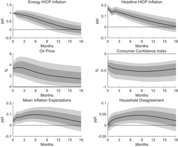
As a baseline, I present the impulse responses for the Euro Area in Figure 2, showing the dynamic effects of a carbon policy shock over a 18-month horizon. Following a carbon policy shock that raises energy inflation by one percentage point, the headline inflation rate increases for approximately a year, accompanied by a significant and pronounced decrease in consumer confidence, the forward-looking measure for economic activity. This is in line with the persistent impact on economic activity documented by Känzig (Reference Känzig2026) who finds that real GDP and especially consumption fall persistently while industrial production decreases. The prolonged impact on economic activity beyond the maximum horizon shown masks regional heterogeneity, as explored by other contributions (Berthold et al. Reference Berthold, Cesa-Bianchi and Di Pace2024; Mangiante, Reference Mangiante2024; Känzig and Konradt, Reference Känzig and Konradt2024).

Figure 2.

Dynamic effects of a carbon policy shock.

Notes: The shock impact is normalized to lead to a one percentage point increase in energy inflation. The figure shows the median responses (black lines) together with the 68% (dark gray) and 90% (light gray) error bands.

Inflation expectations display a significant increase in response to the carbon policy shock: households, on average, revise their expectations upward. This relationship is particularly noteworthy given that the sample period was characterized by low and stable inflation rates, and households were not directly targeted by the carbon pricing itself. Instead, they appear to react indirectly, through the energy cost channel - that is, via observed increases in consumer energy prices. Once the effect on headline and energy inflation fades out (after about 9 months), so does the effect on inflation expectations. In line with standard models of information rigidities (Coibion and Gorodnichenko, Reference Coibion and Gorodnichenko2012), the response is hump-shaped, reflecting that household expectations adjust only gradually relative to the immediate increase in headline inflation. While the response of inflation peaks on impact, inflation expectations reach their maximum response only after six months. This pattern is consistent with previous findings for the Euro Area using qualitative survey data of household inflation expectations. For example, Geiger et al. (Reference Geiger, Gründler and Scharler2023) document a peak after six months in response to a monetary policy shock, while Baumeister (Reference Baumeister2023) finds a peak after eleven months in response to an oil supply shock. Quantitatively, average inflation expectations increase by up to 0.1 percentage points following a carbon policy shock that raises headline inflation by approximately 0.2 percentage points on impact, underscoring the sensitivity of household inflation expectations to carbon pricing.

Disagreement among households rises gradually after the shock and peaks after around eight months at approximately 0.05 percentage points. This delayed and persistent increase suggests that not all households adjust their expectations simultaneously, consistent with the idea of slow information diffusion. This finding aligns with earlier evidence that inflation disagreement tends to increase during periods of rising prices (Mankiw et al. Reference Mankiw, Reis and Wolfers2003). One possible explanation is that households update their expectations infrequently or based on heterogeneous information sets – a mechanism captured by sticky or noisy information models (Mankiw and Reis, Reference Mankiw and Reis2002).

The main takeaway is that the rise in household inflation expectations is both significant and persistent. Importantly, this average increase is accompanied by a significant rise in disagreement across households, highlighting heterogeneity in how the inflationary shock is perceived and mapped into expectations.

Figure 3.

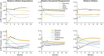
Dynamic effects of a carbon policy shock by country, relative to the Euro area.

Notes: The figure displays impulse responses of inflation expectations, household disagreement, and inflation to a normalized carbon policy shock, shown by country relative to the median response for the Euro Area. For each horizon, I compute the difference between a country’s response and the Euro Area response, such that the Euro Area is normalized to zero. Horizons where the difference is statistically significant at the 68% confidence level are marked with an $\times$ .

Figure 3. Long description

The image contains six line graphs showing the dynamic effects of a carbon policy shock by country relative to the Euro area. Each graph represents different metrics: Relative Inflation Expectations, Relative Household Disagreement, and Relative Inflation. The graphs are divided into two rows, each containing three graphs. The x-axis for all graphs represents time in months, ranging from 0 to 18. The y-axis represents the difference in impulse responses (Δ IRF) between individual countries and the Euro Area (EA) in percentage points (ppt). Each graph includes multiple lines representing different countries, with legends indicating which line corresponds to which country. The graphs show how the responses to a carbon policy shock vary by country over time. Statistically significant differences at the 68% confidence level are marked with an asterisk (*).

4.2 Cross-country heterogeneity

While the aggregate results offer a useful overview of how households adjust their inflation expectations in response to a carbon policy shock, they may mask important cross-country differences. Understanding this heterogeneity in the expectation formation process is crucial for policymakers, especially as central banks aim to keep inflation expectations anchored following energy-driven inflationary shocks. I begin by analyzing differences in the magnitude of the responses across countries, comparing how both inflation expectations and disagreement vary. I then examine the timing of these responses by comparing the month at which headline inflation and inflation expectations each reach their peak. Beyond the common pattern of a delayed expectations response relative to the immediate price increase, the number of months separating the two peaks varies meaningfully across countries.

The left panel of Figure 3 displays the median impulse responses of inflation expectations for individual Euro Area member states, obtained from separately estimated VAR models using the carbon policy shock as the instrument. The shock is normalized to generate a one percentage point increase in Euro Area energy inflation. Each country’s response is expressed relative to the median Euro Area response by subtracting it from the country IRF. To facilitate comparison, countries are divided into two panels: the four largest economies and a second group of the six smaller economies. Horizons at which the median response differs significantly from the Euro Area are indicated with crosses, based on 68% error bands.Footnote ¹⁰

Two main findings stand out. First, there is some heterogeneity across countries: deviations from the Euro Area response generally lie within a band of 0.1 percentage points. While this range is relatively narrow, it is noteworthy given that the inflationary impulse of the normalized shock is only about 0.2 percentage points on impact, and the sample period is characterized by relatively low and stable inflation rates. Second, the relative response of average inflation expectations (left panel in Figure 3) tends to closely track the relative response of actual inflation (right panel in Figure 3) – countries experiencing a stronger inflationary impact from the carbon policy shock also tend to exhibit a larger increase in expectations. The pattern holds particularly well for the larger economies. A notable exception is Germany, where inflation expectations and disagreement both exceed the Euro Area response by approximately 0.05 percentage points throughout the horizon, despite an inflation response that is virtually identical to the aggregate. Further exceptions include some smaller economies such as Luxembourg, where the relative inflation response is more pronounced, but not tracked by the expectations response. Statistically significant negative deviations from the Euro Area expectations response are observed for Germany, Spain, Slovenia, Luxembourg, and Finland. The most pronounced positive deviation is found for Slovenia, where inflation expectations increase on impact by 0.15 percentage points more than on average in the Euro Area.

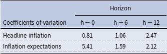
To quantify and compare heterogeneity across countries, I use the coefficient of variation (CoV), a standard measure of relative dispersion. Following Corsetti et al. (Reference Corsetti, Duarte and Mann2022), the coefficient of variation is defined as the ratio of the standard deviation to the mean and captures the extent of heterogeneity relative to the average response. Specifically, I compute the standard deviation of the median impulse responses across countries relative to the Euro Area median response at each horizon, as in Geiger et al. (Reference Geiger, Gründler and Scharler2023).Footnote ¹¹ For consistency, I normalize the Euro Area response to unity in absolute value. Table 1 reports the resulting coefficients of variation for selected horizons.

Table 1.

Coefficients of variation for inflation and inflation expectations for selected horizons

Table 1. Long description

A table with two rows and four columns. The columns are labeled ‘Coefficients of variation’ and ‘Horizon’ with sub-columns ‘h = 0’, ‘h = 6’, and ‘h = 12’. The row labels are ‘Headline inflation’ and ‘Inflation expectations’. Row 1: Headline inflation, 0.81, 1.06, 2.47. Row 2: Inflation expectations, 5.41, 1.59, 2.12. The table shows the coefficients of variation for headline inflation and inflation expectations at different horizons.

The coefficients indicate greater heterogeneity in the response of inflation expectations compared to inflation itself. This aligns with Geiger et al. (Reference Geiger, Gründler and Scharler2023), who find that expectations exhibit more variation following a monetary policy shock than the consumer price index. The on-impact variation for the median responses is 5.41 for inflation expectations, while it is only 0.81 for inflation.Footnote ¹² The CoV for inflation expectations declines notably after the initial on-impact heterogeneity, whereas the coefficient for headline inflation remains relatively stable and even increases. After approximately one year, the CoV indicates that the degree of heterogeneity converges across expectations and actual inflation.

Countries may differ not only in the average response of inflation expectations but also in the degree of household disagreement in response to a carbon policy shock. The middle panel of Figure 3 displays the impulse responses of household disagreement to a normalized carbon policy shock. Across all countries, relative disagreement evolves in a pattern similar to that of relative inflation expectations. Countries with a smaller increase in inflation expectations relative to the Euro Area also tend to exhibit a less pronounced rise in disagreement. The cumulative impacts on the mean and the standard deviation of expectations are highly correlated, with a coefficient of approximately 0.87 (p-value = 0.001).Footnote ¹³ For instance, both Slovenia and Spain show large increases in inflation expectations, accompanied by similarly large increases in household disagreement. These results indicate that carbon policy shocks lead to increases not only in the level of inflation expectations but also in the dispersion of beliefs. The strong cross-country correlation between these two responses suggests that larger shifts in average expectations are associated with greater heterogeneity in how households perceive and process the shock.

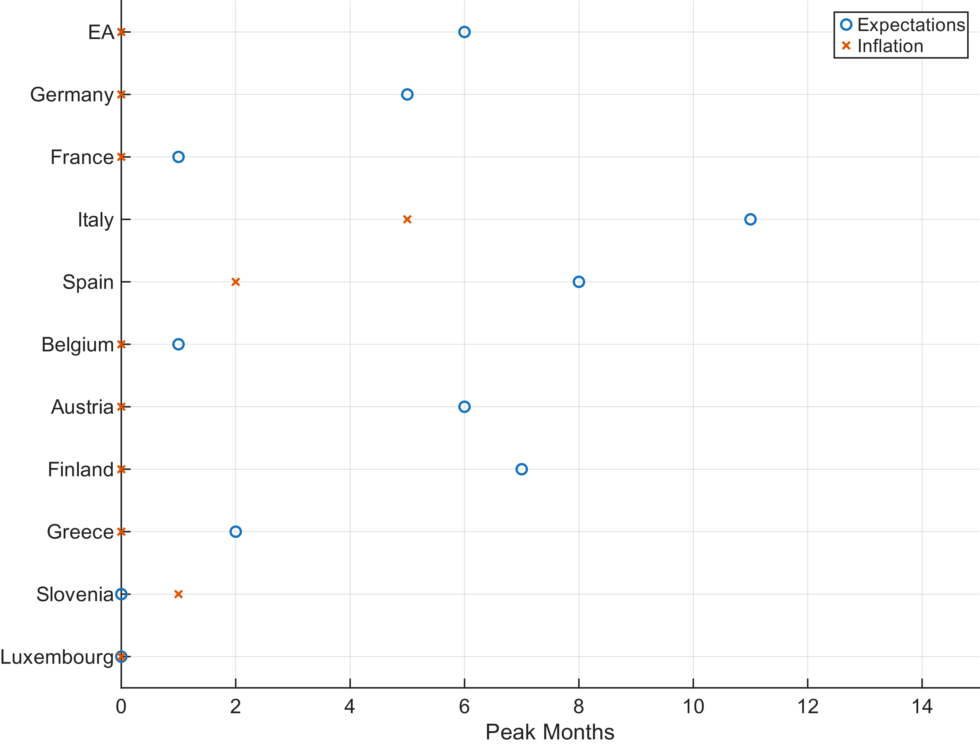
Another dimension of cross-country heterogeneity emerges when examining the timing of the peak response values for inflation expectations and the inflation rate, as shown in Figure 4.

The timing of peak inflation is relatively consistent across countries, with most reaching their maximum inflation response on impact or shortly after – except for Italy, where the peak occurs after around five months. In contrast, the peak response in inflation expectations is generally later and exhibits greater cross-country variation. At the Euro Area level, expectations peak after six months – a pattern closely mirrored only by Germany, Austria, and Finland. In most countries, inflation expectations reach their peak after the inflation rate itself, a pattern that aligns well with models of information frictions, such as the sticky information framework (Mankiw and Reis, Reference Mankiw and Reis2002; Coibion and Gorodnichenko, Reference Coibion and Gorodnichenko2012). This delay suggests that households do not adjust their expectations immediately in response to the policy shock but do so gradually as (energy) price increases materialize and become more salient in day-to-day life.

Figure 4.

Peak months of inflation expectations and inflation.

Notes: The figure compares the months of the peak responses for both inflation expectations and the headline inflation following a carbon policy shock. Each point represents the month in which the peak response is observed, highlighting the differences in timing across countries.

The heterogeneity in response timing has implications for monetary policy. Since policy effectiveness often hinges on inflation expectations remaining well-anchored (Baumeister, Reference Baumeister2023), understanding when households revise their expectations following cost-push shocks is relevant for central banks assessing whether and how to respond. Across most countries, the peak expectation response lags the peak inflation response by five to seven months. Luxembourg, Belgium, and France are notable exceptions, with a lag of less than one month, while Slovenia is the only country where the expectation response peaks before headline inflation does.

4.3 Comparison with an oil supply news shock

To assess whether the cross-country pattern documented above reflects a specific expectations response induced by carbon policy shocks or a more general response to energy price shocks, I benchmark the results against the response to an oil supply news shock (Känzig, Reference Känzig2021).Footnote ¹⁴ Oil price shocks are a well-documented driver of household inflation expectations (Coibion and Gorodnichenko, Reference Coibion and Gorodnichenko2015; Wong, Reference Wong2015; Aastveit et al. Reference Aastveit, Bjørnland and Cross2023; Baumeister, Reference Baumeister2023). Comparing the two responses is informative about the role of the energy price channel: if households react to the inflationary implications of a shock rather than its specific origin, the responses should look similar. I find that this is indeed the case — the two shocks generate expectations responses that are similar in shape and timing, with level differences proportional to the respective price effects.

Figure 5.

Comparison of the effects with an oil supply news shock.

Notes: This figure presents the median response of inflation expectations alongside the 90 % error bands for each country. The carbon policy shock is depicted in red (dashed line), while the oil supply news shock is shown in blue (solid line). Both shocks are normalized to imply a one percentage point increase in the Euro Area energy inflation rate.

I analyze the effects of the oil supply news shock from Känzig (Reference Känzig2021) using the same empirical framework as before, replacing only the instrument in the internal instruments SVAR.Footnote ¹⁵ The shock is again normalized to generate a one percentage point increase in Euro Area energy inflation on impact, ensuring comparability across shocks. Figure 5 compares the dynamic responses of inflation expectations to both shocks across countries.

Figure 6.

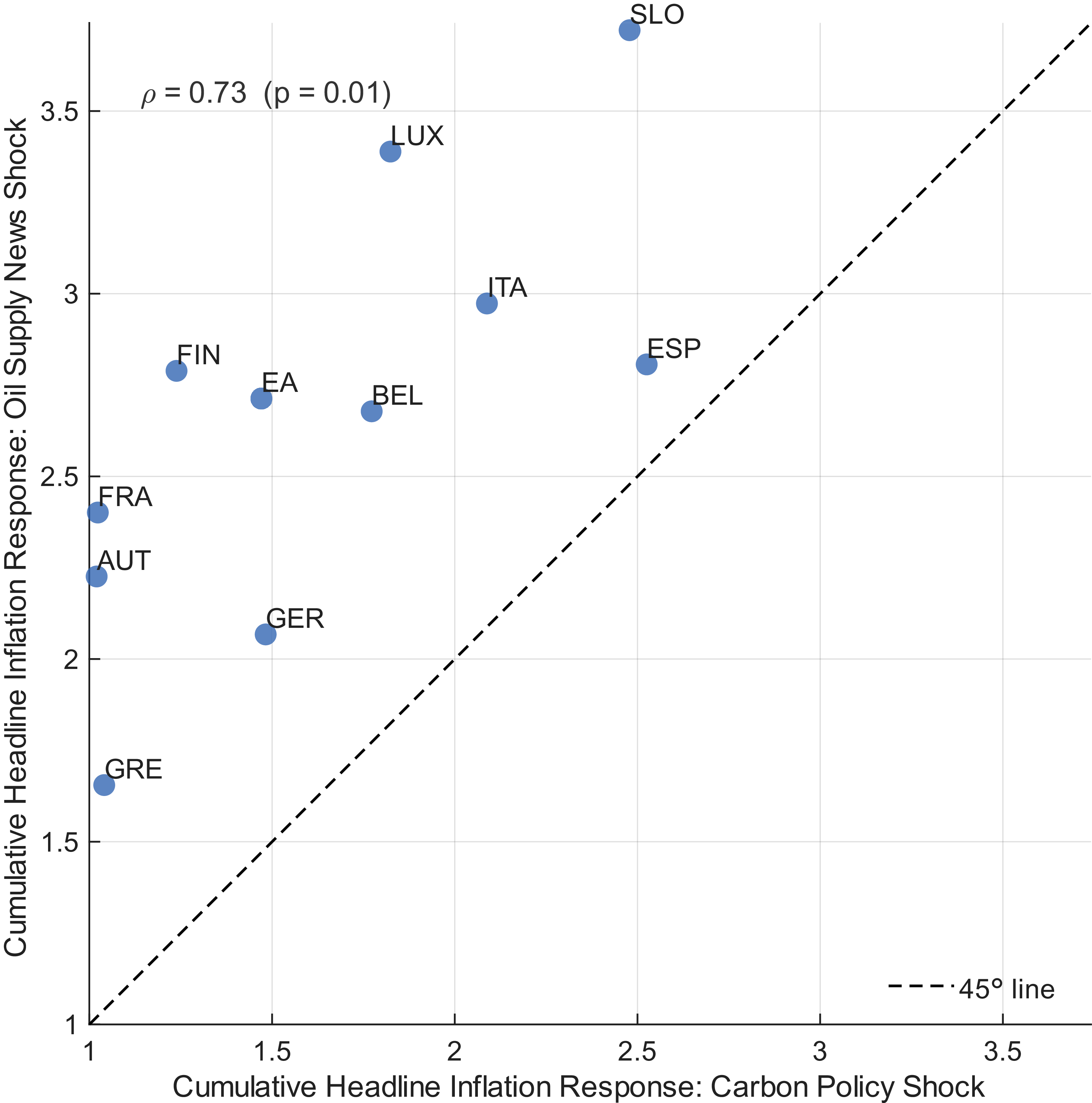
Cumulative response of headline inflation to both shocks.

Notes: Cumulative median headline inflation response over 18 months to a carbon policy shock (x-axis) and an oil supply news shock (y-axis), both normalized to a one percentage point increase in Euro Area energy inflation on impact. Points above the 45-degree line indicate a stronger cumulative response to the oil supply news shock.

The shape and timing of the responses are similar across both shocks. For Spain, Austria, and Finland, the peak response occurs in the same month; and for most of the other countries they are typically close to each other. Overall, for six out of ten countries the peak months differ by no more than two months.Footnote ¹⁶ Further, the cross-country peak responses to the two shocks are highly correlated, with a correlation coefficient of about 0.84 – countries that respond more strongly to the carbon policy shock tend to do so also following an oil supply news shock.Footnote ¹⁷

The level of the responses, however, differs. The peak impact on inflation expectations following an oil supply news shock is approximately 1.5 to two times larger than following a carbon policy shock – for the Euro Area, the peak response is approximately 0.2 percentage points, roughly twice the peak response after a carbon policy shock. This differential is consistent with the stronger headline inflation pass-through documented in Figure 6, plotting the cumulative headline inflation response to both shocks against each other.

All countries lie above the 45-degree line, illustrating that the oil supply news shock generates a larger cumulative headline inflation response across all countries in the sample. For the Euro Area, the cumulative headline inflation response to the oil supply news shock is approximately 2.75 percentage points – roughly twice the 1.5 percentage points following a carbon policy shock, a ratio that closely mirrors the relative difference in inflation expectations responses. The level difference in expectations is therefore proportional to the difference in realized price effects, suggesting that the (energy) price channel might be the dominant driver.

Beyond the inflation response, the oil price dynamics also differ strikingly: the oil supply news shock raises oil prices by around 10% on impact, compared with only about 3% following the carbon policy shock. Since household inflation expectations are sensitive to salient gasoline prices (Coibion and Gorodnichenko, Reference Coibion and Gorodnichenko2015; Wong, Reference Wong2015; Coibion and Gorodnichenko, Reference Coibion and Gorodnichenko2025), the smaller oil price response following a carbon policy shock translates into a weaker and less visible price signal for households – consistent with a more muted expectations response.Footnote ¹⁸

Taken together, the similarity in expectations responses across the two shocks suggests that households respond to the implied price effects of an energy shock rather than to its specific origin. This points naturally to the energy price channel as a potential mechanism underlying the cross-country heterogeneity documented above.

5.1 Cross-country evidence

Even though I control for socioeconomic characteristics that influence the formation of inflation expectations, a substantial degree of heterogeneity remains across countries. In the left graph of Panel A in Figure 7, I plot the peak inflation expectations response against the average energy weight in the country HICP basket, finding a significant positive correlation with a coefficient of approximately 0.6. Given that the HICP is constructed as a weighted index of consumer goods and services, a higher energy weight implies greater direct exposure to energy price fluctuations, which might be leading to a stronger reaction in inflation expectations. For instance, Germany, Spain, and Slovenia – each with an energy share of around 11% or higher – display notably larger peak responses than Austria, Italy, Finland, or Greece, where energy accounts for only about 8% of the consumption basket. This is consistent with evidence that household inflation expectations respond more or less proportional to the energy expenditure shares in their basket (Binder, Reference Binder2018).

To investigate this further, I estimate relative impulse responses, splitting the country group in the half with the larger energy weight (Slovenia, Germany, Spain, Luxembourg, and Belgium) and the remaining countries, using the following panel local projection model (Jordà, Reference Jordà2005):

(3) \begin{equation} \pi _{c,t+h}^{exp} = \alpha _{c,h} + \beta _h s_t + \gamma _h (s_t \times g_c)+ \sum _{p=1}^{6} \delta _{p,h}' \mathbf{X}_{c,t-p} + \varepsilon _{c,t+h}, \end{equation}

where $s_t$ is the carbon policy shock, $\alpha _{c,h}$ are country fixed effects, and $g_c$ is an indicator equal to one for the five countries with the largest energy share. The control vector $\mathbf{X}$ includes up to six lags of the dependent variable, $\pi _{c,t+h}^{exp}$ , headline inflation, energy inflation, oil prices, and consumer confidence. I select the lag length of the local projection model following the insights of Ludwig (Reference Ludwig2024) that the forecast of a local projection of order $p$ estimated through horizon $h$ corresponds to a sequence of one-step ahead forecasts from VAR models of increasing order up to $p + h - 1$ . Therefore with $p = 6$ and $H = 12$ , this implies a VAR order of up to 17, well aligned with the 18-lag BVAR estimated for the baseline results. The differential impulse response is captured by the sequence of coefficients $\gamma _h$ , with inference based on a wild cluster bootstrap with Webb weights, two-way clustered at the country and time level (Roodman et al. Reference Roodman, Nielsen, MacKinnon and Webb2019).

The left graph of Panel B in Figure 7 shows the differential impulse responses, which are for almost all horizons positive and reach up to 0.1 percentage points at horizons four to eight, statistically significant at the 68% level. This constitutes suggestive evidence that differences in the energy consumption share are a key channel through which carbon policy shocks differentially affect inflation expectations – consistent with the well-established finding that households rely on frequently observed prices, and energy prices in particular, when forming their inflation expectations (D’Acunto et al. Reference D’Acunto, Malmendier, Weber, D’Acunto, Malmendier and Weber2023; Coibion and Gorodnichenko, Reference Coibion and Gorodnichenko2025).

Figure 7.

Explaining cross-country heterogeneity in inflation expectations.

Notes: Panel A shows the cross-country correlation between (left) the average energy weight in the HICP basket (2004–2019) and the peak response of inflation expectations, and (right) the peak response of consumer confidence and the peak response of inflation expectations. Panel B displays the differential impulse responses from a panel local projection (equation 3), estimated for the high-exposure group versus the remaining countries. Responses are normalized to a one percentage point increase in EA energy inflation on impact. The confidence intervals are computed using a wild cluster bootstrap with Webb weights, two-way clustered at the country and time level, and are shown at the 68 % and 90 % confidence level (Roodman et al. Reference Roodman, Nielsen, MacKinnon and Webb2019).

Consumer confidence

Another striking pattern in the results is the strong negative correlation between the peak consumer confidence response and the peak inflation expectations response across countries, visible in the right graph of Panel A in Figure 7: countries where consumer confidence deteriorates more sharply following the carbon policy shock also display stronger upward revisions in inflation expectations. The correlation coefficient is $-0.66$ .Footnote ¹⁹

This pattern is consistent with findings in the literature. Kamdar and Ray (Reference Kamdar and Ray2024) document a stagflationary belief correlation – an empirical pattern where consumers who expect higher unemployment also expect higher inflation. They propose a model of rational inattention in which individuals, facing costly information acquisition, allocate attention toward more relevant shocks. Because supply-driven recessions are especially costly for households that rely on labor income, consumers rationally devote more attention to supply shocks than to demand shocks; as a result, inflation is perceived as countercyclical. This mechanism helps explain why pessimistic consumers expect higher inflation while optimistic ones do not, suggesting a systematic link between consumer confidence and inflation expectations.

I compute again relative impulse responses using the panel local projection model (3), setting $g_c = 1$ for the four countries with the strongest consumer sentiment decline – Spain, Slovenia, France, and Luxembourg.Footnote ²⁰ The right graph of Panel B in Figure 7 shows the differential impulse response, which is around 0.1 percentage points and is statistically significant at the 68% level for the the months three to eight.

The co-movement of inflation expectations and sentiment complements recent work on the geographic effects of carbon pricing on economic activity. Mangiante (Reference Mangiante2024) finds that poorer regions – more prevalent in countries such as Spain and Slovenia – are disproportionately affected by carbon policy shocks, experiencing larger contractions in output. Since consumer sentiment is a forward-looking indicator of economic conditions, the stronger rise in inflation expectations observed in these countries may also reflect the influence of worsening economic prospects on expectations.

5.2 A price channel decomposition

To quantify how much of the aggregate response is driven by the direct energy price channel, I follow Holm et al. (Reference Holm, Paul and Tischbirek2021) and Mangiante (Reference Mangiante2026), and augment the panel local projection model with leads of energy inflation, thereby decomposing the direct shock effect from the portion that works through the energy price path. Specifically, I estimate:

(4) \begin{equation} \pi _{c,t+h}^{exp} = \alpha _{c,h} + \beta _h s_t+ \sum _{p=1}^{6} \delta _{p,h}' \mathbf{X}_{c,t-p}+ \sum _{m=0}^{h} \phi _{m,h} v_{c,t+m} + \varepsilon _{c,t+h}, \end{equation}

where $v_{c,t+m}$ represents the leads of energy inflation.Footnote ²¹ The number of horizons, control variables, and lags is the same as in equation (3). I estimate the sequence of coefficients $\beta _h$ both without and with the energy inflation leads, and interpret the difference as the contribution of the direct price channel. Figure 8 presents the impulse responses of inflation expectations (top-left panel), household disagreement (top-right panel), and consumer confidence (bottom-left panel) under each specification.

Figure 8.

Price-channel decomposition of household responses.

Notes: The figure shows impulse responses from the panel local projection model (4), estimated without energy inflation leads (Baseline IRF, blue solid) and conditional on energy inflation leads (Direct Effects, red dashed). The top-left panel shows the response of inflation expectations, the top-right panel the response of household disagreement, and the bottom-left panel the response of consumer confidence. Responses are normalized to a one percentage point increase in EA energy inflation on impact. Confidence intervals are computed using a wild cluster bootstrap with Webb weights, two-way clustered at the country and time level, and are shown at the 68 % and 90 % confidence level (Roodman et al. Reference Roodman, Nielsen, MacKinnon and Webb2019).

Figure 8. Long description

The image contains three line graphs showing the responses of different economic indicators to a one percentage point increase in energy inflation. Panel A: The top-left graph shows the response of inflation expectations over 12 months. The y-axis represents the change in inflation expectations in percentage points (ppt), and the x-axis represents time in months. The blue solid line represents the baseline impulse response function (IRF), while the red dashed line represents the direct effects. The shaded areas around the lines indicate confidence intervals at the 68 percent and 90 percent levels. Panel B: The top-right graph shows the response of household disagreement over 12 months. The y-axis represents the change in household disagreement in percentage points (ppt), and the x-axis represents time in months. The blue solid line represents the baseline IRF, while the red dashed line represents the direct effects. The shaded areas around the lines indicate confidence intervals at the 68 percent and 90 percent levels. Panel C: The bottom-left graph shows the response of consumer confidence over 12 months. The y-axis represents the change in consumer confidence in percent (%), and the x-axis represents time in months. The blue solid line represents the baseline IRF, while the red dashed line represents the direct effects. The shaded areas around the lines indicate confidence intervals at the 68 percent and 90 percent levels.

Strikingly, once energy price dynamics are controlled for, the impulse responses for inflation expectations, household disagreement, and consumer confidence are close to zero and statistically insignificant throughout the horizon. This indicates that the carbon policy shock affects household expectations and sentiment almost exclusively through its pass-through into energy prices, rather than through any additional direct policy channel. The finding is consistent with Mangiante (Reference Mangiante2026), who documents that the energy price pass-through is also the dominant channel for the expectations response of Italian firms to carbon policy shocks.