



1. Introduction
Passive control of wall-bounded turbulence by rough or textured surfaces has long been studied as a means of modifying near-wall coherent motions and, in turn, friction drag or transport efficiency in canonical flows such as turbulent channel flow and Taylor–Couette (TC) flow (Nikuradse Reference Nikuradse1933; Schlichting Reference Schlichting1937; Rothstein Reference Rothstein2010; Srinivasan et al. Reference Srinivasan, Kleingartner, Gilbert, Cohen, Milne and McKinley2015; Bottaro Reference Bottaro2019). Two closely related objectives are pursued: (i) elucidating the multiscale mechanism whereby micro-features alter macro-flows and friction drag (Orlandi et al. Reference Orlandi, Leonardi and Antonia2006; Nepf Reference Nepf2012; Park et al. Reference Park, Choi and Kim2021; Chung et al. Reference Chung, Hutchins, Schultz and Flack2021); (ii) developing simplified models of effective boundaries for reliable prediction (Kamrin et al. Reference Kamrin, Bazant and Stone2010; Forooghi et al. Reference Forooghi, Stroh, Magagnato, Jakirlić and Frohnapfel2017; Bottaro Reference Bottaro2019; Ahmed & Bottaro Reference Ahmed and Bottaro2025; Gao et al. Reference Gao, Xie and Lu2025), efficient simulation (Aupoix & Spalart Reference Aupoix and Spalart2003; Aupoix Reference Aupoix2014; Lācis et al. Reference Lācis, Zampogna and Bagheri2017; Lācis et al. Reference Lācis, Sudhakar, Pasche and Bagheri2020) and optimisation of the energy-saving strategies (Luchini et al. Reference Luchini, Manzo and Pozzi1991; Bechert et al. Reference Bechert, Bruse, Hage, van der Hoeven and Hoppe1997; Rastegari & Akhavan Reference Rastegari and Akhavan2015; Endrikat et al. Reference Endrikat, Modesti, García-Mayoral, Hutchins and Chung2021). As such, this two-fold aim, encompassing both mechanism elucidation and model development, constitutes the central focus of the present study.
Firstly, the control mechanism of engineered surfaces (e.g. riblets, superhydrophobic textures) is attributed to boundary slip before near-wall inertial effects emerge as turbulence intensifies, a shift evidenced by their drag reduction (DR) performance and parametric dependence in previous research. For riblet (longitudinal groove) surfaces, DR depends strongly on the Reynolds number
 $ \textit{Re}$
and the lateral spacing w. An optimal DR of approximately
 $10\,\%$
is typically achieved in channel flows with
 $w^+\simeq 17$
(measured in wall units). In this drag-reducing regime, the anisotropic slip on the effective boundary dampens near-wall turbulent momentum transfer by impeding the lateral movement of quasi-streamwise vortices (Luchini et al. Reference Luchini, Manzo and Pozzi1991; Bechert et al. Reference Bechert, Bruse, Hage, van der Hoeven and Hoppe1997). Conversely, for larger spacings (
 $w^+\gt 30$
), DR deteriorates and gives way to drag increase, as inertial mechanisms overwhelm the slip effects. These inertial effects manifest as increased wall permeability and sloshing motions (Bechert et al. Reference Bechert, Bruse, Hage, van der Hoeven and Hoppe1997; Lācis et al. Reference Lācis, Sudhakar, Pasche and Bagheri2020) or breakdown of the viscous regime with enhanced Kelvin–Helmholtz (KH) instability (García-Mayoral & Jiménez Reference García-Mayoral and Jiménez2011; Zhu et al. Reference Zhu, Ostilla-Mónico, Verzicco and Lohse2016; Endrikat et al. Reference Endrikat, Modesti, García-Mayoral, Hutchins and Chung2021).
In contrast to solid walls, multiphase textured/patterned surfaces, such as superhydrophobic surfaces, have been developed to obtain a substantial and sustained DR, permitting large effective slip due to air or lubricant trapped within microscopic surface textures and cavities (Rothstein Reference Rothstein2010). In TC flow, for instance, a DR of approximately
 $22\,\%$
has been reported over superhydrophobic surfaces with random roughness (Srinivasan et al. Reference Srinivasan, Kleingartner, Gilbert, Cohen, Milne and McKinley2015). Unfortunately, under intense turbulent fluctuations, DR results over superhydrophobic surfaces become inconsistent and attenuated due to the deterioration or depletion of the air plastron (Park et al. Reference Park, Sun and Kim2014, Reference Park, Choi and Kim2021). The patterned slip wall is therefore designed not only to augment the magnitude of DR, but also to stabilise the gas–liquid interface via designed pinning sites (Hu et al. Reference Hu2017; Yu et al. Reference Yu, Li, McClelland, del Campo Melchor, Lee, Lee and Kim2023; Liu et al. Reference Liu2024). For longitudinal superhydrophobic grooves, it has been noted that the slip effect increases with increasing
 $w^+$
and decreasing solid fraction
 $\phi _s$
before the failure of air layers (Zhang et al. Reference Zhang, Tian, Yao, Hao and Jiang2015; Rastegari & Akhavan Reference Rastegari and Akhavan2019; Li et al. Reference Li, Ji, Tan, Li, Xiang, Lv and Duan2020). Drag reduction of up to
 $75\,\%$
has been reported in laboratory-scale experiments with
 $\phi _s=0.05$
in turbulent boundary layer flows (Park et al. Reference Park, Sun and Kim2014). In TC turbulence, Liu et al. (Reference Liu2024) reported a monotonic increase in DR with
 $w^+$
of up to
 $62\,\%$
at
 $w^+$
reaching
 $75$
. Thus, to explore the potential for greater DR under more intensified turbulence, it is desirable to further extend our understanding of the patterned slip surfaces in the regime of larger
 $w^+$
.
Although strong interfacial slip generally favours DR, inertial effects emerge for large
 $w^+$
in patterned slip cases, analogous to that in riblet walls. In turbulent channel flows, enhanced turbulent mixing and secondary flows significantly counteract the slip effects (Türk et al. Reference Türk, Daschiel, Stroh, Hasegawa and Frohnapfel2014). Rastegari & Akhavan (Reference Rastegari and Akhavan2019) also attribute the underestimation of slip length compared with the proposed scaling to wetting transition and inertial KH instability of the gas–liquid interfaces. Similar secondary structures have also been observed in TC turbulence and influence the large-scale Taylor rolls (Jeganathan et al. Reference Jeganathan, Shannak, Alba and Ostilla-Mónico2023). However, the formation and distortion of these secondary vortices, their role in the self-sustaining process of wall-bounded turbulence and their interaction with large-scale structures remain insufficiently understood. Resolving these multiscale vortex dynamics is essential for clarifying the inertial mechanisms and developing higher-order models for patterned slip surfaces.
Secondly, beyond the elucidation of wall-induced turbulent structures and the inertial-flow mechanism, another critical challenge remains in translating these insights into effective slip boundary conditions and predictive turbulence statistics. Given the inherent multiscale nature of the boundary-turbulence system, developing effective macroscale boundaries instead of full-scale analysis is critical for both prediction and optimisation (Park et al. Reference Park, Choi and Kim2021; Chung et al. Reference Chung, Hutchins, Schultz and Flack2021; Ahmed & Bottaro Reference Ahmed and Bottaro2025). Generally, the multiscale correlation consists of two components, i.e. the abstraction of effective boundaries from microscale geometry and their subsequent integration into macro-flow prediction.
On the one hand, to bridge the gap between micro-textures and effective coefficients, several methods have proven effective. For example, Stokes-flow solutions (Kamrin et al. Reference Kamrin, Bazant and Stone2010; Chang et al. Reference Chang, Jung, Choi and Kim2019; Ji et al. Reference Ji, Li, Du, Lv and Duan2023) provide an effective slip length
 $b$
or slip velocity
 $U_s$
at lower
 $ \textit{Re}$
, while asymptotic homogenisation theories serve as a rigorous framework for deriving these effective coefficients, applicable to complex surfaces involving roughness (Zampogna et al. Reference Zampogna, Magnaudet and Bottaro2019a
), porous substrates (Bottaro Reference Bottaro2019) and even compliant walls (Zampogna et al. Reference Zampogna, Naqvi, Magnaudet and Bottaro2019b
). Under higher turbulence, slip effects are quantified through magnitude estimates for
 $U_s$
or the roughness function
 $\Delta U^+$
scaled with micro-features (Seo & Mani Reference Seo and Mani2016; Rastegari & Akhavan Reference Rastegari and Akhavan2019; Berghout et al. Reference Berghout, Bullee, Fuchs, Scharnowski, Kähler, Chung, Lohse and Huisman2021; Liu et al. Reference Liu2024). Furthermore, when inertial effects are considered, additional coefficients are required to model higher-order statistics. For example, Reynolds stress can be parametrised by turbulent viscosity
 $\nu _t$
, which successfully describes the inertial advection in both developed channel (Türk et al. Reference Türk, Daschiel, Stroh, Hasegawa and Frohnapfel2014) and TC turbulence over patterned walls (Brauckmann & Eckhardt Reference Brauckmann and Eckhardt2013; Xu et al. Reference Xu, Su, Lan, Zhao, He, Sun and Wang2023). Türk et al. (Reference Türk, Daschiel, Stroh, Hasegawa and Frohnapfel2014) further obtained the distribution
 $\nu _t$
through empirical relations and revealed its counteracting effect on the wall slip.
On the other hand, much work has been done concerning how to relate the effective coefficients to macro-flows. The drag decomposition quantifies contributions from slip effects and turbulence modifications (Fukagata et al. Reference Fukagata, Iwamoto and Kasagi2002; Rastegari & Akhavan Reference Rastegari and Akhavan2015, Reference Rastegari and Akhavan2018). For developed turbulent boundary layers over slip boundaries, the relation between friction drag and wall slip can be derived from integrated logarithmic profiles (Rastegari & Akhavan Reference Rastegari and Akhavan2018). Similarly in turbulent TC flows, Srinivasan et al. (Reference Srinivasan, Kleingartner, Gilbert, Cohen, Milne and McKinley2015) proposed a slip-modified friction law based on the angular-momentum defect theory of Panton (Reference Panton2007). As for the inertial effects, explicit models remain scarce. The inertial coefficients are typically employed as qualitative descriptions, such as for attenuated nonlinear slip (Türk et al. Reference Türk, Daschiel, Stroh, Hasegawa and Frohnapfel2014), or incorporated into empirical closure equations in Reynolds-averaged Navier–Stokes simulations extended to rough/textured walls (Aupoix & Spalart Reference Aupoix and Spalart2003; Lasagna et al. Reference Lasagna, Zampino and Ganapathisubramani2024). Therefore, greater efforts are warranted to parameterise effective boundaries and establish the explicit multiscale correlations between micro-textures, effective coefficients and macro-flows, especially when higher-order inertial effects amplify in higher turbulence.
Viewed more broadly, effective-boundary modelling for high-
 $ \textit{Re}$
applications follows a clear progression towards higher-order descriptions. At low inertia, the modelling is primarily boundary-centred and one-way: the surface geometry and interfacial properties are reduced to linear response parameters, such as an effective slip length
 $b$
or slip velocity
 $U_s$
, which are then imposed on the outer flow (Luchini et al. Reference Luchini, Manzo and Pozzi1991; Kamrin et al. Reference Kamrin, Bazant and Stone2010; Rothstein Reference Rothstein2010; Rastegari & Akhavan Reference Rastegari and Akhavan2019; Crowdy Reference Crowdy2021). As
 $ \textit{Re}$
and
 $w^+$
increase, however, the boundary-generated convective motions and vortical structures feed back on the effective response, so that higher-order moments and nonlinear inertial terms can no longer be neglected (Bechert et al. Reference Bechert, Bruse, Hage, van der Hoeven and Hoppe1997; García-Mayoral & Jiménez Reference García-Mayoral and Jiménez2011; Aupoix Reference Aupoix2014; Türk et al. Reference Türk, Daschiel, Stroh, Hasegawa and Frohnapfel2014; Bottaro Reference Bottaro2019; Ahmed & Bottaro Reference Ahmed and Bottaro2025). Formally, this transition is reflected in the increasing importance of higher-order nonlinear terms in both analysis and modelling. For example, apart from the linear slip terms, Ahmed & Bottaro (Reference Ahmed and Bottaro2025) considered second-order asymptotic models during homogenisation that retain the inertial term
 $\boldsymbol{u}\boldsymbol{\cdot }\boldsymbol{\nabla }\boldsymbol{u}$
, which may be represented schematically by the Oseen-like estimate
 $\boldsymbol{u}\boldsymbol{\cdot }\boldsymbol{\nabla }\boldsymbol{u}\sim U_s\partial _n\boldsymbol{u}.$
Physically, this corresponds to a shift from a one-way, low-order modification of the mean flow to a two-way coupling in which surface-induced convection and vortical structures feed back on the effective-boundary response. Resolving these inertial mechanisms and condensing their effects into reduced parameters are therefore essential for extending effective-boundary models to high-speed applications.
The present study is motivated by the breakdown of slip-only multiscale modelling in TC turbulence over patterned slip surfaces at large-texture size and high-turbulence intensity. To address this, the vortical structures induced by the patterned boundary are characterised, and an effective-boundary model incorporating both slip and inertial effects is developed. Based on the experimental and numerical set-up (§ 2), the competition and spatial partition of slip and inertial effects are elucidated in TC turbulence (§ 3.1), followed by the multiscale picture of vortex dynamics in physical and spectral domains (§ 3.2). These vortical insights underpin the reduced-order effective-boundary model (§ 3.3), parametrised by (
 $U_s,\nu _{t,\textit{eff}}$
), establishing multiscale correlations between micro-features and the macroscopic flow response, with conclusions drawn in § 4.
2. Methods and set-up
Taylor–Couette flow, a canonical system for both wall-bounded turbulence and convection, consists of the gap between two concentric cylinders and features local large-scale convection rolls (Taylor rolls) as well as global momentum transport (or torque) (Eckhardt et al. Reference Eckhardt, Grossmann and Lohse2007; Grossmann et al. Reference Grossmann, Lohse and Sun2016), as shown in figure 1(a). In the present work, direct numerical simulations (DNS) are used to resolve the near-wall flow in detail, while experiments provide validation and a broader set of global torque measurements.
2.1. Numerical set-up
To obtain high-resolution data on the local flow field, three-dimensional DNS is performed using open-source OpenFOAM v2412. The incompressible Newtonian flow with density
 $\rho$
and kinematic viscosity
 $\nu$
between the two concentric cylinders is governed by
 \begin{gather} \frac {\partial \boldsymbol{u}}{\partial t} + \boldsymbol{u} \boldsymbol{\cdot }\boldsymbol{\nabla }\boldsymbol{u}= -\frac {1}{\rho }\boldsymbol{\nabla }p + \nu {\nabla} ^{2} \boldsymbol{u}, \\[-28pt] \nonumber \end{gather}
 \begin{gather} \boldsymbol{\nabla }\boldsymbol{\cdot }\boldsymbol{u}= 0, \\[0pt] \nonumber \end{gather}
where
 $p$
represents the pressure and
 $\boldsymbol{u}=[u_r,u_\theta ,u_z]^T$
denotes the vector containing radial, azimuthal and axial velocity. To reduce the computational cost while retaining essential dynamics, the simulation leverages the inherent symmetries of the TC system. Specifically, a six-fold rotational symmetry (corresponding to an azimuthal sector of
 $\pi /3$
) is imposed, and the translational symmetry is characterised by aspect ratio, defined as
 $\varGamma = L/d = 2\pi /3$
with
 $L$
referring to axial length and
 $d$
the gap between concentric cylinders. This dual symmetry configuration and the grid resolutions listed in table 1 have been validated by experimental results or prior DNS benchmarks (Brauckmann & Eckhardt Reference Brauckmann and Eckhardt2013; Spandan et al. Reference Spandan, Verzicco and Lohse2018). The sensitivity to the imposed domain size is further assessed through the overall momentum transport and modal energy-transfer diagnostics in Appendix C.3.
(a) Schematic of the turbulent TC flows bounded by a patterned slip surface on the inner cylinder. (b) Detailed views of the patterned surface, highlighting gas–liquid interfaces and hydrophilic tips. (c) Experimental visualisation via shadow imaging.

Figure 1. Long description
Panel A: A schematic of turbulent Taylor-Couette (TC) flows bounded by a patterned slip surface on the inner cylinder. The inner cylinder has a radius of ri and rotates with angular velocity ωi. The outer cylinder has a radius of ro. The length of the cylinders is L, and the distance between the cylinders is d. Taylor rolls are depicted within the flow. Panel B: A detailed view of the patterned surface, showing the interface between air and liquid. The liquid forms a zigzag pattern with angle α and width w. The surface has regions labeled as shear-free and no-slip. Panel C: An experimental visualization via shadow imaging, showing the liquid-gas interface with a hydrophilic tip.
Values of control and response parameters in both simulations and experiments. The columns display the groove width, the inner Reynolds number, the Taylor number, the resolution employed, the calculated dimensionless torque
 $ \textit{Nu}^\omega$
, the corresponding reference or experimental results
 $ \textit{Nu}^\omega _0$
(first row from Ostilla et al. (Reference Ostilla, Stevens, Grossmann, Verzicco and Lohse2013)) and the relative deviation.

Table 1. Long description
A table with eight columns and six rows comparing control and response parameters in simulations and experiments. The columns are labeled Case, w/d, Rei, Ta, NR x Ntheta x Nz, Nuw, Nu0 w, and Err. (%). The rows are labeled SMO10, SMO50, W16O30, W16O50, W40O30, and W40O50. Each row lists values for groove width, inner Reynolds number, Taylor number, resolution employed, calculated dimensionless torque, corresponding reference or experimental results, and relative deviation.
To further quantify the driving and response process of the system, two parameters are considered. On the one hand, for pure inner rotation, the inner Reynolds number is employed to characterise the driving strength, defined as
 \begin{align} Re_i=\frac {r_i\omega _id}{\nu }, \end{align}
where
 $\omega _i$
refers to the angular velocity of the inner cylinder (subscript
 $i$
), while the outer cylinder (subscript
 $o$
) remains stationary. An alternative measure of
 $ \textit{Re}_i$
is the Taylor number
 $ \textit{Ta}$
, written as
 \begin{align} \textit{Ta} = \frac {(1 + \eta )^{4}}{64 \eta ^{2}} \boldsymbol{\cdot }\frac {d^{2} (r_{i} + r_{o})^{2} \omega _{i}^{2}}{\nu ^{2}}, \end{align}
where the radius ratio
 $\eta =r_i/r_o$
is set to
 $0.714$
, and
 $ \textit{Re}_i$
and
 $ \textit{Ta}$
are related by
 $ \textit{Ta}=[f(\eta )Re_i]^2$
with the geometrical factor in the form of
 $f(\eta )=(1+\eta )^3/8\eta ^2$
. On the other hand, angular-momentum transport flux
 $J^\omega$
is a key response parameter of TC flows, representing the overall transport of the azimuthal momentum (Grossmann et al. Reference Grossmann, Lohse and Sun2016), defined as
 \begin{align} J^{\omega } = r^{3} \left ( \langle u_{r} \omega \rangle _{A,t} - \nu \partial _{r} \langle \omega \rangle _{A,t} \right ), \end{align}
where
 $\omega =u_\theta /r$
represents the angular velocity and
 $\langle \boldsymbol{\cdot }\rangle _{A,t}$
refers to the average over a cylindrical surface
 $A(r)$
and over time. Additionally, the dimensionless form of
 $J^\omega$
, known as the Nusselt number
 $ \textit{Nu}^\omega$
, is obtained by normalisation with the laminar flux
 $J^\omega _{lam}=2\nu r_i^2 r_o^2 ( \omega _i-\omega _o )/ ( r_o^2-r_i^2 )$
for purely azimuthal flow. Several notable properties of
 $J^\omega$
, including its strict conservation along radius
 $r$
and the direct relationship with the global torque
 $T$
via
 $T = 2\pi \rho L J^\omega$
(Eckhardt et al. Reference Eckhardt, Grossmann and Lohse2007), render it suitable as a fundamental metric for characterising the macroscopic response of a TC system.
To model the patterned slip surfaces, a tailored boundary condition is introduced. As shown in figure 1(b), the no-slip condition is applied in the solid regions, while the free-slip condition is imposed at the gas–liquid interfaces. Notably, the free-slip boundary serves as an idealised mathematical representation of continuous gas–liquid interfaces. It effectively captures the key feature of near-zero shear stress without resolving the complex multiphase dynamics inherent in real gas layers, and is especially appropriate in regimes where interfacial fluctuations and failure are negligible. Such a boundary modelling strategy has been widely employed in previous studies concerning multiphase interfaces (Park et al. Reference Park, Park and Kim2013; Crowdy Reference Crowdy2021; Jeganathan et al. Reference Jeganathan, Shannak, Alba and Ostilla-Mónico2023) and is further validated by our experimental results, as shown in table 1. Here, the case names are defined consistently by combining the texture width and the inner-cylinder angular velocity. For example, W28O50 denotes a patterned case with
 $w/d=0.28$
and
 $\omega _i=50 \ {\textrm {rad} \ \textrm {s}^{-1}}$
, while SMO50 denotes the corresponding smooth-wall case at the same
 $\omega _i$
.
In the present work, the grooves are designed as isosceles triangles with widths of
 $w = 1.6, 2.8, 4.0, 5.2\,\mathrm{mm}$
on the inner rotor, and to reduce the parameter space, we fix the solid fraction at
 $\phi _s=1/4$
and the gas–liquid interface morphology with
 $\alpha =\pi /4$
, as depicted in figure 1(b). In the simulations,
 $ \textit{Re}_i$
varies from
 $7.5\times 10^3$
to
 $1.5\times 10^4$
, giving wall-unit texture sizes in the numerical range
 $w^+\simeq 47$
–217, where
 $(\boldsymbol{\cdot })^+$
denotes normalisation by the inner scales
 $u_\tau$
and
 $\delta _\nu$
. The numerical cases used in the analysis are listed in table 4 of Appendix C.2. This parameter selection encompasses mechanisms of both viscous diffusion and inertial convection in the near-wall region, thereby enabling the investigation and modelling of convective effects on effective boundaries under conditions relevant to high-speed applications.
2.2. Experimental set-up
Experiments are conducted primarily to validate the numerical model and to obtain comprehensive global torque measurements over the same class of patterned surfaces. A schematic of the TC apparatus is illustrated in figure 1(a). The inner cylinder was fabricated via computer numerical control (CNC) machining with tolerance
 $20\mathrm{\,{\unicode[Arial]{x03BC}} m}$
, and was affixed to the freely rotating spindle of the rheometer (DHR-2, TA Instruments, USA). The test section consists of the gap between the concentric cylinders, with radius ratio
 $\eta =r_i/r_o=0.714$
and aspect ratio
 $\varGamma _{exp}=L/(r_o-r_i)=8.4$
. Throughout the experiments, ultrapure water in the gap was driven by the rotor, and a constant temperature with precision
 $\mathrm{\pm 0.5 \,K}$
was maintained using an enclosing circulating bath.
As the core of our control strategy, the surfaces of the inner rotor were designed featuring air-filled superhydrophobic grooves and hydrophilic tips, as shown in figure 1(b,c). To be specific, the CNC-fabricated grooved inner cylinder was first treated with superhydrophobic coatings (Cao et al. Reference Cao, Liu, Zhang, Wu, You, Li, Duan and Huang2024). Then, to stabilise the pinning of gas–liquid interfaces, the tips of the grooves were polished to expose the hydrophilic substrate (Hu et al. Reference Hu2017; Liu et al. Reference Liu2024). The combination of the injected-air layer within the grooves and the hydrophilic tips constitutes the patterned slip boundary.
The driving and response parameters in the experiments are the angular velocity
 $\omega _i$
and the torque
 $T$
of the inner rotor, respectively, both of which were measured using contactless sensors in the rheometer head. Furthermore, the total torque of the inner rotor consists of that of the side wall and the end plates, and the latter was calibrated based on the von Kármán flow configuration (Greidanus et al. Reference Greidanus, Delfos and Westerweel2011; Hu et al. Reference Hu2017). Each experiment was repeated five times, and the mean torque was adopted, with the standard deviation of measurements remaining below
 $2\,\%$
. The main sources of experimental uncertainty are therefore the torque measurement, the machining tolerance of the texture width
 $w$
and the temperature-induced variation of
 $\nu$
, which together give an estimated uncertainty of
 $1.6\,\%$
–
 $2.1\,\%$
in the experimental value of
 $w^+$
. Additional details regarding the experimental set-up can be found in our previous work (Liu et al. Reference Liu2024).
The experimental dataset serves both to validate the global torque obtained from DNS and to extend the range of
 $w^+$
over which the skin-friction model is assessed. As shown in figure 2(a), the small-texture series covers
 $w=0.6$
–
 $1.2\,\textrm {mm}$
,
 $ \textit{Re}_i=7.5\times 10^3$
–
 $2.5\times 10^4$
and
 $w^+\in [16, 64]$
, with
 $w\phi _s=0.1\,\textrm {mm}$
. The large-texture series in figure 2(b) uses
 $w=4.0\,\textrm {mm}$
and
 $\phi _s=1/4$
, giving
 $w^+\in [105, 256]$
over the same range of
 $ \textit{Re}_i$
. The combined experimental range,
 $16\lesssim w^+\lesssim 256$
, overlaps with the DNS range,
 $47\lesssim w^+\lesssim 217$
, thereby permitting direct validation of the global torque response. The small-
 $w^+$
cases provide an additional test of the previously established slip-only model, whereas the large-
 $w^+$
cases exhibit increasingly noticeable interfacial fluctuations and begin to reveal signatures of the mechanisms underlying the upper applicability limit. At even larger
 $w^+$
, the gas–liquid interfaces are expected to undergo stronger fluctuations and the multiphase surface may progressively deteriorate, consistent with previous observations for shear-driven flows over grooved superhydrophobic surfaces (Park et al. Reference Park, Sun and Kim2014; Rastegari & Akhavan Reference Rastegari and Akhavan2019; Park et al. Reference Park, Choi and Kim2021; Liu et al. Reference Liu2024), thus leading to increased deviations between experimental and numerical outcomes.
Skin-friction coefficient
 $C_f$
for patterned slip cases: (a) small-texture cases with
 $w=0.6$
–
 $1.2\,\textrm {mm}$
,
 $ \textit{Re}_i=7.5\times 10^3$
–
 $2.5\times 10^4$
,
 $w\phi _s=0.1\,\textrm {mm}$
and
 $w^+=16$
–64; (b) large-texture cases with
 $w=4\,\textrm {mm}$
,
 $\phi _s=1/4$
,
 $ \textit{Re}_i=7.5\times 10^3$
–
 $2.5\times 10^4$
and
 $w^+=105$
–256. Coloured open symbols denote experimental measurements and coloured filled symbols represent DNS results. The dashed lines show predictions of the slip-only model using (2.10) and the corresponding slip scaling, whereas the dash-dotted lines show predictions of the inertial-corrected model using instead (3.17). The dotted lines in (b) show predictions using the inertial-neglected slip scaling (2.9) and skin-friction relation (2.10) for fairly large
 $w^+$
.

2.3. Analytical methods
To connect the local flow structures to the global drag response, the analytical framework consists of three parts. First, a slip-only model neglecting near-wall inertial convection is introduced as the baseline effective-boundary description. Its increasing discrepancy at large
 $w^+$
motivates two complementary analyses of the inertial effects missing from this baseline. In physical space, the angular-momentum flux is decomposed into viscous diffusion, modulated convection and turbulent convection. In spectral space, kinetic-energy and spectral-transfer analyses are used to identify the production and inter-scale transfer pathways of the surface-induced vortices.
2.3.1. Slip-only model without near-wall inertial effects
As outlined in § 1, a central challenge in modelling wall-bounded flows over textured surfaces lies in bridging the scale gap between the macroscopic flow response (
 $C_f$
), the microscopic surface features
 $(w,\phi _s)$
and the driving strength (
 $ \textit{Re}_i$
). As a baseline for the subsequent analysis, the slip-only effective-boundary model for the small-texture regime is summarised. This model links the micro-geometry to the effective slip velocity
 $U_s$
, and subsequently to the skin-friction coefficient
 $C_f$
.
First, the effective slip velocity
 $U_s$
is related to the surface geometry
 $(w^+,\phi _s)$
through a scaling estimate based on the dominant near-wall balance between the spanwise shear layer and the viscous dissipation above the no-slip regions (Rastegari & Akhavan Reference Rastegari and Akhavan2019), namely,
 \begin{align} \left \{-\overline {u^\prime _\theta u^\prime _z}\frac {\partial \overline {u_\theta }}{\partial z} \right \}_{\textit{shear layer}} \sim \left \{\nu \overline {s_{\textit{ij}}s_{\textit{ij}}} \right \}_{\textit{no slip}}. \end{align}
Here, the time-averaged Reynolds stress is estimated as
 $-\overline {u^\prime _\theta u^\prime _z}\sim \nu _{t,0}\,\partial \overline {u_\theta }/\partial z$
, while the spanwise gradient scales as
 \begin{align} \frac {\partial \overline {u_\theta }}{\partial z} \sim \frac {U_{ss}}{w}, \end{align}
where
 $U_{ss}=U_s/(1-\phi _s)$
denotes the average slip velocity over the gas–liquid interface. Within the mixing-length framework, the eddy viscosity
 $\nu _{t,0}$
is estimated by the local characteristic velocity and length scales, namely
 $\nu _{t,0}\sim u_{l,0}\ l_{m,0}$
. Specifically, the wall-normal mixing length and characteristic velocity in this viscous-dominated regime can be written as
 \begin{align} l_{m,0}\sim l = (w\delta _\nu )^{1/2},\qquad u_{l,0} \sim \left ( u_\tau \frac {u_\tau }{\phi _s^{1/2}} \right )^{1/2} = u_\tau \phi _s^{-1/4}. \end{align}
Substituting (2.6) and (2.7) into (2.5) gives
 \begin{align} \begin{split} \underbrace {\left (u_{l,0}l\right )}_{\nu _{t,0}} \underbrace {\left [ \frac {U_s}{(1-\phi _s)w} \right ]}_{\partial \overline {u_\theta }/\partial z} \underbrace {\left [ \frac {U_s}{(1-\phi _s)w} \right ]}_{\partial \overline {u_\theta }/\partial z} \sim \nu \underbrace {\left [ \frac {u_{l,0}}{\nu /u_{l,0}} \frac {u_{l,0}}{\nu /u_{l,0}} \right ]}_{\overline {s_{\textit{ij}}s_{\textit{ij}}}}. \end{split} \end{align}
Here, the fluctuating strain rate is estimated using the viscous characteristic velocity
 $u_{l,0}$
and its corresponding viscous length scale
 $\nu /u_{l,0}$
. Equation (2.8) then reduces to
 \begin{align} U_s^+ \sim \left \{ (1-\phi _s)\phi _s^{-3/8} \right \} (w^+)^{3/4}. \end{align}
Thus, in the slip-only regime, both the characteristic velocity and the wall-normal length entering the balance are determined by viscous near-wall scales. This scaling agrees well with results in the small-texture regime (
 $w^+\lt 70$
), both in turbulent TC flow (Liu et al. Reference Liu2024) and in turbulent channel flow over superhydrophobic grooves (Park et al. Reference Park, Park and Kim2013; Rastegari & Akhavan Reference Rastegari and Akhavan2019).
The second step relates the effective slip to the macroscopic drag response
 $C_f$
, defined as
 $C_{f} = {2\tau _{i}}/{\rho V_{i}^{2}} = 2 ({u_{\tau }}/{V_{i}} )^{2}$
, with
 $u_\tau =\sqrt {\tau _i/\rho }$
the friction velocity and
 $\tau _{i} = {T}/{(2\pi r_{i}^{2}L)}$
the average inner-wall shear stress. For turbulent TC flow, Srinivasan et al. (Reference Srinivasan, Kleingartner, Gilbert, Cohen, Milne and McKinley2015) proposed a slip-modified friction law based on angular-momentum theory (Panton Reference Panton2007),
 \begin{align} \sqrt {\frac {2}{C_f}}=C_{g,I} \ln \left ( Re_i \sqrt { \frac {C_f}{2}} \right )+C_{g,\textit{II}}+U_s^+, \end{align}
where the geometry-dependent constants
 $C_{g,I}=5.43$
and
 $C_{g,\textit{II}}=-9.59$
are determined from the no-slip data, excluding the slip term on the right-hand side, and the onset of turbulent TC flow here is taken as
 $ \textit{Re}_c\simeq 7.5\times 10^3$
. Although originally developed for randomly rough superhydrophobic surfaces, (2.10) remains applicable to patterned slip surfaces with small textures at a moderate Reynolds number (Liu et al. Reference Liu2024).
Together, (2.9) and (2.10) define the slip-only baseline, which predicts the macroscopic response
 $(C_f,U_s)$
from the microscopic surface features
 $(w,\phi _s)$
and the driving condition
 $ \textit{Re}_i$
; the detailed derivation and correction are deferred to Appendix A. In the present work, this baseline serves as the reference model in § 3.1 and is shown as dashed lines in figure 2. Its systematic deviation at larger
 $w^+$
motivates the decomposition-based analysis of the near-wall inertial effects and, in turn, the extended model developed in § 3.3.
2.3.2. Decomposition framework for near-wall inertial effects
To diagnose the breakdown of the slip-only model at large
 $w^+$
, two complementary decomposition frameworks are employed to characterise the missing near-wall inertial effects. In physical space, a Reynolds decomposition distinguishes the respective roles of coherent secondary vortices and turbulent fluctuations in angular-momentum transport. In spectral space, a modal decomposition and the associated kinetic-energy budget are used to identify the wall modes, their production mechanisms and their coupling to the outer large-scale circulation.
Specifically, the instantaneous field is decomposed into a base and a residual component as
 \begin{align} [\boldsymbol{u},p]=[\boldsymbol{U},P]+[\boldsymbol{u}_d,p_d], \end{align}
where the choice of base flow
 $\boldsymbol{U}$
depends on the analysis. In the physical-space analysis, the base flow is taken as the time-averaged field,
 $\boldsymbol{U}=\overline {\boldsymbol{u}}$
. For the angular-momentum flux
 $J^\omega$
, (2.4) naturally separates the diffusive and convective contributions, namely
 $J^\omega _{\textit{dif}}=r^3 [-\nu \partial _r \langle \omega \rangle _{A,t} ]$
and
 $J^\omega _{adv}=r^3\langle u_r \omega \rangle _{A,t}$
. The convective contribution
 $J^\omega _{adv}$
is further decomposed into modulated and turbulent parts as
 \begin{align} \begin{split} &J^\omega _{adv,m}=r^3\langle \overline {u_r}\,\overline {\omega } \rangle _A,\\ &J^\omega _{adv,t}=r^3\langle u'_r \omega ' \rangle _{A,t}. \end{split} \end{align}
Here,
 $\overline {(\boldsymbol{\cdot })}$
denotes time averaging and
 $(\boldsymbol{\cdot })'$
the corresponding fluctuation. This decomposition is used in § 3.1 to distinguish the near-wall modulated region from the outer mixing region.
The energetics of the residual field are described by the Reynolds–Orr equation,
 \begin{align} \underbrace {\partial E_d/\partial t + \boldsymbol{U} \boldsymbol{\cdot }\boldsymbol{\nabla }E_d}_{\bar {D} E_d/\bar {D} t} & = \underbrace {-\langle \boldsymbol{u_d} \otimes \boldsymbol{u_d} \rangle \colon \boldsymbol{\nabla }\boldsymbol{U}}_{\mathcal{P}} \ \underbrace {-\langle \boldsymbol{u_d} \otimes \boldsymbol{u_d} \colon \boldsymbol{\nabla }\boldsymbol{u_d} \rangle }_{\mathcal{N}} \nonumber \\[4pt]& \quad- \underbrace {\nu \langle \boldsymbol{\nabla }\boldsymbol{u_d} \colon \boldsymbol{\nabla }\boldsymbol{u_d} \rangle }_{\mathcal{D}} - \boldsymbol{\nabla }\boldsymbol{\cdot }\langle p_d \boldsymbol{u_d} \rangle + \nu \boldsymbol{\nabla} ^2 E_d, \end{align}
where
 $E_d=\langle \boldsymbol{u}_d\boldsymbol{\cdot }\boldsymbol{u}_d\rangle /2$
is the residual kinetic energy, and
 $\mathcal{P}$
,
 $\mathcal{N}$
and
 $\mathcal{D}$
denote production, nonlinear transfer and viscous dissipation, respectively. Equation (2.13) is used to assess how the patterned boundary modifies the near-wall production and sustains the resulting coherent structures against dissipation.
In spectral space, a generic variable
 $f(\theta ,z,t;r)$
is Fourier-transformed in the azimuthal, axial and temporal directions to give
 $\widehat {f}(\boldsymbol{k},\varOmega ;r)$
, where
 $\boldsymbol{k}=[k_\theta ,k_z]^T$
. In this case, the base flow is taken as the mean field
 $\boldsymbol{U}=\langle \boldsymbol{u} \rangle _{A,t}$
, and quantities derived from this choice are denoted by the superscript
 $(\boldsymbol{\cdot })^\dagger$
(Barthel et al. Reference Barthel, Zhu and McKeon2021). The convective angular-momentum transport can then be written as
 \begin{align} J_{adv}^{\omega }/r^{3} =\langle u_{r} \omega \rangle _{A,t} =\sum _{\boldsymbol{k}, \varOmega } \widehat {u_{r}}(\boldsymbol{k}, \varOmega )\,\widehat {\omega }(-\boldsymbol{k},-\varOmega ) =\sum _{\boldsymbol{k}, \varOmega } \widehat {u_{r}} \boldsymbol{\cdot }\widehat {\omega }^{*}, \end{align}
which isolates the contributions of individual spatiotemporal modes to the convective transport. In the present groove-aligned configuration, the main attention is paid to the steady axial modes associated with the wall pattern and their harmonics, namely
 $[k_\theta =0,k_z\ne 0,\varOmega =0]$
.
To reveal the corresponding inter-scale energy pathways, a spectral kinetic-energy budget is introduced, i.e.
 \begin{align} \boldsymbol{U} \boldsymbol{\cdot }\boldsymbol{\nabla }\widehat {E_d} & = \underbrace {- \langle \widehat { \boldsymbol{u_d}} \otimes \widehat {\boldsymbol{u_d}}^*\rangle \colon \boldsymbol{\nabla }\boldsymbol{U}}_{\widehat {\mathcal{P}}} \ \underbrace {- \langle \widehat {\boldsymbol{u_d}}^* \boldsymbol{\cdot }\widehat {\boldsymbol{u_d} \boldsymbol{\cdot }\boldsymbol{\nabla }\boldsymbol{u_d}} \rangle }_{\widehat {\mathcal{N}}} \nonumber \\[4pt]& \quad - \underbrace {\nu \langle \boldsymbol{\nabla }\widehat {\boldsymbol{u_d}}\colon \boldsymbol{\nabla }\widehat {\boldsymbol{u_d}}^* \rangle }_{\widehat {\mathcal{D}}} - \langle \widehat {\boldsymbol{u_d}}^* \boldsymbol{\cdot }\boldsymbol{\nabla }\widehat {p_d} \rangle + \nu \boldsymbol{\nabla} ^2 \widehat {E_d}, \end{align}
where
 $\widehat {E_d}=\langle \widehat {\boldsymbol{u}_d}\boldsymbol{\cdot }\widehat {\boldsymbol{u}_d}^{*}\rangle /2$
is the modal kinetic energy, and
 $\widehat {\mathcal{P}}$
,
 $\widehat {\mathcal{N}}$
and
 $\widehat {\mathcal{D}}$
denote modal production, nonlinear redistribution and viscous dissipation, respectively.
For the subsequent modal-transfer analysis, the nonlinear term is further decomposed as
 $\widehat {\mathcal{N}}(k_z)=\sum _s \widehat {\mathcal{M}}(k_z,s)$
, where the mode-to-mode transfer tensor is defined as
 \begin{align} \widehat {\mathcal{M}}(k_z,s) = -\widehat {\boldsymbol{u}_d}(-k_z)\boldsymbol{\cdot }\widehat {\boldsymbol{u}_d}(k_z-s)\boldsymbol{\cdot }\widehat {\boldsymbol{\nabla }\boldsymbol{u}_d}(s). \end{align}
This quantity measures the transfer from a source mode
 $s$
to a recipient mode
 $k_z$
through the triad
 $(k_z,s,k_z-s)$
rooted in the nonlinear term
 $\boldsymbol{u}\boldsymbol{\cdot }\boldsymbol{\nabla }\boldsymbol{u}$
(Domaradzki & Rogallo Reference Domaradzki and Rogallo1990; Alexakis et al. Reference Alexakis, Mininni and Pouquet2005; Duvvuri & McKeon Reference Duvvuri and McKeon2015). Equation (2.15) is used in § 3.2 to identify the generation of the wall mode, the excitation of higher harmonics and the cascade-like coupling between the near-wall structures and the outer large-scale circulation. The derivation of the energy budget, together with the integrated properties, is given in Appendix B.
The Reynolds decomposition distinguishes the contributions of wall-induced secondary vortices and turbulent fluctuations, whereas the spectral decomposition characterises the associated energy transfer across scales. Together, these two perspectives underpin the convection-corrected effective-boundary model developed in § 3.3.
3. Results and discussion
3.1. Breakdown of the slip-only model and near-wall inertial effects
The present work begins by re-examining the validity of the baseline slip-only model using experimentally measured global torque across varying
 $w$
,
 $\phi _s$
and
 $ \textit{Re}$
. Figure 2(a) shows that the existing model, which combines (2.9) and (2.10), accurately predicts
 $C_f$
for the small-texture cases (
 $w=0.6{-}1.2 \ \,\mathrm{mm}$
,
 $w^+=16{-}64$
) with fixed tip width
 $w\phi _s=0.1$
mm (data from Liu et al. Reference Liu2024). By contrast, the dotted and dashed lines in figure 2(b) show a systematic departure for larger grooves (
 $w = 4$
mm,
 $w^+ = 105 {-} 256$
), indicating limitations in the current slip-only framework.
Taking a closer look at figure 2(b), the discrepancies at large
 $w^+$
arise from two sources, corresponding to the two components of the model: (2.9) and (2.10). On the one hand, the scaling
 $U_s\sim (w^+)^{3/4}$
no longer holds (comparing the dotted and dashed lines). In fact, both previous studies (Park et al. Reference Park, Park and Kim2013; Rastegari & Akhavan Reference Rastegari and Akhavan2019) and the present data (detailed in figure 10) show a clear downward shift for larger
 $w^+$
. This trend reflects a diminishing marginal gain of increasing groove size on slip enhancement, highlighting the importance of additional mechanisms such as inertial effects, interface deformation and destabilisation. On the other hand, the prediction from (2.10) that accounts solely for wall slip deviates due to neglecting near-wall turbulent transport induced by the surface structures, as shown by comparison of the dashed and dash-dotted lines. As a result, higher-order inertial effects become non-negligible for larger patterns or higher
 $ \textit{Re}$
, manifested as enhanced near-wall convective transport and vortex dynamics.
To quantify and disentangle the competing roles of wall slip and near-wall inertial convection, we now turn to a detailed numerical analysis of near–wall vortex structures and associated momentum transport. Figure 3 illustrates the global response of the case W40O50 over patterned surfaces with
 $w=4$
mm and
 $ \textit{Re}_i=1.25\times 10^4$
and the decomposition of inertial convective effects.
As outlined in § 2.1, the key response parameter characterising global torque and momentum transport is
 $J^\omega$
, defined in (2.4), or its dimensionless form
 $ \textit{Nu}^\omega$
. For both smooth and patterned slip cases, the radial distribution of
 $ \textit{Nu}^\omega$
is presented in figure 3(a), showing close agreement with experimental measurements
 $(Nu^\omega _0)$
. Also plotted are the diffusive and convective components,
 $ \textit{Nu}^\omega _{\textit{dif}}$
and
 $ \textit{Nu}^\omega _{adv}$
, dominant in the near-wall and central bulk regions, respectively. Comparison between the structured slip cases and the smooth benchmark reveals two mechanisms governing angular-momentum transport. First, the slip reduces near-wall shear,
 $\nu \partial _r \langle \omega \rangle _{A,t}$
, attenuating diffusive momentum transport
 $ \textit{Nu}^\omega _{\textit{dif}}$
. Second, unlike the near-zero
 $ \textit{Nu}^\omega _{adv}$
adjacent to the inner wall in smooth cases, convective effects near the structured slip surfaces become non-negligible. Despite the overall decrease in global torque primarily attributed to slip, convective transport competes with slip, further modulating near-wall momentum redistribution.
Angular-momentum transport for the smooth-wall case SMO50 (coloured dashed lines) and the patterned slip case W40O50 (coloured solid lines) at
 $ \textit{Re}_i=1.25\times 10^4$
, with colours distinguishing the transport components: (a) the total transport
 $ \textit{Nu}^\omega$
(blue), convective contribution
 $ \textit{Nu}^\omega _{adv}$
(red) and diffusive contribution
 $ \textit{Nu}^\omega _{\textit{dif}}$
(yellow); and (b) the decomposition of the convective transport into the mean-flow contribution
 $ \textit{Nu}^\omega _{adv,m}$
(green) and the fluctuating contribution
 $ \textit{Nu}^\omega _{adv,t}$
(purple). In the left panel, the black dash-dotted and dotted horizontal lines denote the corresponding experimental reference values for SMO50 and W40O50, respectively.

Figure 3. Long description
Two line graphs depict angular-momentum transport for the smooth-wall case SMO50 and the patterned slip case W40O50. Panel A shows the total transport, convective contribution, and diffusive contribution. The horizontal axis is labeled ‘r (mm)’ and ranges from 26 to 35. The vertical axis is labeled ‘N u subscript theta omega’ and ranges from 0 to 14. The total transport is represented by blue lines, the convective contribution by red lines, and the diffusive contribution by yellow lines. The black dash-dotted and dotted horizontal lines denote experimental reference values for SMO50 and W40O50, respectively. Panel B shows the decomposition of the convective transport into the mean-flow contribution and the fluctuating contribution. The horizontal axis is labeled ‘r (mm)’ and ranges from 26 to 35. The vertical axis is labeled ‘N u subscript theta omega adv’ and ranges from 0 to 14. The mean-flow contribution is represented by green lines, and the fluctuating contribution by purple lines. An inset in Panel B highlights different regions: Modulated, Mixing, and Central.
To gain deeper insight into the inertial convective effects,
 $ \textit{Nu}^\omega _{adv}$
is decomposed into contributions from modulation of time-averaged secondary structures and stochastic turbulent mixing, quantified by
 $ \textit{Nu}^\omega _{adv,m}$
and
 $ \textit{Nu}^\omega _{adv,t}$
in (2.12), respectively. For smooth cases (dashed lines) illustrated in figure 3(b), viscous diffusion dominates near the wall due to the no-slip condition suppressing convection. Within the bulk region,
 $ \textit{Nu}^\omega _{adv,m}$
and
 $ \textit{Nu}^\omega _{adv,t}$
contribute equally, reflecting synergy between large-scale structures (e.g. Taylor rolls) and turbulent fluctuations (Brauckmann & Eckhardt Reference Brauckmann and Eckhardt2013). For structured slip cases (solid lines), a similar dual dominance of modulated and turbulent convection is observed in the bulk. However, near the wall, convective effects are non-negligible, with
 $ \textit{Nu}^\omega _{adv,m}$
emerging as the predominant component of
 $ \textit{Nu}^\omega _{adv}$
. Surface-induced secondary vortices enhance the modulated convection near the wall, altering the balance between organised and stochastic processes in wall-bounded turbulence.
Based on the relative strength of modulated and turbulent convection, shown in figure 3(b), the flow can be radially divided into three regions. The near-wall modulated region is dominated by spatially coherent secondary vortices induced by the surface patterns. Further outward, the mixing region exhibits strong interactions between the central large-scale circulation and smaller near-wall vortices, characterised by rich inter-scale dynamics. In the central bulk region, both modulated and turbulent convection coexist, driven primarily by large-scale Taylor rolls. The detailed vortex dynamics in different regions are discussed in the following section.
3.2. Vortex dynamics underlying near-wall inertial convection
Turbulent energy budget for (a) smooth benchmark SMO50, and cases with patterned surfaces, including (b) W16O30 (
 $w^+=47$
), (c) W28O50 (
 $w^+=110$
), (d) W52O60 (
 $w^+=217$
). Normalised production
 $\mathcal{P}^+$
, dissipation
 $\mathcal{D}^+$
and nonlinear transfer
 $\mathcal{N}^+$
(2.13), averaged over
 $\theta$
and
 $z$
, are plotted in terms of wall-normal distance
 $y^+$
, along with the conventional shear production
 $\mathcal{P}_{r \theta }^+$
and the spanwise heterogeneity component
 $\mathcal{P}_{\theta z}^+$
. The radial position of the peak modulated convective term (dash–dotted)
 $y=y_{adv}$
is used to determine the location of the modulated region.

This section investigates the formation of surface-induced secondary vortices and their interaction with large-scale Taylor rolls. The turbulent kinetic-energy (TKE) budgets for different surface configurations – both smooth and patterned – are compared in figure 4. Key normalised budget terms, including production
 $\mathcal{P}^+$
, dissipation
 $\mathcal{D}^+$
and nonlinear transfer
 $\mathcal{N}^+$
, defined in (2.13) and averaged over azimuthal and axial directions, are plotted as a function of wall-normal distance
 $y^+=y/\delta _\nu$
, where
 $y=r-r_i$
. Although the overall energy balance prescribed by (B4) is maintained regardless of surface topologies, the near-wall energy distribution is remarkably changed by surface patterns, and the radial partition of the energy budget shows consistency among different surfaces. The following analysis examines the characteristics of each radial partition.
3.2.1. Production in modulated regions
Distributions of turbulent budget terms in the
 $r{-}z$
plane (averaged over
 $\theta$
and
 $t$
) for (a–d) smooth benchmark SMO50 at
 $ \textit{Re}_i=1.25\times 10^4$
, and (e–h) the patterned slip case W28O50 with
 $w^+=110$
and the same
 $ \textit{Re}_i$
. Each row compares (a,e) overall production
 $\mathcal{P}$
, (b,f) production from streamwise shear, (c,g) production from spanwise heterogeneity, and (d,h) dissipation
 $\mathcal{D}$
. Insets provide magnified views adjacent to patterned slip (dotted lines) and no-slip surfaces (solid lines).

Figure 5. Long description
The image contains eight heatmaps comparing turbulent budget terms in the plane for smooth and patterned slip cases. Panel A, B, C, and D show the smooth benchmark SMO50 at Rei = 1.25 × 10^4. Panel E, F, G, and H show the patterned slip case W28O50 with w^+ = 110 and the same Rei. Each row compares different terms: (a,e) overall production P, (b,f) production from streamwise shear Prθ, (c,g) production from spanwise heterogeneity Pθz, and (d,h) dissipation D. The z-axis ranges from 0 to 20 millimeters, and the r-axis ranges from 25 to 35 millimeters. Insets in panels E, F, G, and H provide magnified views adjacent to patterned slip (dotted lines) and no-slip surfaces (solid lines). The color scale ranges from -1.5 to 1.5.
In the modulated region, the prevalent production mechanism shown in figure 4(a) is substantially altered. As in figure 4(b,c), rather than the conventional shear production
 $\mathcal{P}_{r \theta }$
, the production arising from the spanwise heterogeneity
 $\mathcal{P}_{\theta z}$
becomes dominant within this subregion, which are defined as
 \begin{gather} \mathcal{P}_{r\theta }=-\overline {u^\prime _r u^\prime _\theta } \left ( \frac {\partial \overline {u_\theta }}{\partial r}-\frac {\overline {u_\theta }}{r}\right )=-\overline {u^\prime _r u^\prime _\theta }\frac {r \partial \overline {\omega }}{\partial r}, \\[-28pt] \nonumber \end{gather}
 \begin{gather} \mathcal{P}_{\theta z}=-\overline {u^\prime _\theta u^\prime _z}\frac {\partial \overline {u_\theta }}{\partial z}, \\[0pt] \nonumber \end{gather}
and the dash-dotted vertical line indicates the radial peak position
 $y=y_{adv}$
of the modulated convective effects
 $ \textit{Nu}^\omega _{adv,m}$
near the inner wall shown in figure 3(b). Taking a closer look at the spatial distribution of
 $\mathcal{P}_{\theta z}$
illustrated in figure 5(g), the peak values of
 $\mathcal{P}_{\theta z}$
occur predominantly near the slip and no-slip junctions, indicating that the axial gradient of slip patterns induces strong secondary motions. These induced flows are identified as Prandtl secondary flows of the second kind (Türk et al. Reference Türk, Daschiel, Stroh, Hasegawa and Frohnapfel2014; Anderson et al. Reference Anderson, Barros, Christensen and Awasthi2015; Jeganathan et al. Reference Jeganathan, Shannak, Alba and Ostilla-Mónico2023), where the imbalance in stress components drives compensatory secondary motions between high- and low-momentum pathways.
Concurrently,
 $\mathcal{P}_{r\theta }$
exhibits a slightly negative contribution within the modulated region, as shown in figure 4 (b–d). The negative production zone, depicted in the inset of figure 5(f), is also concentrated near the slip and no-slip transitions. This suggests that the mean organised vortices extract energy from turbulent fluctuations via shear for sustainment. Farther from the wall,
 $\mathcal{P}_{r\theta }$
progressively takes over (figure 5
f), resembling the production mechanism over smooth walls, which is attributed to the stretching and reorientation of wall-induced secondary vortices.
3.2.2. Energy transfer inside and outside the modulated regions
Energy transfer characteristics for (a–d) smooth benchmark SMO50 at
 $ \textit{Re}_i=1.25\times 10^4$
, and (e–h) patterned slip case W28O50 with
 $w^+=110$
and the same
 $ \textit{Re}_i$
. Each row compares: (a,e) distribution of nonlinear transfer
 $\mathcal{N}$
, with insets showing magnified views near patterned slip (dotted lines) and no-slip surfaces (solid lines), where the modulated region is identified by
 $y=y_{adv}$
(dash-dotted lines); (b,f) nonlinear energy transfer spectra
 $\widehat {\mathcal{N}}^\dagger$
; (c,g) volume-averaged mode-to-mode transfer over the modulated regions
 $\langle \widehat {\mathcal{M}} ^\dagger \rangle _V^\lt$
, and (d,h) in the outer region
 $\langle \widehat {\mathcal{M}} ^\dagger \rangle _V^\gt$
, normalised by corresponding maximum values. The symbols
 $\times$
,
 $\bigcirc$
and
 $\square$
in
 $\widehat {\mathcal{N}}^\dagger$
denote the Taylor-roll mode
 $k_r$
, streak mode
 $k_s$
and wall mode
 $k_w$
, respectively. In the mode-to-mode transfer maps, the characteristic source and recipient modes, such as
 $k_s$
and
 $n k_w$
, are indicated by dashed vertical and horizontal lines. The dash-dotted guide lines in (d,h) highlight the organised cascade-like inverse-transfer pathways.

The flow in mixing regions is characterised by the reorientation of secondary vortices and their interactions with large-scale Taylor rolls. To quantify this, the spectral energy transfer
 $\widehat {\mathcal{N}}^\dagger (r,k_z)$
and the mode-to-mode transfer
 $\widehat {\mathcal{M}}^\dagger (k_z,s)$
are examined in both smooth and patterned slip cases, shown in figure 6. Here, the axial wavenumber is normalised by axial length
 $L$
, and the superscript
 $(\boldsymbol{\cdot })^\dagger$
denotes that
 $\langle \boldsymbol{u} \rangle _{A,t}$
was chosen as the base flow in (2.15) as mentioned in § 2.3.2.
The nonlinear transfer distribution
 $\mathcal{N}(r,z)$
in figure 6(a,e) exhibits similar spatial organisation in both smooth and slip cases, with the flow structure transitioning from near-wall regular patterns to fragmented secondary structures and finally to large-scale Taylor vortices in the bulk. The detailed view of high production–dissipation zones shows the unsteady character of energetic processes, in the form of pronounced local fragmentation and secondary structures right outside the modulated regions where
 $y \gt y_{adv}$
(for smooth cases,
 $y_{adv}$
is defined by the peak of production
 $\langle P^\dagger \rangle _{A,t}$
). Here, the dash-dotted line
 $y=y_{adv}$
also serves as an indicator of the radial position of this energy transfer transition.
The spectral analysis of
 $\widehat {\mathcal{N}}^\dagger (r,k_z)$
in figure 6(b,f) reveals two distinct interaction mechanisms. In modulated regions (
 $y\lt y_{adv}$
) over patterned slip surfaces (figure 6
f), the spectral distribution is highly concentrated around integer multiples of the wall-characteristic wavenumber
 $n k_w$
(
 $n \in \mathbb{Z}^+$
), indicating dominant self-interactions that sustain modulated structures aligned with wall features. In the outer regions (
 $y\gt y_{adv}$
), cascade-like interactions emerge along with the footprint of large-scale structures, meaning an organised sequence of modal exchanges across a range of wavenumbers. For smooth cases in figure 6(b), this cascade process is particularly evident around Taylor rolls (
 $k_r$
) and near-wall streaks (
 $k_s$
), the latter corresponding to a spanwise spacing of
 $\lambda ^+_z \simeq 100$
(Symon et al. Reference Symon, Illingworth and Marusic2021). Similarly, in the patterned slip cases, periodic modes
 $n k_w$
change from energy sinks to energy sources with the fundamental mode
 $(n=1)$
consistently serving as the major energy source, and therefore, play an energy-containing role analogous to near-wall streaks. Specifically, the energy transfer occurs via triadic interactions involving wall modes
 $n k_w$
and excited secondary modes, thereby facilitating energy redistribution across a broader range of scales.
Further insights into specific scale-to-scale energy transfer are provided by the volume-averaged mode-to-mode transfer
 $\langle \widehat {\mathcal{M}} ^\dagger \rangle _V$
, with its antisymmetric, traceless properties detailed in Appendix B.1. Forward and inverse transfers are defined as downscale and upscale redistribution, respectively, and are determined not only by the ordering of the recipient and source modes
 $(k_z,s)$
specifying their relative scales, but also by the sign of
 $\langle \widehat {\mathcal{M}}^\dagger (k_z,s)\rangle _V$
, which gives the actual direction of energy exchange. Specifically,
 $(k_z-s)\langle \widehat {\mathcal{M}}^\dagger (k_z,s)\rangle _V\gt 0$
denotes forward/downscale transfer, whereas a negative value denotes inverse/upscale transfer. Thus, in the lower triangular region
 $(k_z\lt s)$
, negative entries indicate forward transfer, while positive entries highlight inverse transfer. The inverse component is of particular interest because it identifies upscale transfer associated with energetic coherent structures, such as streaks in self-sustaining processes (Barthel et al. Reference Barthel, Zhu and McKeon2021; Symon et al. Reference Symon, Illingworth and Marusic2021; Ding et al. Reference Ding, Chung and Illingworth2025), and the wall-induced secondary vortices in the present study.
To distinguish the similarities and differences in energy-transfer pathways between the smooth and patterned cases, we analyse both the individual source–recipient entries and the collective organisation of
 $\langle \widehat {\mathcal{M}}^{\dagger }(k_z,s)\rangle _V$
. The former identifies direct pairwise transfers between characteristic scales, such as
 $k_s$
,
 $k_r$
and
 $n k_w \ (n=1,2,\ldots )$
, while the latter captures organised transfer pathways involving multiple modal pairs, such as the dash-dotted upscale-transfer bands in figure 6(d,h). To quantify these collective features, Appendix B.2 introduces the transfer-distance distribution
 $\mathcal{H}_q^\chi (\Delta k)$
and the cutoff-integrated flux
 $\varPi _q^\chi (K)$
, where
 $q=F,I$
denotes forward/downscale and inverse/upscale transfer, and
 $\chi \in \{\lt ,\gt \}$
denotes the regions inside and outside the modulated layer. Here,
 $\mathcal{H}_q^\chi (\Delta k)$
measures the locality of the transfer and identifies the modal separation
 $\Delta k=|s-k_z|$
associated with the energy-containing structure responsible for organised inverse feedback, whereas
 $\varPi _q^\chi (K)$
measures the cumulative transfer across a spectral cutoff
 $K$
.
Inside the modulated layer, both the direct pairwise transfers and the organised transfer patterns are remarkably different between SMO50 and W28O50, as shown in figure 6(c,g). In SMO50 the transfer remains primarily streak-related and locally cascade-like:
 $\mathcal{H}_q^{\lt }(\Delta k)$
is concentrated at small modal separations, with a dominant peak at
 $\Delta k=1$
in figure 11(a). By contrast, in W28O50 the dominant entries of
 $\langle \widehat {\mathcal{M}}^{\dagger }\rangle _V^{\lt }$
are locked to the wall harmonics. Direct pairwise transfers between
 $(n_1 k_w,n_2 k_w)$
are pronounced, and the transfer-distance distribution exhibits a non-local peak at
 $\Delta k=k_w$
in figure 11(c). Thus, the patterned wall changes the near-wall pathway from ordinary local transfer to a wall-harmonic non-local interaction, which physically represents the dominance of wall-induced secondary vortices.
Outside the modulated layer, however, the collective organisation of
 $\langle \widehat {\mathcal{M}}^{\dagger }\rangle _V^{\gt }$
becomes similar, as shown in figure 6(d,h). Both cases exhibit an organised upscale-feedback band, marked by the dash-dotted lines, which can be approximately described by
 $|s-k_z|=\Delta k_*$
. This modal offset of
 $\Delta k_*$
is consistent with the peak of the inverse component
 $\mathcal{H}_I^{\gt }(\Delta k=\Delta k_*)$
in figure 11(b,d). Physically,
 $\Delta k_*$
identifies the energy-containing scale that dominates the upscale feedback:
 $\Delta k_*=k_s/2$
for the subharmonic streak-related scale in SMO50 and
 $\Delta k_*=k_w$
for the wall-harmonic secondary-vortex scale in W28O50. We also note that the detailed pairwise entries of
 $\langle \widehat {\mathcal{M}}^{\dagger }\rangle _V^{\gt }$
are not identical in the two cases. From the direct pairwise-transfer viewpoint, entries such as
 $(k_r,k_w)$
show that the wall-induced mode can still feed the Taylor rolls in W28O50, whereas the streak-subharmonic pair
 $(k_r,k_s/2)$
in SMO50 behaves more like a passive recipient or energy sink outside the modulated layer. Nevertheless, the cumulative effect measured by
 $\varPi _q^{\gt }(K)$
in figure 12 shows that both cases recover a forward-dominated cascade-like redistribution with finite upscale feedback in the outer region.
In § 3.2 the overall multiscale mechanism over patterned slip surfaces is therefore clarified. Inside the modulated layer, the wall pattern fundamentally changes the near-wall transfer pathway: the axial slip heterogeneity generates Prandtl-type secondary motions locked to the wall mode
 $k_w$
, and these wall-induced structures further excite higher harmonics
 $n k_w$
through direct pairwise interactions. Outside the modulated layer, the wall-harmonic locking weakens and the induced vortices interact with the large-scale motions through cascade-like organised transfer patterns, in a manner analogous to the streak-related pathway in the smooth-wall case.
The resulting differences and similarities between the smooth and patterned cases, together with the corresponding physical interpretation and supporting evidence, are summarised in table 3 in Appendix B.2.
3.2.3. Physical picture of wall-induced secondary vortices
The preceding physical- and spectral-space analyses provide indirect evidence that the patterned boundary generates coherent secondary motions within the modulated layer, which subsequently participate as energy-containing structures in the cascade-like transfer of the outer region. In this subsection, a direct visualisation of the spatial organisation of these vortices is provided, using the texture-phase-averaged velocity and vorticity fields.
To isolate wall-harmonic patterns from the local phase of the outer Taylor rolls, the flow fields are averaged over time, the azimuthal direction and all repeated texture periods. Defining the texture phase as
 \begin{align} \xi =\frac {z-z_c}{w}, \qquad 0\leqslant \xi \leqslant 1, \end{align}
where
 $z_c$
denotes the centre of a slip region, the phase-averaged quantity is written as
 \begin{align} \left \langle q\right \rangle _{\theta ,t,w}(\xi ,y) = \frac {1}{N_w} \sum _{n=1}^{N_w} \left \langle q\left (t;r_i+y,\theta ,z_c^{(n)}+\xi w\right ) \right \rangle _{\theta ,t}, \end{align}
where
 $N_w$
is the number of texture periods. This averaging suppresses the dependence on the Taylor-roll phase while retaining structures synchronised with the slip/no-slip modulation.
Texture-phase-averaged secondary-vortex structure above one wall-pattern period for W16O50 and W28O50, showing the corresponding (a,c) radial vorticity
 $\langle \varOmega _r\rangle _{\theta ,t,w}$
, and (b,d) azimuthal vorticity
 $\langle \varOmega _\theta \rangle _{\theta ,t,w}$
. The arrows denote the phase-averaged cross-plane velocity
 $(\langle u_z\rangle _{\theta ,t,w}, \langle u_r\rangle _{\theta ,t,w})$
, rescaled for visual clarity. The dash-dotted line marks
 $y_{adv}$
. The localised
 $\varOmega _r$
patches identify the wall-normal vortex foot generated by the axial slip gradient, whereas the
 $\varOmega _\theta$
tubes and velocity vectors identify the main streamwise secondary vortices.

Figure 7. Long description
Panel A: A vector field plot displays radial vorticity for W16O50. The x-axis represents texture phase, and the y-axis represents height in millimeters. The color scale ranges from -6 to 6 times 102 s-1. Panel B: A vector field plot shows azimuthal vorticity for W16O50. The x-axis represents texture phase, and the y-axis represents height in millimeters. The color scale ranges from -1.5 to 1.5 times 102 s-1. Panel C: A vector field plot displays radial vorticity for W28O50. The x-axis represents texture phase, and the y-axis represents height in millimeters. The color scale ranges from -6 to 6 times 102 s-1. Panel D: A vector field plot shows azimuthal vorticity for W28O50. The x-axis represents texture phase, and the y-axis represents height in millimeters. The color scale ranges from -1.5 to 1.5 times 102 s-1. Each plot includes arrows denoting phase-averaged cross-plane velocity, rescaled for visual clarity, and a dash-dotted line marking a specific height.
Specifically, figure 7 shows the texture-phase-averaged cross-plane velocity
 $\langle u_z\rangle _{\theta ,t,w}$
,
 $\langle u_r\rangle _{\theta ,t,w}$
, together with the radial and azimuthal vorticity in the phase coordinates
 $(\xi ,y)$
, defined as
 \begin{align} \left \langle \varOmega _r \right \rangle _{\theta ,t,w} &= -\frac {\partial \left \langle u_\theta \right \rangle _{\theta ,t,w}} {w\ \partial \xi }, \\[-12pt] \nonumber \end{align}
 \begin{align} \left \langle \varOmega _\theta \right \rangle _{\theta ,t,w} &= \frac {\partial \left \langle u_r\right \rangle _{\theta ,t,w}} {w\ \partial \xi } - \frac {\partial \left \langle u_z\right \rangle _{\theta ,t,w}} {\partial y}. \\[10pt] \nonumber \end{align}
In figure 7(a,c), localised patches of radial vorticity
 $\left \langle \varOmega _r \right \rangle _{\theta ,t,w}$
occur below
 $y_{adv}$
, close to the junctions between slip/no-slip regions. These patches form the vortex-foot region and arise from the axial velocity gradient imposed by the heterogeneous slip, i.e. (2.6), which is also consistent with the near-wall concentration of the heterogeneity-induced production
 $\mathcal{P}_{\theta z}$
in figure 5(g). The slip/no-slip modulation therefore acts as a localised vorticity source for the secondary motion.
In figure 7(b,d), above the vortex-foot region, alternating patches of azimuthal vorticity are centred around
 $y\simeq y_{{adv}}$
. Together with the cross-plane velocity vectors, these patches form counter-rotating, streamwise-oriented vortex tubes with a wall-normal extent of
 $O(y_{{adv}})$
. Weaker opposite-signed structures occur closer to the wall above the no-slip portions. These are interpreted as corner-vortex-like recirculations attached to the primary vortex pair, rather than as independent energetic structures. The resulting motions are consistent with Prandtl secondary flows of the second kind, in which stress heterogeneity drives cross-plane circulation between adjacent high- and low-momentum pathways (Türk et al. Reference Türk, Daschiel, Stroh, Hasegawa and Frohnapfel2014; Anderson et al. Reference Anderson, Barros, Christensen and Awasthi2015; Jeganathan et al. Reference Jeganathan, Shannak, Alba and Ostilla-Mónico2023).
The relative phase of the vortex pair remains approximately fixed within one texture period for W16O50 and W28O50. Increasing
 $w^+$
, however, produces a larger vortex scale of
 $y_{adv}$
and stronger cross-plane circulation. The associated circulation generates alternating ejection and sweep motions, which correlate
 $u_r$
with the local angular-velocity fluctuation and thereby enhance the wall-normal convective flux
 $J_{{adv},m}^{\omega }=r^3 \left \langle \overline {u_r}\,\overline {\omega } \right \rangle _A$
in (2.12). The wall-induced secondary vortices thus provide a direct physical mechanism for the additional near-wall inertial transport identified in § 3.1.
Moreover, this physical-space picture is consistent with the spectral results in § 3.2.2. The primary vortex pair is locked to the wall-harmonic mode
 $k_w$
, around which
 $\widehat {\mathcal{N}}^\dagger$
is concentrated within the modulated layer (
 $y\lt {y_{adv}}$
). The sharper vortex-foot and corner-vortex-like structures distort the primary waveform and generate the higher harmonics
 $n k_w$
. In particular, the
 $2k_w$
component acts predominantly as an energy sink, indicating that these smaller near-wall structures are sustained by the primary
 $k_w$
motion rather than constituting an independent source. For
 $y\gt y_{adv}$
, the wall-harmonic locking weakens since the secondary vortices serve as the energy-containing structures and interact with broadband turbulence as well as the large-scale Taylor rolls, producing the cascade-like redistribution identified by the mode-to-mode transfer in figure 6(d,h) and the transfer-distance distributions in figure 11(b,d).
The overall mechanism may therefore be summarised as follows. The axial slip gradient generates near-wall vortex feet, which develop into wall-locked streamwise vortex tubes with a wall-normal extent of
 $O(y_{adv})$
. Their energy-containing ejection–sweep motions enhance the convective transport of angular momentum, while their interaction with the outer flow redistributes energy from the wall harmonics towards broader spectral scales. This causal sequence links the dominant wall-locked vortical structures at
 $k_z=k_w$
to a reduced description of near-wall convective momentum transport, which forms the physical basis of the inertia-affected effective-boundary model developed in § 3.3.
3.3. Effective-boundary model incorporating near-wall convection
The picture above motivates a corrected effective-boundary description. Since the near-wall modulated region is dominated by coherent secondary vortices tied to the surface pattern, its dynamical effect can be represented in reduced form by limited scale contributions and a small set of effective coefficients (effective slip
 $U_s$
and turbulent viscosity
 $\nu _{t,\textit{eff}}$
). Specifically, the modelling objective is two-fold: first, linking the effective parameters to the microscale attributes (
 $w$
,
 $\phi _s$
); second, connecting these boundary conditions to key macroscopic flow parameters, including
 $C_f$
and
 $ \textit{Re}_i$
.
3.3.1. Model reduction
Modal decomposition of W28O50 (
 $w^+=110$
) at
 $ \textit{Re}_i=1.25\times 10^4$
: (a) radial velocity
 $\widehat {u_r}(r,k_z)$
, (b) angular velocity
 $\widehat {\omega }(r,k_z)$
, and (c) modal contributions
 $\operatorname {Real}\{\widehat {u_r}\ \widehat {\omega }^*\}$
to the modulated convective transport
 $ \textit{Nu}_{adv,m}^{\omega }$
, with highlights on (d) the contributions from specific modes, e.g.
 $k_z=k_w, k_r$
. The symbols
 $\times$
,
 $\square$
denote Taylor-roll mode
 $k_r$
, wall mode
 $k_w$
, respectively; the dash-dotted lines and the red
 $\bigcirc$
represent the position of the modulated region.

As illustrated by the physical picture in § 3.2, the flow within the modulated regions is governed by wall-induced secondary vortices, i.e. the dynamics at the wall wavenumber
 $k=k_w$
. Specifically, the spectral analysis of the velocity components (figure 8
a–c) reveals distinct scale separation, similar to the results in § 3.1: within the modulated region, both
 $\widehat {u_r}$
and
 $\widehat {\omega }$
are concentrated at the wall-characteristic wavenumber
 $k_w$
and its higher harmonics, whereas the Taylor-roll mode (
 $k_r$
) prevails in central regions, reflecting the dominance of surface-induced secondary vortices near the wall and Taylor rolls in the bulk. Additionally, figure 8(d) shows the modal contributions to the modulated convective transport
 $ \textit{Nu}_{adv,m}^{\omega }$
, demonstrating that the local response is well captured by a limited set of coherent modes
 $k_w$
and
 $k_r$
. Consequently, the modulated convective effect simplifies to
 \begin{align} J_{adv}^\omega /{r^3}(y=y_{adv}) \simeq \langle \overline {u_r}\ \overline {\omega } \rangle _{A}(y=y_{adv}) \simeq \operatorname {Real}\left \{\widehat {u_r}\boldsymbol{\cdot }\widehat {\omega }^*(k_z=k_w)\right \}, \end{align}
where the first equality follows from the fact that the convective effect is modulated near the wall, i.e.
 $J_{adv}^\omega \simeq J_{adv,m}^\omega$
, as noted in § 3.1. Moreover, given the flow-surface alignment
 $\angle (\widehat {u_r},\widehat {\omega })=0$
, the convective transport in (3.5) depends only on the modal amplitudes
 $\big | \widehat {u_r} \big |$
and
 $\big | \widehat {\omega } \big |$
. As a result, the reduced modelling of the convective transport amounts to estimating the amplitudes
 $\left |\widehat {u_r}(k_w)\right |$
and
 $\left |\widehat {\omega }(k_w)\right |$
, whose characteristic scales are set by the wall-induced secondary vortices.
Accordingly, the scale and intensity of modulated convective effects are then modelled. On the one hand, the extent of the modulated region corresponds to the size of near-wall secondary vortices, which is given by the geometric average of the wall-normal mixing length
 $l\sim \sqrt {w\ \delta _\nu }$
(Rastegari & Akhavan Reference Rastegari and Akhavan2019) and spanwise scale
 $w$
, i.e.
 \begin{align} y_{adv}^+\sim \sqrt {w^+\ l^+} \sim (w^+)^{3/4}, \end{align}
which is confirmed by the scaling in figure 9(a). On the other hand, the intensity of these vortices is generated by the axial slip gradient in (2.6):
 $ {\partial \overline {u_\theta }}/{\partial z} \sim {U_s}/{w}$
, as illustrated in figures 4 and 7(a,c). Therefore, the characteristic wall-normal velocity induced by the secondary vortices can be estimated from the product of the characteristic vorticity and the vortex size:
 \begin{align} \left | \widehat {u_r}(k_z=k_w) \right | \sim y_{adv}\frac {U_s}{w}. \end{align}
The associated angular-velocity fluctuation follows from the radial variation of the mean angular velocity across the same modulated layer:
 \begin{align} \left | \widehat {\omega }(k_z=k_w) \right | \sim y_{adv} \left | \partial _r\langle \omega \rangle _{A,t} \right |. \end{align}
Substituting these two estimates into the convective flux (3.5) gives
 \begin{align} -\langle u_r\omega \rangle _{A,t} \sim \left \{\left ( y_{adv} \frac {U_s}{w} \right ) y_{adv}\right \} \left | \partial _r\langle \omega \rangle _{A,t} \right | . \end{align}
Therefore, the above inertial transport within the modulated region naturally takes the turbulent-viscosity form
 \begin{align} J_{adv}^\omega /{r^3} \simeq \left |\widehat {u_r}(k_w)\right | &\left |\widehat {\omega }(k_w)\right | \simeq -\nu _{t,\textit{eff}} \frac {\partial \langle \omega \rangle _{A,t}}{\partial r}, \\[-12pt] \nonumber \end{align}
 \begin{align} \nu _{t,\textit{eff}} &\sim \underbrace {\left ( y_{adv}\boldsymbol{\cdot }{U_s}/{w} \right )}_{u_{l,\textit{eff}}}\boldsymbol{\cdot }\underbrace {y_{adv}}_{l_{m,\textit{eff}}}, \\[10pt] \nonumber \end{align}
or equivalently in wall units,
 \begin{align} \frac {\nu _{t,\textit{eff}}}{\nu } \sim U_s^+ l^+ , \end{align}
which is validated against numerical data in figure 9(b) and shows good agreement at both
 $y=0$
(grey-edged symbols) and
 $y=y_{adv}$
. Here,
 $u_{l,\textit{eff}}$
and
 $l_{m,\textit{eff}}$
denote the characteristic velocity and length scale, respectively, of the dominant wall-induced secondary vortices in the mixing-length framework.
Scaling of (a) length scale, and (b) strength of modulated convective effects using numerical results (filled symbols). The former is scaled as (3.6) (dashed line) and the latter formulated by (3.11) (dotted lines). Filled symbols with and without grey edges represent the quantities at
 $y=0$
and
 $y=y_{adv}$
, respectively.

Figure 9. Long description
Panel A: A scatter plot shows the scaling of the length scale. The x-axis is labeled w+ and the y-axis is labeled y+adv. The plot includes data points represented by different symbols: blue circles, orange triangles, yellow squares, and green diamonds, corresponding to different values of w. A dashed line indicates the scaling relationship y+adv ~ (w+)3/4. Panel B: Another scatter plot illustrates the scaling of the strength of modulated convective effects. The x-axis is labeled U+s * l+ and the y-axis is labeled vt / v. The plot includes the same symbols as Panel A. A dotted line represents the relationship vt / v ~ U+s * l+.
Within this framework, (3.9) is physically interpreted from three complementary perspectives. First, the introduction of
 $\nu _{t,\textit{eff}}$
is inspired by the classical mixing-length representation as
 \begin{align} \left \langle u_r\omega \right \rangle &\simeq -\nu _t \frac {\partial \langle \omega \rangle }{\partial r}, \\[-12pt] \nonumber \end{align}
 \begin{align} \nu _t &\sim u_l l_m , \\[10pt] \nonumber \end{align}
where
 $u_l$
and
 $l_m$
characterise the velocity and wall-normal length scales of the dominant mixing motions and
 $\nu _t$
compactly measures their transport contribution beyond molecular diffusion (Prandtl Reference Prandtl1932; Schlichting & Gersten Reference Schlichting and Gersten1999; Heisel et al. Reference Heisel, de Silva, Hutchins, Marusic and Guala2020). By analogy, once the characteristic velocity
 $u_{l,\textit{eff}}$
and length scale
 $l_{m,\textit{eff}}$
of the dominant wall-induced secondary vortices are identified, their contribution to near-wall transport can also be represented in a similar form given by (3.10a
) and (3.10b
). Thus, rather than a purely empirical closure,
 $\nu _{t,\textit{eff}}$
is a physically motivated, vortex-informed parameter that provides a reduced representation of the additional convective transport beyond the slip-induced viscous-diffusive response.
Second, the framework clarifies the physical transition from the slip-dominated to the inertia-affected regime. In the slip-dominated regime, near-wall mixing is governed primarily by the viscous scales
 \begin{align} l_m\sim l\sim \sqrt {w\delta _\nu }, \qquad u_l\sim u_\tau , \end{align}
following Rastegari & Akhavan (Reference Rastegari and Akhavan2019). Once wall-induced convection becomes significant, the relevant scales are instead set by the secondary vortices,
 \begin{align} l_{m,\textit{eff}} = y_{adv} \sim \sqrt {wl}, \qquad u_{l,\textit{eff}} = \left |\widehat {u_r}(k_z=k_w)\right | \sim y_{adv}\frac {U_s}{w}. \end{align}
The characteristic velocity therefore changes from the viscous scale
 $u_\tau$
to a slip-induced vortical scale involving
 $U_s$
, while the relevant mixing length changes from
 $l$
to the wall-normal extent of the secondary-vortex layer. This interpretation is consistent with higher-
 $ \textit{Re}$
effective-boundary theories for rough and porous surfaces, in which inertial corrections enter through the Oseen-like estimate
 $\boldsymbol{u}\boldsymbol{\cdot }\boldsymbol{\nabla }\boldsymbol{u} \sim U_s\partial _n\boldsymbol{u},$
with
 $U_s$
serving as the characteristic convective velocity (Bottaro Reference Bottaro2019; Endrikat et al. Reference Endrikat, Modesti, García-Mayoral, Hutchins and Chung2021; Ahmed & Bottaro Reference Ahmed and Bottaro2025).
Third, the two relations (3.10a
) and (3.10b
) connect the successive stages of the present study. The former maps the observed near-wall inertial convection onto the reduced parameter
 $\nu _{t,\textit{eff}}$
, whereas the latter relates its magnitude to the characteristic velocity and length scales of the dominant secondary vortices. Together, they connect the near-wall convective transport identified in § 3.1 to the secondary-vortex dynamics resolved in § 3.2 and, subsequently, to their reduced representation in the effective-boundary model developed in § 3.3.
In summary, in this subsection the effective-boundary conditions not only incorporate the classical order-one slip velocity
 $U_s$
, but also account for wall-normal momentum transport arising from near-wall inertial convection, quantified via
 $\nu _{t,\textit{eff}}$
. These two effects are interconnected through the scaling relation given in (3.11), leading to nonlinear coupling between wall friction and apparent slip at high turbulence.
3.3.2. Multiscale correlations
Upon clarifying the effective-boundary coefficients including
 $U_s$
and
 $\nu _{t,\textit{eff}}$
, the major challenge lies in establishing multiscale relations connecting macro-response
 $C_f$
, effective coefficients
 $(U_s,\nu _{t,\textit{eff}})$
and micro-features (
 $w,\phi _s$
). Similar to the derivation of (2.9) and (2.10) by Rastegari & Akhavan (Reference Rastegari and Akhavan2019), the correlation consists of
 $U_s(w,\phi _s,Re)$
,
 $\nu _{t,\textit{eff}}(w,\phi _s,Re)$
and
 $C_f(U_s,\nu _{t,\textit{eff}},Re)$
, where the effective coefficients (
 $U_s$
,
 $\nu _{t,\textit{eff}}$
) bridge the gap between scales.
Effective slip velocity
 $U_s^+$
as a function of
 $w^+$
. The present TC DNS results (coloured filled symbols) collapse with the turbulent channel-flow data for longitudinal superhydrophobic grooves (black open symbols) from Park et al. (Reference Park, Park and Kim2013) and Rastegari & Akhavan (Reference Rastegari and Akhavan2019), and exhibit a transition in scaling as convective transport becomes increasingly important. Different regimes are distinguished: the slip-only, inertia-affected and breakdown-prone regimes, together with the crossover and upper-limit intervals indicated by the two grey-shaded bands.

For low-
 $ \textit{Re}$
small-texture cases of
 $w^+\lt 70$
, joint equations of (2.9) and (2.10) agree well with present experimental and numerical data, as evidenced by figure 2(a) and initial
 $3/4$
scaling in figure 10 reported in Rastegari & Akhavan (Reference Rastegari and Akhavan2019), despite the minor difference in the
 $\phi _s$
term. Data from Park et al. (Reference Park, Park and Kim2013), Rastegari & Akhavan (Reference Rastegari and Akhavan2019) are illustrated as black open symbols in figure 10, with
 $ \textit{Re}_{\tau ,0}$
evaluated from the corresponding smooth-wall cases. However, standard models that exclusively account for wall slip tend to significantly overestimate slip effects and underestimate skin friction at higher
 $ \textit{Re}$
due to the neglect of convective momentum transport. In this high-
 $ \textit{Re}$
large-texture regime of
 $w^+\gt 100$
, two major modifications are introduced to account for the emerging inertial effects.
First, the scaling of slip velocity
 $U_s$
in terms of micro-geometry
 $w^+$
and
 $\phi _s$
is revisited. Following the TKE balance in the modulated region, production from the axial shear layers
 $\mathcal{P}_{\theta z}$
is balanced by the viscous dissipation above the no-slip regions (see (2.5)), as shown in figure 4(b–d) and discussed in § 3.2.1. For the inertia-affected regime with larger
 $w^+\gt 100$
, the effective turbulent transport is governed by the velocity and length scales of the wall-induced secondary vortices, denoted by (3.14). Together with (2.6), the near-wall energy balance (2.5) gives
 \begin{align} \begin{split} \underbrace {\left [ \frac {U_s}{(1-\phi _s)w} y_{adv}\boldsymbol{\cdot }y_{adv} \right ]}_{\nu _{t,\textit{eff}}} \underbrace {\left [ \frac {U_s}{(1-\phi _s)w} \right ]}_{\partial \overline {u_\theta }/\partial z} \underbrace {\left [ \frac {U_s}{(1-\phi _s)w} \right ]}_{\partial \overline {u_\theta }/\partial z} \sim \nu \underbrace {\left [ \frac {u_{l,0}}{\nu /u_{l,0}} \frac {u_{l,0}}{y_{adv}} \right ]}_{\overline {s_{\textit{ij}}s_{\textit{ij}}}}. \end{split} \end{align}
In (3.15) the strain-rate estimate retains the viscous nature of dissipation through
 $u_{l,0}$
and the viscous length
 $\nu /u_{l,0}$
, while accounting for the enlarged wall-normal scale
 $y_{adv}$
produced by the secondary vortices. Equation (3.15) consequently reduces to
 \begin{align} U_s^+\sim \left \{ (1-\phi _s)\phi _s^{-1/4} \right \}(w^+)^{1/4}. \end{align}
In figure 10, for large-texture, high-
 $ \textit{Re}$
cases, with
 $w^+$
ranging from
 $100$
to
 $340$
, the trend of effective slip
 $U_s^+$
is well captured by (3.16). The TC results collapse well with the turbulent channel-flow data for longitudinally grooved superhydrophobic surfaces reported by Park et al. (Reference Park, Park and Kim2013), Rastegari & Akhavan (Reference Rastegari and Akhavan2019) and drawn as black open symbols.
A comparison of the intermediate balances in (2.8) and (3.15) makes explicit the physical origin of the
 $3/4$
and
 $1/4$
exponents in (2.9) and (3.16), respectively. The change in scaling reflects a corresponding change in the dominant near-wall dynamics and, hence, in the characteristic transport scales. In the small-texture
 $3/4$
regime, both the velocity and length scales are set by viscous near-wall motions, as in (2.7). In the large-texture
 $1/4$
regime, these scales are instead set primarily by the wall-induced secondary vortices through (3.14), while the dissipation remains predominantly viscous and weakly modified.
Second, the relation between macro- and effective coefficients
 $C_f(Re_i, U_s,\nu _{t,\textit{eff}})$
is extended. To incorporate the influence of enhanced near-wall convection for larger
 $w^+$
, the effective-boundary condition is extended to include
 $\nu _{t,\textit{eff}}$
. The modified skin-friction law is formulated as
 \begin{align} \sqrt {\frac {2}{C_f}}=C_{g,I} \ln \left ( Re_i \sqrt { \frac {C_f}{2}} \right )+C_{g,\textit{II}}+U_s^+- \frac {C_{g,I}}{2}\ln \left (1+\frac {\widetilde {\nu _t}}{\nu } \right ). \end{align}
The final logarithmic term represents the modification of the effective near-wall viscous length from
 $\nu /u_\tau$
to
 $(\nu +\widetilde {\nu _t})/u_\tau$
. Equivalently, it shifts the wall-normal coordinate from
 $y^+$
to
 $y^+/(1+\widetilde {\nu _t}/\nu )$
. This produces a downward displacement of the logarithmic velocity profile, which partially offsets the upward shift induced by wall slip. Here,
 $\widetilde {\nu _t}$
denotes the representative near-wall turbulent viscosity, obtained by averaging
 $\nu _{t,\textit{eff}}$
at
 $y=0$
and
 $y=y_{adv}$
, as the overall shift of the velocity profile results from the cumulative effect of momentum mixing across the near-wall layer, instead of a local maximum. Results also show that
 $\widetilde {\nu _t}$
is insensitive to the precise definition of the layer average, as detailed in Appendix A.1.
Figure 2(a,b) compares the predicted skin-friction coefficients obtained without and with the near-wall inertial correction. For a prescribed
 $ \textit{Re}_i$
, combining the slip-velocity scaling
 $U_s^+(w^+,\phi _s)$
in (3.16) with the corrected friction relation
 $C_f(Re_i,U_s^+,\widetilde {\nu _t}/\nu )$
in (3.17) yields the theoretical predictions shown by the dash-dotted lines in figure 2(b). The corrected model agrees well with both the experimental and numerical results.
Generally, the resulting piecewise model, represented by the shaded regions in figure 10, combines the slip-only model for small
 $w^+$
, obtained from (2.9) and (2.10), with the inertia-affected model for large
 $w^+$
, obtained from (3.16) and (3.17). The corresponding scaling behaviour is divided into several physically distinct ranges:
 \begin{align} \begin{aligned} w^+ &\lesssim 70, && \text{viscous-dominated $3/4$ scaling};\\ 70 \lesssim w^+ &\lesssim 100, && \text{finite crossover range};\\ 100 \lesssim w^+ &\lesssim 360, && \text{inertia-affected $1/4$ scaling};\\ w^+ &\gtrsim 360, && \text{breakdown-prone regime}. \end{aligned} \end{align}
The prefactors of the theoretically derived
 $3/4$
and
 $1/4$
scaling branches are fitted over their corresponding physically motivated ranges rather than over the entire dataset. The experimental, DNS and literature datasets cover
 $w^+\in [16,256]$
,
 $[47,217]$
and
 $[25,660]$
, respectively. Taken together, they span
 $16\lesssim w^+\lesssim 660$
, capturing the progression from the viscous-dominated regime, through the inertia-affected regime, to the model breakdown. The crossover criterion and upper applicability bounds of the model are quantified below and detailed in Appendices A.2 and A.3.
The transition from the viscous-dominated relation
 $U_s^+\sim (w^+)^{3/4}$
, (2.9), to the inertia-affected relation
 $U_s^+\sim (w^+)^{1/4}$
, (3.16), occurs gradually over
 $70\lesssim w^+\lesssim 100$
, as indicated by the first grey-shaded region in figure 10. Physically, this transition occurs when wall-induced inertial transport is no longer negligible relative to molecular viscous transport, corresponding qualitatively to
 ${\nu _{t,\textit{eff}}}/\nu =O(1)$
. An operational quantitative criterion is further obtained by requiring the additional velocity displacement in the corrected friction law (3.17), namely
 $\Delta U_I^+= {C_{g,I}}/{2}\boldsymbol{\cdot }\ln (1+{\widetilde {\nu _t}}/{\nu } )$
to become order unity. Setting
 $\Delta U_I^+=1$
gives
 $\widetilde {\nu _t}/\nu \simeq 0.445$
, which indicates that the inertial contributions are no longer asymptotically small. Applying this criterion to the fitted
 $1/4$
and
 $3/4$
branches gives the lower and upper crossover bounds, respectively, and hence
 $w_{\textit{trans}}^+\in [70,100]$
, with the detailed derivation of the transition provided in Appendix A.2. The intersection of the two fitted branches,
 $w_{\textit{cross}}^+\simeq 85$
, also lies within this interval. The reduction in the scaling exponent reflects a change in the dominant near-wall scales: the small-texture regime is governed by viscous velocity and length scales, whereas the large-texture regime is governed by the velocity and wall-normal extent of the surface-induced secondary vortices.
For very large
 $w^+\gtrsim 400$
, the systematic overprediction of
 $U_s^+$
identifies the upper applicability limit of the presented model. This limit arises from the breakdown of two underlying assumptions. The first is dynamical: as
 $w^+$
increases,
 $\mathcal{P}_{r\theta }$
progressively penetrates the modulated layer (figure 4
c,d), so that the near-wall production is no longer dominated by the surface-modulation component
 $\mathcal{P}_{\theta z}$
, but also receives appreciable contributions from shear-induced mixing and vortex reorientation. Equating the modulated-layer thickness
 $y_{adv}^+$
to the canonical smooth-wall production-peak location
 $y_p^+=O(10)$
(Kim et al. Reference Kim, Moin and Moser1987; Huisman et al. Reference Huisman, Scharnowski, Cierpka, Kähler, Lohse and Sun2013) gives the dynamical limit
 $w_P^+\simeq 380$
. The second assumption is that the gas–liquid interface remains pinned and shear free. Applying the Young–Laplace condition
 $\Delta P_{\textit{load}}\lesssim C_\sigma \sigma /g$
(Rastegari & Akhavan Reference Rastegari and Akhavan2019), with the root-mean-square-level pressure load and the geometry-dependent range
 $1\leqslant C_\sigma \leqslant 2$
(Rastegari & Akhavan Reference Rastegari and Akhavan2019; Yu et al. Reference Yu, Li, McClelland, del Campo Melchor, Lee, Lee and Kim2023), gives interval midpoints of
 $w_{\textit{stab},w}^+\simeq 253,336,403,460$
for
 $w=1.6,2.8,4.0,5.2 \ \,\mathrm{mm}$
, respectively. Their unweighted mean is approximately
 $363$
, motivating the representative interfacial estimate
 $w_{\textit{stab}}^+\simeq 360$
. The proximity of this estimate to the dynamical limit places the representative upper applicability bound at
 $w_{\textit{upper}}^+\simeq 360$
, with an indicative transition range of approximately
 $[340,400]$
. Detailed derivations of these two upper bounds are given in Appendix A.3. Beyond this range, enhanced cross-plane mixing, form-drag-like losses and persistent interfacial fluctuations are expected to increase near-wall momentum transport and weaken the effective slip response (Park et al. Reference Park, Sun and Kim2014, Reference Park, Choi and Kim2021; Liu et al. Reference Liu2024).
4. Conclusion and outlook
The present study addresses the breakdown of slip-only effective-boundary models for patterned slip surfaces in TC turbulence, within the large-texture, high-
 $ \textit{Re}$
regime (large
 $w^+$
) featuring substantial drag-reducing potential. Based on experiments and DNS, the systematic discrepancy is attributed to near-wall inertial convection, which becomes non-negligible once the texture-induced secondary motion is sufficiently strengthened. By linking structural insights to predictive statistics, the multiscale vortex dynamics over patterned slip surfaces are elucidated, and a reduced-order effective-boundary model is established that accounts for both slip and inertial convective effects.
First, angular-momentum decomposition shows that the transport over patterned slip surfaces cannot be described by slip alone in the large-
 $w^+$
regime. In addition to the reduction in viscous transport caused by wall slip, the inertial convective contribution emerges near the wall. This contribution is dominated by coherent secondary vortices, which define a near-wall modulated region distinct from the outer mixing region dominated by stochastic turbulence and large-scale Taylor rolls.
Second, spectral kinetic-energy analysis identifies the mechanism underlying the convective effects. Spanwise heterogeneity associated with the surface pattern generates secondary vortices through the production term
 $\mathcal{P}_{\theta z}$
in the modulated layer. These vortices then undergo self-interaction and, in the mixing region, couple to the outer Taylor rolls through cascade-like inter-scale transfer. The near-wall inertial correction is therefore rooted in coherent vortex dynamics rather than in a purely stochastic turbulent response.
Third, these structural insights motivate a corrected effective-boundary model. In addition to the effective slip velocity
 $U_s$
, an effective near-wall turbulent viscosity
 $\nu _{t,\textit{eff}}$
is introduced to represent the convective momentum transport arising from the surface-induced vortices. The resulting model captures the observed transition in effective slip scaling from viscous-dominated
 $U_s^+ \sim (w^+)^{3/4}$
to inertial-affected
 $U_s^+ \sim (w^+)^{1/4}$
, and yields improved predictions of the skin-friction coefficient
 $C_f(Re_i, w^+, \phi _s)$
over a wider parameter range in which the shear-free interface remains a valid approximation.
Unlike laminar or low-
 $ \textit{Re}$
regimes, in which the outer flow and the near-wall boundary response may be treated as partially decoupled, strong nonlinear inertial effects at higher turbulence levels introduce an intrinsic two-way coupling between the effective boundary and the near-wall flow structures. Conventional first-order homogenisation models are primarily boundary-centred, mapping the microscale geometry onto effective slip, permeability or transpiration coefficients under scale-separation and weak-inertia assumptions (Kamrin et al. Reference Kamrin, Bazant and Stone2010; Bottaro Reference Bottaro2019; Zampogna et al. Reference Zampogna, Magnaudet and Bottaro2019a
; Zampogna et al. Reference Zampogna, Naqvi, Magnaudet and Bottaro2019b
; Lācis et al. Reference Lācis, Sudhakar, Pasche and Bagheri2020). By contrast, Reynolds-stress and drag-decomposition approaches quantify the contribution of turbulent transport to the macroscopic response (Fukagata et al. Reference Fukagata, Iwamoto and Kasagi2002; Rastegari & Akhavan Reference Rastegari and Akhavan2015, Reference Rastegari and Akhavan2018), although translating this information into surface-dependent effective parameters generally requires an additional modelling step. For high-
 $ \textit{Re}$
wall-turbulence control, these two viewpoints should therefore be combined. In the present study, the near-wall convective contribution identified through flux decomposition in § 3.1 is traced to the wall-induced secondary vortices characterised in § 3.2, and is subsequently condensed into the effective-boundary model in § 3.3. This sequence provides a compact description of the two-way coupling between the structured surface and the near-wall turbulence.
Future work will focus on active flow control strategies and modelling of dynamic interfacial effects. Rather than relying on the in-phase assumption adopted here, techniques such as active wall deformation or transpiration can be employed to manipulate the phase and amplitude of flow structures, potentially enabling stronger suppression of modulated convection and enhanced DR. Another challenge lies in moving beyond the steady-state assumption to develop dynamic effective-boundary models and capture the dependency on unsteady features or history effects, thereby facilitating the generalisation of the framework.
Funding
We are grateful for the support of the National Natural Science Foundation of China (NSFC) under grant nos 12293000, 12588301, 12293001, 12293004, 52441101.
Declaration of interests
The authors report no conflict of interest.
Appendix A. Derivation and applicability of the inertial-affected model
This appendix summarises the derivation of the slip-modified friction law and its correction for near-wall inertial transport. It also specifies the crossover condition between the slip-dominated and inertia-affected scalings and estimates the upper applicability bounds of the reduced model.
A.1 Slip-modified friction law and inertial correction
Firstly, this section gives the derivation of the slip-modified friction law (2.10), together with its correction in the presence of near-wall inertial effects (3.17). The baseline relation follows the angular-momentum defect theory for turbulent TC flow with wall slip (Panton Reference Panton2007; Srinivasan et al. Reference Srinivasan, Kleingartner, Gilbert, Cohen, Milne and McKinley2015). The correction is then introduced by noting that, at larger
 $w^+$
, the near-wall convective transport effectively displaces the inner overlap layer. In the reduced-order model, this effect is represented by a near-wall averaged turbulent-viscosity correction
 $\widetilde {\nu _t}$
.
Following Srinivasan et al. (Reference Srinivasan, Kleingartner, Gilbert, Cohen, Milne and McKinley2015), the mean angular momentum in the bulk is written in defect form as
 \begin{align} \langle \gamma \rangle = \langle \gamma _0 \rangle + \left (\frac {u_\tau }{V_i}\right )\langle \gamma _1 \rangle , \end{align}
where
 $\gamma =r u_\theta$
,
 $V_i=r_i\omega _i$
is the inner-cylinder velocity, and
 $\langle \gamma _0 \rangle$
and
 $\langle \gamma _1 \rangle$
denote the leading-order bulk angular momentum and its defect correction, respectively. Near the inner wall, the overlap-layer variable is defined as
 \begin{align} \gamma ^+ = \frac {r_i(V_i-U_s)-\langle \gamma \rangle }{r_i u_\tau }, \end{align}
with
 $U_s$
the effective slip velocity. Matching the wall-layer and outer representations, following the argument of Panton (Reference Panton2007), leads to a logarithmic overlap relation at the inner wall,
 \begin{align} (1-\varGamma _0)\frac {V_i}{u_\tau } = \frac {1}{\alpha _g}\ln \left (\frac {u_\tau d}{\nu }\right )+C_1+C_2+U_s^+, \end{align}
where
 $\varGamma _0=\langle \gamma _0\rangle /(r_iV_i)$
and
 $U_s^+=U_s/u_\tau$
. At the outer wall, where a no-slip condition is imposed, the corresponding relation is
 \begin{align} \varGamma _0\frac {V_i}{u_\tau } = \frac {1}{\beta _g}\ln \left (\frac {u_\tau d}{\nu }\right )+C_3+C_4. \end{align}
Summing (A3) and (A4) with
 ${V_i}/{u_\tau }=\sqrt {{2}/{C_f}}$
gives
 \begin{align} \sqrt {\frac {2}{C_f}} = C_{g,I}\ln \left (Re_i\sqrt {\frac {C_f}{2}}\right )+C_{g,\textit{II}}+U_s^+, \end{align}
where the geometry-dependent constants are
 $C_{g,I}={1}/{\alpha _g}+{1}/{\beta _g}$
and
 $ C_{g,\textit{II}}=C_1+C_2+C_3+C_4$
. Equation (A5) is the baseline slip-modified friction law quoted in (2.10) of the main text.
The baseline relation (A5) assumes that the inner-wall overlap layer is controlled by diffusion and the overall wall slip alone. As shown in §§ 3.1 and 3.2, this assumption breaks down at larger
 $w^+$
, where the near-wall convective transport becomes non-negligible. In the present reduced-order model, this missing transport is represented by a near-wall averaged turbulent-viscosity correction
 $\widetilde {\nu _t}$
. The correction is not introduced as a local pointwise modification of the wall law; rather, it is treated as an integral effect associated with the overall displacement of the inner overlap region. Accordingly,
 $\widetilde {\nu _t}$
denotes a near-wall averaged quantity over the modulated layer, rather than a local viscosity profile.
With this interpretation, the effective inner-wall overlap scale becomes
 \begin{align} \delta _e=\frac {\nu +\widetilde {\nu _t}}{u_\tau }, \end{align}
while the outer-wall scaling remains unchanged, since the patterned slip and its associated convective correction are confined to the inner-wall side. Accordingly, the inner-wall overlap variable is shifted from
 $y^+=yu_\tau /\nu$
to
 $y/\delta _e$
, which corresponds to a downward shift of the logarithmic overlap region, enhanced momentum transport, and thus, an increase in drag. Replacing
 $\nu$
by
 $\nu +\widetilde {\nu _t}$
only in the inner-wall matching relation (A3), while retaining the outer-wall relation (A4), gives
 \begin{align} \sqrt {\frac {2}{C_f}} = C_{g,I}\ln \left (Re_i\sqrt {\frac {C_f}{2}}\right )+C_{g,\textit{II}}+U_s^+ - \frac {C_{g,I}}{2}\ln \left (1+\frac {\widetilde {\nu _t}}{\nu }\right ). \end{align}
At sufficiently high Reynolds numbers, or in the limit of weak curvature, the inner- and outer-wall logarithmic coefficients both approach values related to the von Kármán constant
 $\kappa$
. It is therefore natural to approximate the inner-wall contribution as one half of the total logarithmic coefficient, i.e.
 $1/\alpha _g \approx C_{g,I}/2$
. Here,
 $\widetilde {\nu _t}$
denotes the representative near-wall turbulent viscosity, obtained by averaging
 $\nu _{t,\textit{eff}}$
at
 $y=0$
and
 $y=y_{adv}$
, as the overall shift of the velocity profile results from the cumulative effect of momentum mixing across the near-wall layer. Moreover, results in table 2 show that
 $\widetilde {\nu _t}$
is insensitive to the precise definition of the layer-averaging process. The endpoint average
 $\widetilde {\nu _t}^{(e)}$
, spatial average
 $\widetilde {\nu _t}^{(s)}$
and convective-flux-weighted average
 $\widetilde {\nu _t}^{(w)}$
yield comparable values, whereas the local maximum
 $\nu _{t,\textit{eff}}(y_{adv})$
gives a noticeably larger estimate. In this table, differentiating the relation (A7) with respect to
 $\chi _\nu =\widetilde {\nu _t}/\nu$
gives the local sensitivity
 \begin{align} \frac {\partial \ln C_f}{\partial \chi _\nu } = \frac {C_{g,I}} {(1+\chi _\nu ) \left [\sqrt {2/C_f}+C_{g,I}\right ]}, \end{align}
which provides a first-order estimate of how uncertainty in
 $\widetilde {\nu _t}$
propagates to the predicted skin-friction coefficient.
Sensitivity of the representative near-wall turbulent viscosity and the propagated effect on the predicted skin-friction coefficient for three representative cases. The endpoint average is used in the main model.

Table 2. Long description
A table comparing parameters and angular-momentum transport for different cases. The table has 3 rows and 8 columns. Column headers are: Case, vt + (e)/vt +, vt + (s)/vt +, vt + (w)/vt +, vt + (max)/vt +, (ΔCf/Cf)s (%), (ΔCf/Cf)w (%), (ΔCf/Cf)max (%). Row 1: Case W16O30, 0.204, 0.201, 0.208, 0.287, -0.05, +0.06, +1.20. Row 2: Case W28O40, 0.548, 0.510, 0.538, 0.814, -0.38, -0.10, +2.65. Row 3: Case W40O50, 0.838, 0.764, 0.798, 1.254, -0.57, -0.31, +5.31.
Equation (A7) reduces to the baseline law (A5) when
 $\widetilde {\nu _t}\rightarrow 0$
. For finite
 $\widetilde {\nu _t}$
, the additional logarithmic term lowers the effective drag-reducing contribution of slip, thereby capturing the counteracting role of near-wall inertial transport against overall wall slip.
A.2 Critical condition and crossover range
Having established the physical basis of the two scaling branches (2.9) and (3.16), the remaining task is to quantify the finite range over which the slip-dominated
 $3/4$
scaling gives way to the inertia-affected
 $1/4$
scaling, which is depicted as the first grey-shaded region in figure 10.
The transition between the two slip-velocity scalings occurs when the wall-induced convective transport is no longer a small correction to molecular viscous transport. The relative magnitude of this contribution is measured quantitatively by
 $\nu _{t,\textit{eff}}/{\nu }$
. The limit
 $\nu _{t,\textit{eff}}/\nu \ll 1$
corresponds to a slip-dominated near-wall response, whereas
 $\nu _{t,\textit{eff}}/\nu =O(1)$
indicates that the inertial contribution must be retained. This order-of-magnitude condition does not imply an exact or sharp threshold at
 $\nu _{t,\textit{eff}}/\nu =1$
, since the inertial correction enters the friction relation logarithmically. Therefore,
 $\nu _{t,\textit{eff}}/\nu =O(1)$
should be regarded as a qualitative order-of-magnitude condition, and a more quantitative operational criterion is required to estimate the finite transition range.
From the corrected friction law (A7), the displacement associated with near-wall inertial transport is
 \begin{align} \Delta U_I^+ = \frac {C_{g,I}}{2} \ln \left ( 1+\frac {\widetilde {\nu _t}}{\nu } \right ). \end{align}
For
 $\Delta U_I^+\ll 1$
, the inertial term remains a small perturbation to the slip-only friction relation. By contrast, when
 $\Delta U_I^+=O(1)$
, the inertial contribution produces an order-unity velocity profile displacement in wall units. It is therefore no longer asymptotically small and must be retained in the reduced description.
To obtain a quantitative estimate of the transition range, we take
 \begin{align} \Delta U_I^+=1, \qquad \frac {\widetilde {\nu _t}}{\nu } = \exp \left (\frac {2}{C_{g,I}}\right )-1 \simeq 0.445, \end{align}
where
 $C_{g,I}=5.43$
. This value provides a practical quantitative realisation of the qualitative condition
 $\widetilde {\nu _t}/\nu =O(1)$
.
The corresponding texture scales are estimated using the mixing-length relation (3.11). Applying this condition (A10) to the fitted
 $3/4$
and
 $1/4$
branches gives
 \begin{align} w_{3/4}^+\simeq 94.6, \qquad w_{1/4}^+\simeq 68.9. \end{align}
Here,
 $w_{3/4}^+$
estimates where the upward extrapolation of the slip-only branch loses self-consistency because the inertial correction has reached an order-unity level, whereas
 $w_{1/4}^+$
estimates where the downward extrapolation of the inertia-affected branch first becomes self-consistent. These two values therefore provide the upper and lower estimates of the finite crossover range, respectively.
Generally, the two estimates bracket a finite crossover interval,
 \begin{align} w_{\textit{trans}}^+ \approx 70{-}100 . \end{align}
This interval is further supported by the intersection of the two scaling branches in figure 10,
 $w_{\textit{cross}}^+ \simeq 85$
, which lies within the same range. Hence, the transition should be understood as a gradual overlap between two scaling descriptions, rather than as a sharp critical point. Below this range, the slip-only
 $(w^+)^{3/4}$
scaling is appropriate. Above this range, the wall-induced secondary vortices provide an appreciable inertial correction, and the
 $(w^+)^{1/4}$
scaling becomes the appropriate reduced description. Data within
 $70\lt w^+\lt 100$
are therefore treated as transitional and are not used to define either asymptotic scaling branch.
A.3 Upper applicability bounds
The upper applicability range of the reduced model is set by two underlying assumptions. First, the modulated near-wall layer is assumed to remain governed primarily by the wall-induced secondary vortices and separated from the canonical near-wall shear-production region, namely (2.5). In terms of the production components, this requires
 \begin{align} \left \langle \mathcal{P}_{r\theta }\right \rangle _V^\lt \ll \left \langle \mathcal{P}_{\theta z}\right \rangle _V^\lt , \end{align}
where
 $\langle \boldsymbol{\cdot }\rangle _V^\lt$
denotes a volume average over the modulated layer. Second, the gas–liquid interface is assumed to remain approximately rigid, pinned and shear free, without persistent deformation, depinning or wetting. The corresponding dynamical and interfacial limits are estimated below.
A.3.1 Near-wall dynamical limit
The former dynamical upper bound is estimated by comparing the modulated-layer thickness
 $y_{adv}^+$
with the location
 $y_p^+$
of the canonical near-wall production peak. The scaling derivation assumes that the dominant production within the modulated layer is
 $\mathcal{P}_{\theta z}$
, generated by the slip/no-slip heterogeneity and the associated secondary vortices. This assumption remains appropriate while
 $y_{adv}^+$
lies below the conventional shear-production region.
As
 $w^+$
increases, however, the modulated layer thickens and progressively approaches this region, as shown in figure 4(b–d). Using the vortex scale in (3.6), with prefactor
 $A_y=0.126$
, together with the canonical estimate
 $y_p^+=O(10)$
(Kim et al. Reference Kim, Moin and Moser1987; Huisman et al. Reference Huisman, Scharnowski, Cierpka, Kähler, Lohse and Sun2013), the dynamical limit is defined by
 \begin{align} y_{adv}^+ \simeq y_p^+. \end{align}
For the present smooth-wall reference case, figure 4(a) gives
 $y_p^+\simeq 10.8$
, yielding
 \begin{align} w_P^+ \simeq \left ( \frac {y_p^+}{A_y} \right )^{4/3} \simeq 380. \end{align}
For
 $w^+\gtrsim w_P^+$
, the conventional radial–azimuthal production
 $\mathcal{P}_{r\theta }$
becomes appreciable within the modulated layer. The near-wall response is then no longer governed solely by the secondary-vortex scales used in the
 $1/4$
derivation. Additional shear-induced mixing and form-drag-like losses are therefore expected to weaken the effective slip response and lead to an overprediction of
 $U_s^+$
by the reduced scaling.
A.3.2 Interfacial stability limit
A second upper bound arises from the stability of the pinned gas–liquid interface. Even if the additional contribution of
 $\mathcal{P}_{r\theta }$
were modelled, the prescribed shear-free interface would become questionable once the turbulent pressure load became comparable to the available capillary restoring pressure.
Following the Young–Laplace stability framework for superhydrophobic interfaces (Rastegari & Akhavan Reference Rastegari and Akhavan2019), the relevant condition is
 \begin{align} \Delta P_{\textit{load}} \lesssim \Delta P_{\sigma ,max } \simeq C_\sigma \frac {\sigma }{g}, \end{align}
or, equivalently,
 \begin{align} \Delta P_{\textit{load}}^{+}g^{+}We_\tau \lesssim C_\sigma , \end{align}
where
 $g=(1-\phi _s)w$
is the gas-interface width and
 $We_\tau =\rho u_\tau \nu /\sigma$
is the friction Weber number.
The dimensionless coefficient
 $C_\sigma$
represents the maximum capillary pressure supported by the pinned meniscus relative to the scale
 $\sigma /g$
. It therefore depends on the limiting contact angle, meniscus morphology and local pinning geometry. For a trench with sidewalls, the Young–Laplace pinning condition gives
 $C_\sigma =-2\cos \theta _a$
, where
 $\theta _a$
is the advancing contact angle measured through the liquid phase (Yu et al. Reference Yu, Li, McClelland, del Campo Melchor, Lee, Lee and Kim2023). The value
 $\theta _a=120^\circ$
adopted by Rastegari & Akhavan (Reference Rastegari and Akhavan2019) gives
 $C_\sigma =1$
, whereas re-entrant edges can increase the limiting capillary pressure to
 $2\sigma /g$
, corresponding to the upper value
 $C_\sigma =2$
(Yu et al. Reference Yu, Li, McClelland, del Campo Melchor, Lee, Lee and Kim2023). Surface treatments and chemically patterned pinning sites, including the hydrophilic ridge tips employed here, can also modify the accessible range of pinning angles and the associated capillary resistance (Yu et al. Reference Yu, Li, McClelland, del Campo Melchor, Lee, Lee and Kim2023; Cao et al. Reference Cao, Liu, Zhang, Wu, You, Li, Duan and Huang2024; Liu et al. Reference Liu2024). Accordingly, we adopt
 $1\leqslant C_\sigma \leqslant 2$
as a literature-based sensitivity range, rather than assigning a unique value to the present surface.
Using
 $w^{+}=wu_\tau /\nu$
, (A16) gives the implicit stability estimate
 \begin{align} \left (w_{\textit{stab}}^{+}\right )^2 \simeq \frac {C_\sigma \sigma w} {\rho \nu ^2(1-\phi _s) \Delta P_{\textit{load}}^{+} \left (w_{\textit{stab}}^{+},Re_\tau \right )}. \end{align}
Notably, the interfacial upper bound is therefore not universal, but depends on the physical texture width, gas fraction, surface tension, pressure statistics and pinning geometry.
In the pressure-PDF-based estimate of Rastegari & Akhavan (Reference Rastegari and Akhavan2019), the root-mean-square wall-pressure fluctuation is
 \begin{align} p_{\textit{rms}}^{\prime +} = \left \{ 2.32\ln \left [(g^+)^{3/4}\right ] + 2.31\ln (Re_\tau ) - 14 \right \}^{1/2}. \end{align}
For a conservative instantaneous plastron-failure criterion, the pressure load in (A17) is represented by the upper-tail value
 \begin{align} \Delta P_{\textit{load,inst}}^{+} \simeq 4p_{\textit{rms}}^{\prime +}, \end{align}
which accounts for rare, intense pressure events capable of causing local depinning or wetting. In addition, as discussed by Yu et al. (Reference Yu, Li, McClelland, del Campo Melchor, Lee, Lee and Kim2023), this estimate corresponds to the limiting case of sufficiently deep and long gas-filled grooves, for which the gas phase provides negligible compensating pressure fluctuations.
By contrast, the present objective is to estimate the applicability of a time-averaged shear-free model, rather than an instantaneous plastron-failure threshold. The forcing is therefore characterised by the root-mean-square level fluctuation
 \begin{align} \Delta P_{\textit{load}}^{+} = p_{\textit{rms}}^{\prime +}, \end{align}
which assumes that the mean friction response is altered primarily by sufficiently strong and persistent interfacial deformation or depinning. It should therefore be interpreted as an indicative time-averaged applicability limit, rather than as a strict instantaneous-failure condition.
For
 $1\leqslant C_\sigma \leqslant 2$
, substituting (A19) into (A18) gives the case-specific ranges
 \begin{align} w_{\textit{stab}}^{+}\simeq 213-293,\quad 283-389,\quad 339-466,\quad 387-532 \end{align}
for
 $w=1.6,\ 2.8,\ 4.0$
and
 $5.2 \ \textrm {mm}$
, respectively. Over the parameter range considered here, the unweighted mean of the four interval midpoints is approximately
 $363$
. For compact comparison with the other applicability estimates, we therefore adopt
 \begin{align} w_{\textit{stab}}^{+}\simeq 360 \end{align}
as a representative central estimate here. This value is not a universal threshold; the case-specific intervals should be retained because of the strong dependence of the stability limit on the physical texture width and pinning geometry.
Above the corresponding case-specific interfacial limits, persistent interface deformation, depinning or fluctuations may invalidate the prescribed shear-free boundary condition. The resulting interfacial motion can enhance near-wall momentum transport and reduce the effective slip velocity
 $U_s^{+}$
, or equivalently, the log-law shift
 $\Delta U^{+}$
, consistent with the observations of Rastegari & Akhavan (Reference Rastegari and Akhavan2019).
A.3.3 Combined upper limit
The dynamical estimate
 $w_P^+\simeq 380$
is close to the interfacial estimate
 $w_{\textit{stab}}^+\simeq 360$
. This proximity indicates that enhanced cross-plane mixing and persistent meniscus fluctuations may become important over a similar large-
 $w^+$
range. Both mechanisms increase near-wall momentum transport and weaken the effective slip response.
The dominant limiting mechanism may nevertheless depend on the physical texture size. For larger grooves, shear-induced mixing and form-drag-like effects may arise first, whereas for smaller grooves, the capillary-stability limit may be reached before a comparable dynamical penalty develops.
Combining the dynamical and interfacial estimates, a representative upper applicability limit here is taken as
 \begin{align} w_{\textit{upper}}^+ \simeq 360, \end{align}
with an indicative upper-limit transition interval
 $w_{\textit{upper}}^+ \in [340,400]$
. Within and above this range, indicated by the second grey-shaded region in figure 10, the interfaces may undergo strong and persistent deformation or fluctuations, making the assumption of a stable, shear-free interface questionable. The resulting interfacial motion can enhance near-wall momentum transport and reduce the effective slip velocity
 $U_s^+$
, or equivalently, the log-law shift
 $\Delta U^+$
, as also reported by Rastegari & Akhavan (Reference Rastegari and Akhavan2019).
Taken together, the scaling behaviour is divided into the following physically distinct ranges:
 \begin{align} \begin{aligned} w^+ &\lesssim 70, && \text{viscous-dominated $3/4$ scaling};\\ 70 \lesssim w^+ &\lesssim 100, && \text{finite crossover range};\\ 100 \lesssim w^+ &\lesssim 360, && \text{inertia-affected $1/4$ scaling};\\ w^+ &\gtrsim 360, && \text{breakdown-prone regime}. \end{aligned} \end{align}
Beyond the upper-limit range, persistent interfacial fluctuations and additional form-drag-like losses are expected to weaken the effective slip response. The
 $1/4$
scaling should therefore not be extrapolated into this regime.
Appendix B. Derivation and properties of the energy-budget framework
This appendix details the derivation of the physical- and spectral-space energy budgets used in § 2.3.2, together with their integrated balances and the properties of the mode-to-mode transfer tensor. It also defines the additional diagnostics used to quantify the modal-transfer pathways in § 3.2. The purpose is to provide the analytical basis for the decomposition framework employed in the main text, while keeping the exposition there concise.
B.1 Energy-budget framework
The instantaneous field is decomposed into a base and a residual component as
 \begin{align} [\boldsymbol{u},p]=[\boldsymbol{U},P]+[\boldsymbol{u}_d,p_d], \end{align}
where the choice of base flow
 $\boldsymbol{U}$
depends on the analysis. In the physical-space analysis,
 $\boldsymbol{U}=\overline {\boldsymbol{u}}$
is the time-averaged field. In the spectral analysis,
 $\boldsymbol{U}=\langle \boldsymbol{u}\rangle _{A,t}$
is the mean field averaged over a cylindrical surface and time; quantities defined using this base flow are denoted by the superscript
 $(\boldsymbol{\cdot })^\dagger$
. Subtracting the averaged Navier–Stokes equations from the full equations gives the residual equations
 \begin{gather} \frac {\partial \boldsymbol{u}_d}{\partial t} +\boldsymbol{U}\boldsymbol{\cdot }\boldsymbol{\nabla }\boldsymbol{u}_d +\boldsymbol{u}_d\boldsymbol{\cdot }\boldsymbol{\nabla }\boldsymbol{U} +\boldsymbol{u}_d\boldsymbol{\cdot }\boldsymbol{\nabla }\boldsymbol{u}_d -\langle \boldsymbol{u}_d\boldsymbol{\cdot }\boldsymbol{\nabla }\boldsymbol{u}_d\rangle = -\frac {1}{\rho }\boldsymbol{\nabla }p_d+\nu \boldsymbol{\nabla} ^2\boldsymbol{u}_d, \\[-28pt] \nonumber \end{gather}
 \begin{gather} \boldsymbol{\nabla }\boldsymbol{\cdot }\boldsymbol{u}_d=0, \\[0pt] \nonumber \end{gather}
where
 $\langle \boldsymbol{\cdot }\rangle$
denotes the averaging operator associated with the chosen base flow.
Taking the inner product of (B2) with
 $\boldsymbol{u}_d$
and averaging yields the Reynolds–Orr equation (Schmid & Henningson Reference Schmid and Henningson2001) quoted in the main text,
 \begin{align} \underbrace {\partial E_d/\partial t + \boldsymbol{U} \boldsymbol{\cdot }\boldsymbol{\nabla }E_d}_{\bar {D} E_d/\bar {D} t} & = \underbrace {-\langle \boldsymbol{u}_d \otimes \boldsymbol{u}_d \rangle \colon \boldsymbol{\nabla }\boldsymbol{U}}_{\mathcal{P}} \underbrace {-\langle \boldsymbol{u}_d \otimes \boldsymbol{u}_d \colon \boldsymbol{\nabla }\boldsymbol{u}_d \rangle }_{\mathcal{N}} \nonumber \\& \quad - \underbrace {\nu \langle \boldsymbol{\nabla }\boldsymbol{u}_d \colon \boldsymbol{\nabla }\boldsymbol{u}_d \rangle }_{\mathcal{D}} - \boldsymbol{\nabla }\boldsymbol{\cdot }\langle p_d \boldsymbol{u}_d \rangle + \nu \boldsymbol{\nabla} ^2 E_d , \end{align}
where
 $E_d=\langle \boldsymbol{u}_d\boldsymbol{\cdot }\boldsymbol{u}_d\rangle /2$
. Here
 $\mathcal{P}$
denotes production by the base-flow shear,
 $\mathcal{N}$
denotes nonlinear redistribution of residual kinetic energy and
 $\mathcal{D}$
denotes viscous dissipation. Equation (B3) describes the local kinetic-energy balance associated with the wall-induced structures and turbulent fluctuations.
Under statistically stationary conditions, the volume-averaged form of (B3) gives
 \begin{align} \langle \mathcal{P}\rangle _V - \langle \mathcal{D}\rangle _V =0, \end{align}
because the temporal term vanishes, while the pressure-transport and viscous-diffusion terms reduce to boundary contributions that do not enter the net volume balance. The nonlinear term is conservative under volume averaging and redistributes energy without contributing to the net gain or loss. Equation (B4) shows that, in the integrated sense, production and dissipation act as the source and sink of residual kinetic energy, respectively.
To resolve scale-specific contributions, a generic variable
 $f(\theta ,z,t;r)$
is Fourier-transformed in the azimuthal, axial and temporal directions as
 $\widehat {f}(\boldsymbol{k},\varOmega ;r)$
, where
 $\boldsymbol{k}=[k_\theta ,k_z]^T$
. In the present groove-aligned configuration, we focus on the steady axial family
 $[k_\theta =0,k_z,\varOmega =0]$
, which captures the wall mode and its harmonics. Applying the Fourier transform to (B2), multiplying by
 $\widehat {\boldsymbol{u}_d}^{\,*}$
and averaging yields the spectral kinetic-energy budget (Pope Reference Pope2000)
 \begin{align} \boldsymbol{U} \boldsymbol{\cdot }\boldsymbol{\nabla }\widehat {E_d} & = \underbrace {- \langle \widehat {\boldsymbol{u}_d} \otimes \widehat {\boldsymbol{u}_d}^{\,*}\rangle \colon \boldsymbol{\nabla }\boldsymbol{U}}_{\widehat {\mathcal{P}}} \underbrace {- \langle \widehat {\boldsymbol{u}_d}^{\,*}\boldsymbol{\cdot }\widehat {\boldsymbol{u}_d \boldsymbol{\cdot }\boldsymbol{\nabla }\boldsymbol{u}_d} \rangle }_{\widehat {\mathcal{N}}} \nonumber \\& \quad - \underbrace {\nu \langle \boldsymbol{\nabla }\widehat {\boldsymbol{u}_d} \colon \boldsymbol{\nabla }\widehat {\boldsymbol{u}_d}^{\,*} \rangle }_{\widehat {\mathcal{D}}} - \langle \widehat {\boldsymbol{u}_d}^{\,*} \boldsymbol{\cdot }\boldsymbol{\nabla }\widehat {p_d} \rangle + \nu \boldsymbol{\nabla} ^2 \widehat {E_d}. \end{align}
Here,
 $\widehat {\mathcal{P}}$
represents modal production from the mean shear,
 $\widehat {\mathcal{N}}$
represents nonlinear redistribution among modes and
 $\widehat {\mathcal{D}}$
represents viscous dissipation of modal kinetic energy.
After volume averaging, and neglecting the pressure-transport and viscous-diffusion terms that are subdominant to the leading production, transfer and dissipation terms (Aubry et al. Reference Aubry, Holmes, Lumley and Stone1988; Symon et al. Reference Symon, Illingworth and Marusic2021), the spectral balance reduces to
 \begin{align} \langle \widehat {\mathcal{P}}\rangle _V + \langle \widehat {\mathcal{N}}\rangle _V - \langle \widehat {\mathcal{D}}\rangle _V =0. \end{align}
Thus,
 $\langle \widehat {\mathcal{P}}\rangle _V$
and
 $\langle \widehat {\mathcal{D}}\rangle _V$
act as the source and sink of modal kinetic energy, whereas
 $\langle \widehat {\mathcal{N}}\rangle _V$
redistributes energy across modes without altering the total volume-averaged amount.
To reveal the detailed pathways embedded in
 $\widehat {\mathcal{N}}$
, the volume-averaged nonlinear transfer is further decomposed as
 \begin{align} \langle \widehat {\mathcal{N}}^\dagger (k_z) \rangle _V = \sum _s \langle \widehat {\mathcal{M}}^\dagger (k_z,s) \rangle _V , \end{align}
where the first argument
 $k_z$
denotes the recipient mode and the second argument
 $s$
denotes the source mode. The mode-to-mode transfer tensor is defined as
 \begin{align} \widehat {\mathcal{M}}^\dagger (k_z,s) = -\widehat {\boldsymbol{u}_d}^{\,*}(k_z)\boldsymbol{\cdot }\big [ \widehat {\boldsymbol{u}_d}(k_z-s) \boldsymbol{\cdot }\widehat {\boldsymbol{\nabla }\boldsymbol{u}_d}(s) \big ]. \end{align}
Equivalently, since the physical velocity field is real,
 $\widehat {\boldsymbol{u}_d}^{\,*}(k_z)=\widehat {\boldsymbol{u}_d}(-k_z)$
. This quantity measures the signed transfer associated with the triad
 $(k_z,s,k_z-s)$
rooted in the nonlinear term
 $\boldsymbol{u}\boldsymbol{\cdot }\boldsymbol{\nabla }\boldsymbol{u}$
(Domaradzki & Rogallo Reference Domaradzki and Rogallo1990; Alexakis et al. Reference Alexakis, Mininni and Pouquet2005; Duvvuri & McKeon Reference Duvvuri and McKeon2015). A positive value of
 $\widehat {\mathcal{M}}^\dagger (k_z,s)$
means that the recipient mode
 $k_z$
gains energy from the source mode
 $s$
, whereas a negative value means that the recipient mode
 $k_z$
loses energy to the source mode
 $s$
.
B.2 Energy transfer properties
The volume-averaged mode-to-mode transfer satisfies two basic conservative properties (Ding et al. Reference Ding, Chung and Illingworth2025). First, the transfer between any two modes is antisymmetric,
 \begin{align} \langle \widehat {\mathcal{M}}^\dagger (k_z,s) \rangle _V = - \langle \widehat {\mathcal{M}}^\dagger (s,k_z) \rangle _V , \end{align}
so that energy gained by one mode is lost by another. Second, there is no net self-transfer,
 \begin{align} \langle \widehat {\mathcal{M}}^\dagger (k_z,k_z) \rangle _V =0 . \end{align}
These properties ensure that the nonlinear term redistributes energy among modes without changing the total volume-averaged energy, consistent with (B6). For the regional analysis, the volume-averaged mode-to-mode transfer is separated into the modulated layer and the outer region:
 \begin{align} & \langle \widehat {\mathcal{M}}^\dagger (k_z,s) \rangle _V^{\lt } = \frac {1}{V_\lt } \int _{y\leqslant y_{adv}} \widehat {\mathcal{M}}^\dagger (k_z,s)\,\text{d}V , \nonumber \\ & \langle \widehat {\mathcal{M}}^\dagger (k_z,s) \rangle _V^{\gt } = \frac {1}{V_\gt } \int _{y\gt y_{adv}} \widehat {\mathcal{M}}^\dagger (k_z,s)\,\text{d}V . \end{align}
Here,
 $\langle \widehat {\mathcal{M}}^\dagger (k_z,s)\rangle _V^{\chi }$
with
 $ \chi \in \{\lt ,\gt \}$
denotes either of the two regional averages.
The classification of a pairwise modal transfer as forward/downscale or inverse/upscale depends on both the sign of
 $\langle \widehat {\mathcal{M}}^\dagger (k_z,s)\rangle _V^{\chi }$
and the relative magnitude of
 $k_z$
and
 $s$
. Forward, or downscale, transfer denotes energy redistribution from a lower-wavenumber, larger-scale mode to a higher-wavenumber, smaller-scale mode. Inverse, or upscale, transfer denotes the opposite direction. Therefore,
 \begin{align} (k_z-s) \langle \widehat {\mathcal{M}}^\dagger (k_z,s) \rangle _V^{\chi } \gt 0 \quad \text{for forward/downscale transfer} \end{align}
and
 \begin{align} (k_z-s) \langle \widehat {\mathcal{M}}^\dagger (k_z,s) \rangle _V^{\chi } \lt 0 \quad \text{for inverse/upscale transfer}. \end{align}
The transfer matrix above identifies direct pairwise modal exchange. However, an individual matrix element does not by itself represent a complete cascade.
As a result, to quantify organised transfer pathways beyond the direct pairwise transfer, we introduce two additional diagnostics: the transfer-distance distribution
 $\mathcal{H}_q^\chi (\Delta k)$
and the cutoff-integrated modal-transfer flux
 $\varPi _q^\chi (K)$
. Here
 $ \chi \in \{\lt ,\gt \}$
denotes the radial region and
 $q=F,I$
denotes forward/downscale and inverse/upscale transfer, respectively (Symon et al. Reference Symon, Illingworth and Marusic2021; Ding et al. Reference Ding, Chung and Illingworth2025). In general, the transfer-distance distribution identifies the modal separation and locality of the transfer, while the cutoff-integrated flux quantifies the cumulative scale-to-scale consequence of an organised transfer pattern.
First, given the modal separation
 $\Delta k=|k_z-s|$
with the total modal-exchange activity in region
 $\chi$
written as
 \begin{align} A^{\chi } = \sum _{k_z\gt s} \big | \langle \widehat {\mathcal{M}}^\dagger (k_z,s) \rangle _V^{\chi } \big |, \end{align}
the forward/downscale and inverse/upscale-transfer-distance distributions are then defined as
 \begin{align} \mathcal{H}_F^{\chi }(\Delta k) = \frac {1}{A^{\chi }} \sum _{\substack {k_z\gt s\\ k_z-s=\Delta k}} \big | \langle \widehat {\mathcal{M}}^\dagger (k_z,s) \rangle _V^{\chi } \big | \mathbf{1}\big [ (k_z-s) \langle \widehat {\mathcal{M}}^\dagger (k_z,s) \rangle _V^{\chi } \gt 0 \big]\end{align}
and
 \begin{align} \mathcal{H}_I^{\chi }(\Delta k) = \frac {1}{A^{\chi }} \sum _{\substack {k_z\gt s\\ k_z-s=\Delta k}} \big | \langle \widehat {\mathcal{M}}^\dagger (k_z,s) \rangle _V^{\chi } \big | \mathbf{1}\big [ (k_z-s) \langle \widehat {\mathcal{M}}^\dagger (k_z,s) \rangle _V^{\chi } \lt 0 \big ], \end{align}
where
 $\mathbf{1}[\boldsymbol{\cdot }]$
is the indicator function. Thus,
 $\mathcal{H}_F^\chi$
and
 $\mathcal{H}_I^\chi$
measure the fractions of the total modal-exchange activity carried by forward/downscale and inverse/upscale transfers at a given modal separation
 $\Delta k$
. Small
 $\Delta k$
, especially
 $\Delta k=1$
, corresponds to local modal transfer, whereas a peak at a larger prescribed separation, such as
 $\Delta k=k_w$
, indicates non-local transfer locked to a specific periodicity.
Figure 11 shows
 $\mathcal{H}_q^\chi (\Delta k)$
for SMO50 and W28O50 in the modulated and outer regions. Inside the modulated layer, the two cases exhibit distinct transfer characteristics. In SMO50 the forward component is dominated by local transfer at small separation
 $\Delta k=1$
(figure 11
a). By contrast, in W28O50 the structured wall produces a pronounced non-local peak near
 $\Delta k_*\simeq k_w$
in the forward component, confirming a wall-harmonic transfer pathway locked to the wall periodicity (figure 11
c). However, outside the modulated layer, the two cases share a common organised feature: the inverse/upscale component
 $\mathcal{H}_I^\gt (\Delta k)$
exhibits a finite-separation peak at
 $\Delta k=\Delta k_*$
associated with an energetic scale. In SMO50, this peak occurs near
 $\Delta k_*\simeq k_s/2$
, indicating a subharmonic separation related to streaks (figure 11
b). In W28O50 the corresponding peak occurs near
 $\Delta k_*\simeq k_w$
, indicating that the outer-region upscale feedback is associated with the wall-induced secondary vortices (figure 11
d). Notably, the energy-containing streak signature appears at a subharmonic scale rather than exactly at
 $k_s$
, which is consistent with the fact that streaks are self-organised flow structures that may naturally merge or modulate over longer wavelengths, unlike the wall-imposed secondary vortices that are externally locked to
 $k_w$
; the volume-averaged transfer may further reflect their growth and merging stages. Generally, although the near-wall transfer changes from local streak-related transfer in SMO50 to non-local wall-harmonic transfer in W28O50, the outer region in both cases exhibits finite-separation inverse/upscale transfer that links energetic structures to larger-scale motions.
Moreover, the dominant peak of
 $\mathcal{H}_I^\gt (\Delta k)$
at
 $\Delta k=\Delta k_*$
(figure 11
b,d) provides a quantitative link to the organised inverse-transfer bands marked by the dash-dotted lines in figures 6(d,h). These bands have an approximately constant offset from the diagonal, corresponding to source–recipient pairs with
 $|s-k_z|=\Delta k_*$
. They are therefore consistent with the definition of
 $\mathcal{H}_I^\gt (\Delta k_*)$
and can also be interpreted as triadic-compatible transfer patterns,
 \begin{align} \left \{s,\ k_z,\ |s-k_z|=\Delta k_*\right \} , \end{align}
through which energetic modes are connected to larger-scale recipient modes as part of the outer-region cascade-like redistribution. As a result, the two outer-region transfer maps are not pointwise identical, but they share a common organised feature: finite-separation inverse/upscale transfer links energetic structures to larger scales, with the relevant separation set by the streak scale in SMO50 and by the wall mode in W28O50.
Forward and inverse-transfer-distance distributions, i.e.
 $\mathcal{H}_{F}^{\chi }$
and
 $\mathcal{H}_{I}^{\chi }$
, in terms of the modal separation
 $\Delta k=|k_z-s|$
, for (a,b) SMO50 and (c,d) W28O50, in the modulated and outer regions. The dotted line marks the local-transfer threshold
 $\Delta _c=2$
, while the dashed lines mark streak-related modes
 $k_s$
or
 $k_s/2$
for SMO50, and wall modes
 $n k_w (n=1,2,\ldots )$
for W28O50.

Cutoff-integrated modal-transfer fluxes in terms of cutoff wavenumber
 $K$
for (a,b) SMO50 and (c,d) W28O50, in the modulated and outer regions, including the forward flux
 $\varPi _F^\chi (K)$
, inverse flux
 $\varPi _I^\chi (K)$
and net flux
 $\varPi _{\textit{net}}^\chi (K)=\varPi _F^\chi (K)-\varPi _I^\chi (K)$
. The dashed lines mark streak-related modes
 $k_s$
or
 $k_s/2$
for SMO50, and wall modes
 $n k_w (n=1,2,\ldots )$
for W28O50.

Figure 12. Long description
Panel A: A line graph shows the near-wall flux for SMO50 in the modulated layer. The x-axis represents the cutoff wavenumber K, ranging from 0 to 20. The y-axis represents the near-wall flux Π(K), ranging from -0.05 to 0.20. Three lines are plotted: forward flux (blue circles), inverse flux (red squares), and net flux (yellow triangles). The dashed lines mark streak-related modes k_s/2 and k_s. Panel B: A line graph shows the outer flux for SMO50 outside the modulated layer. The x-axis represents the cutoff wavenumber K, ranging from 0 to 20. The y-axis represents the outer flux Π(K), ranging from 0 to 0.10. Three lines are plotted: forward flux (blue circles), inverse flux (red squares), and net flux (yellow triangles). The dashed lines mark streak-related modes k_s/2 and k_s. Panel C: A line graph shows the near-wall flux for W28O50 in the modulated layer. The x-axis represents the cutoff wavenumber K, ranging from 0 to 20. The y-axis represents the near-wall flux Π(K), ranging from 0 to 0.6. Three lines are plotted: forward flux (blue circles), inverse flux (red squares), and net flux (yellow triangles). The dashed lines mark wall modes kw and 2kw. Panel D: A line graph shows the outer flux for W28O50 outside the modulated layer. The x-axis represents the cutoff wavenumber K, ranging from 0 to 20. The y-axis represents the outer flux Π(K), ranging from 0 to 0.20. Three lines are plotted: forward flux (blue circles), inverse flux (red squares), and net flux (yellow triangles). The dashed lines mark wall modes kw and 2kw.
Second, the cutoff-integrated modal-transfer flux is defined using the same signed pairwise transfer. For a cutoff
 $K$
, modes with wavenumbers not larger than
 $K$
form the lower-wavenumber group, whereas modes with wavenumbers larger than
 $K$
form the higher-wavenumber group. The normalised forward and inverse fluxes are
 \begin{align} \varPi _F^{\chi }(K) = \frac {1}{A^{\chi }} \sum _{\substack {k_z\gt s\\ s\leqslant K\lt k_z}} \big | \langle \widehat {\mathcal{M}}^\dagger (k_z,s) \rangle _V^{\chi } \big | \mathbf{1}\big [ (k_z-s) \langle \widehat {\mathcal{M}}^\dagger (k_z,s) \rangle _V^{\chi } \gt 0 \big ]\end{align}
and
 \begin{align} \varPi _I^{\chi }(K) = \frac {1}{A^{\chi }} \sum _{\substack {k_z\gt s\\ s\leqslant K\lt k_z}} \big | \langle \widehat {\mathcal{M}}^\dagger (k_z,s) \rangle _V^{\chi } \big | \mathbf{1}\big [ (k_z-s) \langle \widehat {\mathcal{M}}^\dagger (k_z,s) \rangle _V^{\chi } \lt 0 \big ]. \end{align}
Here,
 $\varPi _F^{\chi }(K)$
measures the cumulative transfer from lower to higher wavenumbers across the cutoff, whereas
 $\varPi _I^{\chi }(K)$
measures the cumulative transfer from higher to lower wavenumbers. The net cutoff-integrated flux is
 $\varPi _{\textit{net}}^{\chi }(K) =\varPi _F^{\chi }(K)-\varPi _I^{\chi }(K)$
.
Figure 12 shows the corresponding cutoff-integrated modal-transfer fluxes. In the modulated layer of SMO50, the flux varies smoothly with
 $K$
, indicating a broadly distributed streak-related transfer. By contrast, W28O50 exhibits a clear wall-harmonic modulation:
 $\varPi _F^\lt (K)$
and
 $\varPi _{\textit{net}}^\lt (K)$
increase sharply near
 $K=k_w$
and then approach a plateau towards
 $2k_w$
. This behaviour indicates that the structured wall injects a wall-harmonic-locked pathway into the cumulative scale-to-scale redistribution. The inverse component is finite, but less than the forward component; the near-wall process is therefore interpreted as harmonic-locked transfer, rather than as a broadband net inverse cascade. Outside the modulated layer, the detailed cutoff dependence remains different between SMO50 and W28O50, but both cases exhibit the same organised tendency: a forward-dominated net flux coexists with finite inverse/upscale feedback. This supports the interpretation that the two outer-region transfer maps are not pointwise identical, but they are similar in their collective cascade-like redistribution towards larger scales through finite upscale feedback.
In summary, the physical-space budget (B3) clarifies the near-wall production and maintenance of coherent structures induced by the patterned boundary. The spectral-space budget (B5) and the mode-to-mode transfer tensor (B8) identify the wall mode, its harmonics and their interaction with large-scale roll motions. The additional diagnostics
 $\mathcal{H}_q^\chi (\Delta k)$
and
 $\varPi _q^\chi (K)$
quantify the locality and cumulative direction of the modal transfer. Together they show that the structured wall reorganises the near-wall pathway from a primarily streak-related local transfer in SMO50 to a wall-harmonic-locked non-local transfer in W28O50, while the outer region retains a forward-dominated cascade-like redistribution with finite upscale feedback. These physical interpretations of the modal-transfer diagnostics are summarised in table 3.
Summary of modal organisation and transfer pathways in SMO50 and W28O50. The near-wall modulated layer and the outer region are listed separately to distinguish wall-harmonic transfer from outer-region cascade-like redistribution. The entries connect each physical interpretation with the corresponding evidence from nonlinear transfer
 $\mathcal{N}$
and
 $\widehat {\mathcal{N}}^{\dagger }$
, mode-to-mode transfer
 $\langle \widehat {\mathcal{M}}^\dagger (k_z,s)\rangle _V^{\chi }$
, transfer-distance distributions
 $\mathcal{H}_q^\chi (\Delta k)$
and cutoff-integrated fluxes
 $\varPi _q^\chi (K)$
.

Table 3. Long description
A table comparing the near-wall modulated layer and outer region in smooth (SMO50) and patterned (W28O50) cases. The table has four rows and three columns. Column headers are Physics, Feature, and Evidence. Row labels are SMO50 (smooth) Near-wall modulated layer, SMO50 (smooth) Outer region, W28O50 (patterned) Near-wall modulated layer, and W28O50 (patterned) Outer region. Each row describes the physical interpretation, feature, and evidence for nonlinear transfer, mode-to-mode transfer, transfer-distance distributions, and cutoff-integrated fluxes. The table distinguishes wall-harmonic transfer from outer-region cascade-like redistribution.
Appendix C. Numerical details and computational accuracy
This appendix provides additional details on the numerical set-up, parameter range and domain-size sensitivity of the DNS. The overall numerical strategy follows the standard TC DNS practice in which an axially periodic domain and a reduced azimuthal sector are used following Brauckmann & Eckhardt (Reference Brauckmann and Eckhardt2013), Xu et al. (Reference Xu, Su, Lan, Zhao, He, Sun and Wang2023) and Su et al. (Reference Su, Yi, Zhao, Wang, Xu, Wang and Sun2024).
C.1 Numerical setting
The DNS are performed using the finite-volume framework OpenFOAM v2412. The incompressible Newtonian flow between two coaxial cylinders is solved in cylindrical geometry. The inner cylinder rotates at angular velocity
 $\omega _i$
, while the outer cylinder is kept stationary. The radius ratio is fixed at
 $\eta ={r_i}/{r_o}=0.714$
, where
 $r_i$
and
 $r_o$
are the inner- and outer-cylinder radii, respectively, with the gap width of
 $d=r_o-r_i$
. The computational domain uses a six-fold rotational symmetry, corresponding to an azimuthal sector
 $\Delta \theta ={\pi }/{3}$
and an axially periodic domain with aspect ratio
 $\varGamma ={L_z}/{d}={2\pi }/{3}$
. This reduced-domain setting follows previous TC DNS practice, where azimuthal subdomains are used to reduce computational cost (Brauckmann & Eckhardt Reference Brauckmann and Eckhardt2013; Spandan et al. Reference Spandan, Verzicco and Lohse2018; Xu et al. Reference Xu, Su, Lan, Zhao, He, Sun and Wang2023; Su et al. Reference Su, Yi, Zhao, Wang, Xu, Wang and Sun2024).
The governing equations are advanced using the PIMPLE algorithm for pressure–velocity coupling. The temporal term is discretised using an implicit Euler scheme, and the spatial terms are discretised using Gauss-type finite-volume schemes with linear interpolation. The pressure equation is solved using a geometric-algebraic multigrid (GAMG) solver with a DIC smoother, while the velocity equation is solved using an iterative solver with a symmetric Gauss–Seidel smoother. The residual tolerance is set to
 $10^{-6}$
for the flow variables. The time step is adjusted to keep the maximum Courant number below the prescribed limit, so that the temporal resolution remains consistent with the spatial resolution. The mesh is refined near the wall to resolve the viscous sublayer and the near-wall modulated structures induced by the patterned surface. In all cases, the near-wall grid spacing is checked in wall units based on the inner-wall friction velocity, ensuring DNS-level resolution in the viscous region. After the statistically stationary state is reached, the statistics are collected over at least
 $50$
turnover times
 $t_c={d}/({r_i\omega _i})$
, which is sufficient for the converged mean transport and energy-budget quantities used in the present analysis (Xu et al. Reference Xu, Su, Lan, Zhao, He, Sun and Wang2023; Su et al. Reference Su, Yi, Zhao, Wang, Xu, Wang and Sun2024).
Parameters, numerical resolutions and dimensionless angular-momentum transport of the smooth- and patterned-wall cases. Here
 $ \textit{Nu}^\omega _0$
denotes the corresponding reference value (first row from Ostilla et al. (Reference Ostilla, Stevens, Grossmann, Verzicco and Lohse2013) and others from experiments). The cases W28O50z and W28O50
 $\theta$
are validation cases with doubled axial and azimuthal computational domains, respectively.

Table 4. Long description
The table presents data for different cases of fluid dynamics experiments. It has 15 rows and 9 columns. The columns are labeled as follows: Case, w/d, w+, Rei, Ta, Nr x Ntheta x Nz, Nuω, Nu0 ω, and Err. (percent). Each row provides specific values for these parameters. For example, Row 1: Case SMO10, w/d Smooth, w+ not applicable, Rei 2.50 times 10 to the power of 3, Ta 9.52 times 10 to the power of 6, Nr x Ntheta x Nz 200 x 120 x 120, Nuω 6.389, Nu0 ω 6.422, Err. (percent) 0.51. The table captures the sensitivity of the representative near-wall turbulent viscosity and its effect on the predicted skin-friction coefficient for different cases.A table comparing parameters and angular-momentum transport for different cases.
The boundary conditions are imposed as follows. Periodic conditions are applied in the axial and azimuthal directions. The outer cylinder is no-slip. For smooth-wall cases, the inner cylinder is also no-slip. For patterned-wall cases, no-slip conditions are imposed on the solid ridges of the inner cylinder, whereas the gas–liquid interfaces are modelled as shear free and impermeable. This idealised shear-free-interface condition is used to isolate the inertial effect of the patterned slip boundary without resolving interfacial deformation or multiphase dynamics. Such a boundary modelling strategy has been widely used in previous studies of gas–liquid or slip interfaces (Park et al. Reference Park, Park and Kim2013; Crowdy Reference Crowdy2021; Jeganathan et al. Reference Jeganathan, Shannak, Alba and Ostilla-Mónico2023), and is further supported here by the comparison with reference or experimental values in table 4.
The numerical accuracy is assessed using three checks. First, the computed
 $ \textit{Nu}^\omega (r)$
is required to be nearly independent of the radial location, consistent with the conservation of angular-momentum transport in statistically stationary TC flow. Second, smooth-wall and reference patterned-wall cases are compared with available benchmark or experimental values, as summarised in table 4. For all cases where a reference value is available, the relative difference remains below
 $3\,\%$
. Third, because the present work focuses on secondary-flow organisation and modal energy transfer, direct axial and azimuthal domain-sensitivity checks are performed for the representative case W28O50, as discussed in Appendix C.3.
C.2 Parameter range and cases of simulations
The simulations are designed to vary the main control parameters while monitoring both the global transport response and the local flow structures. The primary control parameters are the texture size and the driving strength. The texture size is characterised by the groove width
 $w/d$
and its inner-unit value
 $w^+$
normalised by viscous scale
 $\delta _\nu$
. The driving strength is characterised by the inner-cylinder Reynolds number
 $ \textit{Re}_i$
, or equivalently, by the Taylor number
 $ \textit{Ta}$
. The main response parameter is the dimensionless angular-momentum transport
 $ \textit{Nu}^\omega$
, which measures the global torque relative to the laminar value. In addition to this global response, the simulations also provide detailed local fields for the angular-momentum decomposition, TKE budget and modal energy-transfer analysis.
For the patterned-wall cases, the solid fraction is fixed at
 $\phi _s=1/4$
, while the normalised groove width is varied over
 $w/d\in \{0.16,\ 0.28,\ 0.40,\ 0.52\}$
. The driving strength in the simulations covers
 $ \textit{Re}_i\in [2.50\times 10^3,\ 1.50\times 10^4]$
, or equivalently,
 $ \textit{Ta}\in [9.52\times 10^6,\ 3.43\times 10^8]$
. Accordingly, the wall-unit texture size of the DNS patterned-wall cases lies in
 \begin{align} w^+\in [47.01,\ 217.34], \end{align}
as listed in table 4. This range covers the small-texture, transitional and inertial-affected regimes discussed in the main text. We note that the experimental data and the literature data (Park et al. Reference Park, Park and Kim2013; Rastegari & Akhavan Reference Rastegari and Akhavan2019) used for comparison in figures 2 and 10 may extend beyond this DNS range.
Table 4 summarises the control parameters, numerical resolutions and global angular-momentum transport for all smooth- and patterned-wall simulations. The case names encode the texture size and driving condition. For example, W28O50 denotes a patterned-wall case with
 $w/d=0.28$
and
 $\omega _i=50\ \textrm {rad s}^{-1}$
, while SM denotes a smooth-wall benchmark. The additional cases W28O50z and W28O50
 $\theta$
are domain-sensitivity checks, in which the axial and azimuthal extents are doubled, respectively. For cases with available reference data,
 $ \textit{Nu}^\omega _0$
denotes the corresponding reference value from either literature (Ostilla et al. Reference Ostilla, Stevens, Grossmann, Verzicco and Lohse2013; Su et al. Reference Su, Yi, Zhao, Wang, Xu, Wang and Sun2024) or experiments, and the relative error is defined as
 \begin{align} \textrm {err.} =\left | \frac {Nu^\omega -Nu^\omega _0}{Nu^\omega _0} \right |. \end{align}
For the smooth-wall and validation cases, the relative difference remains below
 $3\,\%$
, confirming the accuracy of the present numerical set-up.
C.3 Domain-sensitivity checks
The baseline simulations are performed in a reduced TC domain with a six-fold rotational symmetry,
 $\Delta \theta =\pi /3$
, and an axially periodic length
 $\varGamma =L_z/d=2\pi /3$
. This setting is used to reduce computational cost while retaining the dynamically relevant near-wall and bulk structures. The validity of this reduced domain is assessed from three complementary aspects: comparison with previous TC DNS using similar reduced domains, the texture-induced origin of the secondary vortices and direct domain-sensitivity checks in the present simulations.
Reduced azimuthal domains have been widely used in turbulent TC DNS when the relevant azimuthal correlations are shorter than the full circumference. Previous studies showed that suitable reduced domains can reproduce the essential turbulent dynamics and global torque, provided that the relevant length scales are resolved (Brauckmann & Eckhardt Reference Brauckmann and Eckhardt2013; Su et al. Reference Su, Yi, Zhao, Wang, Xu, Wang and Sun2024). For example, Brauckmann & Eckhardt (Reference Brauckmann and Eckhardt2013) used axially periodic domains with a default aspect ratio
 $\varGamma =L_z/d\simeq 2$
, which supports one Taylor-vortex pair. Because the full azimuthal circumference is large for
 $\eta =0.71$
, they used periodically repeated azimuthal subdomains of size
 $2\pi /n_{\textit{sym}}$
for high-
 $ \textit{Re}$
simulations, with
 $n_{\textit{sym}}$
up to 9. Their local angular-momentum-current analysis at
 $ \textit{Re}_i\simeq 1.69\times 10^4$
was shown in a one-sixth annulus, corresponding to
 $n_{\textit{sym}}=6$
and
 $\Delta \theta =2\pi /6=\pi /3$
. A reference calculation for the stationary-outer-cylinder case showed that the torque difference caused by the azimuthal reduction was below
 $1\,\%$
. More recent interface-resolved TC simulations also used a six-fold rotational sector and
 $\varGamma =2\pi /3$
, with this choice validated against previous single- and multiphase TC simulations (Su et al. Reference Su, Yi, Zhao, Wang, Xu, Wang and Sun2024). These results support the use of the present reduced sector, provided that the transport and energy-transfer diagnostics are checked.
The secondary vortices analysed here are also not expected to be box-scale artefacts. Their origin is local and texture induced: the axial alternation of slip and no-slip regions produces an axial gradient of the mean azimuthal velocity and, hence, the surface-modulation production
 $\mathcal{P}_{\theta z}$
. The dominant near-wall mode is therefore locked to the texture wavenumber
 $k_w$
and its harmonics, rather than to the lowest axial or azimuthal wavenumber permitted by the computational domain. This scale separation is evident in the spectral diagnostics, where the near-wall transfer and cutoff flux exhibit clear features near
 $K=nk_w$
 $(n=1,2,\ldots )$
, while the large-scale roll modes remain at much lower wavenumbers.
Direct domain-sensitivity checks were performed for the representative case W28O50. The baseline calculation uses
 $\Delta \theta ={\pi }/{3}$
,
 $\varGamma ={2\pi }/{3}$
. To test the axial extent, the W28O50z case keeps the same azimuthal sector but doubles the axial length to
 $\varGamma ={4\pi }/{3}$
. To test the azimuthal extent, the W28O50
 $\theta$
case keeps the same axial length but doubles the azimuthal sector to
 $\Delta \theta ={2\pi }/{3}$
, corresponding to
 $n_{\textit{sym}}=3$
. The resulting global transport values, selected from table 4, are summarised in table 5. The change in
 $ \textit{Nu}^\omega$
is only
 $1.26\,\%$
for the doubled axial domain and
 $0.28\,\%$
for the doubled azimuthal domain, indicating that the global angular-momentum transport is insensitive to the tested domain extensions.
Domain-sensitivity check for W28O50. Here W28O50z doubles the axial extent, whereas W28O50
 $\theta$
doubles the azimuthal extent. The difference is computed relative to the baseline W28O50 case.

Table 5. Long description
The table presents data for three cases: W28O50, W28O50z, and W28O50θ. It includes columns for case names, width to diameter ratio (w/d), positive width (w+), Reynolds number (Re_i), grid resolution (Nr x Nθ x Nz), Nusselt number (Nu^ω), and error percentage (Err.%). Row 1: W28O50, 0.28, 109.65, 12500, 500 x 240 x 240, 7.512, no error percentage. Row 2: W28O50z, 0.28, 110.34, 12500, 500 x 240 x 480, 7.607, 1.26 percent. Row 3: W28O50, 0.28, 109.80, 12500, 500 x 480 x 240, 7.533, 0.28 percent.
Domain-sensitivity check of the TKE budget for W28O50, W28O50z and W28O50
 $\theta$
. The three cases show nearly identical profiles of production, dissipation and nonlinear transfer, confirming that the near-wall modulated layer and the relative roles of
 $\mathcal{P}_{\theta z}$
and
 $\mathcal{P}_{r\theta }$
are not artefacts of the reduced computational domain.

The local energy-budget diagnostics give the same conclusion. As shown in figure 13, W28O50, W28O50z and W28O50
 $\theta$
exhibit nearly identical distributions of
 $\mathcal{P}^+$
,
 $\mathcal{D}^+$
,
 $\mathcal{N}^+$
,
 $\mathcal{P}_{r\theta }^+$
and
 $\mathcal{P}_{\theta z}^+$
. In all three cases, the surface-modulation production
 $\mathcal{P}_{\theta z}$
remains localised in the same near-wall region, while the conventional radial–azimuthal production
 $\mathcal{P}_{r\theta }$
becomes important farther from the wall. The location of
 $y_{adv}$
and the relative balance among production, dissipation and nonlinear transfer are therefore essentially unchanged by the domain extension.
Domain-sensitivity check of the cutoff-integrated modal-transfer flux. The comparison between W28O50 and W28O50z shows that the wall-harmonic-locked near-wall flux structure and the forward-dominated outer-region redistribution with finite upscale feedback are preserved when the axial domain is extended.

The modal-transfer diagnostics are also robust. Since W28O50
 $\theta$
differs only weakly from W28O50 in the global transport and local budget statistics, the modal-flux comparison is focused on W28O50z, which tests the sensitivity to the axial extent. Figure 14 compares the cutoff-integrated fluxes
 $\varPi (K)$
for W28O50 and W28O50z inside and outside the modulated layer. In the modulated layer, both cases show the same wall-harmonic-locked flux structure, with a sharp increase near
 $K=k_w$
and a plateau extending towards
 $2k_w$
. Outside the modulated layer, both cases recover a forward-dominated cutoff flux with finite inverse/upscale feedback. The amplitudes vary slightly because the larger domain contains more realisations of large-scale motions, but the identified forward-dominated redistribution with finite inverse feedback is preserved.
Overall, previous reduced-domain TC DNS, the texture-induced origin of the near-wall secondary vortices and the present sensitivity checks consistently show that the global angular-momentum transport, secondary-flow organisation, energy-budget features and modal-transfer pathways are not artefacts of the imposed six-fold rotational symmetry or the finite axial domain.


 Nuω
 Nu0ω

 Cf
 w=0.6
 1.2mm
 Rei=7.5×10³
 2.5×10⁴
 wϕs=0.1mm
 w+=16
 w=4mm
 ϕs=1/4
 Rei=7.5×10³
 2.5×10⁴
 w+=105
 w+

 Rei=1.25×10⁴
 Nuω
 Nuadvω
 Nudifω
 Nuadv,mω
 Nuadv,tω

 w+=47
 w+=110
 w+=217
 P+
 D+
 N+
 θ
 z
 y+
 Prθ+
 Pθz+
 y=yadv

 r−z
 θ
 t
 Rei=1.25×10⁴
 w+=110
 Rei
 P
 D

 Rei=1.25×10⁴
 w+=110
 Rei
 N
 y=yadv
 N^†
 ⟨M^†⟩V<
 ⟨M^†⟩V>
 ×
 ◯
 ◻
 N^†
 kr
 ks
 kw
 ks
 nkw

 ⟨Ωr⟩θ,t,w
 ⟨Ωθ⟩θ,t,w
 (⟨uz⟩θ,t,w,⟨ur⟩θ,t,w)
 yadv
 Ωr
 Ωθ

 w+=110
 Rei=1.25×10⁴
 ur^(r,kz)
 ω^(r,kz)
 Real{ur^ ω^∗}
 Nuadv,mω
 kz=kw,kr
 ×
 ◻
 kr
 kw
 ◯

 y=0
 y=yadv

 Us+
 w+
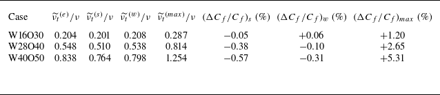

 HFχ
 HIχ
 Δk=|kz−s|
 Δc=2
 ks
 ks/2
 nkw(n=1,2,…)

 K
 ΠFχ(K)
 ΠIχ(K)
 Πnetχ(K)=ΠFχ(K)−ΠIχ(K)
 ks
 ks/2
 nkw(n=1,2,…)
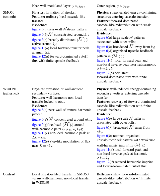
 N
 N^†
 ⟨M^†(kz,s)⟩Vχ
 Hqχ(Δk)
 Πqχ(K)
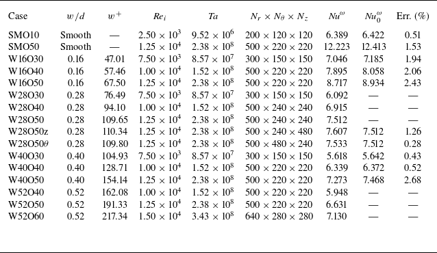
 Nu0ω
 θ
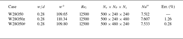
 θ

 θ
 Pθz
 Prθ



