1. Introduction
In a recent experimental investigation, where high-resolution infrared imagery was used to observe the flow over Space Shuttle Endeavour during its final re-entry, Horvath et al. (Reference Horvath, Zalameda, Wood and Berry2012) have shown that laminar–turbulent transition in typical high-speed flight situations is dominated by the effects of roughness elements. The observations were carried out over a range of Mach numbers between 6 and 18 and clearly showed the occurrence of wedge-like patches of high wall temperature caused by the laminar–turbulent transition induced by imperfections in the Space Shuttle’s fuselage. These observations are in agreement with wind tunnel experiments, which have consistently shown that localised or distributed roughness can lead to a significant acceleration of the laminar–turbulent transition process at low and high speeds (Tani & Sato Reference Tani and Sato1956; Klebanoff & Tidstrom Reference Klebanoff and Tidstrom1972; Corke, Bar-Server & Morkovin Reference Corke, Bar-Server and Morkovin1986; Fujii Reference Fujii2006; Schneider Reference Schneider2008a ).
Experiments on the stability of subsonic boundary layers carried out by Klebanoff & Tidstrom (Reference Klebanoff and Tidstrom1972) showed that discrete two-dimensional roughness elements induce basic flow modifications which may lead to an enhanced growth of Tollmien–Schlicting (TS) waves, thereby leading to an early transition to turbulence. The effects of two-dimensional roughness elements on the stability of supersonic boundary layers were investigated by Marxen, Iaccarino & Shaqfeh (Reference Marxen, Iaccarino and Shaqfeh2010) using numerical simulations of the Navier–Stokes equations. In this case, an acceleration of the laminar–turbulent transition process, which was triggered by a wall blowing and suction forcing placed upstream of the roughness element, was found to be the consequence of a sudden amplification of the boundary-layer instability modes near the roughness element. Localised and distributed roughness plays a crucial role on the receptivity (i.e. the conversion of external disturbances into the boundary-layer modes) of boundary layers subjected to free-stream disturbances. This is especially true at low speeds, where the wavelength of the free-stream disturbances is much greater than that of the TS waves and the roughness provides the wavelength conversion mechanism required for the excitation of the boundary-layer instabilities (Kachanov, Kozlov & Levchenko Reference Kachanov, Kozlov and Levchenko1979; Ruban Reference Ruban1984; Goldstein Reference Goldstein1985; Choudhari & Street Reference Choudhari and Street1992; Crouch Reference Crouch1992; Wu Reference Wu2001). On the other hand, three-dimensional roughness elements with heights comparable to the local boundary-layer thickness have much more profound effects on the boundary-layer flow and often lead to a great acceleration of the laminar–turbulent transition process. Typically, such roughness elements tend to induce counter-rotating streamwise vortices (see for example Gaster, Grosch & Jackson Reference Gaster, Grosch and Jackson1994; Joslin & Grosch Reference Joslin and Grosch1995; Tumin & Reshotko Reference Tumin and Reshotko2005; Rizzetta & Visbal Reference Rizzetta and Visbal2007; Ruban & Kravtsova Reference Ruban and Kravtsova2013) which drive the transient growth of a low-velocity streak surrounded by regions of detached high shear in the roughness wake, where new instabilities may develop (Choudhari et al. Reference Choudhari, Li, Minwei, Chang and Edwards2010; Kegerise et al. Reference Kegerise, King, Owens, Choudhari, Li, Chang and Norris2012; De Tullio et al. Reference De Tullio, Paredes, Sandham and Theofilis2013). In addition, large three-dimensional roughness elements induce regions of separated flow where absolute instabilities may develop in ways that are currently not well understood (see for example Chang, Choudhari & Li Reference Chang, Choudhari and Li2010; Subbareddy, Bartkowicz & Candler Reference Subbareddy, Bartkowicz and Candler2014).
The lack of understanding of the numerous processes contributing to the roughness-induced transition to turbulence means that current roughness-induced transition prediction methodologies rely upon empirical correlations. These correlations are largely based on the concept of a critical roughness Reynolds number
 $\mathit{Re}_{h}$
, which is defined, for example, as
 $\mathit{Re}_{h}=u_{h}h/{\it\nu}_{h}$
where
 $u_{h}$
and
 ${\it\nu}_{h}$
are the streamwise velocity and kinematic viscosity taken at
 $y=h$
in the corresponding clean flat plate boundary layer (other definitions can be found in Reda Reference Reda2002). The importance of the critical roughness Reynolds number approach for the prediction of roughness-induced transition was highlighted in the review work of Reda (Reference Reda2002). Recently Redford, Sandham & Roberts (Reference Redford, Sandham and Roberts2010) investigated the effects of discrete roughness elements on the laminar–turbulent transition occurring in supersonic flat-plate boundary layers using numerical simulations of the compressible Navier–Stokes equations. Their results suggest that transition to turbulence is dominated by roughness effects provided
 $\mathit{Re}_{h}$
exceeds a critical value which increases as the parameter
 $M_{h}T_{\infty }/T_{w}$
increases, where
 $M_{h}$
is the Mach number calculated at the roughness edge and
 $T_{w}$
is the wall temperature, starting from
 $\mathit{Re}_{h}=300$
at
 $M_{h}T_{\infty }/T_{w}=0$
. This criterion was later modified by Bernardini et al. (Reference Bernardini, Pirozzoli, Orlandi and Lele2014) to include the the effects of roughness shape through the introduction of a Reynolds number based on the momentum deficit between the upstream undisturbed boundary-layer flow and the roughness wake. An alternative model based on a transient growth mechanism was proposed by Reshotko & Tumin (Reference Reshotko and Tumin2004).
Recognising the important role played by roughness wakes on the roughness-induced transition, a number of researchers have concentrated their efforts on studying the stability characteristics of the wakes induced by roughness elements of different sizes and shapes and under different flow conditions (Choudhari et al.
Reference Choudhari, Li, Minwei, Chang and Edwards2010; Kegerise, Owens & Rudolf Reference Kegerise, Owens and Rudolf2010; Owens, Kegerise & Wilkinson Reference Owens, Kegerise and Wilkinson2011; Kegerise et al.
Reference Kegerise, King, Owens, Choudhari, Li, Chang and Norris2012; Groskopf & Kloker Reference Groskopf and Kloker2012; De Tullio & Sandham Reference De Tullio and Sandham2012; Wheaton & Schneider Reference Wheaton and Schneider2012; Choudhari et al.
Reference Choudhari, Li, Chang, Norris and Edwards2013; De Tullio et al.
Reference De Tullio, Paredes, Sandham and Theofilis2013; Wheaton & Schneider Reference Wheaton and Schneider2013), using a combination of experiments, linear stability analysis (LST) and numerical simulations of the Navier–Stokes equations. The results indicate that the laminar–turbulent transition of the roughness wake occurs as a consequence of the growth of sinuous (i.e. with an antisymmetric
 $u$
-velocity eigenfunctions with respect to the roughness mid-plane) and/or varicose (i.e. with a symmetric
 $u$
-velocity eigenfunctions with respect to the roughness mid-plane) wake modes. These modes are due to the instability of the high-shear layers induced by the counter rotating vortex pair in the wake of the roughness element. The experimental and biglobal stability results presented by Choudhari et al. (Reference Choudhari, Li, Minwei, Chang and Edwards2010) and Kegerise et al. (Reference Kegerise, King, Owens, Choudhari, Li, Chang and Norris2012) for a diamond-shaped roughness elements at
 $M=3.5$
show that both sinuous and varicose modes can grow substantially in the linear stages of the transition process; for
 $\mathit{Re}_{h}=426$
the experiments show that the transition process is driven by the varicose mode, while the sinuous mode dominates for
 $\mathit{Re}_{h}=319$
. The amplitude functions obtained from their biglobal stability results were found to be in good qualitative agreement with the experimentally obtained mode shapes. The instability induced by discrete three-dimensional roughness elements in a
 $M=4.8$
boundary layer was studied by Groskopf, Kloker & Marxen (Reference Groskopf, Kloker, Marxen, Henningson and Schlatter2009) using biglobal stability and Navier–Stokes simulations. They also report good agreement between the modes shapes obtained using the two methodologies. De Tullio et al. (Reference De Tullio, Paredes, Sandham and Theofilis2013) analysed the laminar–turbulent transition induced by a sharp-edged roughness element in a boundary layer at
 $M=2.5$
using a combination of Navier–Stokes, spatial biglobal and three-dimensional parabolised stability (PSE-3D) results. In this case the wake instability is dominated by the varicose mode, which drives the flow all of the way to breakdown to turbulence. In line with previous studies, De Tullio et al. (Reference De Tullio, Paredes, Sandham and Theofilis2013) report good agreement between biglobal and Navier–Stokes results for the amplitude functions of the different wake modes. However, due to non-parallel flow effects, the biglobal stability analysis was typically out by 12 % in growth rates. These, on the other hand, were found to be correctly predicted using the PSE-3D methodology, which was found to be in excellent agreement with the Navier–Stokes simulations. Further experimental results demonstrating the importance of the roughness wake instability as the cause of the early laminar–turbulent transition observed in the presence of isolated roughness elements were reported by Kegerise et al. (Reference Kegerise, Owens and Rudolf2010) and Owens et al. (Reference Owens, Kegerise and Wilkinson2011). Recently Wheaton & Schneider (Reference Wheaton and Schneider2012, Reference Wheaton and Schneider2013) have carried out a set of experiments on roughness-induced transition at
 $M=6$
, reporting the first quantitative measurements of the roughness wake instability at hypersonic speeds.
The above and other research works (see for example Berry & Horvath Reference Berry and Horvath2008; Borg & Schneider Reference Borg and Schneider2008; Schneider Reference Schneider2008b
; Chang, Choudhari & Li Reference Chang, Choudhari and Li2011; Iyer & Mahesh Reference Iyer and Mahesh2013; Fiala, Hillier & Estruch-Samper Reference Fiala, Hillier and Estruch-Samper2014) have highlighted the important role played by roughness on the laminar–turbulent transition process, especially at high speeds. Although roughness-induced transition is far from being understood, it is now clear that roughness elements can favour the excitation of boundary-layer instabilities and induce highly unstable wakes, thereby introducing an additional path to turbulence which resembles the bypass transition scenario. However, to the best of the authors’ knowledge, there are no studies available in the literature on the sensitivity of the roughness wake to different disturbance environments, and hence an explanation of the possible mechanisms responsible for the excitation of the different wake modes is currently missing. This issue is considered in this paper, where the effects of different disturbance environments on the linear stability of the flow around a sharp-edge roughness element in a boundary layer at
 $M=6$
are investigated using numerical simulations of the Navier–Stokes equations. The remainder of the paper is organised as follows. In § 2 the dimensionless form of the compressible Navier–Stokes equations is presented, along with the numerical schemes used for their integration. All of the details of the numerical study are given in § 3. The results are discussed in § 4 and the paper ends in § 5, where the main conclusions of the present study are drawn.
2. Mathematical and numerical modelling
The investigation is carried out through the numerical solution of the compressible Navier–Stokes equations, which in dimensionless form can be written as
 $$\begin{eqnarray}\displaystyle & \displaystyle \frac{\partial {\it\rho}}{\partial t}+\frac{\partial {\it\rho}u_{j}}{\partial x_{j}}=0 & \displaystyle\end{eqnarray}$$
 $$\begin{eqnarray}\displaystyle & \displaystyle \frac{\partial {\it\rho}u_{i}}{\partial t}+\frac{\partial {\it\rho}u_{i}u_{j}}{\partial x_{j}}+\frac{\partial p}{\partial x_{i}}=\frac{\partial {\it\tau}_{ij}}{\partial x_{j}} & \displaystyle\end{eqnarray}$$
 $$\begin{eqnarray}\displaystyle & \displaystyle \frac{\partial {\it\rho}E}{\partial t}+\frac{\partial \left({\it\rho}E+p\right)u_{i}}{\partial x_{i}}=-\frac{\partial q_{i}}{\partial x_{i}}+\frac{\partial u_{i}{\it\tau}_{ij}}{\partial x_{j}}. & \displaystyle\end{eqnarray}$$
 ${\it\tau}_{ij}$
, is defined as
 $$\begin{eqnarray}{\it\tau}_{ij}=\frac{{\it\mu}}{\mathit{Re}}\left(\frac{\partial u_{j}}{\partial x_{i}}+\frac{\partial u_{i}}{\partial x_{j}}-\frac{2}{3}\frac{\partial u_{k}}{\partial x_{k}}{\it\delta}_{ij}\right),\end{eqnarray}$$
where
 ${\it\delta}_{ij}$
is the Kronecker delta function defined as
 ${\it\delta}_{ij}=1$
for
 $i=j$
and
 ${\it\delta}_{ij}=0$
for
 $i\neq j$
. The properties of the fluid and the components of the heat flux vector (
 $q_{j}$
) are calculated considering the equation of state and Fourier’s law of heat conduction, given respectively by
 $$\begin{eqnarray}p=({\it\gamma}-1)\left({\it\rho}E-\frac{1}{2}{\it\rho}u_{i}u_{i}\right)=\frac{1}{{\it\gamma}M^{2}}{\it\rho}T\quad \text{and}\quad q_{j}=-\frac{{\it\mu}}{({\it\gamma}-1)M^{2}\mathit{Pr}\mathit{Re}}\frac{\partial T}{\partial x_{j}}.\end{eqnarray}$$
The dynamic viscosity is calculated from the temperature field using the Sutherland’s law
 ${\it\mu}=T^{3/2}(1+S^{\ast }/T_{r}^{\ast })/(T+S^{\ast }/T_{r}^{\ast })$
, where
 $S^{\ast }=110.4~\text{K}$
is the Sutherland constant for air and
 $T_{\infty }^{\ast }=273.15~\text{K}$
. Dimensionless variables are obtained as
 $$\begin{eqnarray}t=\frac{t^{\ast }U_{\infty }}{{\it\delta}_{0}^{\ast }},\quad x_{i}=\frac{x_{i}^{\ast }}{{\it\delta}_{0}^{\ast }},\quad u_{i}=\frac{u_{i}^{\ast }}{U_{\infty }},\quad {\it\rho}=\frac{{\it\rho}^{\ast }}{{\it\rho}_{\infty }},\end{eqnarray}$$
 $$\begin{eqnarray}p=\frac{p^{\ast }}{{\it\rho}_{\infty }U_{\infty }^{2}},\quad {\it\mu}=\frac{{\it\mu}^{\ast }}{{\it\mu}_{\infty }},\quad E=\frac{E^{\ast }}{U_{\infty }^{2}},\end{eqnarray}$$
where asterisks (
 $\ast$
) denote dimensional quantities and
 ${\it\delta}_{0}^{\ast }$
is the displacement thickness of the laminar boundary layer at
 $x=-16$
, where
 $x=0$
is at the computational domain inflow (see figure 1). Here,
 $t^{\ast }$
is time,
 $(x_{1}^{\ast },x_{2}^{\ast },x_{3}^{\ast })=(x^{\ast },y^{\ast },z^{\ast })$
are the streamwise, wall-normal and spanwise components of the position vector on a reference frame placed at the computational domain inflow and on the roughness mid-plane,
 $(u_{1}^{\ast },u_{2}^{\ast },u_{3}^{\ast })=(u^{\ast },v^{\ast },w^{\ast })$
are the streamwise, wall-normal and spanwise components of the velocity vector,
 ${\it\rho}^{\ast }$
is the density,
 $p^{\ast }$
is the pressure,
 ${\it\mu}^{\ast }$
is the dynamic viscosity and
 $E^{\ast }$
is the total energy per unit mass. The dimensionless parameters which define the problem are the Reynolds number
 $\mathit{Re}_{{\it\delta}_{0}^{\ast }}={\it\rho}_{\infty }U_{\infty }{\it\delta}_{0}^{\ast }/{\it\mu}_{\infty }$
, the Mach number
 $M$
and the Prandtl number
 $\mathit{Pr}=0.72$
. Noting that
 $$\begin{eqnarray}\mathit{Re}_{\tilde{x}^{\ast }}=\frac{1}{2}\left(\frac{\mathit{Re}_{{\it\delta}_{0}^{\ast }}}{{\it\Delta}}\right)^{2}+\mathit{Re}_{{\it\delta}_{0}^{\ast }}x,\end{eqnarray}$$
where
 $\tilde{x}^{\ast }$
is the dimensional distance from the flat-plate leading edge and
 ${\it\Delta}$
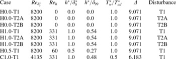
is a scaling factor obtained from the compressible similarity solution (given in table 1 for the different cases considered), the dimensionless simulation data can be converted to a reference system based on the flat-plate that would be used in an experiment (for more details see De Tullio et al. (Reference De Tullio, Paredes, Sandham and Theofilis2013)).
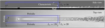
Computational domain and boundary conditions, sketched over grey contours of temperature obtained from a separate direct numerical simulation (De Tullio Reference De Tullio2013) of roughness-induced transition to turbulence at
 $M=6$
. In the present work the coordinate system is fixed to a smaller domain as shown, with boundary conditions as labelled (Extrap. denoting an inflow condition using an extrapolation of pressure).

Details of the computational study.

The compressible Navier–Stokes equations (2.1a )–(2.1c ) are solved numerically using high-order finite differences. The spatial discretisation is treated using a standard fourth-order central difference scheme to calculate derivatives at internal points, while close to boundaries a stable boundary treatment by Carpenter, Nordstrom & Gottlieb (Reference Carpenter, Nordstrom and Gottlieb1999) is applied, giving overall fourth-order accuracy. Time integration is based on a third-order compact Runge–Kutta method (Wray Reference Wray1990) and an entropy splitting approach (Sandham, Li & Yee Reference Sandham, Li and Yee2002) is used to split the inviscid flux derivatives into conservative and non-conservative parts, thereby improving numerical stability. The code has multi-block capabilities and is made parallel (both intra- and inter-block) using the Message Passing Interface (MPI) library. Details on the implementation of the numerical schemes can be found in Li (Reference Li2003) and Jones (Reference Jones2008). The multi-block version of the code used in this work was validated extensively (see for example De Tullio & Sandham Reference De Tullio and Sandham2010; De Tullio et al. Reference De Tullio, Paredes, Sandham and Theofilis2013).
3. Details of the numerical study
Figure 1 shows an example of roughness-induced transition to turbulence in a boundary layer at
 $M=6$
(obtained from a separate direct numerical simulation study, the details of which can be found in De Tullio & Sandham (Reference De Tullio and Sandham2012)), where the roughness element leads to a noticeable acceleration of the laminar–turbulent transition process in the presence of small external perturbations, while failing to introduce unstable global modes into the system. It can be clearly seen that the wake of the roughness element becomes unstable, breaks down into turbulence and leads to the generation of a turbulent wedge downstream of the roughness element. The aim of the present study is to shed some light into the mechanisms driving the linear wake instability, prior to the nonlinear breakdown to turbulence, and, in particular, how these may be affected by different disturbances developing in the boundary layer.
3.1. Numerical simulations
The main part of the investigation focuses on a roughness element with a dimensionless height
 $h=1.0$
, corresponding to a dimensional height of
 $h^{\ast }=0.54\times {\it\delta}_{99}$
, where
 ${\it\delta}_{99}$
is the local boundary-layer thickness. The numerical simulations for the reference configuration were carried out for
 $M=6$
,
 $\mathit{Re}_{{\it\delta}_{0}^{\ast }}=8200$
and for a constant wall temperature
 $T_{w}^{\ast }$
equal to the laminar adiabatic wall temperature
 $T_{ad}^{\ast }$
, hence
 $$\begin{eqnarray}T_{w}=1+\mathit{Pr}^{1/2}\frac{{\it\gamma}-1}{2}M^{2}.\end{eqnarray}$$
Under these conditions the roughness Reynolds number is
 $\mathit{Re}_{h}=331$
, which was selected to lie just below the critical
 $\mathit{Re}_{h}$
proposed by Redford et al. (Reference Redford, Sandham and Roberts2010). In a recent numerical investigation, Van den Eynde & Sandham (Reference Van den Eynde and Sandham2014) have shown that sharp-edged roughness elements (such as those considered in this work) are more effective at promoting laminar–turbulent transition than the smooth bumps used in the work of Redford et al. (Reference Redford, Sandham and Roberts2010). Therefore, it is reasonable to expect that the current simulations are in a flow regime where the disturbance environment is critically important in determining whether a given flow undergoes transition to turbulence.
In order to explore the effects of varying roughness height, a roughness element with dimensionless height
 $h=0.5$
is also considered, which, keeping the same Mach and Reynolds numbers as for the reference configuration, leads to
 $\mathit{Re}_{h}=60$
. An additional simulation is also carried out for a wall temperature of
 $T_{w}^{\ast }=0.5\times T_{ad}^{\ast }$
in order to analyse the effects of wall cooling on the stability of the wake, where the roughness Reynolds number is kept the same as for the reference configuration in order to minimise local Reynolds number effects. In all of the cases the roughness element has the shape of a rectangular parallelepiped, with length
 $L_{r}=6.0$
and width
 $W_{r}=6.0$
, having one of its sides perpendicular to the incoming flow. For a direct comparison between the boundary-layer instability and the roughness-induced instability, additional numerical simulations for a smooth flat plate were also carried out.
The steady basic flows obtained for the above configurations are perturbed by artificial disturbances introduced at the inflow of the computational domain. The analysis is carried out for three different types of inflow perturbations, referred to here as T1, T2A and T2B, which are given by
 $$\begin{eqnarray}\displaystyle & \text{T1}\rightarrow {\it\rho}(x_{0},y,z,t)={\it\rho}_{b}(x_{0},y,z)+{\it\psi}(y,z,t), & \displaystyle\end{eqnarray}$$
 $$\begin{eqnarray}\displaystyle & \text{T2A, T2B}\rightarrow \left\{\begin{array}{@{}l@{}}v(x_{0},y,z,t)=v_{b}(x_{0},y,z)-\partial {\it\psi}(y,z,t)/\partial z\quad \\ w(x_{0},y,z,t)=w_{b}(x_{0},y,z)+\partial {\it\psi}(y,z,t)/\partial y,\quad \end{array}\right. & \displaystyle\end{eqnarray}$$
 $$\begin{eqnarray}{\it\psi}(y,z,t)=aG(y)\mathop{\sum }_{m=0}^{M-1}\mathop{\sum }_{n=1}^{N}\cos ({\it\beta}_{m}z+{\it\phi}_{m})\cos ({\it\omega}_{n}t+{\it\psi}_{n}),\end{eqnarray}$$
with
 $N=16$
and
 $M=7$
as the number of frequencies and spanwise wavenumbers, respectively,
 ${\it\beta}_{m}=m2{\rm\pi}/Lz$
,
 ${\it\omega}_{n}=n2{\rm\pi}F_{0}$
with
 $F_{0}=0.02$
(note that in all cases the forcing function contains a
 ${\it\beta}=0$
spanwise mode). The forced frequencies were selected to sample the range of most unstable frequencies in the wake of the roughness element. Note that the non-dimensional frequency
 $F=f^{\ast }{\it\delta}_{0}^{\ast }/U_{\infty }^{\ast }$
,
 $f^{\ast }$
being the dimensional frequency (cycles per second), takes the form of a Strouhal number; the standard frequency definition
 $F_{s}=2{\rm\pi}f^{\ast }{\it\mu}_{\infty }^{\ast }/({\it\rho}_{\infty }^{\ast }{U_{\infty }^{\ast }}^{2})$
used in linear stability studies can be recovered from
 $F_{s}=2{\rm\pi}F/\mathit{Re}_{{\it\delta}_{0}^{\ast }}$
. The phases
 ${\it\phi}_{m}$
and
 ${\it\psi}_{n}$
are set to random numbers between 0 and
 $2{\rm\pi}$
in order to avoid local peaks in the disturbance signal which might trigger undesired nonlinearities. T2A and T2B perturbations differ in the form of the damping function
 $G$
, which is used to take the disturbances to zero at the flat plate wall. The damping function is defined as
 $$\begin{eqnarray}\displaystyle & G(y)=1-\text{e}^{-y^{3}}\quad \text{for T1 and T2A}, & \displaystyle\end{eqnarray}$$
 $$\begin{eqnarray}\displaystyle & G(y)=1-\text{e}^{-y^{12}/(2^{22})}\quad \text{for T2B}, & \displaystyle\end{eqnarray}$$
 $a=2\times 10^{-6}$
is used to ensure the linearity of the dominating transition mechanisms. It should be noted that, while being divergence free, in practise T2A and T2B perturbations also introduce acoustic waves into the computational domain (as will be shown in § 4.1), the effect of which will be discussed in § 4.3.
The inflow perturbations were designed to obtain three fundamentally different disturbance fields inside the boundary layer. In particular, as will be shown in § 4.1, T1 perturbations induce a disturbance field dominated by two-dimensional boundary-layer modes (first modes and Mack modes), the disturbances induced by T2A perturbations include oblique first modes and Mack modes but no two-dimensional modes, while in the case of T2B perturbations the boundary-layer disturbances are dominated by the fast acoustic waves travelling obliquely (i.e. with
 ${\it\beta}\neq 0$
) to the flow direction. Note that our approach differs from that used in other computational studies (see for example Jacobs & Durbin Reference Jacobs and Durbin2001; Brandt, Schlatter & Henningson Reference Brandt, Schlatter and Henningson2004), where a synthetic turbulent inflow is used to model the effects of free-stream turbulence on the boundary-layer laminar–turbulent transition. Here, we are interested in the excitation of the roughness wake instabilities for different boundary-layer disturbance fields (and our inflow disturbances are tailored for this type of analysis), rather than on the receptivity of the boundary-layer upstream of the roughness element.
All of the relevant details of the numerical simulations reported in this work are shown in table 1, where the simulations are named with a prefix indicating the wall temperature (H for
 $T_{w}^{\ast }=T_{ad}^{\ast }$
and C for
 $T_{w}^{\ast }=0.5\times T_{ad}^{\ast }$
), followed by the height of the roughness element, and a suffix indicating the type of inflow perturbations considered.
3.2. Computational domain and boundary conditions
As indicated in figure 1, the computational domain used for the numerical simulations has dimensions
 $L_{x}\times L_{y}\times L_{z}=150\times 16\times 20$
and does not include the flat plate leading edge and its associated shock. The computational inflow is initialised with a compressible laminar similarity solution and a pressure extrapolation boundary condition, whereby in the subsonic region of the boundary layer the inflow conservative variables are calculated by linearly extrapolating the pressure from within the domain, is used for the calculation of the steady laminar base flows. The reflection of waves from the top and outflow boundaries is minimised by using integrated and standard characteristic conditions, respectively. The standard characteristic conditions used here are those originally derived by Thompson (Reference Thompson1987, Reference Thompson1990), whereby the rates of change of incoming characteristics are set to zero at characteristic boundaries. A periodic boundary condition is applied at the spanwise domain boundaries and the flat-plate wall is considered no-slip and isothermal. It should be noted that the application of an isothermal wall boundary condition means that the effects of wall temperature variations due to the wall heat transfer are neglected. The same applies to laboratory experiments of high-speed laminar–turbulent transition, where, unlike in typical flight situations, the short duration of the tests does not allow time for significant changes in wall temperature. Therefore, the flow conditions considered in this work are closer to those typical of laboratory experiments than to those typically occurring during flight.
The streamwise extent of the computational domain was chosen to obtain a significant linear growth of the most unstable disturbances, while the wall normal domain size was designed so that any residual reflections coming from the top boundary (i.e. the weak shocks generated upstream and downstream of the roughness element, see later) would hit the outflow boundary without affecting the flow downstream of the roughness element. The periodic boundary condition used for the spanwise domain boundaries means that the simulations are effectively for a spanwise periodic array of roughness elements. Since the most unstable Mack modes at
 $M=6$
are two-dimensional, the spanwise extent of the computational domain was chosen large enough to keep the roughness element from interacting with its spanwise neighbours, while still keeping the numerical simulations to a manageable size.
All of the numerical grids were stretched in the wall-normal direction using the following relation between the computational uniform grid (
 $0<{\it\eta}<1$
) and the physical non-uniform grid (
 $0<y<L_{y}$
)
 $$\begin{eqnarray}y=L_{y}\frac{\sinh (b_{y}{\it\eta})}{\sinh b_{y}},\end{eqnarray}$$
where
 $b_{y}$
is the stretching factor, given in table 2. In the cases including a roughness element the value of
 $b_{y}$
was iteratively determined (close to a target) by imposing an integer number of grid points (
 $n_{y}^{r}$
) below the roughness and
 $y(n_{y}^{r})=h$
, where
 $h$
is the non-dimensional height of the roughness element. The distribution of grid points in the streamwise and spanwise directions is uniform in the cases involving clean flat plates, whereas for the cases including roughness elements it was designed to adequately resolve the laminar flow near the roughness element and the instabilities developing in its wake. Grid points were clustered near the roughness element so that the resulting grid is stretched in all directions. In the horizontal directions (
 $x$
and
 $z$
) the computational grid presents regions of constant grid spacing with different levels of grid refinement. These regions are linked together by polynomials of the ninth degree obtained by imposing
 $C^{4}$
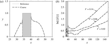
continuity of the resulting stretching function. Details of the numerical grids employed in each case are provided in table 2. The grids were chosen after a grid-convergence study which showed negligible variations for the growth of disturbances when considering a grid with half the number of points in all directions. The effects of grid refinement on the base flow and the stability of the roughness wake for case H1.0-T1 are shown in figure 2(a,b), respectively. It can be seen that the differences between the results obtained with the reference and the coarse grids are negligible.
Computational grids. Here
 $N_{x}$
,
 $N_{y}$
and
 $N_{z}$
are the number of points in the streamwise, wall-normal and spanwise directions, while
 $n_{y}^{r}$
is the number of points for
 $0\leqslant y\leqslant h$
. The length and width of the roughness elements are resolved using
 $n_{x}^{r}=101$
and
 $n_{z}^{r}=121$
points, respectively, in all cases.

Grid convergence study. (a) Contours of small negative basic flow
 $u$
-velocity showing the roughness-induced separation bubbles at the roughness centreline (note that the
 $y$
-axis has been stretched for clarity). (b) Amplitude of the
 $v$
-velocity boundary-layer disturbances, defined as in (4.5), for a selection of unstable frequencies. The shaded grey areas indicate the roughness element position.

4. Results
4.1. Disturbances excited inside the smooth flat plate boundary layer
The evolution of disturbances in the boundary layer developing over a smooth flat plate is analysed in this section in order to characterise the disturbance environments associated with the three types of inflow perturbations considered. Attention will be focused on the hot-wall case (case prefix H0.0) as it represents the reference case for the present study. In order to put things into perspective, we start by reporting the results of a spatial LST of the flow.
According to LST, the critical Reynolds number above which two-dimensional (
 $m=0$
) Mack modes first become unstable for the flow conditions considered is
 $\mathit{Re}_{x_{crit}^{\ast }}\approx 4.5\times 10^{4}$
. The computational domain used for the numerical simulations is such that the inflow and outflow Reynolds numbers are
 $\mathit{Re}_{x_{in}^{\ast }}\approx 5.4\times 10^{5}$
and
 $\mathit{Re}_{x_{out}^{\ast }}\approx 17.7\times 10^{5}$
, thereby enclosing a region of the boundary layer where first modes and Mack modes are both unstable. For the Mack number considered here, the most unstable boundary-layer modes are two-dimensional Mack modes, while the most unstable first modes are oblique (
 $m\neq 0$
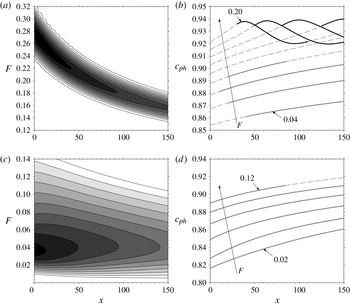
). Figure 3(a) shows the linear spatial stability diagram for the
 $m=0$
Mack mode, where contours of the modes growth rates are plotted as a function of frequency (
 $F$
) and streamwise distance (
 $x$
) inside the computational domain. The most unstable Mack modes included in the computational domain have growth rates ranging from
 $-{\it\alpha}_{i}=0.0282$
for
 $F=0.28$
at the computational domain inflow to
 $-{\it\alpha}_{i}=0.0196$
for
 $F=0.16$
at the outflow. Mack modes can reach growth rates as high as
 $-{\it\alpha}_{i}\approx 0.032$
at
 $\mathit{Re}_{x^{\ast }}\approx 1.71\times 10^{5}$
(i.e. upstream of the computational domain inflow) for
 $F=0.48$
. Note, however, that the length of the region of Mack mode instability decreases sharply as the distance from the flat plate leading edge is decreased. Considering a trade off between peak growth rate and extent of the region of instability the
 $F=0.18$
Mack mode may be regarded as one of the most dangerous instabilities for the boundary layer considered here. This mode has a maximum growth rate of
 $-{\it\alpha}_{i}=0.0223$
at
 $x=95~(\mathit{Re}_{x^{\ast }}\approx 13.6\times 10^{5})$
and its region of instability goes from
 $x\approx 47~(\mathit{Re}_{x^{\ast }}\approx 9.25\times 10^{5})$
to
 $x\approx 156~(\mathit{Re}_{x^{\ast }}\approx 18.2\times 10^{5})$
. Figure 3(b) gives the phase speeds of two-dimensional waves as a function of streamwise distance, for a selection of the most relevant frequencies. The figure also shows the regions of instability of two-dimensional first modes and Mack modes, shown respectively by the solid light grey and black lines. In addition to the unstable Mack modes, weakly unstable two-dimensional first modes are obtained for
 $0.04\leqslant F<0.12$
. The phase speeds of the first modes range from
 $c_{ph}\approx 0.86$
for
 $F=0.04$
to
 $c_{ph}\approx 0.90$
for
 $F=0.10$
, while those of the unstable Mack modes vary in the streamwise direction from
 $c_{ph}\approx 0.94$
to
 $c_{ph}\approx 0.92$
irrespective of the frequency.
Spatial LST of the smooth flat-plate boundary layer: (a) spatial stability diagram
 $-{\it\alpha}_{i}=f(x,F)$
for two-dimensional (
 $m=0$
) Mack modes, showing 10 equally spaced contours from 0.001 to 0.025; (b) phase speed as a function of streamwise distance for two-dimensional (
 $m=0$
) waves and for a selection of frequencies, the light grey and black solid lines show the regions of instability of first modes and Mack modes, respectively; (c) spatial stability diagram
 $-{\it\alpha}_{i}=f(x,F)$
for
 $m=2$
first modes, showing 10 equally spaced contours from 0.0001 to 0.009; (d) phase speed as a function of streamwise distance for
 $m=2$
first modes and for a selection of frequencies, the light grey solid lines show the regions of instability.

Figure 3(c,d) show, respectively, the spatial stability diagram and the evolution of phase speeds as a function of streamwise distance for
 $m=2$
first modes. First mode growth rates are substantially lower than Mack mode ones for the Mach number considered. According to LST the most unstable resolved first mode has a growth rate varying from
 $-{\it\alpha}_{i}=0.0093$
at the inflow to
 $-{\it\alpha}_{i}=0.0059$
at the outflow for
 $F=0.04$
and
 $m=2$
, while an absolute maximum growth rate of
 $-{\it\alpha}_{i}=0.0112$
is obtained at
 $\mathit{Re}_{x^{\ast }}\approx 2.12\times 10^{5}$
for
 $F=0.07$
and
 $k_{z}=1.1$
. The phase speeds of the
 $m=2$
first modes vary from
 $c_{ph}\approx 0.82$
for
 $F=0.02$
to
 $c_{ph}\approx 0.91$
for
 $F=0.12$
.
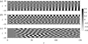
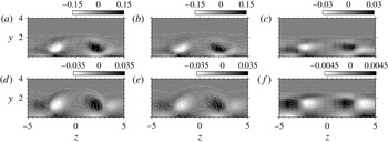
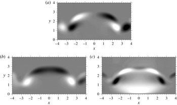
An example of the boundary-layer disturbances excited by the three types of inflow perturbations is shown in figure 4, which gives the real part of the Fourier-transformed (in time) wall pressure for
 $F=0.14$
. The figure is representative of the behaviour observed for all of the frequencies considered. The boundary-layer disturbance field associated with T1 perturbations is dominated by two-dimensional (
 $m=0$
) first modes and Mack modes for all of the frequencies considered. Figure 4(a) gives the disturbance field associated with T1 perturbations for
 $F=0.14$
, showing the development of a two-dimensional Mack mode which becomes unstable starting from
 $x\approx 110$
. Despite oblique first modes being more unstable than two-dimensional ones for the flow regime analysed here, the latter are dominant in the case of T1 perturbations because they are excited to a high initial amplitude by the inflow forcing.
Visualisation of the
 $F=0.14$
disturbances inside the boundary layer. Contours of the real part of the Fourier transformed wall pressure, normalised by the maximum value attained in the plane shown: (a) case H0.0-T1, (b) case H0.0-T2A and (c) case H0.0-T2B.

Figure 4(b) shows an example of the boundary-layer disturbances associated with T2A perturbations. In this case the inflow perturbations lead to the excitation of oblique first modes and Mack modes. The disturbance field is fully three-dimensional (for example in the region of flow for
 $z>4$
the flowfield shows a superposition of equal and opposite oblique modes), with its first (
 $m=0$
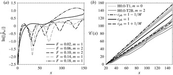
) spanwise Fourier coefficient more than two orders of magnitudes lower than the rest of the coefficients, and is given by a combination of boundary-layer modes and acoustic waves. This can be inferred from figure 5(a), which shows the streamwise evolution of the amplitude of the dominant wall pressure Fourier coefficients calculated using (4.3) for case H0.0-T2A. The periodic beating evident for some of the frequencies indicates that multiple modes with different phase speeds contribute to the wall pressure signal. Assuming that, for a certain frequency F, there are two modes at play with positive phase speeds
 $c_{ph}^{a}$
and
 $c_{ph}^{b}$
, it is easily shown that the following holds
 $$\begin{eqnarray}{\rm\Delta}x=\frac{c_{ph}^{a}c_{ph}^{b}}{F|c_{ph}^{a}-c_{ph}^{b}|},\end{eqnarray}$$
where
 ${\rm\Delta}x$
is the period of the beating. The periodic beating shown in figure 5(a) is consistent with the presence of boundary-layer modes with
 $c_{ph}\approx 0.88{-}0.94$
and fast acoustic waves with
 $c_{ph}\approx 1.1667$
. Note also that, as the boundary-layer modes grow, the amplitude of the beating decreases, as for example is evident for the case of an unstable
 $m=1$
Mack mode at
 $F=0.14$
. The amplitude of the periodic beating observed for the different Fourier coefficients indicates that, in general, the amplitudes of the boundary-layer modes and the acoustic waves near the wall are comparable, the former being slightly higher.
Characterisation of the boundary-layer disturbance environment: (a) streamwise evolution of the amplitude of the dominant wall-pressure Fourier coefficients calculated using (4.3) for case H0.0-T2; (b) phase speed of the dominant near-wall disturbances shown through
 $\mathscr{C}(x)={\it\phi}(x)/{\it\omega}$
, where the phases
 ${\it\phi}$
are obtained using (4.3) with the wall pressure. Each dark and light grey line corresponds a different forcing frequency.

Similarly to the case of T2A perturbations, the boundary-layer disturbance field associated with T2B perturbations is fully three-dimensional, as can be inferred from figure 4(c). However, in this case the disturbance field is given by the disturbances induced by a combination of fast acoustic waves propagating obliquely to the free-stream flow direction, which are the dominant waves inside the boundary layer. This is inferred from figure 5(b), which shows the streamwise evolution of
 $\mathscr{C}(x)={\it\phi}(x)/{\it\omega}=x/c_{ph}$
, where
 ${\it\phi}$
is the phase of the Fourier coefficients obtained using (4.3) for the wall pressure. Here,
 $\mathscr{C}(x)$
is used instead of
 $c_{ph}$
in order to avoid differentiation. Note that, while the phase speeds obtained in the case of T1 perturbations (light grey lines) coincide with those of the dominant boundary layer modes (which in turn are close to the phase speed of the free-stream slow acoustic waves), in the case of T2B perturbations (dark grey lines) they are close to the phase speed of the free stream fast acoustic waves. The observation that the long-wavelength fast acoustic waves dominate the boundary-layer disturbance field in the absence of boundary layer modes is consistent with the well-known shear sheltering mechanism (Hunt & Durbin Reference Hunt and Durbin1999). It should also be noted that the streamwise evolution of
 $\mathscr{C}(x)$
for case H0.0-T2A (not shown) agrees closely with that obtained for case H0.0-T1, which further indicates that the near-wall amplitudes of the boundary-layer modes are higher than those of the acoustic waves in this case.
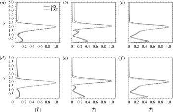
Finally, the amplitude functions of a selection of the dominant boundary-layer modes excited in cases H0.0-T1 and H0.0-T2A are compared with LST eigenfunctions of first modes and Mack modes in figure 6. Figure 6(a–c) show, respectively, the
 $m=0$
amplitude functions obtained for
 $F=0.06$
,
 $F=0.14$
and
 $F=0.18$
in the case of T1 perturbations. According to LST, the
 $F=0.06$
mode is a weakly unstable first mode that reaches a maximum growth rate of
 $-{\it\alpha}_{i}=0.00115$
, while the
 $F=0.14$
and
 $F=0.18$
modes are Mack modes with maximum growth rates of
 $-{\it\alpha}_{i}=0.0188$
and
 $-{\it\alpha}_{i}=0.0223$
, respectively. Figure 6(d–f) give, respectively, the
 $m=2$
amplitude function obtained for
 $F=0.06$
and the
 $m=1$
amplitude functions obtained for
 $F=0.14$
and
 $F=0.18$
in the case of T2A perturbations. The
 $F=0.06$
mode is an oblique first mode with maximum growth rate
 $-{\it\alpha}_{i}\approx 0.00765$
, while the modes obtained for
 $F=0.14$
and
 $F=0.18$
are oblique Mack modes with maximum growth rates
 $-{\it\alpha}_{i}\approx 0.0151$
and
 $-{\it\alpha}_{i}\approx 0.0193$
, respectively.
Comparison between the amplitude functions of the dominant disturbances obtained for a selection of frequencies and the corresponding LST eigenfunctions at
 $x=120$
: (a)
 $F=0.06$
and
 $m=0$
for case H0.0-T1; (b)
 $F=0.14$
and
 $m=0$
for case H0.0-T1; (c)
 $F=0.18$
and
 $m=0$
for case H0.0-T1; (d)
 $F=0.06$
and
 $m=2$
for case H0.0-T2A; (e)
 $F=0.14$
and
 $m=1$
for case H0.0-T2A; and ( f)
 $F=0.18$
and
 $m=1$
for case H0.0-T2A.

4.2. The laminar basic flow
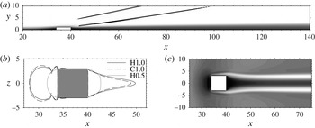
The laminar basic flows were obtained by simply integrating (2.1) without inflow forcing. This is possible because all of the flows considered in this work are only convectively unstable; i.e. all initial disturbances leave the computational domain after a certain transient. A general overview of the laminar basic flow around the roughness element is given in figure 7. The roughness element induces two regions of separated flow; a separation bubble upstream of its leading edge and one downstream of its trailing edge. The flow displacement caused by the flow separation and subsequent reattachment leads to the generation of a compression wave near the upstream separation point, followed by an expansion as the flow turns over the top of the roughness element and a further compression upon reattachment downstream. In all of the configurations analysed the downstream compression fan merges into a weak oblique shock. On the other hand, the upstream compression is weaker than the downstream one and a shock only forms for case C1.0, for which the Mach number near the edge of the roughness element is higher than for the rest of the cases. The upstream and downstream oblique shocks are shown in figure 7(a) by contours of
 $\boldsymbol{{\rm\nabla}}\boldsymbol{\cdot }u=-0.12$
(black line).
Main features of the basic flow over the roughness element. (a) Contours of
 $\boldsymbol{{\rm\nabla}}\boldsymbol{\cdot }u=-0.12$
(black line) showing the roughness-induced oblique shocks, superimposed over shaded contours of
 $u$
in a
 $x{-}y$
plane through the roughness centreline for case C1.0. (b) Contours of
 $u=0$
on a horizontal plane at the first grid point above the flat plate wall for the different cases considered, showing the upstream and downstream separation bubbles. (c) Contours of
 $u$
-velocity in a horizontal plane at
 $y=0.5$
.

Figure 7(b) gives a comparison of the separation bubbles induced by the roughness element in the three cases considered, which are visualised by contours of
 $u=0$
on a horizontal plane at the first grid point above the flat plate wall. A roughness element with height
 $h^{\ast }=0.27\times {\it\delta}_{99}$
(case H0.5) generates small separation bubbles upstream and downstream of the roughness element with similar size. As expected the size of the separation bubble increases as the roughness height is increased. The small differences in the separation bubbles obtained for cases H1.0 and C1.0 indicate that the effects of wall cooling on the flow near the roughness element are weak, the most notable effect being the slight shortening of the downstream bubble. The pinched shape of the upstream separation bubbles obtained for cases H1.0 and C1.0 is due to the presence of a pair of co-rotating horseshoe vortices, which wrap around the roughness element and quickly decay further downstream. In addition to these vortices a pair of counter-rotating streamwise vortices is also generated due to a small pressure difference between the top (higher) and the sides (lower) of the roughness element, as can be inferred from the development of a low-velocity streak near the roughness mid-plane, with two high-velocity streaks on its sides, shown in figure 7(b). These vortices influence both the size and shape of the downstream separation bubble. In fact, the slight shortening of the downstream separation bubble reported for case C1.0 is linked to the fact that, as will be shown later, the intensity of the counter-rotating vortex pair found for case C1.0 is lower than that obtained for case H1.0.
Regions of separated flow can potentially sustain the growth of absolute instabilities. However, in all of the configurations considered here the roughness element remains subcritical, meaning that it does not introduce unstable global modes. Nevertheless the counter-rotating vortex pair generated at the edges of the roughness element induces flow modifications in the downstream flow which, in some cases, are able to sustain the growth of additional convective instabilities. Figure 8 shows the basic flow in the wake of the roughness elements by plotting contours of
 $u$
-velocity, equally spaced between 0 and 1, superimposed with shaded contours of streamwise vorticity in
 $y{-}z$
planes at different
 $x$
-positions. It can be seen that in the large roughness cases H1.0 and C1.0, shown in figure 8(a–d), respectively, the counter-rotating vortex pair distorts the boundary-layer flow downstream of the roughness element. By lifting up low momentum fluid from the wall near the roughness mid-plane and pulling down high-momentum fluid from the free stream near the sides of the roughness element, the vortices generate a three-dimensional detached layer of high shear that surrounds the wake of the roughness element. The intensity of the counter-rotating vortex pair is highest for case H1.0 and only slightly lower for case C1.0, leading to slight differences in the wake flow for the two cases. Notice also that, as expected, wall cooling leads to the thickening of the boundary layer and that for cases H1.0 and C1.0 the shape of the roughness wake varies notably along the
 $x$
direction, suggesting that non-parallel flow effects should be taken into account when studying the excitation and subsequent development of wake instabilities. Figure 8(e,f) show the laminar flow downstream of the roughness element for case H0.5. It can be seen that by reducing the height of the roughness element by a factor of two, the boundary layer response changes drastically; the counter-rotating streamwise vortices become much weaker and introduce only marginal modifications to the boundary-layer flow downstream of the roughness element.
The structure of the roughness wake shown through contours of basic flow
 $u$
-velocity equally spaced between 0 and 1, superimposed over shaded contours of streamwise vorticity
 ${\it\omega}_{x}$
in
 $y{-}z$
planes at
 $x=60$
(a–c) and
 $x=120$
(d–f): (a,d) case H1.0; (b,e) case C1.0; and (c,f) case H0.5.

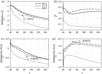
Figure 9 gives more quantitative comparisons between the wake flows obtained for the different configurations. The streamwise variation of the intensity of the counter-rotating vortex pair, measured here by the maximum streamwise vorticity attained over
 $y$
and
 $z$
, is shown in figure 9(a). Sufficiently far downstream of the roughness element the vortex pair intensity decreases exponentially in all cases, with the decay rate for cases H1.0 and C1.0 being
 ${\approx}{-}0.014$
. Despite continuously decaying, these vortices drive a low-velocity streak near the roughness mid-plane, the amplitude of which increases in the downstream direction. This is shown in figure 9(b), where the streak amplitude
 $A_{st}$
is defined as
 $$\begin{eqnarray}A_{st}=\max _{y}\left\{u_{b}(x,y,z_{0})-u_{b}(x,y,z_{m})\right\},\end{eqnarray}$$
where
 $z_{0}=-10$
and
 $z_{m}=0$
, hence at each
 $x$
-position the
 $u$
-velocity at the centre of the streak is compared with that in the surrounding boundary-layer flow. Note that the streak amplitude is higher for case C1.0 than for case H1.0, despite the intensity of the vortex pair being slightly lower. The streak amplitude decreases monotonically in the streamwise direction for case H0.5. As already anticipated, the vortex–streak system induces regions of detached high shear in the wake of the roughness element. The streamwise evolution of the maximum wall-normal and spanwise shear attained in the wake is shown in figure 9(c,d), respectively. In all cases the
 $\partial u/\partial y$
shear decreases monotonically for increasing
 $x$
, while the
 $\partial u/\partial z$
shear appears to increase algebraically initially and decrease exponentially further downstream, following a typical transient growth behaviour. Note that, sufficiently downstream of the roughness element, both the wall-normal and spanwise shear induced by the counter-rotating vortex pair for cases H1.0 and C1.0 decrease exponentially in the streamwise direction at a rate of
 ${\approx}{-}0.0033$
. The low decay rates observed for
 $A_{st}$
and the maximum
 $\partial u/\partial y$
and
 $\partial u/\partial z$
indicate that the wakes induced by roughness elements in these cases tend to persist for a long streamwise distance. This observation is in agreement with the results of a theoretical study recently performed by Ruban & Kravtsova (Reference Ruban and Kravtsova2013).
Quantitative comparisons between the wakes induced by the roughness elements in the different cases: (a) maximum streamwise vorticity inside the wake at each
 $y{-}z$
plane; (b) streak strength calculated as in (4.2); (c) maximum wall-normal basic flow shear inside the wake at each
 $y{-}z$
plane; and (d) maximum spanwise shear inside the wake at each
 $y{-}z$
plane.

4.3. Excitation of roughness-wake modes under different disturbance environments
In this section we analyse the response of the basic flow obtained for the reference case (case prefix H1.0) when subjected to the different disturbance environments discussed in § 4.1. The numerical results are analysed by decomposing the disturbance field into non-dimensional frequencies (
 $F$
) and spanwise wavenumbers (
 $k_{z}$
) using the following discrete Fourier transform formula
 $$\begin{eqnarray}\hat{{\hat{s}}}(x,y;{\it\eta},{\it\xi})=\frac{2}{LJ}\mathop{\sum }_{j=0}^{J-1}\mathop{\sum }_{l=0}^{L-1}s(x,y,z_{l},t_{j})\exp \left[-2{\rm\pi}\text{i}\frac{{\it\eta}}{J}j\right]\exp \left[-2{\rm\pi}\text{i}\frac{{\it\xi}}{L}l\right]\end{eqnarray}$$
where
 $J$
and
 $L$
are the total time and space samples and
 $s$
represents any flow variable. Here,
 ${\it\eta}$
and
 ${\it\xi}$
represent the discretised frequencies and spanwise wavenumbers, respectively. Non-dimensional frequencies can be obtained as
 $F={\it\eta}/{\it\tau}$
, with
 ${\it\eta}=0,1,\dots ,J/21$
, where
 ${\it\tau}=50$
is one sampling period (corresponding to one cycle at the lowest frequency of the forcing). The spanwise wavenumber spectrum can be reordered to have
 $k_{z}=2{\rm\pi}{\it\xi}/L_{z}$
, with
 ${\it\xi}=(L/21),\dots ,1,0,1,\dots ,L/21$
, where
 $L_{z}=20$
is the spanwise length of the computational domain. The normalisation factor
 $2/(LJ)$
gives unit amplitude Fourier modes for a disturbance signal given by a sum of temporal and spatial sinusoidal waves. The amplitude associated with each frequency is defined here as
 $$\begin{eqnarray}|{\hat{s}}|(x,y;{\it\eta})=\mathop{\sum }_{{\it\xi}=0}^{L-1}|\hat{{\hat{s}}}|(x,y;{\it\eta},{\it\xi})\end{eqnarray}$$
and the amplitude of the disturbances developing inside the boundary layer for each frequency is calculated as
 $$\begin{eqnarray}\langle |{\hat{s}}|\rangle (x;{\it\eta})=\int _{0}^{{\it\delta}_{99}}|{\hat{s}}|(x,y;{\it\eta})\text{d}y.\end{eqnarray}$$
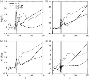
A comparison between the flow responses obtained for cases H1.0-T1, H1.0-T2A and H1.0-T2B is shown in figure 10 through the evolution of
 $v$
-velocity disturbances inside the boundary layer for a selection of frequencies. Note that the disturbance amplitudes are normalised with the values attained at
 $x=28$
(immediately upstream of the separation bubble in front of the roughness element) in all cases. At
 $F=0.02$
all of the cases show disturbances growing in the downstream direction at a rate of about
 $-{\it\alpha}_{i}=0.012$
(see figure 10
a for
 $x>120$
), indicating that the dominant instability is the same in all cases. As the forcing frequency is increased, the growth rates of the disturbances developing downstream of the roughness element increase in all cases. However, differences start appearing in the evolution of disturbances observed for the three different inflow perturbations. The responses obtained for
 $F=0.06$
, and given in figure 10(b), show clearly that the disturbances excited in the H1.0-T1 case grow considerably faster than those excited in cases H1.0-T2A and H1.0-T2B. At
 $F=0.06$
the disturbance growth rate reaches a local maximum of
 $-{\it\alpha}_{i}\approx 0.025$
for case H1.0-T1. In this case, as the frequency increases further the growth rate of the disturbances developing in the wake of the roughness element decreases, only to start increasing again from about
 $F=0.12$
, reaching a second local maximum of
 $-{\it\alpha}_{i}\approx 0.026$
at
 $F=0.14$
. The situation is different for case H1.0-T2B, where the disturbance growth rates increase up to an absolute maximum of
 $-{\it\alpha}_{i}\approx 0.0146$
at
 $F=0.08$
and decrease continuously thereafter. The variation of disturbance growth rates with frequency appears less straightforward for case H1.0-T2A. In this case, the disturbance amplification agrees with that observed in the H1.0-T1 case for some frequencies (i.e. for
 $F=0.04$
and
 $F=0.14$
) and with that obtained for case H1.0-T2B for other frequencies (i.e. for
 $F=0.06$
and
 $F=0.08$
).
Evolution of
 $v$
-velocity disturbances inside the boundary layer for cases H1.0-T1, H1.0-T2A and H1.0-T2B. The shaded grey area indicates the position of the roughness element: (a)
 $F=0.02$
; (b)
 $F=0.06$
; (c)
 $F=0.08$
; (d)
 $F=0.14$
.

A clearer picture of the mechanisms involved in the disturbance growth observed downstream of the roughness elements may be obtained by combining the results plotted in figure 10 with the two-dimensional
 $u$
-velocity amplitude functions obtained on
 $y{-}z$
planes at
 $x=140$
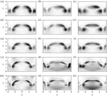
, given in figure 11 for a selection of frequencies. The amplitude functions obtained for case H1.0-T2B (shown in figure 10
a,d,g,j,m) indicate that, in this case, the disturbance growth is driven by a sinuous instability of the wake of the roughness element for all the frequencies of the forcing. This sinuous wake mode is referred to here as mode SL (sinuous lateral) and is a consequence of the out of phase instability of the lateral (
 $\partial u/\partial z$
) high-shear layers induced by the counter-rotating vortex pair. The sinuous nature of mode SL is confirmed in figure 12(a) through contours of the real part of its
 $u$
-velocity eigenfunction. Mode SL is dominant at
 $F=0.02$
in all cases, which explains the agreement between the growth rates observed in figure 10(b) for cases H1.0-T1, H1.0-T2A and H1.0-T2B; it reaches a maximum growth rate of
 $-{\it\alpha}_{i}\approx 0.0146$
at
 $F=0.04$
and has a phase speed of
 $c_{ph}\approx 0.83$
.
Contour lines (11 and equally spaced between 0 and 1) of basic
 $u$
-velocity superimposed over shaded contours of the amplitude functions obtained after taking the Fourier transform over time on
 $y{-}z$
planes at
 $x=140$
(dark for high and light for low amplitude): (a,d,g,j,m) for case H1.0-T2B; (b,e,h,k,n) for case H1.0-T2A and (c,f,i,l,o) for case H1.0-T1; (a–c)
 $F=0.04$
; (d–f)
 $F=0.06$
; (g–i)
 $F=0.08$
; (j–l)
 $F=0.12$
; and (m–o)
 $F=0.14$
.

Contours of the real part of the Fourier transformed
 $u$
-velocity on
 $y{-}z$
planes at
 $x=140$
: (a) mode SL obtained case H1.0-T2B at
 $F=0.04$
; (b) mode VL obtained for case H1.0-T1 at
 $F=0.06$
; and (c) mode VC obtained for case H1.0-T1 at
 $F=0.14$
.

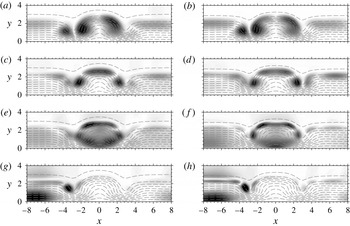
The amplitude functions obtained in the H1.0-T1 case are given in figure 11(c,f,i,l,o). In this case, the wake instability appears to be driven by a different set of modes depending on the frequency. For
 $0.04\leqslant F\leqslant 0.10$
the dominant wake mode is similar to mode SL in that both are a consequence of the instability of the lateral high-shear layers. However, in this case the oscillations of the left and right shear layers are in phase (as can be seen in figure 12
b) and the resultant wake mode, referred here to as mode VL (varicose lateral), has a varicose character. Mode VL reaches a peak growth rate of
 $-{\it\alpha}_{i}\approx 0.026$
at
 $F=0.06$
, which is approximately 1.7 times higher than that of mode SL, and has a phase speed of
 $c_{ph}\approx 0.86$
. Figure 11(l,o) show that the instability of the roughness wake for
 $F=0.12$
and
 $F=0.14$
, respectively, is driven by a mode characterised by a different near-wall maximum value of the
 $u$
-velocity (and
 $v$
-velocity) amplitude function at the roughness mid-plane. This new mode is denoted here as mode VC (varicose centred) and is associated with a varicose deformation of the low-velocity streak; the real part of its
 $u$
-velocity eigenfunction is given in figure 12(b), showing the varicose character of the wake mode. The results indicate that mode VC has a phase speed of
 $c_{ph}\approx 0.90$
, appearing for
 $F=0.12$
and reaching a maximum growth rate of
 $-{\it\alpha}_{i}\approx 0.026$
at
 $F=0.14$
. As will be shown in the next section, the new mode appears to be closely related to the Mack modes developing in the surrounding undisturbed boundary layer. However, while mode VC becomes unstable, starting from
 $x\approx 60$
as shown in figure 10(d), the
 $F=0.14$
Mack mode is stable up to
 $x\approx 120$
. The eigenfunctions obtained here for modes SL, VL and VC are in excellent agreement with the biglobal stability results obtained by Paredes et al. (Reference Paredes, De Tullio, Sandham and Theofilis2013) using the same basic flow considered in this work.
The wake response obtained for case H1.0-T2A is shown in figure 11(b,e,h,k,n). The highly asymmetric shape of the amplitude functions indicates that, in this case, varicose and sinuous modes have comparable amplitudes, which may explain the somewhat erratic behaviour observed for the growth of disturbances downstream of the roughness element. Note that a linear interaction between sinuous and varicose modes of comparable amplitudes will lead to a constructive interference on one side of the wake and a destructive interference on the other (see figure 12(a,b) for reference). This leads to the amplitude functions extracted from the numerical data using the Fourier transform being asymmetric. In particular, we note that in the
 $F=0.04$
and
 $F=0.014$
amplitude functions, shown respectively in figure 11(b,n), the dominant contributions appear to come from mode VL and mode VC, respectively. In fact, the disturbance growth rates associated with the above frequencies for case H1.0-T2A agree well with those observed for case H1.0-T1 (see for example figure 10
d for
 $x>120$
), where the varicose modes are clearly dominant. On the other hand, the
 $F=0.06$
and
 $F=0.08$
amplitude functions, shown respectively in figure 11(c,h), are closer to mode SL than to mode VL and the growth of disturbances downstream of the roughness element roughly agrees with that observed for case H1.0-T2B (see figure 10
b,c).
The excitation of wake modes appears to follow two main paths. One mechanism is based on the interaction between the boundary-layer disturbances and the basic flow distortion induced by the roughness element, whereby disturbances amplify particularly in the upstream and/or downstream reverse flow regions. These disturbances then feed the instability of the wake. This mechanism is responsible for the excitation of the sinuous mode for case H1.0-T2B. It can be seen from figure 10 that the boundary-layer disturbances experience a strong amplification in the downstream separation bubble for case H1.0-T2B and that this amplification correlates with the amplitude of the most unstable wake modes in figure 10(b,c). This mechanism appears to favour the excitation of sinuous modes, at least for the case of a generic three-dimensional disturbance environment. The above observations would be explained by the presence of a least-damped global mode of the roughness wake that is sinuous in nature (as in bluff body wakes) and is excited by the forcing. However, the validity of this observation should be tested with further investigations based, for example, on global stability analysis.
Visualisation of the disturbance field inside the boundary layer at
 $y=0.87$
, showing the excitation of the wake modes. Contours of the real part of the Fourier transformed
 $v$
-velocity (a) and
 $u$
-velocity (b,c). The contours are normalised by the maximum value attained in the plane shown: (a) case H1.0-T2B for
 $F=0.06$
; (b) case H1.0-T1 for
 $F=0.06$
; and (c) case H1.0-T1 for
 $F=0.14$
.

The other mechanism is due to the interaction between the boundary-layer modes and the wake of the roughness element and appears to be responsible for the excitation of the varicose modes. In this case, the wake mode excitation is possible because the phase speeds of the boundary-layer modes (
 $c_{ph}\approx 0.88$
for the first mode and
 $c_{ph}\approx 0.92$
for the Mack mode) are comparable to those of modes VL and VC. A synchronisation between the boundary-layer modes and the roughness wake modes (which would be possible through an interaction between the boundary-layer modes and the non-parallel roughness wake) would lead to the continuous excitation of the wake modes as the boundary-layer modes grow downstream of the roughness elements.
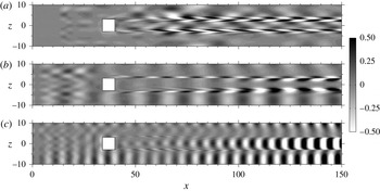
Flow visualisations corroborate the above proposals. A snapshot of the evolution of
 $u$
-velocity disturbances inside the boundary layer for case H1.0-T2B, showing the excitation and subsequent growth of mode SL for
 $F=0.06$
, is given in figure 13(a). It can be seen that sinuous perturbations appearing immediately downstream of the roughness element seem to evolve naturally into mode SL without the interference of the disturbances developing in the surrounding boundary layer, indicating that the first of the mode excitation mechanisms discussed above is dominant in this case. The evolution of these sinuous perturbations in the downstream separation bubble is responsible for the sudden disturbance amplification observed immediately downstream of the roughness element in figure 10 for case H1.0-T2B. Snapshots of the excitation and subsequent evolution of wake modes at
 $F=0.06$
and
 $F=0.14$
for case H1.0-T1 are shown in figure 13(b,c), respectively. It can be seen that the excitation of mode VL (figure 13
b) and mode VC (figure 13
c) are highly correlated with the development of, respectively, a two-dimensional first mode and a two-dimensional Mack mode in the surrounding boundary layer. Note that for
 $F=0.06$
the wake disturbances are initially sinuous and become varicose further downstream, where mode VL becomes dominant, explaining the growth rate increase observed in figure 16(b) starting from about
 $x=100$
. Figure 13(c) shows that at
 $F=0.14$
the Mack mode excites mode VC immediately downstream of the roughness element, where the two modes are roughly in phase. A similar scenario appears for case H1.0-T2A (not shown), where the interaction between an unstable oblique Mack mode with the roughness wake also leads to the excitation of mode VC.
4.4. Wall temperature effects on the instability of the roughness wake
The effects of wall temperature on the stability of high-speed boundary layers developing over smooth surfaces have been studied extensively (see for example Mack Reference Mack1984). It is well known that wall cooling leads to the stabilisation of the first mode of instability and a destabilisation of the Mack mode. The Mack mode destabilisation is thought to be due to the local Mach number increase associated with a decrease in wall temperature. Cooling also affects the frequency of the most unstable Mack mode, since this is highly ‘tuned’ with the boundary-layer thickness (i.e. its most unstable wavelength is roughly twice the boundary-layer thickness).
This section provides a discussion of the effects of wall cooling on the stability of the wake induced by the roughness element for case H1.0. The study is carried out using type T1 inflow perturbations, as in this case the wake response is such that an analysis of the effects of wall temperature on the development of modes SL, VL and VC is possible. The analysis is performed through comparisons between the results obtained for cases H1.0-T1 and C1.0-T1. Note that, in order to minimise local Reynolds number effects, the roughness Reynolds number for case C1.0-T1 is chosen to be the same as for case H1.0-T1, which entails decreasing the simulation Reynolds number from
 $\mathit{Re}_{{\it\delta}_{0}^{\ast }}=8200$
to
 $\mathit{Re}_{{\it\delta}_{0}^{\ast }}=4135$
. It is important to note that, while cooling typically leads to a reduction of the boundary-layer thickness, in our case the non-dimensional boundary-layer thickness for case C1.0-T1 is larger than for case H1.0-T1. This is a combined effect of the decrease of
 $T_{w}$
and
 $\mathit{Re}_{{\it\delta}_{0}^{\ast }}$
and leads to the reduction of the non-dimensional frequency of the most unstable Mack mode, as shown below.
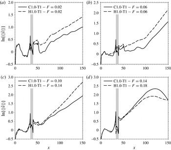
Figure 14 gives a comparison of the evolution of
 $v$
-velocity disturbances inside the boundary layer for a selection of the most representative frequencies. The flow instability observed in figure 14(a,b) is driven by the wake modes SL and VL, respectively. The amplitudes of the two modes are lower for the cooled-wall case, despite the amplitude of the boundary-layer disturbances developing upstream of the roughness element being the same for the two cases. To provide a possible explanation for this observation we note that near
 $x=52$
in figure 14(a,b) the amplitude of the boundary-layer disturbances undergoes a sudden drop, both for case H1.0-T1 and case C1.0-T1. This amplitude jump coincides with the position of the oblique shock generated downstream of the roughness element due to the flow reattachment (see figure 7
a) and is more prominent for the case C1.0-T1, where the reattachment shock is strongest. The results show that the shock tends to damp disturbances with frequencies lower than approximately
 $F=0.14$
and indicate that the reattachment shock plays a role in the excitation of the boundary-layer modes and the wake modes. Despite the variation in mode amplitudes, the growth rates of the modes SL and VL are reduced very slightly after a reduction of the wall temperature by factor of two, indicating that the effect of wall cooling on the development of these modes is very weak. This also shows that the roughness Reynolds number is an effective parameter for the characterisation of the stability of the roughness wake when this is dominated by modes SL and VL (recall that the simulation Reynolds number is lower for case C1.0-T1 than for case H1.0-T1). The amplitude functions obtained for the two cases are compared in figure 15(a,b) for mode SL and figure 15(c,d) for mode VL, showing that the influence of wall temperature is also weak for the mode eigenfunctions.
Evolution of
 $v$
-velocity disturbances inside the boundary layer for cases H1.0-T1 and C1.0-T1. The shaded grey area indicates the position of the roughness element: (a)
 $F=0.02$
, showing the evolution of mode SL; (b)
 $F=0.06$
, showing the evolution of mode VL; (c)
 $F=0.10$
for case C1.0-T1 and
 $F=0.14$
for case H1.0-T1, showing the evolution of modes VC; (d)
 $F=0.14$
for case C1.0-T1 and
 $F=0.18$
for case H1.0-T1, showing the Mack mode evolution.

Contour lines (11 and equally spaced between 0 and 1) of basic
 $u$
-velocity superimposed over shaded contours of the amplitude functions obtained after taking the Fourier transform over time on
 $y{-}z$
planes at
 $x=140$
(dark for high and light for low amplitude): (a,c,e,g) case C1.0-T1 and (b,d,f,h) case H1.0-T1; (a,b)
 $F=0.02$
; (c,d)
 $F=0.06$
; (e)
 $F=0.10$
; ( f)
 $F=0.14$
; (g)
 $F=0.14$
; and (h)
 $F=0.18$
.

The influence of wall cooling is much more pronounced for the mode VC instability. While the dominant mode VC for case H1.0-T1 has a frequency of
 $F=0.14$
, the maximum mode VC growth rate for case C1.0-T1 is obtained for
 $F=0.10$
. The evolution of the dominant mode VC obtained for the two cases is given in figure 14(c), showing that cooling also leads to a reduction of the growth rate, which for case C1.0-T1 is
 $-{\it\alpha}_{i}\approx 0.0175$
; approximately 33 % lower than that obtained for case H1.0-T1. The corresponding amplitude functions are given in figure 15(e,f), respectively. It can be seen that cooling also leads to a modification of the mode VC eigenfunction, particularly in the near-wall region, where two local maxima appear in the
 $u$
-velocity eigenfunction obtained for case C1.0-T1 in contrast with the single local maximum found for case H1.0-T1. Overall, the results indicate that mode VC is of a different nature compared to modes SL and VL, while it shows similarities with the Mack mode instability. A reduction of the non-dimensional frequency of the most unstable mode VC correlates well with the increased non-dimensional boundary-layer thickness of case C1.0-T1. Therefore, mode VC is tuned with the boundary-layer thickness, similarly to what is observed for the Mack mode instability. However, while the Mack modes become more unstable with wall cooling, mode VC tends to be damped despite the Mach number in the roughness wake being higher for case C1.0-T1 than for case H1.0-T1. The results presented here suggest that mode VC plays an important role in the roughness-induced transition at high speeds.
The effects of wall cooling on the Mack mode instability are highlighted in figure 14(d), which shows the amplification experienced by the most dangerous Mack modes for case C1.0-T1 (
 $F=0.14$
) and case H1.0-T1 (
 $F=0.18$
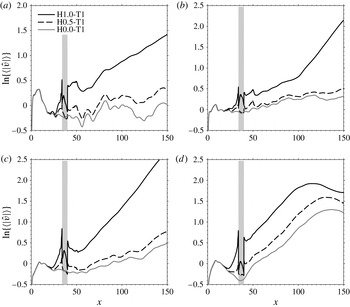
). It can be seen that the increase in non-dimensional boundary-layer thickness and local Mach number associated with the wall temperature decrease leads to frequency reduction and a growth rate increase for the most unstable Mack modes. The amplitude functions given in figure 15(e,f) show that the disturbance growth observed in figure 14(d) is indeed due to the Mack mode development in the undisturbed boundary layer surrounding the wake of the roughness element. Note that the spanwise asymmetry of the inflow forcing about the roughness mid-plane results in asymmetric Mack mode amplitude functions.
Evolution of
 $v$
-velocity disturbances inside the boundary layer for cases H1.0-T1, H0.5-T1 and H0.0-T1. The shaded grey area indicates the position of the roughness element: (a)
 $F=0.02$
; (b)
 $F=0.06$
; (c)
 $F=0.14$
; (d)
 $F=0.18$
.

4.5. Discussion of the effects of roughness elements on the flow instability
This section is devoted to a quantification of effects of roughness on the boundary-layer instability, which is carried out in order to determine whether the roughness element analysed in the previous sections may lead to an acceleration of the laminar–turbulent transition process. To this end, we perform a direct comparison between the results obtained for case H1.0-T1 and those obtained for a roughness element with half the height (case H0.5-T1) and for a smooth flat plate (case H0.0-T1). Note that in the above three cases the simulation Reynolds number
 $\mathit{Re}_{{\it\delta}_{0}^{\ast }}=8200$
is kept constant, hence the roughness Reynolds numbers are
 $\mathit{Re}_{h}=331$
,
 $\mathit{Re}_{h}=60$
and
 $\mathit{Re}_{h}=0$
, respectively, as reported in table 1.
Figure 16 shows the evolution of
 $v$
-velocity disturbances inside the boundary layer for cases H1.0-T1, H0.5-T1 and H0.0-T1 for a selection of frequencies. It can be seen that, as expected, sufficiently upstream of the roughness element the results obtained in the three cases are virtually indistinguishable and only depart from each other when the disturbances start approaching the roughness elements. In the H1.0-T1 and H0.5-T1 cases the disturbances are substantially amplified, relative to case H0.0-T1, in the upstream separation bubbles, more so for the taller roughness element of case H1.0-T1. The results obtained for case H0.5-T1 show that, after this initial amplification, the evolution of boundary-layer disturbances follows closely that observed for case H0.0-T1. Therefore, in this case, the roughness element mainly acts as a disturbance amplifier; scattering disturbance energy generated in the upstream separation bubble into the instability modes of the surrounding undisturbed boundary layer. In this case the wake of the roughness element appears to have very little effect on the stability of the boundary layer.
The boundary-layer instability follows a different path for case H1.0-T1. As already discussed in § 4.3, in this case the roughness element induces a wake that is able to sustain the growth of additional instability modes. The sinuous mode, an example of which is given in figure 16(a), has a peak growth rate approximately 30 % higher than that of the most unstable first mode (i.e. the
 $F=0.07$
and
 $k_{z}=1.1$
first mode with
 $-{\it\alpha}_{i}=0.0112$
obtained by LST and discussed in § 4.1) and approximately 35 % lower than that of the
 $F=0.18$
Mack mode (which, with a maximum LST growth rate of
 $-{\it\alpha}_{c}i=0.0223$
is the most dangerous boundary-layer mode for the flow conditions considered), the evolution of which is shown in figure 16(d). On the other hand, the growth rates of the most unstable varicose modes, shown in figures figure 16(b) (mode VL) and 16(c) (mode VC), are both approximately 17 % higher than that the
 $F=0.18$
Mack mode. In addition to the increased growth rate, the wake modes have a longer region of instability than the Mack modes. In fact, as discussed in § 4.2, the wake flow induced by the tall roughness element tends to persist for a long streamwise distance and, in addition, the growth rates of the wake modes obtained for case H1.0-T1 are not found to decrease within the computational domain. This leads us to the conclusion that the roughness element considered in case H1.0 may induce a substantial acceleration of the laminar–turbulent transition process, depending on the nature of the disturbance environment inside the boundary layer. Note also that for forcing frequencies to which the roughness wake is not receptive (i.e.
 $F=0.18$
in figure 16
d), the roughness element acts as a disturbance amplifier as for case H0.5-T1, leading to an increase of the
 $F=0.18$
Mack mode amplitude by about a factor of 2.8.
5. Conclusions
The influence of boundary-layer disturbances on the instability of the wake induced by a squared, sharp-edged roughness element in an
 $M=6$
boundary layer has been investigated using numerical simulations of the compressible Navier–Stokes equations. The investigation has uncovered two principal mechanisms responsible for the excitation of the wake instabilities and has highlighted the importance of the boundary-layer disturbance environment for the selection of the dominant excitation mechanism. The study has also shown the existence of a new wake mode with characteristics similar to those typical of the Mack mode instability and, as such, believed to be of critical importance for the roughness-induced transition in high-speed boundary layers.
The results show that a discrete roughness element with a height
 $h^{\ast }=0.54{\it\delta}_{99}$
 $(\mathit{Re}_{h}=331)$
induces a pair of strong counter rotating vortices which, through the lift-up mechanism, lead to the generation of a low-velocity streak surrounded by regions of detached high shear, which form the wake flow behind the roughness element. The roughness wake is able to sustain the growth of a number of different instabilities; a sinuous mode and a varicose mode (modes SL and VL) developing due to the instability of the lateral (
 $\partial u/\partial z$
) shear layers surrounding the streak and a new varicose mode (mode VC) which appears to be strongly connected to the Mack modes developing in laminar high-speed boundary layers over smooth surfaces. The wake mode eigenfunctions obtained from the current Navier–Stokes study are in excellent agreement with biglobal eigenfunctions obtained by Paredes et al. (Reference Paredes, De Tullio, Sandham and Theofilis2013) for the same basic flow. While the sinuous mode only reaches a peak growth rate of
 $-{\it\alpha}_{i}\approx 0.0146$
, approximately 35 % lower than that of the most dangerous Mack mode, the maximum growth rates registered for modes VL and VC are approximately 12 % higher than the dominant Mack mode growth rate and, in addition, they remain unstable for a long distance downstream of the roughness element. Therefore, the roughness element may lead to a substantial acceleration of the laminar–turbulent transition process. Whether this is the case in practice depends on the nature of the boundary-layer disturbance environment. The present study shows that there are two main mechanisms responsible for the excitation of the wake modes. Upon reaching the roughness element, the boundary layer disturbances are likely to excite damped global modes in the recirculation bubble, which in turn feed the instability of the roughness wake. This mechanism favours the excitation of mode SL and is found to be dominant in the case of a generic three-dimensional perturbation field given by the disturbances induced inside the boundary layer by the acoustic waves propagating in the free stream obliquely to the flow direction. The other important wake mode excitation mechanism is based on the fact that the phase speeds of the first mode (
 $c_{ph}\approx 0.88$
) and the Mack mode (
 $c_{ph}\approx 0.92$
), developing in the undisturbed boundary layer surrounding the wake, are sufficiently close to those of modes VL (
 $c_{ph}\approx 0.86$
) and VC (
 $c_{ph}\approx 0.90$
), respectively. Therefore, a nonlinear interaction between the boundary-layer modes and the non-parallel roughness wake may easily provide the matching of the wavenumbers required for the excitation of the wake modes. This mechanism appears to be responsible for the excitation of the most unstable wake modes (i.e. the varicose modes), suggesting that the roughness element considered in this work may substantially accelerate the laminar–turbulent transition, provided the boundary-layer modes come into interaction with its wake.
A study of the effects of wall temperature on the wake instability reveals that wall cooling has limited effects on the shear-layer modes (modes SL and VL) while it affects greatly the development of mode VC. Similarly to what is typically observed for the Mack mode instability, mode VC is found to be highly tuned to the local boundary-layer thickness. In contrast to the Mack mode instability, however, mode VC is found to be damped by cooling. In fact, cooling is found to be stabilising for all the roughness-wake modes.
Acknowledgements
The authors would like to acknowledge the financial support of the EU through the FP-7 LAPCAT II Project and the computational time on the Hector supercomputer provided by the UK Turbulence Consortium (EPSRC grant EP/G069581/1). Constructive comments by the anonymous referees are also gratefully acknowledge.