


Introduction
A product assembly should be disassembled for reuse, recycling, remanufacturing, and refurbishing to minimize its environmental impact during the End-of-Life (EoL) cycle. In this regard, disassembly is a prerequisite for disassembling the parts and ensuring that the retrieved parts preserve their original form and functionality as per assembly information (Yokota and Brough, Reference Yokota and Brough1992; Ong et al., Reference Ong, Chang and Nee2021; Anil Kumar et al., Reference Anil Kumar, Bahubalendruni, Madhu Balan and Eswaran2023; Zhu et al., Reference Zhu, Xu, Wang, Yang and Fan2023). DSP aims to obtain a disassembly sequence that satisfies constraints and metrics (Gungor and Gupta, Reference Gungor and Gupta1998; Lambert and Gupta, Reference Lambert and Gupta2004). DSP problems are categorized based on disassembling the parts sequentially or in parallel. In complete sequential DSP, all the product parts are disassembled one at a time in all the disassembly levels or steps, whereas in the case of selective sequential DSP, product parts are disassembled until the target (selective) part. Correspondingly, in complete parallel DSP, depending on the nature of the product assembly, more than one part is disassembled in at least one of the disassembly levels until all the parts are disassembled. In contrast, in complete selective parallel DSP, more than one part is disassembled in at least one of the disassembly levels up to the target part considered (Ong et al., Reference Ong, Chang and Nee2021, Chand and Ravi, Reference Chand and Ravi2023).
Due to the linear nature of the sequential DSP as well as the conditions considered during disassembly, it incurs more disassembly levels or steps to complete the disassembly process, especially for large, complex products. Parallel DSP is studied in this article to deal with this problem. The first and foremost constraint to be satisfied to get the disassembly sequence involving parallel parts is the precedence condition. The parts are disassembled at each disassembly level only if their predecessors have already been disassembled in one of the previous levels. This is the constraint several researchers have considered in their study (Zhou et al. Reference Zhou, Liu, Pham, Wenjun Xu, Ji and Liu2019; Guo et al., Reference Guo, Zhou, Abusorrah, Alsokhiry and Sedraoui2021). Since the precedence constraint conveys only the order of disassembly of the individual parts of the product, the stability constraint of the product must also be considered in the disassembly process to obtain the disassembled parts in a safe and stable manner. The stability constraint provides three types of information about which part possesses permanent stability, partial stability, or no stability concerning other product parts. This data helps plan the disassembly process to obtain all the parts without damage. This requires a new representation to consolidate these three types of information from stability data before starting the disassembly process. By analyzing the properties of the precedence and stability data of the product assembly with the graph representation, the stability data with the precedence graph of the product assembly need to be combined without referring to the stability data again. This simplifies and reduces the size of our problem to obtain the disassembly sequence. Few researchers have considered stability constraints for sequential DSP in their studies (Anil Kumar et al., Reference Anil Kumar, Bahubalendruni, Prasad and Sankaranarayanasamy2021; Gunji et al., Reference Gunji, Pabba, Rajaram, Sorakayala, Dubey, Deepak, Biswal and Bahubalendruni2021). Since DSP is proven to be an NP-hard combinatorial problem (Chand and Ravi, Reference Chand and Ravi2023), finding an optimal solution to DSP remains challenging when all the constraints are considered. To address this issue, authors have explored various model-free RL algorithms in their study (Atiya et al., Reference Atiya, Parlos and Ingber2003; Wang and Wang, Reference Wang and Wang2014; Zhao et al., Reference Zhao, Li, Tang and Cui2021; Allagui et al., Reference Allagui, Belhadj, Plateaux, Hammadi, Penas and Aifaoui2023). This research shows how model-free RL algorithms are utilized and addresses their limitations to obtain near-optimal solutions by considering direction changes.
A few authors showed how to employ only graph models to determine the parallel DSP in the early days – for example, Chen et al. (Reference Chen, Oliver, Chou and Chen1997), who proposed a more straightforward mating graph and produced data structures to enable an effective parallel DSP. From a purely geometric perspective, sequence prediction becomes more challenging as the product’s component count rises (Dutta and Woo, Reference Dutta and Woo1995). Taking sequence-dependent operation times into account while determining the disassembly level and disassembly sequence is challenging, especially in the parallel DSP. Kang et al. (Reference Kang, Lee, Xirouchakis and Persson2001) suggested an extended process graph for sequence-dependent operation times and integer programming formulations to simultaneously determine the disassembly sequence and disassembly levels. The proposed approach works best for small and medium-sized products. Gulivindala et al. (Reference Gulivindala, Bahubalendruni, Chandrasekar, Ahmed, Abidi and Al-Ahmari2021) proposed disassembly sequence prediction using an enhanced genetic algorithm for Industry 4.0 applications. Bahubalendruni and Varupala, Reference Anil Kumar, Bahubalendruni, Prasad and Sankaranarayanasamy2021 proposed an automated disassembly sequence generation method for waste electronic and electric products.
Disassembling large-scale industrial products in parallel has attracted several researchers. Zhang and Zhang, Reference Zhang and Zhang2010 proposed cooperative disassembly sequence planning to disassemble large and complex products by constructing a hybrid graph to understand the properties among product components. The authors applied branch-and-bound to obtain a hierarchical disassembly tree from the hybrid graph. Ren et al. (Reference Ren, Tian, Zhao, Yu and Zhang2017) proposed an artificial bee colony algorithm-based cooperative disassembly planning to optimize disassembly time and profit. The authors considered precedence, exclusion, and a cooperative matrix to understand the properties between the components. The authors suggested a genetic algorithm (GA)-based job allocation plan with cooperative DSP.
Zhu et al. (Reference Zhu, Xu, Su and Dong2020) proposed a multi-manipulator-based parallel DSP using an enhanced frog leaping algorithm (Eusuff et al., Reference Eusuff, Lansey and Pasha2006). In order to make the objective function realistic for large-scale products, they have considered disassembly preparation time along with disassembly time. An encoding strategy was initially used to represent the disassembly sequence and manipulators assigned to each part. Parallel allocation of the parts to manipulators based on the disassembly time was suggested in the decoding strategy. Both strategies improve the optimization capability of the proposed algorithm. On large-scale products, the suggested algorithm’s efficacy was confirmed. Tseng et al. (Reference Tseng, Chang and Chung2022) applied an improved Particle Swarm Optimization (PSO) algorithm (Kennedy and Eberhart, Reference Kennedy and Eberhart1995) to solve the parallel DSP problem. The authors proposed an optimization method for arranging multiple manipulators to disassemble parts in parallel. The overall objective of the problem was to minimize the time required to complete the disassembly process. The proposed approach was compared with three recent works and the products of different complexities. The proposed algorithm converged to an optimal solution faster than GA and ACO.
Ren et al. (Reference Ren, Chaoyong, Fu, Huajun and Guangdong2018) proposed an encoding scheme that creates a vector list for the disassembly sequence and another list for the assignment of manipulators. The decoding scheme evaluates the disassembly sequence with regard to disassembly time. However, the effectiveness of the proposed approach needs to be addressed using other factors like cost, time, and profit with selective or partial disassembly. The authors introduced a new version of the Ant Colony Optimization (ACO) algorithm (Xing et al. (Reference Xing, Wu and Qu2021)) to address the challenges of solving asynchronous parallel DSP. The authors considered execution time, preparation time, and the collision matrix in the study and analyzed the performance of the proposed approach with a case study and generated an optimal solution in a reasonable time. Along with focusing on obtaining a disassembly sequence, minimizing the complexity and improving the efficiency of the proposed approach have been studied by researchers. One such work was presented by Tao et al. (Reference Tao, Bi, Zuo and Nee2018), where the authors propose an automated self-decomposed precedence matrix for disassembly. The Tabu search algorithm was adopted to improve exploration ability, energy benefit, and disassembly time. However, they did not compare their approach with other heuristic algorithms for exploration strategy.
Kim and Lee, Reference Kim and Lee2017 considered the selective DSP with sequence-dependent setup costs to find multiple target components by a disassembly operation. They proposed a branch-and-bound algorithm to minimize the solution space and derive a bounding condition for lower and upper constraints. Smith and Hung, Reference Smith and Hung2015 presented the difficulties in removing parts due to interlocking, extra reorientations, and extra movements during the sequential disassembly process. They have applied theory on a modular design to a product to cluster parts into a block and adapted recursive rules to separate the blocks to disassemble more than one component. Zhang et al. (Reference Zhang, Wu, Li, Ren and Zhu2022) proposed a selective parallel DSP using a novel hybrid genetic algorithm to optimize disassembly time and cost. The authors have shown the efficacy of the suggested approach on transmission boxes.
Many authors solved the DSP using graphs and adopted heuristics and metaheuristic algorithms because the problem is combinatorial. Zhang et al. (Reference Zhang, Yu, Hu, Pei and Ma2014) used fuzzy-rough sets in their study. The mapping model was constructed to understand the characteristics of the product parts. The authors have adopted the mapping model’s knowledge universe and disassembly membership functions. The proposed approach validated two products of different scales. However, it may not guarantee the optimal result for large-scale, complex products. In product refurbishment, disassembly is the prerequisite to test individual parts’ functionality and replace those parts if found defective. To make this process efficient, and that too in a parallel disassembly environment, Pistolesi and Lazzerini, Reference Pistolesi and Lazzerini2019 proposed a two-stage methodology to obtain parallel DSP using the Tensorial Memetic Algorithm (TeMA) for optimizing time while disassembling and counting rotations. Authors got Pareto-optimal seeds in the first stage based on time and degree of parallelism. In the next stage, the authors used TeMA to carry out the local search around the Pareto-optimal regions to improve the secondary objective further. The proposed algorithm was tested on two products following refurbishment processes and compared with other many-objective algorithms. Also, an improved RL approach has been used for solving sequential DSP problem (Chand and Ravi, Reference Chand and Ravi2024b).
In summary, despite a few techniques mentioned above in the parallel DSP, the challenge exists in obtaining a near-optimal disassembly sequence involving parallel parts to complete the disassembly process at lower levels by minimizing direction changes. It is a challenge for the decision-maker to select the part(s) that satisfy the precedence, stability, and objective of the problem throughout the disassembly process using RL. However, to the best of our knowledge, we did not find research papers in the literature addressing stability data and modeling as a model-free tabular based RL problem for parallel DSP. This motivated us to propose a novel two-stage model-free RL technique to tackle this challenge. The proposed methodology is suitable for complete product disassembly, where the retrieved parts can be utilized for remanufacturing purposes in the later stages.
The following are the main contributions of this study.
-
• This work presents the process involved in innovatively integrating the stability data with the precedence graph, called the stability-integrated precedence graph, as well as the steps involved in generating different part combinations of the product assembly up to a degree of parallelism of three by satisfying the constraints in the initial stage.
-
• The second stage shows a model-free reinforcement learning formulation of the parallel DSP problem. ASALD-Q algorithm is proposed to obtain the optimal parallel DSP that involves more parallel parts, thereby reducing the disassembly levels by minimizing direction changes.
-
• A novel adaptive mechanism is proposed to dynamically adjust the ASALD parameters according to the previous performance to circumvent becoming trapped in local optima during search space exploration.
-
• To deal with the combinatorial nature of the problem, a sparse Q-table representation is proposed instead of a dense representation to make the proposed algorithm appropriate for practical industrial products.
-
• The proposed approach is utilized on three different-sized products to showcase its effectiveness. Additionally, the results are compared with another model-free RL algorithm for two exploration strategies. The proposed approach has been validated using a complex product from previous literature.
The remainder of the article is organized as follows: the problem description and the mathematical model are described in Section “Problem description”; background concepts and the proposed methodology are described in Section “Proposed methodology”; results and discussion of the research work are discussed in Section “Results and discussions”; and finally, the concluding remarks are given in Section “Conclusion.”
Problem description
To address the problem of parallel DSP, initially, the disassembly model that uses precedence and stability constraints is illustrated followed by mathematical model for parallel DSP.
Precedence constraint
Consider an eight-part product assembly reported in Anil Kumar et al. (Reference Anil Kumar, Bahubalendruni, Prasad and Sankaranarayanasamy2021); Chand and Ravi, Reference Chand and Ravi2024b and the same is shown in Figure 1. Figure 1(a) shows the 3D view of the product assembly and Figure 1(b) shows the exploded view of the assembly. We consider the same product to illustrate our methodology in the upcoming section. An assembled product is a non-empty set of stable parts with no more than one connection to other components. Each part of the product is denoted by i, where i = 1 to N, representing the number of parts. Any part i considered for disassembly connects with other parts of the product, creating a dependency among the parts. Knowing this information about each part’s dependence on other parts (also called precedence) in the initial stage of the disassembly helps to complete the disassembly process in an ordered manner. This information can be represented as a graph structure called a disassembly precedence graph. Graph G is defined by vertices V and edges E, where V represents the product’s components and E represents their connections. Figure 2 shows the precedence graph for the eight-part product assembly.
Three-dimensional model of an eight-part product assembly: (a) Assembled view and (b) Exploded view.

Disassembly precedence graph.

From the figure, we can describe the components V and E of G, where
$ V=\left\{1,2,3,4,5,6,7,8\right\} $
 , and
$ E=\left\{\left(4,3\right),\left(3,1\right),\left(5,1\right),\left(6,1\right),\left(7,2\right),\left(8,2\right),\left(2,1\right)\right\} $
 . Each pair of vertices (x, y) in E represents an ordered pair of vertices, where x indicates the predecessor of y and y is the immediate successor of x. This means that part x must be disassembled before disassembling part y. While disassembling, each product part satisfies this constraint must be ensured. The precedence graph can also be represented as an adjacency matrix (Zhu et al., Reference Zhu, Xu, Wang, Yang and Fan2023). An adjacency matrix for a graph G (V, E) consists of a two-dimensional array of size n × n defined in Eq. (1).

Based on the number of vertices and edges in the precedence graph, the adjacency matrix representation of a product is obtained, and the same is shown for the eight-part product assembly in Figure 3(a). The matrix cells indicate the presence (denoted by 1) and absence of corresponding edges (denoted by 0) in the precedence graph. For example, matrix cell (2,1) is denoted as 1 due to the presence of an edge from vertex 2 to vertex 1, as shown in Figure 2. Similarly, matrix cell (4,2) is denoted as 0 due to the absence of an edge from vertex 4 to vertex 2 in the graph.
Matrix representation of an eight-part product: (a) Precedence matrix and (b) Stability matrix.

Given the precedence graph of the product, parallel DSP involves identifying more than one part of the product that can be disassembled in parallel in at least one of the disassembly levels, satisfying the precedence and other conditions (Lambert and Gupta, Reference Lambert and Gupta2004). The disassembly level serves as a measure of disassembly progression and is expressed as the number of parts disassembled satisfying the constraints (Lambert and Gupta, Reference Lambert and Gupta2004). Each level could represent a specific stage in the disassembly process, where deeper levels mean that more parts have been removed. Since the number of parallel parts may increase depending on the precedence conditions of the product, we assume that the degree of parallelism is 3, which means that the maximum number of parallel parts that can be disassembled in any of the disassembly levels is 3. If, at any disassembly level, parallel parts cannot be considered for disassembly due to a violation of conditions, then individual parts are considered.
For example, the following parallel parts are considered during disassembly based only on the precedence conditions, as shown in Figure 2 are {(4,5), (4,6), (4,7), (4,8), (5,6), (5,7), (5,8), (6,7), (6,8), (7,8)}. Individual parts 1, 2, and 3 are not considered in parallel combinations due to their dependence on the predecessors. From these available part combinations, as well as based on the disassembly direction of each part, the decision-maker has to intelligently identify or plan whether individual parts or parallel parts are considered during the disassembly process, satisfying the conditions, thereby returning a parallel disassembly sequence consisting of the order of all the parts of the product that are disassembled successfully. To refine infeasible parallel parts combinations and to obtain all the parts of the product without any damage, we use the product’s stability-integrated precedence condition and disassembly direction.
Stability constraint
The precedence graph helps to obtain the disassembly sequence in the order of the dependency of the parts based on their accessibility. However, this alone is insufficient to obtain the disassembly sequence in a stable manner. To address this issue, the stability constraint of the product has been used while disassembling. A stability constraint is an n × n matrix, where n is the number of product parts. The stability matrix for the eight-part product assembly is shown in Figure 3(b).
Let
$ S=\left[{S}_{ij}\right] $
 represent the stability between the parts i and j for a product, which is defined as

The stability matrix shows three types of information based on the relationship maintained by the parts for any one of the three-dimensional axes. They are called permanent, partial, and no stability.
-
• Permanent stability: Permanent stability is where two product components retain their relationship regardless of orientation (Anil Kumar et al., Reference Anil Kumar, Bahubalendruni, Prasad and Sankaranarayanasamy2021; Gunji et al., Reference Gunji, Pabba, Rajaram, Sorakayala, Dubey, Deepak, Biswal and Bahubalendruni2021). It ensures that the product assembly remains secure after any part is disassembled and does not collapse, shift, or become unsafe. This stability is essential to maintain the integrity of the remaining parts throughout and after the disassembly process. For example, Figure 1 shows that since parts 5 and 6 are permanently stable due to the inherent self-arrangement with the base part, disassembling them leaves the rest of the product assembly safe. Also, disassembling any other parts from the product does not impact parts 5 and 6. Hence, these parts are called permanent stability, and such parts are filled with two in the stability matrix shown in Figure 3(b). Similarly, parts 7 and 8 also possess permanent stability with the base part due to the inherent property of physical connectors used in the assembly. Here, too, disassembling parts 7 and 8 does not impact other parts like part 2 because they will remain partially stable with the base part.
-
• Partial stability: Partial stability refers to a relationship that is maintained along only one axis (Anil Kumar et al., Reference Anil Kumar, Bahubalendruni, Prasad and Sankaranarayanasamy2021). Due to this, the stability of the product assembly during disassembly is partially maintained, ensuring that the intermediate parts remain stable. As the parts are disassembled during disassembly some of the parts may become stable in only one axis, as supposed to be stable in more than one axis due to the disassembly of their supported/dependent parts. The product assembly must remain safe and stable as parts are disassembled in parallel or sequentially. For example, Figure 1 shows that even after disassembling parts 7 and 8, part 2 does not fall immediately because the base part supports it. Similarly, after disassembling part 4, part 3 still provides partial stability in one of the axes due to the support given by part 2. Hence, matrix cells (1, 2) and (2, 3) in Figure 3(b) are filled with one.
-
• No stability: It occurs when the center of gravity of the two product components does not coincide, causing the parts to lose their current contact (Anil Kumar et al., Reference Anil Kumar, Bahubalendruni, Prasad and Sankaranarayanasamy2021). For example, from Figure 3(b), matrix cells (1,3) and (1,4) are filled with 0 because parts 3 and 4 do not have any contacts with the base part.
The stability graph based on the stability matrix will show how parts support each other, and the integration of the same with the precedence graph is illustrated in Section “Results and discussions.”
Disassembly direction
Based on the precedence and stability constraints of the product, the feasible part to disassemble from the product is identified. However, the challenge lies in identifying the feasible direction to be considered to retrieve the corresponding part safely. Since each part can be retrieved in different directions based on the geometry of the product, one of the feasible directions must be considered as part of the input requirement well before starting the disassembly process.
In this work, we have assumed that each part is disassembled in only one of the six principal directions, even though some of the parts can have multiple feasible disassembly directions due to the self-arrangement of the product. For example, the disassembly direction for all eight parts of the product is shown in Table 1. However, Anil Kumar et al. (Reference Anil Kumar, Bahubalendruni, Prasad and Sankaranarayanasamy2021) and Gulivindala et al. (Reference Gulivindala, Bahubalendruni, Chandrasekar, Ahmed, Abidi and Al-Ahmari2021) provide additional details related to the generation of the disassembly direction for the product.
Disassembly direction of an eight-part product

Table 1. Long description
The table consists of two columns. The first column is titled Part number and the second column is titled Direction.
* Part number 1 has a direction of plus Z.
* Part number 2 has a direction of plus Z.
* Part number 3 has a direction of minus X.
* Part number 4 has a direction of plus X.
* Part number 5 has a direction of minus Y.
* Part number 6 has a direction of minus Y.
* Part number 7 has a direction of plus Z.
* Part number 8 has a direction of plus Z.
Disassembly sequences
Once the precedence, stability, and direction constraints for any product are given, our next job is to obtain the feasible disassembly sequence satisfying all the constraints and minimizing direction changes. Due to the nature of the product and its constraints, the product may have several feasible and infeasible disassembly sequences. We will consider the eight-part product to show some of the feasible disassembly sequences satisfying the constraints.
The sample list of feasible disassembly sequences for the eight-part product, along with the parallel parts and direction changes for illustration purposes, is shown in Table 2. All the sequences shown in the table satisfy the precedence and stability constraints of the product. The bottom four sequences have at least two parallel parts in the sequence (called parallel disassembly sequences), but the remaining ones have zero parallel parts (called sequential disassembly sequences). Also, a parallel disassembly sequence consumes fewer direction changes than a sequential one, as shown in Table 2. During the remanufacturing stage, the optimal feasible parallel disassembly sequence with fewer direction changes will be considered.
List of feasible disassembly sequences for an eight-part product

Table 2. Long description
The table consists of four columns: Sl. no., Disassembly sequence, No. of parallel parts, and No. of direction changes.
* Row 1: Sequence 7-5-4-6-8-3-2-1 with 0 parallel parts and 6 direction changes.
* Row 2: Sequence 6-8-4-3-5-7-2-1 with 0 parallel parts and 5 direction changes.
* Row 3: Sequence 8-6-5-4-7-3-2-1 with 0 parallel parts and 5 direction changes.
* Row 4: Sequence (5,6)-8-4-3-7-2-1 with 2 parallel parts and 4 direction changes.
* Row 5: Sequence (7,8)-6-5-4-3-2-1 with 2 parallel parts and 4 direction changes.
* Row 6: Sequence (5,6)-(7,8)-4-3-2-1 with 4 parallel parts and 4 direction changes.
* Row 7: Sequence (7,8)-4-3-(5,6)-2-1 with 4 parallel parts and 4 direction changes.
On the other hand, some sequences violate at least one constraint, called infeasible disassembly sequences. The sample list of infeasible disassembly sequences for the eight-part product is shown in Table 3. The bottom two disassembly sequences violate precedence and stability constraints, whereas the initial sequence violates only the precedence constraint because part 2 must be disassembled after disassembling parts 3, 4, 7, and 8. Our proposed methodology will always obtain an optimal feasible disassembly sequence for any product, which will be discussed in Section “Results and discussions.”
List of infeasible disassembly sequences for an eight-part product

Table 3. Long description
The table consists of three columns: Sl. no., Disassembly sequence, and Reason.
* Row 1: Sl. no. 1. Disassembly sequence 2-5-7-4-6-8-3-1. Reason: Precedence constraint is violated.
* Row 2: Sl. no. 2. Disassembly sequence 1-4-5-7-8-2-3-6. Reason: Precedence and stability constraints are violated.
* Row 3: Sl. no. 3. Disassembly sequence 3-4-8-7-5-6-1-2. Reason: Precedence and stability constraints are violated.
Mathematical model
The following are the assumptions considered in our study.
-
i. All the parts of the product are in working condition.
-
ii. There are no uncertain conditions considered while disassembling.
-
iii. The product parts are disassembled, retaining their original geometry and shape.
-
iv. This work considers nondestructive parallel disassembly.
-
v. The stability matrix and precedence relationship of the product are provided in advance.
-
vi. The feasible principal direction is considered for each part of the product to determine its retrieval.
Below is a summary of the decision variables used in the mathematical model.
$ {x}_{ij}=1 $
 if part
$ {p}_i $
 is disassembled in the
$ j\mathrm{th} $
 level of the sequence, and 0 otherwise.
$ {y}_a=1 $
 if a part is selected from part combinations, and 0 otherwise.
$ {w}_{kl}=1 $
 if there is a direction change occurs between disassembly levels k and l, and 0 otherwise.
The mathematical model of the parallel DSP to minimize direction changes with different constraints is stated below:


subject to


The objective {Eq. [3]} is to minimize the number of disassembly levels the agent takes to obtain the complete disassembly sequence. The objective {Eq. [4]} is to maximize the number of parallel parts in the disassembly sequence to promote parallel disassembly. The objective {Eq. [5]} is to minimize the direction changes between the disassembly levels. Constraint {Eq. [6]} ensures that each part of the product is disassembled only once. Constraint {Eq. [7]} indicates that precedence must be satisfied before disassembling a part. Constraint {Eq. [8]} ensures that each component must be chosen from the generated part combinations set. Constraint {Eq. [9]} provides that direction changes are minimized between the disassembly levels. DC is a function that represents whether there are any direction changes between the parts. Constraint {Eq. [10]} ensures that disassembly levels are reached.
Proposed methodology
This section outlines the methodology for obtaining the complete disassembly sequence required to solve the problem. In the first stage, input preprocessing includes integrating stability data with the precedence graph and generating different part combinations of the product, which are considered and described in Subsections “Construction of stability graph and stability-integrated precedence graph” to “Generating different part combinations of the product.” The proposed ASALD-Q algorithm is implemented in the second stage, as described in the subsections “Background and model-free RL formulation,” “Sparse Q-table representation,” and “Proposed ASALD-based Q-learning algorithm.”
Construction of stability graph and stability-integrated precedence graph
A stability graph is constructed from the given stability matrix to integrate stability data with the precedence graph, and algorithm 1 presents the procedure. The first section of algorithm 1 considers the stability matrix as an input and looks for matrix elements whose value is greater than 0 for each row of the matrix. If so, then store the list of column indices of such elements of the matrix due to the indication of stability concerning the row index of the matrix. If any cyclic dependencies arise, the algorithm considers the initial dependencies as default to break the cycle. This partial result has been utilized to represent as a stability graph. The following example illustrates the construction of such a graph for the eight-part product assembly. In the first row of the matrix, as shown in Figure 3(b), about part 1, part 2 is partially stable, parts 5, 6, 7, and 8 are permanently stable with it, and the remaining parts are not stable. This demonstrates that part 1 should not be disassembled until parts 2, 5, 6, 7, and 8 have been disassembled. These parts are represented as predecessors to part 1 in the stability graph. In the second row of the matrix, about part 2, part 3 is partially stable, parts 7 and 8 are permanently stable, and the remaining part does not possess stability. This informs us that parts 3, 7, and 8 can be disassembled before disassembling part 2. So, parts 3, 7, and 8 are predecessors to part 2 in the stability graph. Similarly, regarding part 3, part 4 is permanently stable. This informs us about the dependency of part 4 on part 3. Part 4 is the predecessor to part 3 in the stability graph. The stability graph constructed in this manner is shown in Figure 4(a).
Algorithm 1: Generation of predecessor(s) based on the integration of precedence and stability matrices
Input: Stability matrix S[1..M][1..N], Precedence matrix P[1..I][1..J]
Output: Stability-precedence integrated predecessor(s) for each row index of matrices S and P
// Generates predecessors for each row of S
for a ← 1 to M do
pred ← []
for b ← 1 to N do
if S[a][b] > 0 then //if the matrix element is greater than zero
if a > b and S[b][a] > 0 then //handles cyclic dependencies
add b to pred //column b is the predecessor for row a
end if
end if
end for
end for
// Check for predecessors for each row of P and integrate the same with the corresponding row of S
for x ← 1 to I do
for y ← 1 to J do
if P[x][y] > 0 then
add y to pred and print the predecessor(s) for the corresponding row index
else
// print no predecessors for the corresponding row index
end if
end for
end for
Graph representation: (a) Stability graph and (b) Stability-integrated precedence graph.

Figure 4. Long description
The figure consists of two panels, a and b, each containing a directed graph.
Panel a, the stability graph, begins with a rectangular START block on the far left. Five arrows originate from START, pointing to a vertical column of circular nodes numbered 5, 6, 7, 8, and 4 from top to bottom.
- Nodes 5 and 6 have arrows pointing directly to terminal node 1 on the far right.
- Node 7 and node 8 both have arrows pointing to node 2.
- Node 4 has an arrow pointing to node 3.
- Node 3 has an arrow pointing upward to node 2.
- Node 2 has an arrow pointing to terminal node 1.
Panel b, the stability-integrated precedence graph, is nearly identical to panel a with one structural addition. It also begins with a START block pointing to nodes 5, 6, 7, 8, and 4. The connections for nodes 5, 6, 7, 8, 2, and 3 remain the same as in panel a. The difference is that node 4 now has an additional arrow pointing directly to terminal node 1, in addition to its existing arrow pointing to node 3.
The second section of algorithm 2 considers the precedence matrix and looks for the presence of predecessors with respect to each row of the matrix. If so, then update the list with the column indices of such elements of the matrix and return the list of stability-precedence integrated predecessors for all the row indices of the matrix. Based on the final list returned by algorithm 1, we can represent the same as a stability-integrated precedence graph representation, and the same is shown in Figure 4(b).
The following example illustrates in more details regarding the construction of the stability-integrated precedence graph with respect to the eight-part product. As shown in Figure 4(a), some of the predecessors of part 1 and part 2 do not match the predecessors of the corresponding parts in the precedence graph shown in Figure 1. However, the predecessor of part 3 matches the predecessor of the related part in the precedence graph. Along with the predecessors 2, 3, 5, and 6 of part 1 in the precedence graph, unmatched predecessor parts 7 and 8 are added. With this update, the overall predecessors of part 1 are 2, 3, 5, 6, 7, and 8. Similarly, in the precedence graph, the unmatched predecessor part 3 is added to the existing predecessors 7 and 8 of part 2. This leads to updated predecessors of part 2, which are 3, 7, and 8. The stability-integrated precedence graph for the eight-part product is shown in Figure 4(b). In this way, stability data is integrated with the precedence graph of the product. This simplifies the parallel DSP problem by utilizing only the stability-integrated precedence graph during disassembly.
Generating different part combinations of the product
Given the individual parts of the product to be disassembled, we generate different part combinations depending on the degree of parallelism considered. In this work, we have limited the degree of parallelism to 3. This enables the agent to intelligently select valid individual or parallel parts to complete the disassembly process for the objective of the problem. We propose the following guidelines to generate different part combinations of the product based on the stability-integrated precedence graph:
-
1. By including all the product parts, we obtain the one-part combination of the product.
-
2. Obtain a two-part combination so that both parts do not have any predecessors and must be disassembled in the same direction.
-
3. Similarly, obtain a three-part combination as per the second guideline.
The variety of individual and parallel parts allows the agent to explore the relevance of individual components or similar parts of the product to obtain a complete disassembly sequence. From Figure 4(b), the following shows the part combinations as per the above-stated guidelines. One-part combination: 1, 2, 3, 4, 5, 6, 7, and 8; two-part combination: (5,6) and (7,8); three-part combination: there is no combination of this type found in the product.
Background and model-free RL formulation
Reinforcement learning
Reinforcement learning (RL) is sequential decision-making in which the learner or decision-maker, called an agent, achieves the goal by learning from interaction. The environment is everything an agent interacts with and is defined outside the agent (Sutton and Barto, Reference Sutton and Barto2018). An environment, an agent, and various actions are involved in an RL problem. The multiple components of the RL problem are as follows:
-
1. State Space: A state space S is the collection of all possible states defined in the environment. A state, denoted as St, represents the current problem dynamics received by the agent from the environment.
-
2. Action space: An action space A is the set of all possible actions the agent can take while interacting with an environment. An action, denoted by At, is the action the agent considers when it is in the state of St.
-
3. Reward function: The reward function R returns the numerical value the agent tries to maximize when it is in $ R\left({S}_t,{A}_t,{S}_{t+1}\right) $
 .
-
4. Learning rate: The learning rate (Sutton and Barto, Reference Sutton and Barto2018), denoted by α, determines the step size taken while updating the model’s parameters. Generally, users set α between 0 and 1. If α is 0, the agent learns nothing from the environment. When α is positioned closer to 1, the agent exploits the environment based on previous experience.
-
5. Discount factor: The discount factor, denoted by γ, determines the agent’s preference for the present rewards compared to future rewards. It is set between 0 and 1. If gamma is set to 0, the agent only maximizes immediate rewards. When set closer to 1, the agent values future rewards and takes a long-term perspective.

Depending on the problem, the agent interacts with the environment’s random state St if there is no designated initial state. First, the agent selects an action At based on a selection mechanism and transitions from state St to state
$ {S}_{t+1} $
 . The agent then receives a reward of
$ {R}_{t+1} $
 for this transition. This process repeats until the agent reaches the terminal state or the end of the predefined episodes. After enhancing the cumulative reward, the agent has learned the optimal decision for each state. This is called the agent’s optimal policy. This policy returns the optimal solution to the problem (Brittain and Wei, Reference Brittain and Wei2018; Sutton and Barto, Reference Sutton and Barto2018; Belmamoune et al., Reference Belmamoune, Ghomri and Yahouni2023). The parallel DSP problem is modelled as a model-free RL problem because the agent learns through trial and error, without an explicit environment model, and receives rewards or penalties for its actions. Section “Results and discussions” provides an illustration of this formulation.
Q-learning
Q-learning is a model-free RL algorithm used to learn an optimal policy by maximizing cumulative reward. This algorithm was introduced by (Watkins, Reference Watkins1989). The Q-learning algorithm maintains a Q-table where each entry represents the expected cumulative reward, also called Q-values, for taking a specific action
$ At\in A $
 in state
$ St\in S $
 . Once the agent completes its training, the optimal action chosen by the agent for the corresponding state based on the maximum Q-value is extracted.
Equation (11) shows how the agent calculates the Q-values at time step t (Watkins, Reference Watkins1989).

In the equation, the term
$ \underset{\;{A}_t}{\max}\hskip0.24em Q\;\left({S}_{t+1,}\hskip0.24em {A}_t\right) $
 indicates that Q-values are updated using the observed rewards and the highest Q-value for the next state. Due to this, the Q-learning algorithm is called the off-policy algorithm. On the other hand, another model-free RL algorithm called State-Action-Reward-State-Action (SARSA) (Sutton and Barto, Reference Sutton and Barto2018) updates the Q-values based on the action chosen by the agent following the current policy instead of the optimal policy. Hence, it is called the on-policy algorithm.
RL formulation
Here, the model-free RL formulation of the parallel DSP problem is presented. Also, we describe the different components of the environment for the agent interaction.
(a) State representation: The state is represented as a binary vector P of length n, where n is the number of parts in a product, and is expressed as follows:

Each binary bit, Pi, represents 0 or 1 to indicate whether part i is disassembled or not.
Initially, the state is set to all 0s, indicating that no part is disassembled. When the action is taken by an agent, then the state is updated as shown in Eq. (12)

where
$ \Delta S $
 is a binary vector representing the parts disassembled.
The binary string representation of the state is converted to a decimal representation to serve as a concise index to access Q-values in the Q-table using the Eq. (13) :

For example, the state representation for a product of 8 parts in the initial stage is 00000000, state 01000010 represents that parts (2,7) are disassembled, and state 11111111 represents that all the parts are disassembled.
(b) Action representation: The action space represents the possible actions that the agent can take at each step. Each action corresponds to a set of parts that the agent chooses to disassemble sequentially or simultaneously, satisfying the constraints. The action space A is the set of all non-empty subsets of number of product parts called n. It is expressed as

The action space A includes one-part, two-part, and three-part combinations that satisfy the precedence and direction conditions.
For example, part combinations obtained for our eight-part product are
$ \left\{\left\{1\right\},\left\{2\right\},\left\{3\right\},\left\{4\right\},\left\{5\right\},\left\{6\right\},\left\{7\right\},\left\{8\right\},\left\{5,6\right\},\left\{7,8\right\}\right\} $
 . This is the action space that the agent will consider when interacting with the environment.
(c) Reward function: In order to motivate the agent to learn and explore the disassembly environment toward the objective of the problem, our reward function must encourage the agent to obtain the complete disassembly sequence by selecting more parallel parts, minimizing disassembly levels, and minimizing direction changes. In a model-free RL problem, the agent is learning in an environment by trial and error. We will penalize if the agent’s interaction with the environment is not aligned with the constraints and objective of the problem. We define the reward function as follows:

where
$ a\in A $
 is the parts disassembled in the current action by the agent,


.
Sparse Q-table representation
A dense Q-table is represented as a two-dimensional array where each entry corresponds to (s, a) pair where s ∈ S, a ∈ A, and the value is the Q-value associated with that pair. In a discrete state and action space, the size of the Q-table would be the product of the number of states and actions. It has an entry for every possible combination of states and actions. A dense Q-table may not be suitable to handle large state and action spaces due to the following reasons:
-
• Storing Q-values for all the combinations of state and action pairs is memory intensive.
-
• Constraints of the parallel DSP problem limit the agent from visiting certain (s, a) combinations from the available state and action space. However, such combinations are also filled with the default value of zero in the Q-table.
To address the above issue, we use a sparse Q-table representation to store and manage Q-values efficiently, making it feasible to handle complex products. This representation implements a Q-table as a sparse data structure where only nonzero entries are explicitly stored. The description of the sparse Q-table representation is listed below:
-
1. Initialization: The Q-table is initialized as an empty data structure in Python dictionary format, where (s, a) pairs are keys and values are the corresponding Q-values. Entries are added dynamically during the learning process.
-
2. Visiting an (s, a) pair: Whenever the agent encounters an (s, a) pair, it updates the Q-value in the Q-table as Q (s, a) = new Q-value.
-
3. Retrieving Q-values: When the agent needs to retrieve the Q-value for a (s, a) pair, it checks if the pair has been encountered. If so, the corresponding Q-value is returned. Otherwise, zero is returned. This is defined below.

This representation offers the following benefits:
-
• Memory stores Q-values only for visited (s, a) pairs.
-
• Computations such as Q-value updates are faster due to fewer elements.
-
• The Q-table is initialized quickly, as there is no need to allocate and initialize the entire state-action space.
-
• It is scalable to large state and action spaces.
Proposed ASALD-based Q-learning algorithm
Simulated annealing (SA) is a popular optimization algorithm used to efficiently find global optima in a large search space. It was developed by Metropolis et al. (Reference Metropolis, Rosenbluth, Rosenbluth, Teller and Teller1953). We chose SA for the parallel DSP problem because it naturally embodies the exploration–exploitation trade-off through the annealing process and can handle stochastic and noisy environments. We notice the following drawbacks of the exploration–exploitation parameters in the existing exploration techniques for parallel DSP:
-
• It relies on a fixed exploration–-exploitation trade-off that does not adapt to the changing dynamics of the environment. This might lead to suboptimal performance.
-
• Fixing exploration rates may struggle in stochastic environments because optimal policies change over time.
-
• Traditional methods might converge to local optima due to insufficient exploration.
We address the above issues by developing an Adaptive Simulated Annealing Linear Decay (ASALD) exploration strategy that adaptively adjusts the exploration–exploitation parameter called temperature based on the information gained from the previous searches. Adaptively adjusting the temperature parameter means knowing when to apply the decaying, reheating threshold, and reheating multiplier based on the agent’s performance in previous episodes.
Algorithm 2: Reheating mechanism of proposed ASALD
Input: episode rewards: er, direction changes: dr
Output: temperature
//Initialize temperature
temperature ← 1
om ← er – dr
if pm is
$ \varnothing $
 then
er ← 0
else
er = om – pm/max (1, pm)
temperature = temperature – decay rate * er
end if
// check if the agent is stagnating and apply reheating if needed
if pm is
$ \varnothing $
 |||| er < = pm then
counter ← counter +1
else
counter ← 0
end if
if counter >50 then
temperature ← temperature * constant
counter ← 0
end if
pm ← om //update previous metric for the next episode
Algorithm 2 shows the pseudocode of the proposed ASALD. The complete steps involved in dynamically adjusting the temperature parameter are described below:
1. With a certain probability defined by the temperature, the agent chooses a random action, raction, for a particular state and evaluates whether to accept it by comparing it with the equation below.

where state is the current dynamics of the environment, raction is the random action chosen by the agent, baction is the current best action, and getQ is a function that returns the Q-value of the corresponding state and action pair.
If the random value is less than the result of the above equation, then the agent selects action as the current action for the state. Otherwise, baction is selected as the best action based on its Q-value. This process is repeated for all the episodes. In this step, an agent can also select an action as per epsilon greedy strategy instead of the selecting the actions as per the above equation and follow the further steps in the algorithm.
2. At the end of each episode, monitor the agent’s performance based on rewards earned and direction changes and compare the same with the previous episode, denoted by pm. By taking their difference, a parameter called om is obtained.
3. To determine how much the performance of the current episode has improved or deteriorated compared to the previous episode, it is denoted by er and calculated as

where max is a function that returns a maximum of 1 and pm, as this avoids a division-by-zero error. If
$ \mathrm{e}\mathrm{r}>0 $
 , it indicates the improvement of the current episode. Otherwise, it indicates deterioration.
4. With the help of er, the temperature is adaptively modified. If er improves, the temperature will decrease less, allowing for more exploitation. On the other hand, if it is not improving, then the temperature will reduce more, favoring exploration. Temperature decay for er is calculated as

Note that a decay rate of 0.01 decays the temperature linearly.
5. With the above settings, if the om parameter does not improve for a certain number of consecutive episodes, say 50, the agent stagnates and might be stuck in local optima. The algorithm keeps track of the number of episodes without any improvement. When this counter exceeds the reheating threshold of 50, the algorithm applies the reheating mechanism to temporarily increase the temperature, allowing for more exploration by multiplying with the reheating multiplier constant. The reheating multiplier controls the degree of reheating of the temperature. Figure 5 shows the sample temperature decay curve over the episodes for the developed reheating mechanism. The initial fluctuations between 0 and 2500 episodes show that the agent is exploring and taking random actions by trial and error. Due to this, its performance degrades, and then, to further boost the exploration, our reheating mechanism is applied. Initial fluctuations will stabilize once the agent converges to an optimal policy.
Algorithm 3: Proposed ASALD-based Q-learning algorithm
Input: number of episodes: E, learning rate:
$ \unicode{x03B1} $
 , discount rate:
$ \unicode{x03B3} $
 , reward: R, steps: St
Create an empty sparse Q-table in Python dictionary format
Output: value function
$ Q\;\left(s,a\right) $

for i
$ \leftarrow $
 1 to E do
initialize starting state s
while j
$ \leftarrow $
 1 to St do
choose action a from s based on the proposed ASALD algorithm
obtain reward r from R, and advance to the next state
$ {s}^{\prime } $

if the pair
$ \left(s,a\right) $
 is in the sparse Q-table, then
corresponding Q-value is retrieved or updated as

else
zero is returned as the Q-value and updated as

end if
s
$ \leftarrow $
 $ {s}^{\prime } $

end while
update the exploration parameter using the proposed ASALD algorithm
end for
Sample temperature decay after applying the reheating mechanism.

Figure 5. Long description
The horizontal X axis is labeled Episodes and ranges from 0 to 20000 with increments of 2500. The vertical Y axis is labeled Temperature and ranges from 0.3 to 1.0 with increments of 0.1. The data begins at episode 0 with a temperature of 1.0. It exhibits an extremely sharp asymptotic decay within the first few hundred episodes, dropping precipitously to approximately 0.36. Following this initial drop, the curve transitions into a series of discrete step-down plateaus. A small step occurs around episode 1250, followed by a longer plateau until episode 2100. Another minor step down occurs at approximately episode 12750, after which the temperature remains constant at a value of roughly 0.32 for the remainder of the 20000 episodes.
The two-stage framework of the proposed method is shown in Figure 6. The two-stage framework of the proposed method is shown in Figure 6. Algorithm 3 shows the pseudo-code of integrating the proposed ASALD mechanism into the Q-learning algorithm. After the agent has completed its training, the Q-table will contain Q-values for all the (state, action) pairs that the agent has experienced during the training process. The actions with the highest Q-values indicate the best actions taken by the agent for the corresponding state. Conversely, actions with the lowest Q-values indicate the wrong actions taken by the agent in the corresponding state. The Q-learning policy selects the action with the highest Q-value for each state from the Q-table to return the optimal solution to our problem {Eq. [20]}

The framework of the proposed ASALD-based Q-learning algorithm.

Figure 6. Long description
The flowchart begins at a Start oval at the top left.
1. Product Data: A dashed box contains three inputs: Precedence graph, Stability matrix, and Disassembly direction.
2. First Stage: A blue-shaded box containing two preprocessing sub-sections.
- Preprocessing - 1: Steps include converting the stability matrix into a stability graph representation, integrating stability data with the precedence graph, and obtaining a stability-integrated precedence graph.
- Preprocessing - 2: Steps include creating a one-part combination including all parts, and creating two-part and three-part combinations if parts have no predecessors and share the same disassembly direction.
3. Second Stage: A blue-shaded box on the right side.
- Formulate the problem as a model-free reinforcement learning.
- Design the reward function based on the objective of the problem.
- Create a sparse Q-table representation.
- Hyperparameter tuning of the Q-learning algorithm parameters.
- Define A S A L D parameters.
- Apply proposed A S A L D-Q learning algorithm.
- The policy returns an optimal complete disassembly sequence, minimizing direction changes and disassembly levels.
The process concludes at an End oval at the bottom right.
Results and discussions
This section presents a case studiesconducted on three products and validates the proposed approach. The disassembly direction for all three products is shown in Table 1. Also, we have compared our work with a 37-part product available in the literature. The proposed approach has been implemented in Python on a Jupyter Notebook and executed on an Intel Core i5 9th Gen CPU with 8 GB of RAM and Windows 11.
The parameters considered in our experiments are as follows: (a) Q-learning: Initially, epsilon = 1.0. We trained the agent for 20,000 episodes for all the products and determined optimal values for alpha = 0.1, gamma = 0.8, and the decay rate based on total rewards earned using random search. Decay rates of 0.01 and 0.001 were used for linear and exponential epsilon decay, respectively. The length of episodes is equal to the number of parts of a product. For the Upper Confidence Bound (UCB), optimal values for alpha = 0.2, gamma = 0.7, and exploration constant c = 0.6 based on total rewards earned using a random search has been considered.
(b) ASALD: Initially, the temperature is set to 1.0, and the decay rate is 0.01. The temperature has been adjusted based on rewards and direction changes.
Case study 1
Consider an 8-part product assembly shown in Figure 1 and it consists of two 2-part combinations satisfying the precedence and direction conditions are generated. The disassembly direction of the product is shown in Table 1. At each disassembly level, Q-learning considers the parts yet to be disassembled and chooses a part(s) at each level that gives optimal direction changes in the future. The Q-learning agent starts the disassembly process by disassembling parts (5,6) in parallel, as there are no predecessors. Part 4 is disassembled since part 3 depends on it, followed by parallel disassembly of parts (7,8), thereby making part 2 free from predecessors. Since part 1 and part 2 have their predecessors, the agent chooses part 2, followed by part 1. During the process, we observed that the agent disassembled four parts simultaneously. Disassembly of the product requires three direction changes during the first three disassembly levels, and components in the following two disassembly levels can be disassembled without any direction changes, resulting in overall three direction changes (−Y, +X, −X, +Z, +Z, +Z), as shown in Figure 7(c). Also, the progress of the disassembly is monitored based on the number of disassembly levels considered by the product. Agent disassembled two parts (5,6) in parallel till the first disassembly level, three parts till the second level, and finally took five disassembly levels to completely disassemble the product for the eight-part disassembly sequence shown in Table 4. It can be seen clearly from Figure 7(a) that as the number of episodes increases, the proposed ASALD-Q converges faster to earn a high reward compared to other exploration strategies. The optimal parallel disassembly sequence with other metrics using ASALD-Q is shown in Table 4. The proposed ASALD-Q converges quickly to an optimal policy and remains stagnant over episodes compared to the SARSA algorithm with different exploration strategies, as shown in Figure 7(b).
Performance of ASALD-Q for an eight-part product assembly: (a) Average reward using Q-learning, (b) Average reward using SARSA, and (c) Direction changes.

Figure 7. Long description
Panel a, titled Average Reward per hundred Episodes, features an x-axis for Episodes from 0 to 20,000 and a y-axis for Average Reward from negative 5.0 to 12.5. A S A L D Q and A S A exp. decay show the fastest convergence, reaching a plateau near 14 within 2,500 episodes. Epsilon-greedy linear decay fluctuates around 12.5. Upper Confidence Bound remains flat at 10. Epsilon-greedy exp. decay shows a slow linear increase from negative 5, reaching the plateau at 5,000 episodes.
Panel b, also titled Average Reward per hundred Episodes, uses the same axes. A S A L D Q maintains the highest, most stable reward near 14. A S A linear decay and Upper Confidence Bound are flat lines at 11 and 10 respectively. Epsilon-greedy linear decay and A S A exp. decay show high volatility, fluctuating between 5 and 14. Epsilon-greedy exp. decay starts at negative 6 and climbs to meet the others by 7,500 episodes.
Panel c, titled Direction Changes over Disassembly Sequence, has an x-axis for Disassembly Step from 0 to 5 and a y-axis for Direction Changes from 0 to 3. The data shows a linear increase from 0 at step 0 to 3 at step 3, then remains constant at 3 for steps 4 and 5.
Parallel disassembly sequence of three product assemblies

Table 4. Long description
The table consists of six columns: Sl. no., No. of parts, Complete disassembly sequence, No. of direction changes, No. of parallel parts, and No. of disassembly levels.
* Row 1: Sl. no. 1 has 8 parts. The sequence is (5,6) arrow 4 arrow 3 arrow (7,8) arrow 2 arrow 1. It has 3 direction changes, 4 parallel parts, and 5 disassembly levels.
* Row 2: Sl. no. 2 has 13 parts. The sequence is 12 arrow (4,5,13) arrow 11 arrow (9,10) arrow 7 arrow 6 arrow 8 arrow 2 arrow 3 arrow 1. It has 5 direction changes, 5 parallel parts, and 9 disassembly levels.
* Row 3: Sl. no. 3 has 21 parts. The sequence is (7,9,20) arrow (13,15,19) arrow (10,14,21) arrow 6 arrow 16 arrow 17 arrow 18 arrow 11 arrow 12 arrow 8 arrow 5 arrow 4 arrow 1 arrow 2 arrow 3. It has 3 direction changes, 9 parallel parts, and 14 disassembly levels.
Case study 2
Consider a 3D model of a 13-part product assembly reported in Chand and Ravi, Reference Chand and Ravi2024b; Kumar and Ravi, Reference Kumar and Ravi2025c; Mahesh Kumar and Ravi, Reference Mahesh Kumar and Ravi2026 and the same is shown in Figure 8. The feasible direction considered for the product during disassembly is shown in Table 5. The stability-integrated precedence matrix for the product is shown in Figure 9. The product has 13 individual parts, four 2-part combinations, and one 3-part combination satisfying precedence and direction conditions. Direction data were passed as input to the ASALD-Q algorithm for different product part combinations. To start the disassembling process, the Q-learning agent looks for parts that do not have predecessors. There are six parts with no predecessors, as shown in Figure 9. Initially, it chooses to disassemble 12, followed by 4, 5, and 13 in parallel. Then, the agent considers Part 11 since it has no predecessor following the previous two disassembly levels. Parts (9, 10) can be disassembled in parallel because no predecessor exists. Respecting the precedence, the other parts were disassembled to minimize future direction changes.
Three-dimensional model of a 13-part product assembly: (a) Assembled view and (b) Exploded view.

Figure 8. Long description
The image contains two panels. Panel a shows the assembled press with a yellow handle, blue crossbar, and yellow V-block. A 3 D coordinate system in the bottom left shows X in red, Y in green, and Z in blue. Panel b displays the exploded view with 13 numbered parts arranged vertically.
* At the base is part 1, a white V-shaped support block, with pins 4 and 5 inserted into its side.
* Above the base are two vertical rods, part 3 in magenta and part 2 in red.
* These rods support part 8, a yellow V-shaped pressing block.
* Above the V-block is part 6, a blue rectangular crossbar.
* Resting on the crossbar are small circular components, part 9 in tan and part 10 in dark blue.
* A central grey vertical shaft, part 7, passes through the crossbar.
* At the top, a horizontal yellow handle, part 11, passes through the head of the shaft.
* The handle is capped by part 12, a green cylinder on the left, and part 13, a light blue cylinder on the right.
Disassembly direction of 13-parts product

Table 5. Long description
The table consists of two columns titled Part number and Direction.
* Part 1: plus Z
* Part 2: minus X
* Part 3: plus X
* Part 4: plus Y
* Part 5: plus Y
* Part 6: plus Z
* Part 7: plus Z
* Part 8: plus Z
* Part 9: plus Z
* Part 10: plus Z
* Part 11: plus Y
* Part 12: minus Y
* Part 13: plus Y
Stability-integrated precedence matrix for a 13-part product assembly.

In this process, the agent has chosen five parts to disassemble in parallel, as shown in Table 4. It can be seen clearly from Figure 10(a) that as the number of episodes increases, ASALD-Q converges to an optimal solution by earning a high reward compared to the Q-learning algorithm with other exploration strategies. The first four levels of disassembly did not require direction changes. In contrast, the remaining levels require one direction change each, resulting in five direction changes needed for complete disassembly
$ \left(-\mathrm{Y},+\mathrm{Y},+\mathrm{Y},+\mathrm{Z},+\mathrm{Z},+\mathrm{Z},+\mathrm{Z},-\mathrm{X},+\mathrm{X},+\mathrm{Z}\right) $
 , as shown in Figure 10(c). The parallel disassembly sequence obtained by the agent is shown in Table 4. The performance of the proposed ASALD-Q is also compared with the SARSA algorithm, as shown in Figure 10(b). The proposed approach earns high rewards in relatively fewer episodes than the SARSA algorithm with other exploration strategies. Also, notice that the rewards earned by the agent fluctuated until 5,000 episodes. Still, the agent found a better part combination that increased its rewards and remained stagnant in further episodes.
Performance of ASALD-Q for a 13-part product assembly: (a) Average reward using Q-learning, (b) Average reward using SARSA, and (c) Direction changes.

Figure 10. Long description
The figure consists of three panels labeled a, b, and c.
Panel a is a line graph titled Average Reward per hundred Episodes. The X axis is Episodes ranging from 0 to 20000. The Y axis is Average Reward ranging from minus 5 to 25. Five algorithms are compared. A S A L D dash Q maintains the highest and most stable reward near 23. Epsilon dash greedy linear decay and Upper Confidence Bound show flat performance around 17. Epsilon dash greedy exp dot decay starts at minus 5 and shows a logarithmic increase, plateauing near 22 after 5000 episodes. A S A exp dot decay fluctuates between 17 and 20.
Panel b is a line graph with the same axes as panel a, titled Average Reward per hundred Episodes. It compares six algorithms using S A R S A. A S A L D dash Q again achieves the highest stable reward near 23. Other methods like Epsilon dash greedy exp dot decay and A S A exp dot decay show high volatility with frequent sharp drops in reward across the entire 20000 episodes.
Panel c is a line graph titled Direction Changes over Disassembly Sequence. The X axis is Disassembly Step from 0 to 9. The Y axis is Direction Changes from 0 to 5. The data shows a step-wise increase. It starts at 0, rises to 1 at step 1, stays at 1 until step 2, rises to 2 at step 3, stays at 2 until step 6, then increases linearly to 5 by step 9.
Case study 3
Consider a 3D model of a 21-part product assembly to be disassembled reported in Chand and Ravi, Reference Chand and Ravi2024b; Kumar and Ravi, Reference Kumar and Ravi2025c; Mahesh Kumar and Ravi, Reference Mahesh Kumar and Ravi2026 and the same is shown in Figure 11. The product has 45 two-part combinations and 92 three-part combinations satisfying the precedence and direction conditions. The direction of disassembly of the product is shown in Table 6 and the stability-integrated precedence matrix is shown in Figure 12. This increase in part combinations compared to the previous two products is because the product has more parts with no predecessors to be disassembled in the same direction. This part is combined with individual components of the product, and direction data are passed to the proposed algorithm. In this product, there are 10 parts with no predecessors, as shown in Figure 12. The agent starts the disassembly process by disassembling (7, 9, 20), (13, 15, 19), followed by (10, 14, 21) in parallel. It exploits the parallel nature of the initial three levels because these parts are not dependent. The rest of the components are disassembled sequentially at each level, respecting precedence.
Three-dimensional model of a 21-part product assembly: (a) Assembled view and (b) Exploded view.

Figure 11. Long description
The image consists of two panels labeled a and b.
Panel a shows the assembled view of a mechanical device mounted on a multi-layered, angled base. The base features orange, blue, and yellow slotted plates. A green rectangular plate is mounted on top, supporting a central beige platform with a grey rectangular component and various small fasteners.
Panel b shows the exploded view with 21 numbered parts arranged along a diagonal axis from bottom-left to top-right.
1. The base consists of three slotted plates: an orange front plate 3, a blue middle plate 1, and a yellow back plate 2.
2. A green mounting plate 4 sits above the base.
3. A series of large bolts and pins connect the green plate to a beige mounting block 12. These include red bolts 7 and 13, blue pins 5 and 9, and white or yellow pins 6, 8, and 10.
4. A central silver bolt 15 passes through the beige block 12.
5. A dark grey rectangular housing 11 is positioned distal to the beige block.
6. The final assembly stage includes small internal components and fasteners: a light blue component 18, a pink component 16, a white pin 17, and three small screws or pins labeled 19, 20, and 21 at the far top-right.
Stability-integrated precedence matrix for a 21-part product assembly.

Disassembly direction of three product assemblies

Table 6. Long description
The table consists of two columns: Part number and Direction.
* Part 1: plus Z
* Part 2: plus Y
* Part 3: plus X
* Part 4: plus Z
* Part 5: plus Y
* Part 6: plus Y
* Part 7: plus Y
* Part 8: plus Y
* Part 9: plus Y
* Part 10: plus Y
* Part 11: plus Y
* Part 12: plus Y
* Part 13: plus Y
* Part 14: plus Y
* Part 15: plus Y
* Part 16: plus Y
* Part 17: plus Y
* Part 18: plus Y
* Part 19: plus Y
* Part 20: plus Y
* Part 21: plus Y
The obtained disassembly sequence will not incur any direction changes until 10 disassembly levels, and it will incur three direction changes in further disassembly levels to complete
$ \left(+\mathrm{Y},+\mathrm{Y},+\mathrm{Y},+\mathrm{Y},+\mathrm{Y},+\mathrm{Y},+\mathrm{Y},+\mathrm{Y},+\mathrm{Y},+\mathrm{Y},+\mathrm{Z},+\mathrm{Z},+\mathrm{Y},+\mathrm{X}\right) $
 , as shown in Figure 13(c). The parallel disassembly sequence of this product, along with direction changes, is shown in Table 4. The proposed algorithm converges early to the highest reward and becomes stagnant for the rest of the episodes compared to other exploration strategies as the number of episodes increases. The agent earned the highest reward because it disassembled nine parts in parallel, which made it earn a high reward at each level. In contrast, other exploration strategies disassembled fewer than nine parts in parallel, as shown in Figure 13(a). The Q-learning agent has converged to an optimal policy in relatively fewer episodes compared to the SARSA algorithm with other exploration strategies, as shown in Figure 13(b).
Performance of ASALD-Q for a 21-part product assembly: (a) Average reward using Q-learning, (b) Average reward using SARSA, and (c) Direction changes.

Figure 13. Long description
A three-panel figure labeled a, b, and c.
Panel a. Line graph titled Average Reward per hundred Episodes. The x-axis is Episodes from 0 to 20,000. The y-axis is Average Reward from 10 to 70. Five lines are plotted. A S A L D-Q (red) and A S A exp. decay (purple) maintain the highest, most stable rewards near 70. Epsilon-greedy linear decay (blue) fluctuates around 65. Upper Confidence Bound (green) remains flat at 54. Epsilon-greedy exp. decay (orange) starts at 20 and shows a logarithmic increase, plateauing near 68 after 5,000 episodes.
Panel b. Line graph titled Average Reward per hundred Episodes using S A R S A. The axes are identical to panel a. Six lines are plotted. A S A L D-Q (brown) and A S A linear decay (red) show the highest stability near 70. A S A exp. decay (purple) and Epsilon-greedy linear decay (blue) show high variance. Upper Confidence Bound (green) is flat at 64. Epsilon-greedy exp. decay (orange) follows a similar logarithmic growth curve as in panel a.
Panel c. Line graph titled Direction Changes over Disassembly Sequence. The x-axis is Disassembly Step from 0 to 14. The y-axis is Direction Changes from 0 to 3. The data remains at 0 until step 10, then increases step-wise to 1 at step 11, 2 at step 13, and peaks at 3 at step 14.
Comparison of proposed approach with recent work
We selected a 37-parts gear reducer assembly reported in the literature (Xing et al., Reference Xing, Wu and Qu2021) to demonstrate the performance of the proposed approach. The 3D view of the gear reducer assembly and the input details, including the disassembly direction of individual parts, are given in (Xing et al., Reference Xing, Wu and Qu2021). The authors proposed an asynchronous manipulator-based parallel DSP using an enhanced ACO for gear reducer assembly. The authors reported a disassembly sequence with 18 direction changes, seven parts disassembled in parallel, and 32 disassembly levels. To check the effectiveness of our approach, the problem has been formulated as a model-free RL problem. Since the product has 37 parts, the state is represented as a binary vector of length 37. This representation helps us to capture the current dynamics of the environment. After applying the logic of the part combinations described in the proposed methodology, the product has 37 one-part combinations, 46 two-part combinations, and 68 three-part combinations that satisfy precedence and direction conditions. From the product details, there are 20 parts that do not have any predecessors. This led to more part combinations in the action space. Our proposed sparse Q-table representation initially does not initialize to zero for all (state, action) combinations, as done in the existing Q-table structure. Also, the entries are added dynamically based on the interaction with the environment. Further, the agent now has many action combinations to choose from in individual states during the interaction. To address this issue, our robust reward mechanism and the proposed ASALD-based Q-learning algorithm shown in algorithm 2 promote the agent to make intelligent decisions during interaction with the environment, resulting in early convergence to an optimal policy.
The agent has learned from past episodes that parallel parts that meet precedence and minimize direction changes in the future are rewarded highly. As a result, the agent disassembles five 3-part combinations, one 2-part combination, and the remaining parts in sequential order in the upcoming disassembly levels. Rewards earned by the agent over several episodes are shown in Figure 14(a). Also, the proposed approach generates a disassembly sequence that outperforms the existing work with 12 direction changes, 17 parts disassembled in parallel, and 25 levels to disassemble the product, as shown in Table 7. The number of directional differences between the disassembly levels is shown in Figure 14(c). We have compared the performance of the proposed ASALD-Q with SARSA for gear reducer assembly, as shown in Figure 14(b). From the figure, we can infer that the optimal policy learned by an agent is better than SARSA’s with different exploration strategies regarding convergence speed and rewards earned.
Performance of ASALD-Q for a 37-part product assembly: (a) Average reward using Q-learning, (b) Average reward using SARSA, and (c) Direction changes.

Figure 14. Long description
Panel a and b are line graphs titled Average Reward per hundred Episodes. The x axis represents Episodes from 0 to 20000. The y axis represents Average Reward from 0 to 80.
Panel a shows Q-learning performance. A S A L D-Q maintains the highest reward, plateauing near 85. A S A exp. decay follows at 80. Upper Confidence Bound is stable at 72. Epsilon-greedy linear decay fluctuates around 70. Epsilon-greedy exp. decay starts at 10 and shows a logarithmic increase, plateauing near 65 after 10000 episodes.
Panel b shows S A R S A performance. A S A L D-Q and A S A linear decay both plateau near 85, though A S A linear decay shows sharp downward spikes at 6500 and 12500 episodes. A S A exp. decay fluctuates near 82. Upper Confidence Bound is a flat line at 76. Epsilon-greedy linear decay fluctuates near 70. Epsilon-greedy exp. decay shows a logarithmic climb from 10 to 70.
Panel c is a line graph titled Direction Changes over Disassembly Sequence. The x axis is Disassembly Step from 0 to 25. The y axis is Direction Changes from 0 to 12. The data shows a stepped linear increase, starting at 0 and reaching 12 by step 25, with plateaus occurring between steps 5 to 7, 11 to 14, and 19 to 22.
Parallel disassembly sequence for a 37-part product assembly

Table 7. Long description
The table contains six columns: Serial number, Method, Complete disassembly sequence, Number of direction changes, Number of parallel parts, and Number of disassembly levels.
Row 1:
- Method: Improved ant colony algorithm (Xing et al., 2021).
- Sequence: Starts with parallel parts (4, 18, 25), followed by a linear chain of parts 21, (3, 26), 20, 2, 27, 19, 1, 28, 17, 5, 34, 35, 36, 37, 33, 16, 12, (6, 13), 14, 9, 15, 8, 11, 7, 10, 22, 23, 30, 32, 31, 29, and ending at 24.
- Direction changes: 18.
- Parallel parts: 7.
- Disassembly levels: 32.
Row 2:
- Method: Proposed A S A L D-based Q-learning algorithm.
- Sequence: Highly parallelized starting with (2, 3, 4), then (25, 26, 36), (27, 35, 37), (12, 14, 15), (18, 19, 20), 21, (28, 34), 33, 32, 31, 1, 17, 5, 6, 16, 9, 13, 11, 30, 29, 23, 24, 22, 7, 8, and ending at 10.
- Direction changes: 12.
- Parallel parts: 17.
- Disassembly levels: 25.
Discussion
A comparison of the proposed ASALD-Q with the increased scale of the product reveals its effectiveness in solving parallel DSP in terms of the number of direction changes, parallel parts, and disassembly levels:
-
1. For all the products considered in this paper, ASALD-Q produces an optimal disassembly sequence compared to solutions produced by SARSA and other exploration strategies.
-
2. Comparison with the 37-part product in the literature shows that ASALD-Q outperforms existing work for all the metrics considered in this article.
-
3. Compared to the SARSA algorithm and other exploration strategies, ASALD-Q shows good convergence in terms of an optimal policy acquired by the agent.
The following are the primary contributing factors to this:
-
1. The proposed algorithm converges early to an optimal policy because it always encourages the agent to monitor the learning behavior every 50 episodes. If rewards and direction changes are not improving, it reheats the temperature based on an enhanced ratio, allowing the agent to search unexplored regions further. This helps the agent to find quality solutions.
-
2. The reward structure allows the agent to identify more parallel parts with similar direction changes in each disassembly level.
-
3. Providing individual parts, two-part, and three-part combinations as input reduces the additional constraint for the agent to look for parts to disassemble in parallel/sequential only from the product’s individual components. This allows the agent to focus more on obtaining quality disassembly solutions by satisfying the metrics.
Based on our experiment, the UCB exploration strategy did not identify more parallel parts that impacted the quality of the solution generated or rewards over the episodes. However, epsilon-greedy with exponential decay was good at exploring more in the initial stages of the episodes, making the agent try different parts of the product. However, this impacts the convergence to an optimal policy over the episodes. Because of the exponential nature, the solution quality and rewards earned were near the proposed approach. There is a slight variation in the solution generated by Q-learning or the SARSA algorithm with other exploration strategies for smaller products. Still, as the scale of the product increases, ASALD-Q dominates the quality of the solution, satisfying the metrics considered.
Generally, the Q-learning agent learns an optimal policy by always choosing the action with the highest Q-value. However, SARSA knows action values relative to its policy, making convergence with other exploration strategies a little slower. SARSA algorithm found reasonable-quality solutions for smaller parts. However, as the number of product parts increases, it fails to generate quality solutions compared to Q-learning. Our experiments have shown that the proposed approach could be applied to an environment that involves the complete disassembly of different-scale products, satisfying precedence and stability while minimizing direction changes.
Conclusion
In this paper, a stability-integrated precedence graph has been constructed to represent the product structure and utilized throughout the disassembly process to disassemble the product in an ordered, safe, and stable manner. Besides, generating different product-part combinations for parallelism enables the decision-maker to consistently select the valid part(s) aligned with the problem’s objective. These pre-processing steps in the first stage help simplify the problem and formulate it as a model-free RL problem in the next stage. Then an ASALD-Q algorithm has been proposed to obtain the complete disassembly sequence involving more parallel parts to reduce the disassembly levels by minimizing direction changes. A sparse Q-table representation has been adapted so that the proposed algorithm generalizes well to solve parallel DSPs of large-scale problems, as the dense Q-table fails to do so. A proposed novel adaptive mechanism called reheating adjusts the ASALD parameters dynamically based on the previous performance. This helps in choosing the appropriate product parts by avoiding local optima during search space exploration. The proposed algorithm’s effectiveness was tested on four products of varying sizes. Additionally, the efficacy of the proposed algorithm is demonstrated through comparisons with another model-free RL algorithm that uses two different exploration techniques. The results demonstrate the faster convergence of the proposed algorithm to an optimal policy for large-scale products compared to existing algorithms. In the future, studying parallel DSP in an uncertain environment, along with other factors like disassembly tools and time, can improve the application of the proposed approach.
Data availability statement
Data supporting the results of this study are available from the corresponding author upon reasonable request.
Funding
The authors received no financial support for the research, authorship, and/or publication of this article.
Competing interests
The authors declare none.
Mahesh Kumar M R is pursuing a PhD in the Department of Computer Science and Engineering at the National Institute of Technology Puducherry, Karaikal, India. He received his master’s and bachelor’s degrees in Computer Science and Engineering from Visvesvaraya Technological University, Belagavi, India. His research focuses on applications of AI algorithms, particularly Reinforcement Learning, for planning and combinatorial optimization problems.
Chandrasekar R is an Associate Professor in the Department of Computer Science and Engineering at National Institute of Technology Puducherry, Karaikal, India. He received his PhD in soft computing from VIT Vellore. He has published articles on cutting-edge technologies in reputed journals and international conferences. His research interests include AI, industry 4.0, and augmented reality.

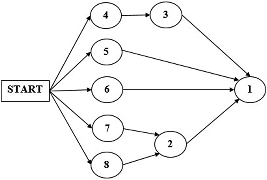
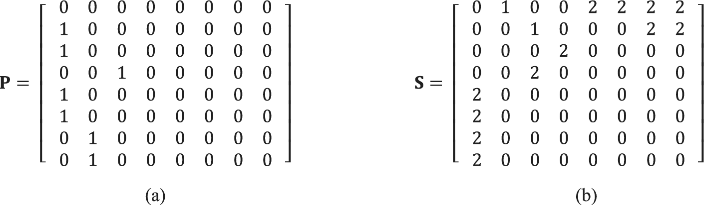
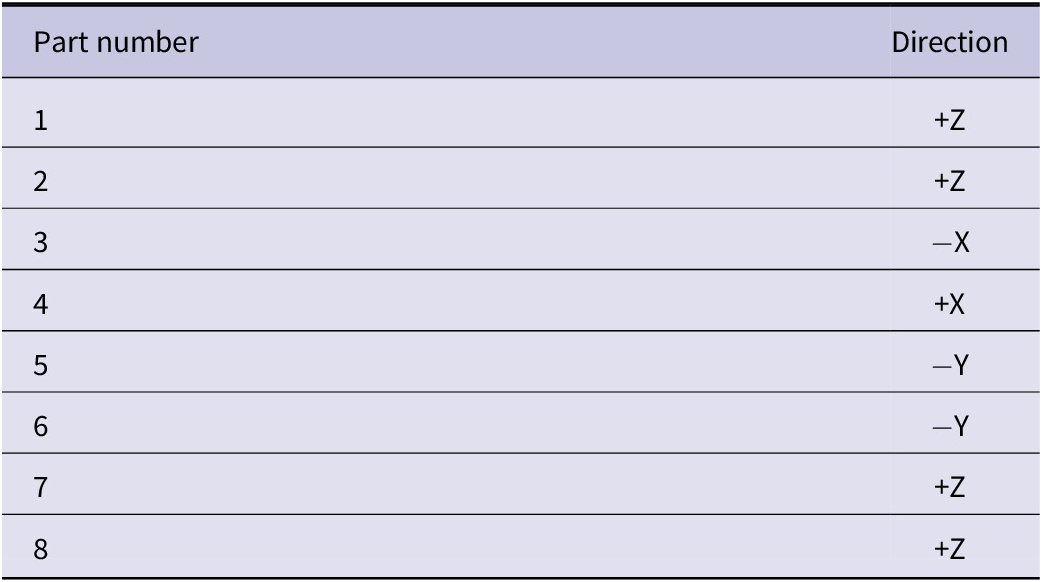
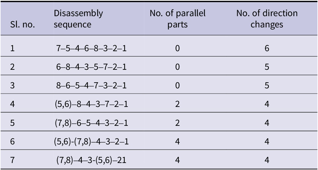
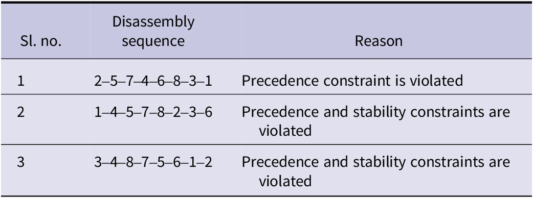
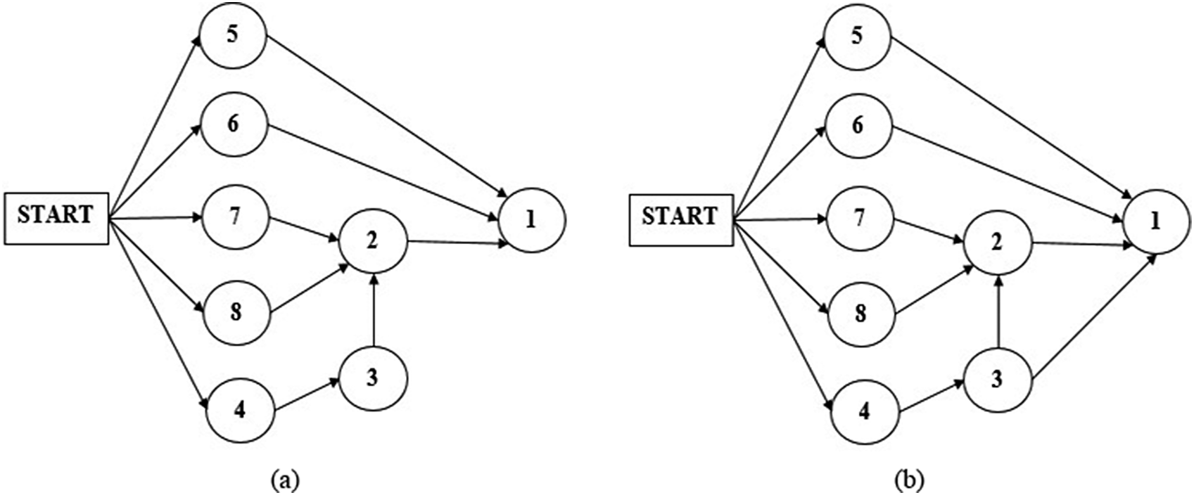




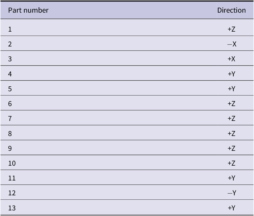
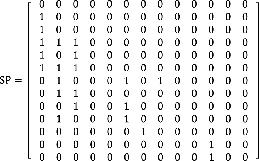


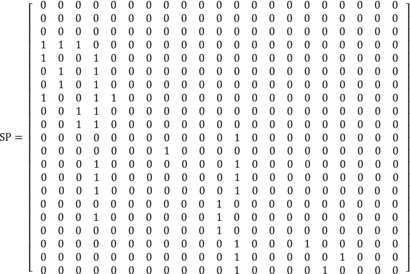
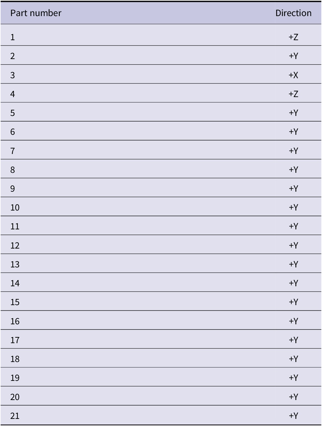


 Open access

