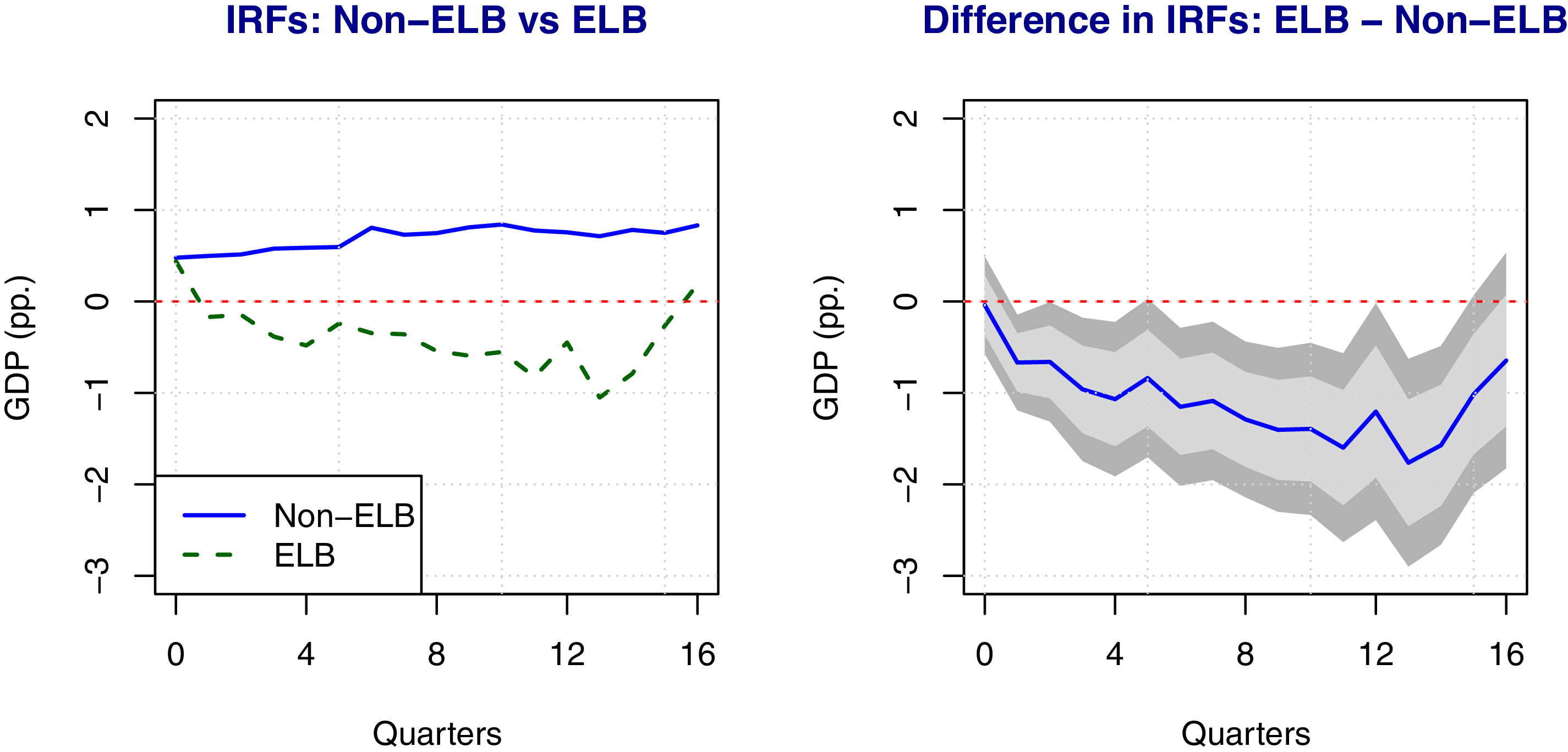
1. Introduction
Productivity shocks are an important source of business cycle fluctuations (Kydland and Prescott, Reference Kydland and Prescott1982; Wang and Wen, Reference Wang and Wen2011; Brinca et al. Reference Brinca, Chari, Kehoe and McGrattan2016). Existing empirical literature argues that positive productivity shocks are estimated to be more expansionary at the effective lower bound (hereafter, ELB) compared to normal times (Garín et al. Reference Garín, Lester and Sims2019). This is in stark contrast to the findings of a basic New Keynesian (hereafter, NK) as well as a medium-scale macro model, which suggests the opposite. A positive supply shock should, in theory, reduce the natural rate of interest. However, this dynamic is likely to change in a framework that does not assume a linear response to productivity shocks, due to the monetary policy channel. When monetary policy is active, an inflation-targeting central bank would respond to a positive supply shock by reducing the nominal rate to track the natural interest rate, thereby stimulating economic activity.Footnote 1 On the contrary, monetary policy operating at the ELB, constrains the central bank’s ability to respond to the same shock by reducing the nominal rate. Consequently, this will increase the real interest rate, and potentially depress economic activity.
This paper empirically tests for differences in the response of the U.S. economy to productivity shocks under different monetary policy regimes, using quarterly data from 1947 to 2022. I follow Klein and Linnemann (Reference Klein and Linnemann2021), and use Fernald (Reference Fernald2014)’s series on the growth rate of utilization and markup-adjusted total factor productivity as an instrument to identify surprise technology shocks in a proxy VAR model.Footnote 2 This is followed by estimating a threshold model where the assumption of linearity is relaxed and the response of the economy is conditional on the monetary policy regime. The impulse response functions are then calculated using the method of local projections à la Jordà (Reference Jordà2005). My results show that productivity shocks are expansionary when monetary policy is active, whereas these shocks tend to be contractionary in the ELB. This indicates that the negative effects of productivity shocks via the monetary policy channel outweigh any favorable effects originating from other mechanisms, when the economy is at the ELB.
A deeper dive into disaggregated data suggests that the nonlinear transmission of productivity shocks around the ELB is primarily driven by the interest-sensitive component of GDP, i.e., private investment. This key result reinforces the role played by the monetary policy channel in changing the propagation of productivity shocks to the U.S. economy. Additionally, I find that the nonlinear transmission of productivity shocks is broad-based, as major macroeconomic indicators on credit, production, labor market, and consumer spending also show a contractionary (expansionary) response in the ELB (non-ELB).
It is worth pointing out that the overlap between the ELB and recessions might cast doubt on the evidence of nonlinearity, as this has the potential to confound my responses associated with each regime.Footnote 3 To ensure that the ELB is not acting as proxy for a slowdown in the economy, I control for recessions in my empirical specification and show that the effect of productivity shocks is not conditional on the state of the business cycle. This is in stark contrast to the literature on fiscal policy (Auerbach and Gorodnichenko, Reference Auerbach and Gorodnichenko2012), monetary policy (Tenreyro and Thwaites, Reference Tenreyro and Thwaites2016), and oil prices (Hwang and Kim, Reference Hwang and Kim2024), which argue the effects of shocks are different in recessions compared to expansions.Footnote 4
My contribution to the literature is threefold. First, examining how the U.S. economy responds differently to productivity shocks at the ELB allows me to reconcile the empirical findings with a medium scale macro model that incorporates capital accumulation and several other frictions (Smets and Wouters, Reference Smets and Wouters2007), as well as a textbook NK model, which has so far been unaddressed. These class of models suggest that productivity shocks will be contractionary at the ELB due to the monetary policy channel. In such a scenario, a positive productivity shock will lower the inflation rate, and result in a rise in the real rate due to the central bank’s inability to pursue conventional expansionary policy, as a result of the ELB constraint. This, in turn, will generate adverse effects for the economy. The absence of a binding constraint in an active monetary policy regime implies that an inflation-targeting central bank would be able to pursue expansionary policy following a positive supply shock and stimulate the economy. Despite the presence of this theoretical mechanism, Garín et al. (Reference Garín, Lester and Sims2019) find no empirical evidence of productivity shocks having contractionary effects at the ELB. This discrepancy results from differences in how productivity shocks are identified and its subsequent incorporation within the local projection specification. The specification in Garín et al. (Reference Garín, Lester and Sims2019) uses utilization-adjusted total-factor productivity (hereafter, TFP) directly as a measure of productivity shock. This approach is problematic because the TFP measure is subject to measurement error, as noted by Kurmann and Sims (Reference Kurmann and Sims2021), and the resulting impulse responses are likely to suffer from attenuation bias (Carriero et al. Reference Carriero, Mumtaz, Theodoridis and Theophilopoulou2015). Identifying the orthogonal productivity shock using utilization-adjusted TFP as an instrument in a proxy VAR is likely to yield unbiased impulse responses, as demonstrated in Carriero et al. (Reference Carriero, Mumtaz, Theodoridis and Theophilopoulou2015).Footnote 5
Second, by analyzing a broad range of macroeconomic indicators, I identify the key driver of the nonlinear transmission of productivity shocks around the ELB. Specifically, I demonstrate that private domestic investment, a major component of GDP, behaves differently, whereas consumption does not.Footnote 6 Third, I extend the general literature highlighting the central role of the ELB in changing the transmission of economic shocks to the U.S. economy. This builds on the fiscal policy (Christiano et al. Reference Christiano, Eichenbaum and Rebelo2011), uncertainty (Plante et al. Reference Plante, Richter and Throckmorton2018), and oil price (Bodenstein et al. Reference Bodenstein, Guerrieri and Gust2013; Datta et al. Reference Datta, Johannsen, Kwon and Vigfusson2021; Sardar and Sharma, Reference Sardar and Sharma2022) literature documenting the nonlinear effects of economic shocks driven by constrained conventional monetary policy. Notably, Wieland (Reference Wieland2019) and Debortoli et al. (Reference Debortoli, Galí and Gambetti2020) show that the ELB does not alter the transmission of macroeconomic shocks and many of the usual rules of economics continue to hold.Footnote 7 In Section 3.6, I show that the diverging results in reference to Debortoli et al. (Reference Debortoli, Galí and Gambetti2020) are driven by differences in the method of shock identification.
The next section outlines the data and empirical framework. Section 3 discusses the empirical results. I present a battery of robustness checks in Section 4, including but not limited to, studying the response of a broad-range of macroeconomic variables, understanding the role of unconventional monetary policy in altering the transmission of productivity shocks, estimating a specification with inflation expectations, and relying on an alternative definition for the Fed’s binding constraints. Section 5 concludes.
2. Data and empirical framework
2.1 Data
I rely on quarterly data for the US economy, with the sample ranging from 1947 Q2 to 2022 Q1. The start period is determined by the availability of Fernald (Reference Fernald2014)’s utilization-adjusted TFP series, while the end period is chosen to capture the most recent ELB episode, from 2020 Q2 to 2022 Q1. The effective Federal Funds Rate (FFR) (
 $i_t$
) is used as the measure of interest rate to identify the monetary policy regime. Specifically,
 $i_t \leq 0.25$
, is classified as the ELB, whereas
 $i_t\gt 0.25$
is defined as the “normal” monetary policy regime (hereafter, non-ELB). It is worth noting that Bernanke and Reinhart (Reference Bernanke and Reinhart2004) and Swanson and Williams (Reference Swanson and Williams2014) present evidence of the Federal Reserve’s binding constraint changing over time, despite the FFR not being close to zero at various time periods before 2007. Consequently, I also rely on alternative thresholds for
 $i_t$
to define monetary policy regimes, and show that my results are unchanged in the robustness section.
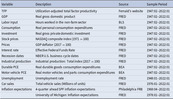
Labor productivity is defined as real GDP per hours worked in the nonfarm business sector.Footnote 8 I consider the response of a broad range of macroeconomic variables to productivity shocks, namely GDP, personal consumption expenditures, private investment, stock prices, and GDP deflator. The GDP deflator is used as the baseline measure of prices, however, the results continue to hold if it is replaced with the PCE price index.Footnote 9 The source and details for all the variables are presented in Table 1. To ensure that the nonlinear transmission of productivity shocks to the U.S. economy is broad-based and not specific to a set of variables, I consider economic indicators such as, industrial production, durable goods consumption expenditures, motor vehicle consumption expenditures, unemployment rate, and total vehicle sales.
Variable names and description

Note: The data sources are FRED: Federal Reserve Economic Database, BLS: Bureau of Labor Statistics, BEA: Bureau of Economic Analysis, and FRB: Federal Reserve Bank.
2.2 Empirical Framework
This section outlines the empirical framework used to identify the structural shock, and estimate its state-dependent effects at and away from the ELB.
2.2.1 Linear model: Proxy VAR
Consider the following reduced-form VAR(p) model:
 \begin{equation} x_t= a + B_1 x_{t-1} + \ldots + B_p x_{t-p} + u_t, \end{equation}
where p represents the lag length,
 $x_t$
is an
 $n \times 1$
vector of endogenous variables,
 $u_t$
is an
 $n \times 1$
vector of reduced-form innovations with the variance-covariance matrix
 $\Sigma$
,
 $a$
is an
 $n \times 1$
vector of constants, and
 $B_1,\ldots ,B_p$
correspond to the
 $n \times n$
coefficient matrices on lag
 $p$
of
 $x_t$
. The reduced-form residuals are a linear function of the orthogonal shocks,
 $\varepsilon _t$
, and can be represented as
 $u_t=S \varepsilon _t$
, where
 $S$
is the structural impact matrix. Without loss of generality, if labor productivity is ordered first in the vector of endogenous variables,
 $x_t$
, the first shock in
 $\varepsilon _t$
will correspond to the surprise productivity shock,
 $\varepsilon _{1,t}$
. My aim is to identify the first column of
 $S$
, which corresponds to the contemporaneous effect of
 $\varepsilon _{1,t}$
on all variables in the system. This identification is done using an external instrument, as outlined in Mertens and Ravn (Reference Mertens and Ravn2013).
I follow Klein and Linnemann (Reference Klein and Linnemann2021), and use Fernald (Reference Fernald2014)’s series on the growth rate of utilization and markup-adjusted total factor productivity as the external instrument to identify the structural productivity shock. For the instrument to be valid, it must be correlated with the shock of interest (
 $\varepsilon _{1,t}$
) and uncorrelated with other structural shocks (
 $\varepsilon _{j,t} \; \forall \; j \neq 1$
) in the VAR system. We present results and a detailed discussion related to the strength and exogeneity of the instrument in Section 3.1. The vector of endogenous variables,
 $x_t$
takes the following form:
 \begin{equation} x_t=\big[prod_t \;\; y_t \;\; c_t \;\; i_t \;\; s_t \;\; \pi _t \;\; ffr_t\big] \end{equation}
Where
 $prod_t$
is labor productivity,
 $y_t$
represents real GDP,
 $c_t$
is real consumption,
 $i_t$
is real gross fixed private investment,
 $s_t$
represents the S&P 500 index,
 $\pi _t$
is the year-on-year change in GDP deflator, and
 $ffr_t$
is the effective Federal Funds Rate. The choice of the S&P 500 index as an endogenous variable is motivated by Beaudry and Portier (Reference Beaudry and Portier2006) and Klein and Linnemann (Reference Klein and Linnemann2021), who argue that stock price movements foreshadow technological innovation. All variables, except the inflation rate and interest rate, are expressed in log levels and specification (1) is estimated with four lags, in line with Klein and Linnemann (Reference Klein and Linnemann2021). Since the variables are expressed in log levels, the impulse response functions from this specification can be interpreted as the cumulative effect of a surprise productivity shock on each variable. It is worth pointing out that the linear model aims to establish a baseline for comparison with the results from my local projections model, discussed in the subsequent section.
2.2.2 Nonlinear model: Local projections
The identified shock is recovered from equation (1), and the state-dependent response of the U.S. economy to productivity shocks around the ELB is estimated using local projections. The orthogonal (exogenous) nature of the productivity shock enables its use in local projections, where the impulse response functions correspond to the slope coefficient generated by regressing the variable of interest on the identified shock at each forecast horizon (
 $h$
). Our implementation closely follows Ramey (Reference Ramey2016), Alloza (Reference Alloza2022), and Adolfsen et al. (Reference Adolfsen, Ferrari Minesso, Mork and Van Robays2024), who use an orthogonal shock identified from a structural VAR model in local projections to estimate the nonlinear effects of a macroeconomic shock.Footnote
10
In that spirit, I specify a threshold model that allows the response of the economy to be conditional on the monetary policy regime. To ensure that my results are not sensitive to how the productivity shock enters the local projections framework, I estimate an alternative empirical specification where the productivity shock is identified in a single step using an instrumental variable approach, and show that the results continue to hold in Section 4.5. My empirical specification, which involves estimating a series of regressions at each horizon
 $h$
from
 $h=0$
to
 $k$
, takes the following form:
 \begin{align} \Delta {x}_{t+h} &=\alpha _{h}+\beta _{h}\varepsilon _{prod,t}+\sum _{l=1}^{n}X^{\prime}_{i,t-l}B_{h,l}+I_{t-1}^{elb}\times \left [\alpha _{h}^{elb}+\beta _{h}^{elb}\varepsilon _{prod,t}+\sum _{l=1}^{n}X^{\prime}_{i,t-l}B_{h,l}^{elb}\right ] \nonumber \\ &\quad +\, I_{t-1}^{rec}\times \left [\alpha _{h}^{rec}+\beta _{h}^{rec}\varepsilon _{prod,t}+\sum _{l=1}^{n}X^{\prime}_{i,t-l}B_{h,l}^{rec}\right ]+u_{t+h}. \end{align}
In equation (3),
 $\Delta {x}_{t+h}$
represents the percentage change in the response variable,
 $x_t$
, in time period,
 $t+h$
,Footnote
11
 $\alpha _h$
is the intercept,
 $\varepsilon _{prod,t}$
represents the productivity shock as identified in Section 2.2.1,
 $X^{\prime}_{i,t-l}$
is the vector of control variables which includes four lags (
 $n=4$
) each of the response variable, productivity shocks and inflation rate. Adding lags to Eq. (3) as controls also allows me to increase the signal-to-noise ratio of productivity shocks by removing the variation explained by past values of the response variable and the shocks. It is worth noting that there is some degree of overlap between the ELB and when the U.S. entered a recession.Footnote
12
Consequently, as a control, the response of the economy is also assumed to be conditional on the state of the business cycle. Thereby, alleviating any concerns that the observed nonlinear response to productivity shocks is driven by recessions, and the ELB is merely acting as a proxy for it.
I follow Ahmed et al. (Reference Ahmed, Borio, Disyatat and Hofmann2024), and introduce nonlinearities in equation (3) through indicator variables,
 $I^{elb}_{t-1}$
and
 $I^{rec}_{t-1}$
.Footnote
13
 $I_{t-1}^{elb}$
is an indicator of the ELB regime, i.e., it takes a value of
 $1$
when
 $i_{t-1} \leq 0.25$
and
 $0$
otherwise. Similarly,
 $I_{t-1}^{rec}$
is
 $1$
when the economy is in a recession and
 $0$
otherwise.Footnote
14
Based on equation (3), the response of the economy to productivity shocks at horizon
 $h$
is given by:
-
•
 $\beta _{h}$
for the non-ELB (
$I_{t-1}^{elb}=0$
) and expansion (
$I_{t-1}^{rec}=0$
)
-
•
$\beta _{h}+\beta _{h}^{elb}$
for the ELB (
$I_{t-1}^{elb}=1$
) and expansion (
$I_{t-1}^{rec}=0$
) -
•
$\beta _{h}+\beta _{h}^{rec}$
for the non-ELB (
$I_{t-1}^{elb}=0$
) and recession (
$I_{t-1}^{rec}=1$
)


The advantage of specification (3) is that it allows me to simultaneously test the role played by monetary policy and the state of the economy in changing the transmission of productivity shocks.Footnote 15 This is done by estimating the cumulative IRFs, and calculating the cumulative difference (hereafter, CD) functions, as in Bachmeier and Keen (Reference Bachmeier and Keen2023). The CD functions, expressed as
 \begin{equation} CD^{\,j}_{t+k}=\sum _{h=0}^k \big(\beta _h+\beta _{h}^{j}\big)-\sum _{h=0}^k (\beta _h), \end{equation}
represent the difference in the cumulative effect of a productivity shock across regimes
 $j \in [elb,rec]$
at horizon,
 $k$
. I am interested in testing whether
 $CD^{\,j}_{t+k}=0$
, where rejecting this hypothesis would imply that the response of the economy to productivity shocks is statistically different in regime
 $j$
.
The confidence bands of the CD functions are calculated following a bootstrap procedure, as outlined in Forni et al. (Reference Forni, Gambetti, Maffei-Faccioli and Sala2024). This approach involves (i) bootstrapping the estimated VAR residuals from Eq. (2) along with the productivity shock,
 $\varepsilon _{prod,t}$
, (ii) using the bootstrapped residuals and shock, along with the estimated coefficients of Eq. (2) to create a new sample, (iii) re-identifying the productivity shock with the new sample, and (iv) computing the CD functions following Eq. (4). Steps (i)–(iv) are repeated 1,000 times to construct confidence bands of the CD functions. This procedure allows me to account for the estimation uncertainty associated with a generated regressor, i.e., productivity shock.
3. Empirical results
3.1 Instrument strength and exogeneity
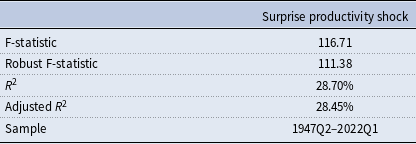
I begin by presenting results on the strength and relevance of the instrument in Table 2. This is done by utilizing the F-statistic generated from the first-stage regression (Montiel Olea et al. Reference Montiel Olea, Stock and Watson2021; Känzig, Reference Känzig2021), where the labor productivity residual from the VAR is regressed on the instrument, i.e., utilization-adjusted TFP. The F-statistic of 116.71 suggests weak instrument is unlikely to be a problem, as it is above the threshold value of 10. The robust F-statistic, which allows for heteroskedasticity corresponds to 111.38, and approximately 28% of the variation in the reduced-form productivity residual is explained by the instrument. Overall, this evidence reinforces the validity and strength of the instrument.
Instrument relevance

Note: The table shows the results for the first-stage regression of the labor productivity residual on Fernald (Reference Fernald2014)’s series on the growth rate of utilization and markup-adjusted total factor productivity. F-statistics above 10 indicate strong instruments. Robust F-statistics allow for heteroskedasticity.
To illustrate the exogeneity of the external instrument, I employ two complementary approaches: one based on principal components analysis à la Forni and Gambetti (Reference Forni and Gambetti2014), and another that tests the predictability of the instrument with respect to other Wold residuals in the VAR system, i.e., Eq. (2). The former approach involves utilizing a data set,
 $x_t^*$
, to capture all the relevant macroeconomic information, and computing the first
 $P$
principal components. This is followed by performing a Granger causality test to see whether utilization-adjusted TFP,
 $z_t$
, is Granger caused by the extracted principal components. Failing to reject the null of no Granger causality implies that the external instrument is exogenous, thus making it a safe choice to use in a proxy VAR model to identify the productivity shock.
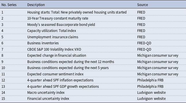
The forward-looking variables, utilized to conduct the test outlined in Table 3, are meant to capture the forward-looking nature of the economy.Footnote
16
This include measures of economic activity (housing starts, capacity utilization, business inventories), labor market conditions (unemployment insurance claims), credit and interest rate expectations (Treasury and corporate bond yields), market sentiment and uncertainty, as well as survey-based expectations of the state of the economy. Table 4 reports results of the Granger causality tests for the first five PCs. The null hypothesis states that the external instrument
 $z_t$
is not Granger-caused by the first
 $k$
principal components (
 $PC=k$
) extracted from
 $x_t^*$
. The choice of five principal components is chosen because these capture a significant amount of variation in
 $x_t^*$
, i.e., 91.5%, while also maintaining parsimony. It is worth noting that there is no strict upper bound on the number of PCs that can be used for this test; however, including too many factors risks undermining parsimony and over-fitting, as later components often capture idiosyncratic noise rather than meaningful common variation. The lag length of four is selected to ensure consistency with the empirical specifications in Eqs. (2) and (3).Footnote
17
Forward-looking variables for instrument exogeneity test

Note: Data sources are FRED: Federal Reserve Economic Data, FRED-QD: FRED Quarterly Database, FRB: Federal Reserve Bank.
Instrument and shock exogeneity test

Note: This table shows the F-statistics and the p-values for each regression including up to 4 lags of the first
 $k$
principal components (PCs). The null hypothesis is no Granger causality.
The columns in Table 4 that fall under the category,
 $z_t$
, present corresponding
 $p$
-values and F-statistics for the predictability of the instrument with respect to PCs extracted from
 $x_t^*$
. In all instances, the reported
 $p$
-values are in excess of 0.10, which suggests that I fail to reject the null hypothesis of no Granger causality (lack of predictability) at the 10% level. These findings point to instrument exogeneity.
In a related exercise, I also test the orthogonality of the identified productivity shock. The statistics reported under
 $\varepsilon _{prod,t}$
in Table 4 correspond to predictability tests of the identified shock with respect to PCs extracted from
 $x_t^*$
. The uniformly high
 $p$
-values indicate a failure to reject the null of no predictability, providing evidence in favor of partial invertibility of the identified shock. In the robustness section, I replicate this exercise using the McCracken and Ng (Reference McCracken and Ng2016) dataset (FRED-QD), and again find evidence in favor of shock orthogonality. This suggests that the productivity shock remains partially invertible even when a richer macroeconomic information set is employed.
One of the conditions for instrument validity is that it should be plausibly exogenous with respect to other structural shocks in the VAR system. To assess the plausibility of the exclusion restriction, I conduct a test in the spirit of Forni et al. (Reference Forni, Franconi, Gambetti and Sala2025).Footnote
18
If the instrument is contaminated, then it is likely to be a function of current and future VAR residuals of the non-target variables. This test involves regressing the instrument on the current and first
 $r$
leads of the Wold residuals (
 $\hat {e}_{j,t+k}$
) for the non-target variable,
 $j=(y_t,\;c_t,\;i_t,\;s_t,\;\pi _t,\;ffr_t)$
, recovered from the baseline VAR model, i.e., Eq. (2). The test takes the following form:
 \begin{equation} z_t=\sum ^r_{k=0}\lambda ^{\prime}_k \hat {e}_{j,t+k}+\eta _t. \end{equation}
Formally, the instrument exogeneity test is an F-test for the significance of the
 $r$
leads, with the null hypothesis stating
 $H_0=\lambda _0=\lambda _1=\ldots =\lambda _r=0$
against the alternative that at least one of
 $\lambda _k\neq 0$
. This allows me to analyze whether the
 $z_t$
is predicted by other non-target shocks. If I reject the null, that would suggest that other shocks in the VAR system have predictive power over the instrument, and as such one cannot claim that it is exogenous, bringing into question the validity of the identified productivity shock,
 $\varepsilon _{prod,t}$
. The corresponding statistics for
 $H_0$
from Eq. (5) are reported in Table 5. In all instances, the high
 $p$
-values and low F-statistics indicate that the instrument is uncorrelated with other structural shocks, and thus points to its exogeneity which makes it a safe choice to use in a proxy VAR setting to identify productivity shocks.
Instrument exogeneity test with respect to non-target shocks

Note: The table reports the p-value and the F-statistic for the null of instrument exogeneity against the alternative that other shocks in the VAR system hold predictive power for
 $z_t$
.
3.2 Linear model: Proxy VAR
The cumulative impulse responses of the U.S. economy to a
 $1\%$
productivity shock from the linear proxy VAR model are presented in Figure 1. My results indicate that a positive productivity shock reduces inflationary pressures which prompts an inflation-targeting Federal Reserve to reduce the nominal interest rate.Footnote
19
As long as the decline in the nominal rate is more than the decline in the inflation rate, a productivity shock will lower the ex-post real rate of interest, and stimulate the economy. The shock response of the ex-post real interest rate can be read off as the difference between the cumulative responses of the FFR and inflation. Specifically, I find that for the first 4 quarters following the shock, the negative response of the Federal Funds Rate is stronger than that of the inflation rate, thereby suggesting a decline in the real rate of interest. This stimulates the economy, as indicated by the expansionary responses of output, consumption, and investment. Asset prices, as measured by the S&P 500 index, also rise following the shock. The impulse responses are statistically significant at the 90% confidence level. The key takeaway from this section is that the monetary policy channel plays a central role in influencing the transmission of productivity shocks.
Cumulative response of U.S. economy to productivity shocks.
Note: The solid lines represent the cumulative response of the U.S. economy to a one percent surprise productivity shock. The light and dark gray shaded regions represent the 68% and 90% confidence intervals, respectively.

3.3 Nonlinear model: Local projections
There is reason to believe that the effects of productivity shocks are different across monetary policy regimes, as stated earlier. This motivates me to estimate a threshold model, and the cumulative impulse responses are presented in Figure 2. Although productivity shocks are expansionary on impact across both monetary policy regimes, the long-run effects differ significantly. Specifically, a one-standard deviation shock in the non-ELB regime leads to an expansion of the economy with the response of output peaking at 0.82 pp. after ten quarters. The same shock in the ELB generates a contraction, with output declining by as much as 0.67 pp. after eight quarters. In the long-run, however, the economy rebounds in the ELB, and the cumulative effect converges towards zero. The difference in response across both regimes, expressed as the CD function, is statistically significant for all forecast horizons, except
 $k=0$
. The results in the third and fourth columns of Figure 2 shows a reduction in inflationary pressures following a productivity shock across both regimes. This decline, however, is stronger for the ELB as opposed to the non-ELB regime. The difference in response, however, is not statistically significant.
Cumulative response of GDP and inflation to productivity shocks around the ELB.
Note: The first and third panels represent the cumulative response of GDP and inflation to a one-standard deviation surprise productivity shock. The second and fourth panels are the corresponding difference in response between the ELB and non-ELB regimes, expressed as the cumulative difference functions. The light and dark gray shaded regions represent the 68% and 90% bootstrapped confidence intervals, respectively.

I hypothesize that the nonlinear response of output is driven by the state-dependent shock response of the real rate of interest at and away from the ELB. As demonstrated, inflation responds negatively to productivity shocks across both regimes. However, when monetary policy is active, the central bank responds to the easing of inflationary pressures by lowering the nominal rate sufficiently to track the natural rate of interest, thereby stimulating output and investment, as shown in Figure 2. At the ELB, however, the central bank’s inability to adjust the policy rate implies that real interest rates rise relative to the natural rate, leading to a contraction, as illustrated in Figure 2. These results extend the general literature documenting how the response of the economy to a macroeconomic shock is different at the ELB.
These empirical findings are consistent with the predictions of a textbook NK model when the ELB is binding, as well as a medium-scale macro model (Smets and Wouters, Reference Smets and Wouters2007), as shown by Garín et al. (Reference Garín, Lester and Sims2019). These class of models generate nonlinear effects of productivity shocks at the ELB under capital accumulation, investment adjustment costs, variable capital utilization, nominal price and wage rigidities with partial indexation, and habit formation.Footnote 20 Importantly, these benchmark frameworks abstract from (i) financial frictions, and (ii) central bank credit or balance-sheet policy.
For the purpose of exposition, it is useful to discuss the implications of incorporating financial frictions and central bank credit policies for the nonlinear effects of a productivity shocks in a theoretical setting. The discussion below is intended to provide a conceptual overview of how the inclusion of these features would be expected to alter the results, with a formal evaluation left to future work. In particular, the presence of financial frictions and central bank credit policies would likely modify the propagation of productivity shocks through two distinct channels.
First, introducing financial frictions will amplify the effects of productivity (technology) shocks, as demonstrated by Gertler and Karadi (Reference Gertler and Karadi2011). In models with intermediary balance-sheet constraints and an endogenous risk premium, the amplification of these shocks is a product of the enhanced response of investment (Gertler and Karadi, Reference Gertler and Karadi2011). Away from the ELB, a positive productivity shock raises investment and asset prices, which improves the intermediary balance sheets and lowers risk-adjusted premium. This channel will unleash a credit-investment boom that magnifies the expansion. When the ELB binds and under the assumption that the central bank does not provide credit, dis-inflationary pressures following a productivity shock raise real rates relative to the natural rate and reduce investment along with asset prices. This creates a deterioration in the balance sheets, which increases the premium. The increase in the cost of acquiring capital further reduces demand for capital by non-financial firms, which will likely trigger a sharper contraction than in frictionless models. Because the risk-adjusted premium is zero by assumption in baseline NK and medium-scale macro models (Smets and Wouters, Reference Smets and Wouters2007), but endogenous under financial frictions, the investment-driven nonlinearity observed in the data could plausibly be stronger in a financially constrained economy.
Second, frameworks that incorporate financial frictions (Gertler and Karadi, Reference Gertler and Karadi2011; Gertler and Kiyotaki, Reference Gertler and Kiyotaki2015), also allow for central banks to provide credit to financial intermediaries when conventional monetary policy is constrained. In this scenario, unconventional policy tools (such as, credit policies and large-scale asset purchases) can partially offset the contractionary effects of productivity shocks during the ELB period by stabilizing intermediary balance sheets and compressing risk premia. In other words, following a productivity shock, the Fed can counteract upward pressure on the real interest rate relative to the natural rate by engaging in QE. Consequently, the contractionary effects of productivity shocks at the ELB may be attenuated in environments where credit policy supports investment by easing financing conditions. While constructing a full financial-intermediation and central-bank balance-sheet block lies beyond the scope of this paper, this mechanism finds empirical support in the robustness analysis. In particular, the U.S. economy’s response to productivity shocks during periods of unconventional monetary policy exhibits a more muted adverse effect compared to the results presented in Figures 2 and 3. Nevertheless, the difference in responses across regimes remains statistically significant. A detailed explanation of this mechanism follows in Section 4.2.
3.4 Comment on the validity of local projections estimates
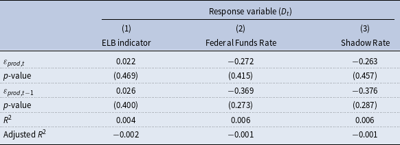
Gonçalves et al. (Reference Gonçalves, Herrera, Kilian and Pesavento2024) show that the inference from local projections might be invalid in instances when the state of the economy is endogenous with respect to the shock of interest. Specifically, they show that the conditional average response, which is what LP estimates, is not consistent and subject to bias in such a scenario. To ensure that the monetary policy regime is exogenous to productivity shocks, I conduct a state-exogeneity test following Adolfsen et al. (Reference Adolfsen, Ferrari Minesso, Mork and Van Robays2024). This test involves regressing the conditioning variable on the orthogonal shock, and testing the significance of the slope coefficients. I estimate regression (6), and report the corresponding estimates in Table 3.
 \begin{equation} D_t=\alpha +\beta _0 \varepsilon _{prod,t} +\beta _1 \varepsilon _{prod,t-1}+v_t \end{equation}
Where
 $D_t$
is the ELB indicator variable,
 $I^{elb}_t$
, FFR, or Shadow Rate,
 $\varepsilon _{prod,t}$
is the productivity shock, and
 $v_t$
is the residual. In addition to the FFR, I capture the stance of monetary policy using the Shadow Rate proposed by Wu and Xia (Reference Wu and Xia2016). Unlike the observed FFR, the Shadow Rate is not constrained by the ELB of 0%, and can take on negative values during periods when the Federal Reserve relies on unconventional monetary policy to stimulate the economy. This feature allows me to assess whether productivity shocks can explain fluctuations in the monetary policy stance during the ELB period.
Results from the first column of Table 6 suggest that a 1% productivity shock increases the probability of the ELB regime by a mere 2%. The reported p-value suggests that the effect isn’t statistically significant either. Similarly, a positive productivity shock is associated with a decrease in the interest rate, but the p-value of 0.415 indicates that this effect is not statistically significant either. The estimates for column (3) can be interpreted similarly. The low
 $R^2$
for all specifications reinforces the point that the state of the economy (monetary policy regime) is not endogenous, as the orthogonal productivity shocks explain negligible variation in the conditioning variables. Overall, the presented evidence indicates that the monetary policy regime is exogenous with respect to productivity shocks, which justifies the use of LP to estimate the state-dependent impulse response functions.
Regime exogeneity test

Note: This table represents the point estimates and regression statistics from specification (6). Shadow rate corresponds to the Shadow Federal Funds Rate proposed by Wu and Xia (Reference Wu and Xia2016).
3.5 Propagation channel
The previous section highlights the role played by the monetary policy channel in altering the transmission of productivity shocks to the U.S. economy. To better understand why output behaves differently, I analyze the response of its two major components, i.e., personal consumption and private investment, around the ELB. If the monetary policy channel is indeed responsible for this change, one would expect private investment to exhibit evidence of strong nonlinearities to productivity gains in the ELB, due to its higher degree of sensitivity to changes in the cost of borrowing (David and Gurio, Reference David and Gurio2023).
Column (1) in Figure 3 suggests that personal consumption expenditures increase following a productivity shock in both the non-ELB and ELB regimes. Specifically, a one standard productivity shock generates cumulative increases of 0.81 pp. in the non-ELB, compared to 0.25 pp. in the ELB after two years. However, the difference in response is not statistically significant, as zero lies within the 90% confidence bands for all forecast horizons, as shown in column (2) of Figure 3. The cumulative responses across both regimes suggest that productivity shocks have the ability to stimulate consumer spending through the wealth channel, even if monetary policy is constrained by the ELB. Specifically, improved productive capacity will generate a rise in asset prices, which in turn will increase consumer demand (Ludvigson et al. Reference Ludvigson, Steindel and Lettau2002). My results indicate the presence of this mechanism across both regimes, with the caveat that the response of consumer spending is slightly weaker in the ELB compared to the non-ELB regime. This finding shows that the adverse effects of productivity shocks originating from the monetary policy channel may be more than offset by the wealth effect, which generates favorable effects for consumption in response to productivity gains.
Cumulative response of consumption and investment to productivity shocks around the ELB.
Note: The first and third panels represent the cumulative response of consumption and private investment to a one-standard deviation surprise productivity shock. The second and fourth panels are the corresponding difference in response between the ELB and non-ELB regimes, expressed as the cumulative difference functions. The light and dark gray shaded regions represent the 68% and 90% confidence intervals, respectively.

Interestingly, I find that the shock response of private investment is substantially different at the ELB. A productivity shock in the active monetary policy regime will be followed by a rise in investment, as firms anticipate higher marginal returns on capital and improved future profitability. The same shock in the ELB, however, generates a fall in investment. The difference in response across both regimes is also statistically significant at all forecast horizons, as demonstrated in column (4) of Figure 3. Specifically, I find that a favorable productivity shock generates a cumulative increase of 1.45 pp. over a 1-year horizon during the non-ELB regime, while the corresponding response at the ELB is −1.79 pp.
Traditionally, a favorable productivity shock would be expected to boost the marginal product of capital, and encourage firms to invest in new technologies and capital goods. However, this decision is likely to be influenced by factors such as credit conditions and borrowing costs. When monetary policy is active, a decrease in the inflation rate following a productivity shock, as observed in Figure 2, could potentially be matched by a more accommodative monetary policy stance. This, in turn, will reduce the real rate of interest compared to the scenario in which the Fed does not respond at all. The reduced cost of borrowing in real terms will incentivize firms to finance their investment through the acquisition of credit and loans, and translate into higher investment. This key mechanism explains the positive response of private investment to productivity shocks in the non-ELB regime. Meanwhile, the negative response of investment to productivity shocks in the ELB is influenced by the Fed’s inability to use conventional monetary policy to respond to a decline in inflation. Consequently, a favorable productivity shock in the ELB will increase the real interest rate and discourage firms to borrow, potentially hampering investment.
Cumulative response of private non-financial sector credit (inflation-adjusted) to productivity shocks around the ELB.
Note: The left panel represents the cumulative response of private sector credit to a one-standard deviation surprise productivity shock, and the right panel is the difference in response between the ELB and non-ELB regimes, expressed as the cumulative difference functions. The light and dark gray shaded regions represent the 68% and 90% bootstrapped confidence intervals, respectively.

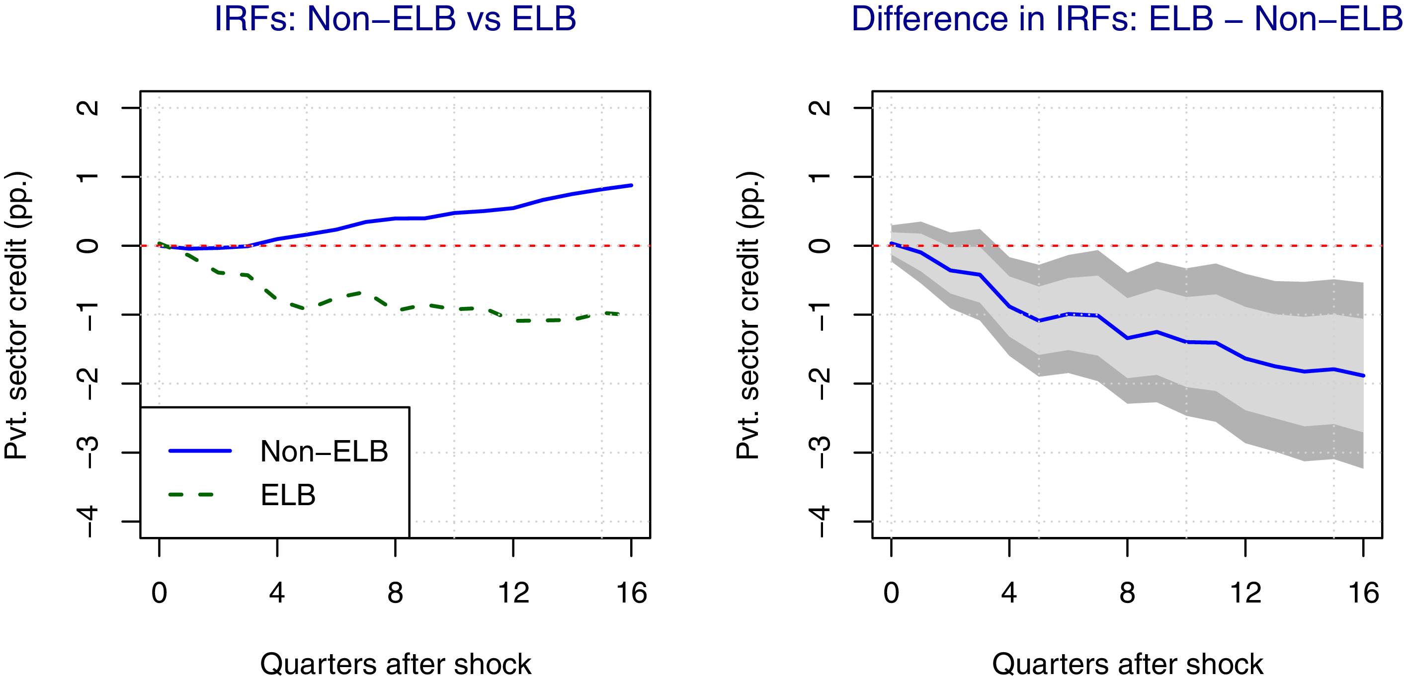
To further validate this potential mechanism at play, I examine whether credit extended by the U.S. banking sector to private non-financial sector (inflation-adjusted) responds differently to productivity shocks in Figure 4.Footnote 21 Private sector credit is a key indicator for understanding the nonlinear transmission of productivity shocks, as it provides insights into how firm’s borrowing behavior could be influenced through changes in the real cost of borrowing. It should be noted that this credit metric only includes funds acquired through loans and debt securities by the private non-financial sector, defined as firms primarily engaged in producing market goods or non-financial services.Footnote 22 Qualitatively, I find that the response of private sector credit to productivity shocks closely mirrors that of private investment. The results indicate that a productivity shock in the non-ELB will be followed by a rise in credit to the private sector, albeit with a slight delay. The cumulative response at the 2- and 4-year horizons correspond to 0.41 and 0.89 pp., respectively. This rise in credit demand subsequently generates an increase in private investment. In contrast, a productivity shock at the ELB leads to an contemporaneous decline of 0.20 pp. in credit to the private sector. This effect intensifies over time, with the 2-year and 4-year responses amounting to −0.81 and −1.64 pp, respectively. This decline in credit, despite improved profitability and higher marginal returns on capital, suggest that the rise in real rates driven by productivity shocks in the ELB discourages firms from borrowing, ultimately translating into a decline in investment.
The findings from this section highlight that when monetary policy is active, the Fed can effectively respond to productivity shocks by adjusting the nominal rate, and facilitate credit expansion and higher investment. On the contrary, the ELB constrains the Fed’s ability to pursue conventional expansionary policy, causing productivity shocks to have contractionary effects on both credit and investment. Overall, these findings lend credence to the claim made earlier in the paper about the monetary policy channel playing a pivotal role in altering the transmission of productivity shocks to the U.S. economy. This builds on the findings of Bodenstein et al. (Reference Bodenstein, Guerrieri and Gust2013), Miyamoto et al. (Reference Miyamoto, Nguyen and Sergeyev2023), and Sardar and Qureshi (Reference Sardar and Qureshi2024), who present similar evidence in the context of oil price shocks.Footnote 23 Moreover, these results also reinforce the point made by Eggertsson and Woodford (Reference Eggertsson and Woodford2003), who suggest that the efficacy of monetary policy in stimulating demand is weaker at the ELB.
3.6 Discrepancies relative to other work
Notably, the results I present in Figure 2 are in stark contrast to the findings of Garín et al. (Reference Garín, Lester and Sims2019) and Debortoli et al. (Reference Debortoli, Galí and Gambetti2020), with the former concluding that productivity shocks are more expansionary at the ELB and the latter showing that the monetary policy regime does not alter the transmission of these shocks. In what follows, I argue that the diverging results are driven by differences in the methods of shock identification.
The discrepancy in reference to Garín et al. (Reference Garín, Lester and Sims2019) arises from differences in the definition of productivity shocks and the way utilization-adjusted TFP is incorporated into the local projection specification. Specifically, Garín et al. (Reference Garín, Lester and Sims2019) equate productivity shocks with Fernald (Reference Fernald2014)’s utilization-adjusted TFP, which pose a major empirical challenge. As noted in Fernald (Reference Fernald2014) and Kurmann and Sims (Reference Kurmann and Sims2021), the TFP estimates are prone to measurement error, leading to potential attenuation bias in the impulse response functions (Carriero et al. Reference Carriero, Mumtaz, Theodoridis and Theophilopoulou2015). The use of utilization-adjusted TFP as an instrument within a proxy VAR allows me to address any potential endogeneity concerns by isolating variation in productivity driven by TFP, but unrelated to factors such as inflation, consumption, investment, and stock prices. Furthermore, this approach mitigates the impact of measurement error, as TFP does not enter the system of equations directly, but is used instead as an instrument. This allows one to filter out the noise and mute the attenuation bias (Carriero et al. Reference Carriero, Mumtaz, Theodoridis and Theophilopoulou2015). Consequently, the resulting IRFs will be close to the true underlying responses.Footnote 24
On the other hand, Debortoli et al. (Reference Debortoli, Galí and Gambetti2020) find no evidence that the ELB alters the transmission of productivity shocks. Their results are derived from a TVP-VAR model in which the productivity (technology) shock is identified following Galí (Reference Galí1999), i.e., the technology shock is assumed to be the only shock with a permanent effect on labor productivity. This long-run restriction has faced growing scrutiny, as noted by Uhlig (Reference Uhlig2004), due to its inability to cleanly identify productivity shocks. Additionally, the TVP-VAR specification excludes forward-looking variables that capture agents’ information about technology (such as stock prices). As emphasized by Forni and Gambetti (Reference Forni and Gambetti2014), this is critical because omitting stock prices when identifying productivity shocks can generate an information deficiency in the VAR.Footnote 25 As a result, the identified productivity shocks may fail to be orthogonal.
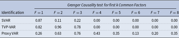
To test the validity of the productivity shocks identified using alternative strategies, namely, a linear SVAR and a TVP-VAR that impose the long-run restriction of Galí (Reference Galí1999), and a proxy VAR that uses utilization-adjusted TFP as an external instrument, I follow the orthogonality test proposed by Mori and Peersman (Reference Mori and Peersman2024).Footnote
26
Specifically, this test involves extracting the first eight common factors from the large quarterly database of McCracken and Ng (Reference McCracken and Ng2016), and testing whether these hold any predictive power over the identified shocks.Footnote
27
Failure to reject the null of no Granger causality points to information sufficiency and orthogonality (exogeneity) of the shock. The results in Table 7 show that the common factors identified in McCracken and Ng (Reference McCracken and Ng2016) jointly Granger-cause the productivity shocks recovered from models that exclude stock prices and impose the long-run restriction, i.e., linear SVAR and TVP-VAR. The low
 $p$
-values for
 $F\geq 4$
implies that we reject the null of orthogonality. This indicates informational insufficiency in these specifications, and suggests that the resulting shocks are not orthogonal to past macroeconomic data. The third row reports the
 $p$
-values of the Granger causality test for the shock identified from a proxy VAR. In this case, the shock is not Granger-caused. Hence, the choice of identification method may help explain the diverging results between this paper and Debortoli et al. (Reference Debortoli, Galí and Gambetti2020).
Exogeneity tests for productivity shocks across identification strategies

Note: This table shows the p-values for each Granger causality test which includes 4 lags of the first k common factors (
 $F=k$
). The null hypothesis states that productivity shocks are not jointly Granger caused by the common factors.
As a robustness check, I also estimate a TVP-VAR model with stochastic volatility in which the productivity shock is identified recursively. Let
 $x_t$
denote the vector of endogenous variables, comprising labor productivity, output, interest rate, inflation, and stock prices. The evolution of
 $x_t$
is described by a TVP-VAR model and takes the form:
 \begin{equation} x_t = a_{t} + B_{1,t} x_{t-1} + B_{2,t} x_{t-2} + \cdots + A_{p,t} x_{t-p} + u_t, \end{equation}
where
 $a_t$
is a vector of time-varying intercepts,
 $B_{i,t}$
are matrices of time-varying autoregressive coefficients, and
 $u_t$
is a vector of reduced-form innovations with time-varying covariance matrix
 $\Sigma _t$
. The reduced-form shocks
 $u_t$
are assumed to be a linear transformation of the structural shocks
 $\varepsilon _t$
,
 \begin{equation} u_t = S_t \varepsilon _t,\qquad S_t S_t^{\prime} = \Sigma _t, \end{equation}
where
 $S_t$
is a lower-triangular contemporaneous-impact matrix with ones on the diagonal, imposing a recursive identification scheme with productivity ordered first. The estimation for Eq. (7) follows Primiceri (Reference Primiceri2005) and Nakajima (Reference Nakajima2011), where all time-varying parameters
 $(a_t, B_{i,t}, S_t, \Sigma _t)$
evolve according to random walks, and the TVP-VAR is estimated via MCMC.Footnote
28
In each iteration, I draw the full sequence of time-varying parameters over the sample period, recover the structural shocks
 $\varepsilon _t$
from the relation
 $u_t = S_t \varepsilon _t$
, and compute the impulse responses to a one-standard deviation productivity shock. The IRFs correspond to the averages of the estimated responses for the ELB and non-ELB periods.Footnote
29
To avoid potential confounding nonlinearities associated with recessionary episodes, which overlap with both the ELB and non-ELB regimes, I exclude IRFs corresponding to those quarters from the regime-specific averages.
Cumulative response of macroeconomic variables to productivity shocks around the ELB estimated using a TVP-VAR model.
Note: This figure represents the cumulative response and the difference in response between the ELB and non-ELB regimes to a one-standard deviation surprise productivity shock. The shaded regions represent the 90% confidence intervals.

Figure 5 corresponds to the IRFs and CD functions generated using a TVP-VAR model. The response of output in the second column suggests that productivity shocks are more expansionary in the non-ELB compared to the ELB, which reinforces the state-dependent effects found in the preceding section. The difference in response, plotted in the second row, is also statistically significant. It is worth noting that despite the initial size of the productivity shock being the same across both monetary policy regimes, there is slight variation in the persistence. Specifically, shocks that occur in the ELB have a slightly stronger effect on productivity than those that occur in non-ELB periods. To the extent that this mechanism influences our results, it will introduce a slight bias against finding nonlinearity, as scaling the output response in proportion to productivity would mechanically produce an even larger expansion in the non-ELB period.
Overall, the results in this section suggest that the divergence from Debortoli et al. (Reference Debortoli, Galí and Gambetti2020) may potentially stem from the shock identification method. The proxy VAR represents an improvement due to its data-driven nature, as it identifies the shock using an external instrument rather than imposing zero restrictions. Moreover, including stock prices in the model helps mitigate the information deficiency in VAR models and produce productivity shocks that are orthogonal in nature.
4. Sensitivity analysis and extensions
This section presents a battery of sensitivity checks and extensions. This includes documenting how the nonlinear transmission of productivity shocks is broad-based by analyzing a set of variables related to production, sales, and labor market. In addition, I also show that my results are robust in alternative empirical specifications, which strengthens the credibility of my baseline estimates in the preceding section.
4.1 Response of other macroeconomic variables
The preceding section highlights the role played by the monetary policy channel in changing the propagation of productivity shocks to the U.S. economy. To reinforce how this state-dependent transmission is broad-based and not confined to aggregate variables like GDP and investment, I consider a range of disaggregated macro indicators, namely, car sales, durable consumption expenditures, motor vehicle spending, industrial production, and unemployment rate. All variables, barring the unemployment rate, which is measured in levels, are expressed as quarterly growth rates. The choice of variables such as car sales and spending on big-ticket items (namely, durable goods and motor vehicles), is dictated by their higher degree of elasticity and responsiveness to monetary policy. These consumption categories respond to changes in interest rates through the credit channel, as increases in the real cost of borrowing result in a decline in the relative demand of bank consumer loans, which in turn produces a decrease in real consumption (Ludvigson, Reference Ludvigson1998). Although total consumption exhibits a cumulative increase in both regimes, as shown in Figure 3, these results should be interpreted with caution. One potential concern is that the negative implications of productivity shocks on overall consumption through changes in the real rate may be obscured by the muted response of services and nondurable goods, which are generally less sensitive to the credit channel.
Cumulative response of macroeconomic variables to productivity shocks around the ELB.
Note: This figure represents the cumulative response and the difference in response between the ELB and non-ELB regimes of various macroeconomic variables to a one-standard deviation surprise productivity shock. The light and dark gray shaded regions represent the 68% and 90% confidence intervals, respectively.

The cumulative IRFs in Figure 6 indicate the presence of nonlinearities in the response of all variables to productivity shocks across each type of monetary policy regime, consistent with my baseline estimates. Specifically, car sales increase by up to 6.37 pp. 11 quarters after the shock in the non-ELB, whereas the same shock in the ELB generates a cumulative decline across all time periods. Motor vehicle and durable goods spending, which has data availability going back to 1947 unlike car sales, show a positive (negative) response to productivity shocks in the non-ELB (ELB). Even though overall consumption increases across both regimes, there is significant heterogeneity in the response of each disaggregated category. Thus, suggesting that the expansionary consumption responses in Figure 3 are primarily driven by non-durables and services, and not durables.
Industrial production increases on impact following a shock in the non-ELB, with the effect peaking after 9 quarters at 1.10 pp. The corresponding response in the non-ELB regime amounts to −2.60 pp. Additionally, the unemployment rate generates a cumulative decline (increase) following a shock in the non-ELB (ELB). The difference in response, as measured by the cumulative difference functions, are statistically significant at various forecast horizons for all the variables under consideration. Overall, the results in this section highlight that the state-dependent effects of productivity shocks are fairly broad-based and validate the findings in the preceding section.
4.2 Role of unconventional monetary policy
The baseline model identifies monetary policy regimes using the effective FFR, which is constrained by the effective lower bound. When the economy entered the ELB, the Federal Reserve deployed large-scale balance sheet measures and other unconventional monetary policy tools to provide additional stimulus. This indicates that although the conventional policy rate was constrained, monetary policy capacity was not fully exhausted. The availability of alternative policy instruments implies that the ELB did not necessarily preclude the favorable transmission of productivity shocks, as the Federal Reserve retained other tools to support the U.S. economy.
To assess the robustness of my results, and also analyze how the state-dependent transmission observed in the preceding section is affected by unconventional monetary policy, I redefine the monetary policy regime using the Shadow Rate (
 $SR_t$
) of Wu and Xia (Reference Wu and Xia2016). As stated in Section 3.4, the Shadow Rate is not bounded by zero and takes on negative values when the Fed engaged in Quantitative Easing (QE). Consequently, the threshold is defined as:
 \begin{equation} I^{QE}_t = \left \{ \begin{array}{ll} 1 &\quad \text{if } SR_t \lt 0, \\[6pt] 0 &\quad \text{otherwise}. \end{array} \right . \end{equation}
Cumulative response of GDP and investment to productivity shocks across shadow rate regimes.
Note: The first and third panels represent the cumulative response of GDP and investment to a one-standard deviation surprise productivity shock. The second and fourth panels are the corresponding difference in response across the shadow rate regimes, expressed as the cumulative difference functions. The light and dark gray shaded regions represent the 68% and 90% bootstrapped confidence intervals, respectively.

This is followed by re-estimating Eq. (3) after replacing
 $I_t^{elb}$
with
 $I_t^{QE}$
, and computing the CD functions. The results, presented in Figure 7, suggest that the conditional effects of productivity shocks continue to persist even after accounting for the Fed’s ability to engage in QE. One key difference, however, is that productivity shocks are now expansionary across both regimes, with the caveat that the effects are stronger when
 $SR_t\gt 0$
. This suggests that the Fed is able to partially mitigate the adverse effects of favorable productivity shocks during the QE period, although the transmission remains less favorable than in periods when conventional monetary policy operates away from the ELB. The difference in response of output is statistically significant for various forecast horizons. On the other hand, the response of investment, mirrors the findings obtained in Section 3.5. Specifically, a positive productivity shock generates an increase (decrease) in investment during the period when the Fed can rely on conventional (unconventional) policy tools. The CD functions are also statistically different from zero.
As stated in Section 3.3, the contractionary effects of productivity shocks will be attenuated in an environment where central bank has the ability to ease monetary policy conditions through QE, despite constraints on its ability to use conventional policy. This action is likely to mute the upward pressure on risk premium and stabilize intermediary balance sheets following a dis-inflationary (productivity) shock that has the tendency to raise real rates relative to the natural rate. The stabilization, however, is not strong enough to fully offset the adverse implications, as indicated by the response of both output and investment. The key take away from this section is that the results remain robust after accounting for the Fed’s balance sheet expansion and other unconventional monetary policies.
4.3 Productivity shocks across states of the business cycle
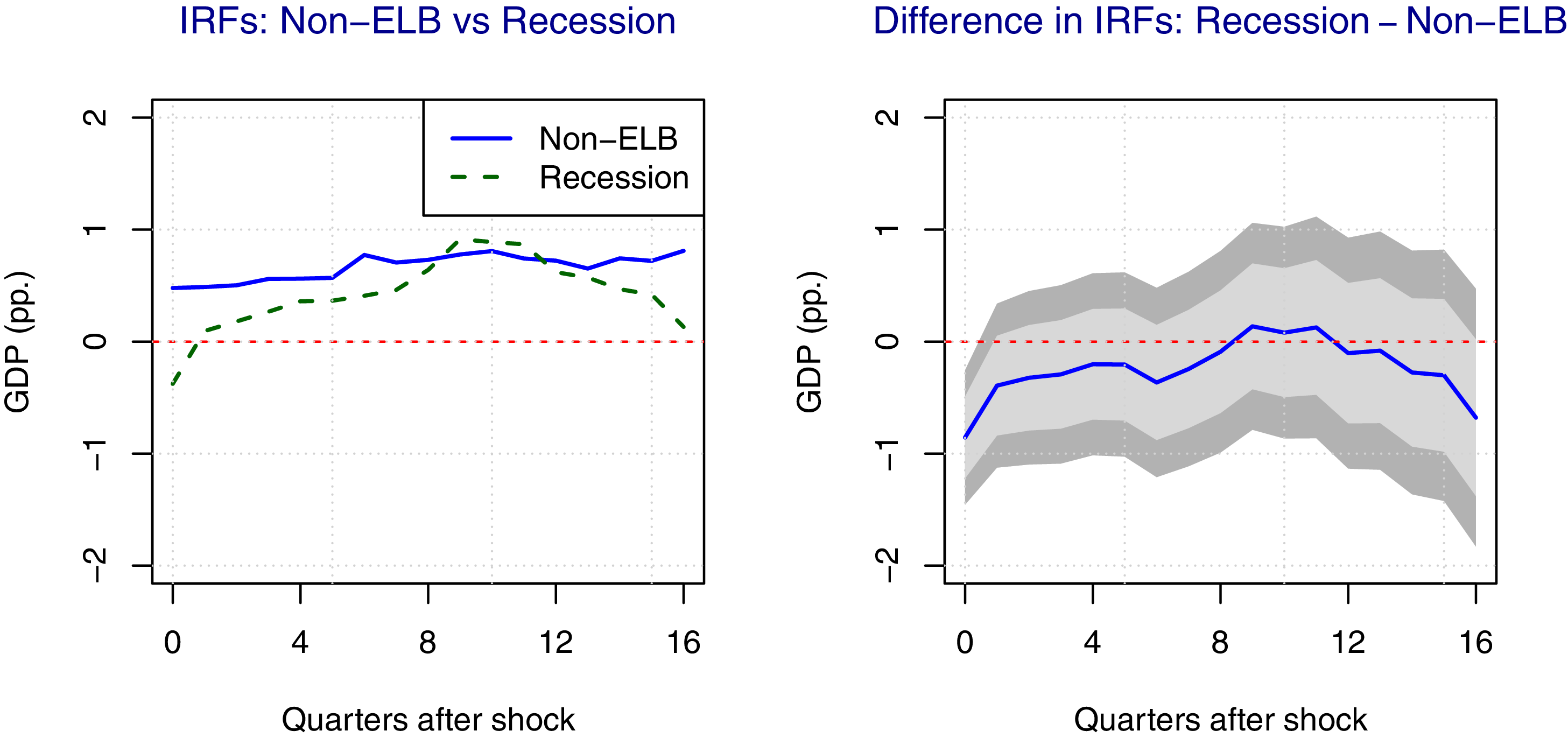
Estimating specification (3) allows me to simultaneously test if the transmission of productivity shocks is conditional on the state of the economy. I present the results in Figure 8, and show that barring the contemporaneous response, there is no evidence of output responding differently to productivity shocks in recessions in the long-run. The CD function is not statistically significant for any of the forecast horizons
 $k \geq 1$
. Thus, allowing me to conclude that productivity shocks have an expansionary effect on the economy, irrespective of the state of the business cycle. This is in stark contrast to the literature on fiscal policy (Auerbach and Gorodnichenko, Reference Auerbach and Gorodnichenko2012), monetary policy (Tenreyro and Thwaites, Reference Tenreyro and Thwaites2016), and oil prices (Hwang and Kim, Reference Hwang and Kim2024), which argue that the effects of shocks are different in recessions compared to expansions.
Cumulative response of GDP to productivity shocks in the normal monetary policy regime and recessions.
Note: The left panel represents the cumulative response of GDP to a one-standard deviation surprise productivity shock calculated using Eq. (3), and the right panel is the difference in response between the recession and non-ELB regimes, expressed as the cumulative difference functions. The light and dark gray shaded regions represent the 68% and 90% confidence intervals, respectively.

4.4 Empirical specification with inflation expectations
Utilizing the current inflation rate in the baseline specification implies that the nonlinear shock response of the ex-post real rate of interest changes the transmission of productivity shocks to the U.S. economy. To allow the possibility of the ex-ante real interest rate to change the transmission of these shocks, I estimate my baseline specification (3) by replacing the inflation rate with inflation expectations, as measured by the Survey of Professional Forecasters (SPF) and the Michigan Survey of Consumers. Based on the SPF, inflation expectations correspond to the median 4-quarter ahead annualized percent change in the price level. For the Michigan Consumer Survey, inflation expectations correspond to the expected median price change over the next 12 months. The data for this estimation exercise start in 1977 Q1 and end in 2022 Q1, which is dictated by the availability of Michigan Survey of Consumers’ inflation expectations data. An advantage of this subsample is that it places a greater weight on observations from the Great Moderation (
 $1984-2007$
) which was characterized by a significant reduction in the volatility of business cycle fluctuations. Thus, allowing me to rule out the possibility that the nonlinear response of the economy to productivity shocks is driven by the earlier time period,
 $1947 Q2-1977 Q4$
.
Figure 9 shows that while the cumulative response is not as strong as what is observed in Figure 2, productivity shocks continue to generate differential effects for the economy across each monetary policy regime. Productivity shocks are expansionary on impact. Results from the specification estimated with SPF inflation expectations indicates that the shock response of output peaks at 0.56 pp. after 11 quarters in the non-ELB regime. However, the same shock in the ELB generates a decline, with output decreasing by as much as 0.45 pp. after eight quarters. The difference in response between both regimes is also statistically significant. The results for output are identical if we use inflation expectations extracted from the Michigan Consumer Survey, as evident from the responses in the bottom row of Figure 9.
Cumulative response of GDP and inflation expectations to productivity shocks around the ELB.
Note: The top panel represents the cumulative response of GDP and inflation expectations (as measured by the Survey of Professional Forecasters) to a one-standard deviation surprise productivity shock, along with the difference in response between the ELB and non-ELB regimes, expressed as the cumulative difference functions. The bottom row corresponds to the specification estimated with the Survey of Consumers’ inflation expectations. The light and dark gray shaded regions represent the 68% and 90% confidence intervals, respectively.

Consistent with our results for inflation, I find that SPF inflation expectations decline following a positive productivity shock, though the response is stronger in the non-ELB regime compared to the ELB. The shock response of household inflation expectations is negative in the non-ELB, consistent with our SPF metric. However, there is little to no response in the ELB, which is puzzling. This suggests that while actual inflation and inflation expectations of professional forecasters exhibit a decline to a productivity shock in the ELB, this does not necessarily translate into lower expectations of inflation for households. These results emphasize that using inflation expectations and a shorter sample period does not alter the key results of the paper, that is, the effect of productivity shocks are conditional on the ELB.
4.5 Alternative empirical specification: LP-IV
The baseline model relies on the structural shock recovered from a SVAR and utilized in local projections, as is common practice in the literature (Ramey, Reference Ramey2016; Alloza, Reference Alloza2022; Adolfsen et al. Reference Adolfsen, Ferrari Minesso, Mork and Van Robays2024; Ciaffi et al. Reference Ciaffi, Deleidi and Di Domenico2024). However, it is worth noting that a SVAR model imposes the restriction that the relationship between productivity shocks and the economy is linear. This might be problematic because the recovered structural shock does not account for nonlinearities across each type of monetary policy regime. Consequently, applying these shocks directly in a state-dependent LP might lead to biased estimates for the cumulative difference functions.
To address this potential concern, and to maintain comparability with the findings of Garín et al. (Reference Garín, Lester and Sims2019), I conduct the inference in one step using the LP-IV framework following Ramey and Zubairy (Reference Ramey and Zubairy2018). This exercise is carried out by estimating Eq. (3) where
 $\varepsilon _{prod,t}$
is replaced with the growth of labor productivity,
 $\Delta prod_t$
, and instrumented with Fernald (Reference Fernald2014)’s series on the growth rate of utilization adjusted TFP. The calculation of the cumulative IRFs and difference functions follows the approach outlined in Section 2.2.2.
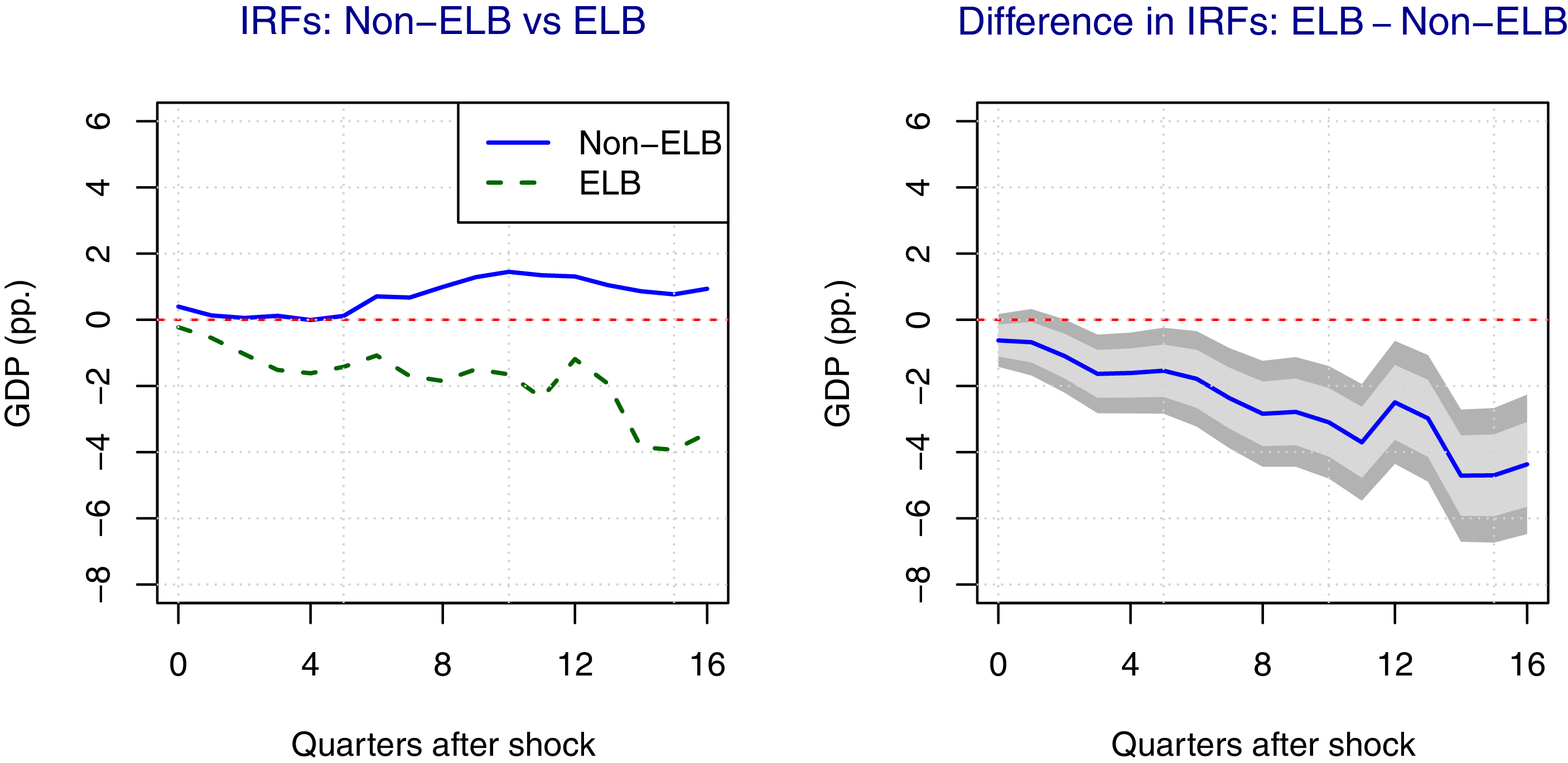
To maintain brevity, I only present the cumulative response of GDP to productivity shocks in Figure 10. The evidence of nonlinearity becomes quantitatively stronger when the IRFs are generated using LP-IV. Specifically, a one-standard deviation productivity shock in the non-ELB generates a cumulative increase in GDP across multiple forecast horizons, with the effect peaking at 1.51 pp. after 10 quarters compared to 0.82 pp. in Section 3.3. On the contrary, the drop in GDP is also more severe, with it declining by as much as 2.33 pp. after 10 quarters, almost four times stronger than the results from the baseline model. The cumulative difference functions are also statistically significant. Overall, the results from this section reinforce the point made earlier in the paper that the effects of productivity shocks are conditional on the monetary policy regime, and, as such the conflicting findings compared to Garín et al. (Reference Garín, Lester and Sims2019) are not driven by any potential methodological bias.
Cumulative response of GDP to productivity shocks estimated using LP-IV.
Note: The left panel represents the cumulative response of GDP to a one-standard deviation surprise productivity shock, and the right panel is the difference in response between the ELB and non-ELB regimes, expressed as the cumulative difference functions. The light and dark gray shaded regions represent the 68% and 90% confidence intervals, respectively.

Cumulative response of GDP to productivity shocks around the ELB defined as
 $i_t \leq 1.00\%$
.
Note: The left panel represents the cumulative response of GDP to a one-standard deviation surprise productivity shock, and the right panel is the difference in response between the ELB and non-ELB regimes, expressed as the cumulative difference functions. The light and dark gray shaded regions represent the 68% and 90% confidence intervals, respectively.

4.6 Alternative definitions for the Fed’s binding constraints
To incorporate the possibility of more general thresholds for constrained monetary policy, we rely on alternative definitions for the effective lower-bound (ELB) regime. Swanson and Williams (Reference Swanson and Williams2014) present evidence of the Federal Reserve’s binding constraint changing over time by showing how the response of Treasury yields to macroeconomic news in 2003-04 was very similar to the ELB period. This is despite the fact that the Federal Funds Rate was not constrained by a floor of zero in 2003-2004. Bernanke and Reinhart (Reference Bernanke and Reinhart2004) also reinforce this point by suggesting that 1% percent was considered a binding constraint in 2003. Consequently, I re-estimate specification (3) by defining ELB as
 $i_t\leq 1.00\%$
. Figure 11 shows that the effects of productivity shocks are different in each monetary policy regime, in line with my baseline results. Specifically, a positive productivity shock in the non-ELB (ELB) will be expansionary (contractionary). The CD functions in the right panel indicate that the difference in response is also statistically significant. This suggests the presence of thresholds more general than a FFR of 0.25% that could influence the state-dependent shock response of the economy.
4.7 Testing for size and sign nonlinearities
The current threshold model effectively captures regime dependence based on monetary policy constraints, but it would be informative to assess whether responses also differ by the sign or size of the productivity shock. To test for this, we follow Forni et al. (Reference Forni, Gambetti, Maffei-Faccioli and Sala2024), who offer a tractable framework for testing this directly in local projection settings. To account for potential nonlinearities surrounding the sign or size of the shock, and the respective regimes (ELB and recessions), I augment specification (3) with two additional terms. One of these, the absolute term of the shock
 $|\varepsilon _{prod,t}|$
, is meant to capture potential sign nonlinearities (Forni et al. Reference Forni, Franconi, Gambetti and Sala2025), and the cubic term,
 $(\varepsilon _{prod,t})^3$
, is intended to detect nonlinearities associated with the size of the shock (Tenreyro and Thwaites, Reference Tenreyro and Thwaites2016). The model takes the form:
 \begin{equation} \begin{aligned} \Delta {x}_{t+h} &=\alpha _{h}+\beta _{h}\varepsilon _{prod,t}+\sum _{l=1}^{n}X^{\prime}_{i,t-l}B_{h,l}+I_{t-1}^{elb}\times \left [\alpha _{h}^{elb}+\beta _{h}^{elb}\varepsilon _{prod,t}+\sum _{l=1}^{n}X^{\prime}_{i,t-l}B_{h,l}^{elb}\right ] \\ &\quad +\, I_{t-1}^{rec}\times \left [\alpha _{h}^{rec}+\beta _{h}^{rec}\varepsilon _{prod,t}+\sum _{l=1}^{n}X^{\prime}_{i,t-l}B_{h,l}^{rec}\right ]+\gamma ^{A}_h \times (\varepsilon _{prod,t})^3\\ &\quad +\, \gamma ^{B}_h\times |\varepsilon _{prod,_t}|+\sum _{l=1}^nC^{\prime}_{i,t-l}V_{h,l}+u_{t+h}. \end{aligned} \end{equation}
Where, the definition of the variables follows Section 2.2.2.
 $C^{\prime}_{i,t-l}$
includes lags of the absolute and cubic terms of the shock.
 $\beta ^{elb}_h$
,
 $\beta ^{rec}_h$
,
 $\gamma ^{A}_h$
, and
 $\gamma ^{B}_h$
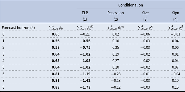
capture nonlinearities associated with the ELB, recession, size and sign of the shock, respectively. I presents results for the cumulative coefficients at each time horizon in Table 8. The estimates in the column for
 $\sum _{h=0}^{k}\beta _{h}$
indicate that productivity shocks generate a statistically significant expansion in output when the economy is operating away from the ELB (
 $I^{elb}_{t-1}=0$
) and not in a recession (
 $I^{rec}_{t-1}=0$
). Consistent with the findings in Sections 3.3 and 4.3, I find that productivity shocks have a contractionary effect when the economy is at the ELB (
 $\sum _{h=0}^k \beta _h^{elb}$
), whereas the state of the business cycle does not materially alter the propagation as none of the cumulative effects (
 $\sum _{h=0}^k \beta _h^{rec}$
) are statistically significant. Additionally, neither sign nor size asymmetries appear to matter, as the corresponding responses (columns 3 and 4) are not statistically significant. Taken together, these results suggest that the nonlinearities observed in the transmission of productivity shocks are driven primarily by the monetary policy regime rather than by any intrinsic features of the shocks themselves.
Marginal threshold effects of productivity shocks on output

Notes: This table reports the cumulative estimates of
 $\beta _{h}$
,
 $\beta _h^{elb}$
,
 $\beta _h^{rec}$
,
 $\gamma _{h}^{A}$
, and
 $\gamma _{h}^{B}$
estimated from equation (10) for each forecast horizon (
 $h$
). The estimated coefficients have been normalized to reflect the response to a one standard deviation productivity shock. Bold indicates that the point estimate is statistically significant, as 0 lies outside the 90% bootstrapped confidence bands.
5. Conclusion
The main motivation for this paper stems from the need to reconcile the state-dependent effects of productivity shocks at the ELB with a basic NK and medium scale macro model. My findings highlight that the response of the U.S. economy to productivity shocks is substantially different across each type of monetary policy regime. Specifically, these shocks tend to be expansionary (contractionary) when monetary policy is operating in the non-ELB (ELB) regime. I contribute to the literature by emphasizing the key role of the ELB in altering the transmission of productivity shocks, and also identifying the mechanism through which these shocks generate nonlinear responses. The interest-sensitive variables, such as business investment, private sector credit, and durable consumption, show considerable differences in their response to favorable productivity shocks, which then feeds into output. The results remain robust to alternative specifications and sample periods, thereby ruling out the possibility of the state-dependent effects driven by any potential methodological bias. It is worth noting that analyzing the economy’s response to productivity shocks within a linear framework overlooks potential nonlinearities that can arise due to the central bank’s binding constraints. This paper highlights the need to take into account the monetary policy regime when analyzing the effect of productivity shocks, which is line with the broader literature documenting the same for fiscal policy (Christiano et al. Reference Christiano, Eichenbaum and Rebelo2011), uncertainty (Plante et al. Reference Plante, Richter and Throckmorton2018), and oil price (Bodenstein et al. Reference Bodenstein, Guerrieri and Gust2013; Datta et al. Reference Datta, Johannsen, Kwon and Vigfusson2021; Sardar and Sharma, Reference Sardar and Sharma2022) shocks.
Acknowledgements
The author would like express their gratitude to the Associate Editor of Macroeconomic Dynamics, and two anonymous referees whose feedback and comments have been valuable in improving the quality of the paper.