


1. Introduction
This study is concerned with the eddy structures (ESs) and very-large-scale motions (VLSMs) in the (fully turbulent) intermediate field of turbulent round jets. The jet flow issuing from a contracting nozzle comprises three regions: the near field, the intermediate field and the far field. The near field, which appears only for jets issuing from a contracting nozzle, is defined by its potential core, and is usually within  $0 \leq x/d \leq 7$. The far field, located from approximately
 $x/d \geq 70$, is the self-similar region of the jet. The intermediate field is the streamwise region between the near and far fields and becomes fully turbulent from approximately
 $x/d \geq 10$ (Ball, Fellouah & Pollard Reference Ball, Fellouah and Pollard2012).
Our focus in the present study is on the jets that discharge from contracting nozzles. Before the introduction of coherent structures, turbulent flows were considered as random phenomena and were approached purely from a statistical point of view. The discovery of coherent structures in turbulent flows changed this view and facilitated notable advances in understanding the physics of turbulence as well as the control of turbulent shear flows (Hussain Reference Hussain1983). One of the chief applications of coherent structures is in the study of aerodynamic noise in the near field of turbulent jets (see e.g. Crow & Champagne Reference Crow and Champagne1971; Mankbadi & Liu Reference Mankbadi and Liu1984; Hussain Reference Hussain1986; Cavalieri et al. Reference Cavalieri, Rodríguez, Jordan, Colonius and Gervais2013; Fu et al. Reference Fu, Agarwal, Cavalieri, Jordan and Brès2017, among others). Interaction of the coherent structures is also crucial in mixing and entrainment (Winant & Browand Reference Winant and Browand1974; Philip & Marusic Reference Philip and Marusic2012) and the development of turbulent jets (Browand & Laufer Reference Browand and Laufer1975; Breda & Buxton Reference Breda and Buxton2018). In technological applications, coherent structures and their interactions could be artificially magnified or suppressed through excitation or interruption imposed on the flow with the purpose of enhancing heat transfer, mixing and entrainment as well as noise reduction (Zaman & Hussain Reference Zaman and Hussain1981; Sadeghi & Pollard Reference Sadeghi and Pollard2012). Hence, better understanding of the flow physics of coherent structures of various scales should lead to more efficient control of jets.
Coherent structures in axisymmetric jets that discharge from a contracting nozzle constitute a broad variety of scales and configurations that occur at different stages of the jet evolution (Ball et al. Reference Ball, Fellouah and Pollard2012), with vortex rings being the dominant structures in the transitional region in the near field of the turbulent round jet. Yule (Reference Yule1978) studied the transitional and fully turbulent region in the round jets. His experiments showed that Kelvin–Helmholtz instabilities produce a street of vortex-ring-like vorticity concentrations in the transitional region. As these vortex rings move downstream, they generally coalesce and break into three-dimensional large eddies. Yule emphasized that orderly, easily visualized, circumferentially coherent vortices in the transition regions of free shear flows are different from the less clearly visualized, but strong, large eddies in the fully turbulent region. Using laser-induced fluorescence measurements, Liepmann & Gharib (Reference Liepmann and Gharib1992) showed that, as the jet progresses into the turbulent region, azimuthal instabilities break the vortex rings by producing axial vortex pairs in what is referred to as the braid region. Distinct mushroom-like structures form around the jet potential core in this region and move outwards after their formation. Using stereoscopic particle image velocimetry (PIV) and resolvent analysis in the jet near field, Nogueira et al. (Reference Nogueira, Cavalieri, Jordan and Jaunet2019) showed that large-scale streaky structures and the lift-up mechanism, which are important phenomena in wall-bounded turbulence, are also relevant aspects of the jet dynamics in the near field.
Several studies suggest the presence of hairpin-like eddies as the main vortical structure in the fully turbulent region of the jet. Based on the correlation measurements of three velocity components in turbulent free shear flows, Townsend (Reference Townsend1976) suggested that the flow features are dominated by double-roller ESs that are inclined to the axial direction. Nickels & Perry (Reference Nickels and Perry1996) followed Townsend's proposal for the dominant ESs. They modelled the turbulent round jet using double-roller eddies with a characteristic velocity that is proportional to the centreline velocity of the jet, and a characteristic length that is proportional to the characteristic radius of the jet. Each of these eddies has a limited azimuthal extent and a number of them are randomly distributed in different azimuthal and axial positions with equal probability to form the flow. They used a single-size ES to model the jet flow and observed fairly good agreement between the Reynolds stresses and energy spectra calculated from this model compared to those from experiments.
The single-size ES model in the turbulent round jet is in contrast to hierarchies of ESs required to model turbulent wall-bounded flows (Nickels & Marusic Reference Nickels and Marusic2001). Using two-point correlations of temperature and velocity fluctuations obtained from direct numerical simulation (DNS) of a round jet at a jet Reynolds number  $Re_d= \langle U_j \rangle d/\nu = 1200$, Suto et al. (Reference Suto, Matsubara, Kobayashi, Watanabe and Matsudaira2004) showed that both temperature and velocity can be used as an indicator of an eddy. Here
 $\langle U_j \rangle$ is the jet mean velocity,
 $d$ is the nozzle diameter and
 $\nu$ is the fluid kinematic viscosity. They proposed a conceptual model of a hairpin-like eddy and validated it by two-point correlations and probability density function analysis for the eddy alignment. They found that the eddies stand with their legs inclined downstream at an inclination angle of
 $45^\circ$, suggesting that a hairpin-like eddy is one of the universal structures in turbulent shear flows. The inclined legs of these eddies are consistent with the mushroom-like structures reported by Liepmann & Gharib (Reference Liepmann and Gharib1992) in the braid region.
Matsuda & Sakakibara (Reference Matsuda and Sakakibara2005) used time-resolved stereo PIV measurements to study the turbulent region of the jet up to  $Re_d=5000$. They used isosurfaces of the swirling strength and revealed the existence of a group of hairpin-like ESs around the rim of the shear layer of the jet. Hairpin-like ESs have also been reported in DNS of the turbulent region of round jets (e.g. Wang et al. Reference Wang, He, Lv, Zhou, Fan and Cen2010; Tyliszczak & Geurts Reference Tyliszczak and Geurts2014; Anghan et al. Reference Anghan, Dave, Saincher and Banerjee2019). Recently, Samie, Lavoie & Pollard (Reference Samie, Lavoie and Pollard2020) applied a spectral analysis to datasets of two-point measurements in the turbulent region of round jets with radial separations between the sensors, and showed that hierarchical ESs are embedded in the jet. They also showed that the coherent ESs are self-similar in the jet shear layer and estimated a stochastic axial–radial aspect ratio of
 for them.
Contrary to the vortex rings in the near field, and the ESs in the transitional and fully turbulent regions, there is hardly any consensus on the configuration of the dominant VLSMs in the fully turbulent region of round jets. This is probably due to the superposition of structures of various sizes, which complicates inference of the dominant very-large-scale coherent structures. The main structures reported as the predominant VLSMs in the fully turbulent region of round jets are rings, single helices and double helices. Using laser-induced fluorescence measurements and observational reasoning, Dimotakis, Miake-Lye & Papantoniou (Reference Dimotakis, Miake-Lye and Papantoniou1983) concluded that the far field of the turbulent round jet is predominantly organized in the form of very-large-scale axisymmetric or helical structures, or in a transitional state between these two configurations. Based on modal analysis Fiedler (Reference Fiedler1988) stated that rings, single helices and double helices are the first three modes in the turbulent round jet, which are approximately equally distributed.
Tso & Hussain (Reference Tso and Hussain1989) used a rake of radially organized cross-wires to deduce very-large-scale coherent structures in the far field of a turbulent round jet. Their results showed that VLSMs with axisymmetric, helical and double helical configurations are present in the flow, among which the helical structures are far more dominant than the others. Yoda, Hesselink & Mungal (Reference Yoda, Hesselink and Mungal1994) measured the concentration of the turbulent round jet and, based on these results, proposed that the structure of the far field of the jet consists not of a single expanding helical structure, but of a pair of expanding counter-rotating helical vortex filaments. Recently, Mullyadzhanov et al. (Reference Mullyadzhanov, Sandberg, Abdurakipov, George and Hanjalić2018) analysed results from DNS of a turbulent round jet issuing from a fully developed pipe at  $Re=5940$ based on the bulk velocity in the pipe and its diameter. Their results showed that a propagating helical wave represents the optimal eigenfunction for the flow, and the first two mirror-symmetric modes containing approximately
 $5\,\%$ of the total turbulent kinetic energy capture all significant large-scale features.
Some of the extensively used techniques to extract coherent structures in turbulent flows are proper orthogonal decomposition (e.g. Glauser, Leib & George Reference Glauser, Leib and George1987; Delville et al. Reference Delville, Ukeiley, Cordier, Bonnet and Glauser1999; Jung, Gamard & George Reference Jung, Gamard and George2004), spectral proper orthogonal decomposition (e.g. Schmidt et al. Reference Schmidt, Towne, Rigas, Colonius and Brès2018; Towne, Schmidt & Colonius Reference Towne, Schmidt and Colonius2018) and dynamic mode decomposition (e.g. Schmid Reference Schmid2010; Semeraro, Bellani & Lundell Reference Semeraro, Bellani and Lundell2012). In the present study, the linear coherence spectrum (LCS) (Bendat & Piersol Reference Bendat and Piersol2011), which is a normalized scale-by-scale correlation between two signals, together with two-point correlation are used to educe coherent features of different sizes in turbulent round jets. The LCS has been used previously to assess coherent structures in wall-bounded turbulent flows (e.g. Bailey et al. Reference Bailey, Hultmark, Smits and Schultz2008; Baars, Hutchins & Marusic Reference Baars, Hutchins and Marusic2016, Reference Baars, Hutchins and Marusic2017; Baidya et al. Reference Baidya2019).
Despite numerous studies conducted on the coherent structures in the fully turbulent region of round jets over the past five decades or so, it is not clearly known whether the ESs and VLSMs are completely independent entities or somehow connected. It is also unclear why an axial–radial aspect ratio of  was found for the ESs by Samie et al. (Reference Samie, Lavoie and Pollard2020), while the axial and radial spans of a typical hairpin-like eddy are of
 ${O}(1)$ according to the eddy visualizations. Furthermore, doubts still exist on the configuration of VLSMs in turbulent round jets. To address these issues, two-point simultaneous velocity measurements are conducted with separating radial and azimuthal distances between the sensors in the fully turbulent region of round jets across the Reynolds-number range
 $Re_d=10\,000\text {--}50\,000$. Spectral analysis is applied to the data to assess the coherent structures in both radial and azimuthal directions. Moreover, instantaneous velocity fluctuations from a DNS of a turbulent jet at
 $Re_d=7920$ from Shin, Sandberg & Richardson (Reference Shin, Sandberg and Richardson2017) are used to complement our analysis.
The rest of the paper is organized as follows. Experimental details are presented in § 2. Experimental two-point correlations are discussed in § 3.1. A scale-dependent correlation is introduced and applied to the experimental axial velocity signals in § 3.2. Based on this scale-dependent correlation, a filter is introduced in § 3.3, which is used to isolates the VLSMs, thereby shedding light on the configuration of the VLSMs. This is achieved by inspecting the filtered correlation maps of axial velocities. Using the isolated VLSMs, it is hypothesized that helical structures are the dominant VLSMs in turbulent round jets. VLSMs and ESs from an existing DNS study are discussed in § 4, where the prevalence of helical structures is further supported. In § 5, two synthetic flow fields are generated to simulate the configuration of the VLSMs and a simplified model is proposed for the arrangement of the ESs and VLSMs based on the observations from experiment, DNS and synthetic flow fields. Finally, concluding remarks are presented in § 6.
2. Experimental details
Measurements were conducted in the intermediate region of a round jet using the facility described in Fellouah, Ball & Pollard (Reference Fellouah, Ball and Pollard2009) and Samie et al. (Reference Samie, Lavoie and Pollard2020). The jet air flow is produced by a fan mounted on anti-vibration pads. The fan exhaust is connected to the jet settling chamber through a flexible hose. The settling chamber consists of a filter, a flow-straightening section and three screens with different porosities, which break down any large-scale structures, thereby ensuring a clean air flow at the jet exit. The air exhausts through a round duct to the inlet of a smoothly contracting axisymmetric nozzle with fifth-order polynomial wall contour. The exit diameter of the nozzle is  $d=73.6\ \textrm {mm}$, producing a top-hat distribution velocity profile. More details about the jet facility can be found in Fellouah et al. (Reference Fellouah, Ball and Pollard2009).
Two single hot wires were used to simultaneously acquire the axial fluctuating velocity of the turbulent jet at various axial and radial distances from the jet exit and jet centreline, respectively. The sensing elements of the wires were  $5\ \mathrm {\mu }\textrm {m}$ in diameter and
 $1000\ \mathrm {\mu }\textrm {m}$ in length. This results in a sensor length-to-diameter ratio of 200, which ensures minimal end conduction effects in the hot wires (Ligrani & Bradshaw Reference Ligrani and Bradshaw1987; Samie, Hutchins & Marusic Reference Samie, Hutchins and Marusic2018). The wire elements are made of tungsten and were manufactured by Auspex Corporation. The hot wires were calibrated against a Pitot-static tube in the potential core of the jet at
 $x/d \approx 0$, where the mean velocity profile is flat and the axial velocity fluctuations are less than 1 % of the mean jet velocity, before and after each experiment. This resulted in two to five hour time intervals between the pre- and post-calibrations depending on the experiment duration. The experimental data were used only if the difference between the pre- and post-calibration curves was below 1 %. The hot wires were powered by a Dantec Streamline constant-temperature hot-wire anemometer with an overheat ratio of 1.8.
The laboratory temperature was recorded at two locations near and far from the jet exit before and after each experimental run, and its variation was always within  ${\pm }2\,^{\circ }\textrm {C}$. Third-order polynomial curves were fitted to the calibration data. The hot-wire signals were sampled using a 16-analogue-input multifunction data acquisition (DAQ) card PCI-6052E (
 $333\ \textrm {kS}\ \textrm {s}^{-1}$, 16 bit), and a National Instruments SCXI signal conditioning at a sampling frequency
 $f_s = 7\ \textrm {kHz}$ and low-pass filtered using an analogue filter at
 $f_{lp} = 3\ \textrm {kHz}$ to avoid aliasing. This is well beyond the maximum frequency content of the axial energy spectra anywhere in the present flow. The total sampling time at each measurement location is given by
 $T$ and is normalized to give the eddy turnovers
 $TU_{ref}/y_{0.5}$, where
 $U_{ref}$ is the velocity at the reference sensor location and
 $y_{0.5}$ is the jet half-width and is determined as the radial location at which the mean axial velocity is equal to half of the mean axial velocity at the centreline. In order to obtain converged spectra and two-point correlations, this number should be large to capture several hundreds of the largest structures past the sensor. In the present study
 $TU_{ref}/y_{0.5}=3000\text {--}9700$ for all the measurements. The smallest eddy turnover values are associated with the lowest-Reynolds-number measurements. A convergence test was conducted for the spectra with the smallest eddy turnover values, and results of the test ensured convergence of the spectra for all the measurements.
Simultaneous axial velocity signals were acquired using two different hot-wire arrangements, as shown schematically in figure 1. In the radial arrangement displayed schematically in figure 1(a), two hot-wire probes were mounted on a 1 m long vertical aerodynamic sting using a probe holder, thereby allowing one hot wire to be fixed at the reference radial distance from the jet centreline ( $y_{ref}$), while a second hot wire was traversed incrementally to obtain various radial separations (
 $\Delta y$) between the two hot wires. In the azimuthal arrangement, as shown in figure 1(b), where the jet cross-stream plane at the hot-wire locations is displayed schematically, the traversing system was designed such that one probe could be positioned at an adjustable radial distance from the centreline, while the second probe at the same radial distance from the centreline could be azimuthally traversed to obtain various azimuthal separations between the probes (
 $\Delta s=y \Delta \theta$). The shaft around which the traverse arms were rotated was nominally fixed on the jet centreline. Measurements were made in the range
 $x/d=15\text {--}25$, in both radial and azimuthal arrangements, and at three Reynolds numbers,
 $Re_d=10\,000$,
 $20\,000$ and
 $50\,000$. The flow was fully turbulent at all measurement locations and Reynolds numbers.
Arrangement of the hot-wire probes for (a) the radial measurements and (b) the azimuthal measurements. TNTI is the turbulent/non-turbulent interface.

3. Experimental results
3.1. Two-point correlation
The cross-correlation function between two velocity time series  $u(x, y_{ref};t)$ and
 $u(x, y_{ref} + \Delta y, \Delta s; t)$ is defined as
 \begin{equation} R_{uu}(x,y_{ref},\Delta y, \Delta s;\tau) = \dfrac{\langle u(x,y_{ref};t)\,u(x,y_{ref}+\Delta y,\Delta s; t+\tau)\rangle} {\sigma_u(x,y_{ref})\,\sigma_u(x,y_{ref}+ \Delta y, \Delta s)}, \end{equation}
where the angle brackets indicates a time averaging,  $x$ is the axial location of the sensors,
 $y_{ref}$ is the radial location of the reference sensor,
 $\Delta y$ and
 $\Delta s$ are the radial and azimuthal distances between the traversing and the reference sensors, respectively, and
 $\sigma _u$ denotes the root-mean-square value of velocity fluctuations
 $u$ (
 $\equiv U-\langle U \rangle$).
First,  $R_{uu}$ is considered for the radial measurements where
 $\Delta s=0$ while
 $\Delta y$ is varied. Reynolds-number comparison of the radial correlation contours at normalized radial reference distances from the centreline
 $y_{ref}/y_{0.5} \approx 0$, 0.3 and 0.6 (where
 $y_{0.5}$ is the jet half width) and an axial distance from the jet nozzle exit
 $x=15d$ is shown in figure 2. The correlation contours are presented as a function of
 $\Delta y/y_{0.5}$ and
 $\tau \langle U \rangle /y_{0.5}$, where
 $\langle U \rangle$ is the local mean velocity. Let us assume that (for the purpose of comparison only) the integral time scale is identified by the correlation level
 $R_{uu}=0.2$. No perceptible Reynolds-number dependence for the integral time scale is observed based on this definition for
 $Re_d=10\,000\text {--}50\,000$. Note that the above-mentioned findings can be made on the integral length scale by invoking Taylor's frozen-eddy hypothesis to convert time to length scales. Interestingly, for
 $y_{ref}/y_{0.5}=0$, there is a negative correlation region for
 $\Delta y/y_{0.5}>0.6$ around
 $\tau \langle U \rangle /y_{0.5}=0$. Note that, although in figure 2(a) the negative region is shown only for
 $Re_d=10\,000$, there are similar negative correlation regions for
 $Re_d=20\,000$ and
 $50\,000$ for
 $y_{ref}/y_{0.5}>0.6$. While the correlation contours are virtually symmetric with respect to
 $\tau \langle U \rangle /y_{0.5}=0$ at
 $y_{ref}/y_{0.5} \approx 0$, the coherent structures appear to be forward-inclined (inclined opposite to the flow direction) at
 $y_{ref}/y_{0.5} \approx 0.3$ and 0.6, and the inclination angle changes with
 $y_{ref}$. The inclination angle of coherent structures is inferred from the correlation contours via (3.2) in a process illustrated in figure 3.
Effect of Reynolds number on the radial correlation maps (as functions of  $\Delta y/y_{0.5}$ and
 $\tau \langle U \rangle /y_{0.5}$) at (a)
 $y_{ref}/y_{0.5} \approx 0$, (b)
 $y_{ref}/y_{0.5} \approx 0.3$ and (c)
 $y_{ref}/y_{0.5} \approx 0.6$. For all the measurements in this figure,
 $x/d=15$ and the positive contour levels are
 $R_{uu}=$ 0.2, 0.4 and 0.6. In panel (a), a contour level of
 $R_{uu}=-0.1$ is shown for
 $Re_d=10\,000$ only; this contour level is not displayed for other Reynolds numbers for clarity.

(a) Correlation curves at various  $\Delta y$ spacings and (b) the corresponding correlation map at
 $x/d=15$,
 $Re_d=50\,000$ and
 $y_{ref}/y_{0.5} \approx 0.6$. Open circles depict the correlation peaks and are shown for every other point for clarity. The green line represents the average inclination angle,
 $\theta _m$. (c) Averaged angle of the coherent structures as a function of
 $y_{ref}/y_{0.5}$ for different Reynolds numbers and axial locations.

The inclination angle of coherent structures with respect to the axial direction can be quantified using the two-point correlation. Following Marusic & Heuer (Reference Marusic and Heuer2007), the inclination angle  $\theta$ is defined as
 \begin{equation} \theta(x, y_{ref},\Delta y) \equiv \tan^{{-}1} \left( \dfrac{\Delta y}{\Delta x^*} \right), \end{equation}
where  $\Delta y$ is the radial distance and
 $\Delta x^*$ is the spatial delay in the axial direction corresponding to a peak in the correlation
 $R_{uu}$. Time is converted to space using Taylor's frozen-eddy hypothesis. That is,
 $\Delta x^*=\tau _{max} \langle U \rangle$, where
 $\langle U \rangle$ is the local axial mean velocity and
 $\tau _{max}$ is the time shift corresponding to the peak in the correlation. Taylor's frozen-eddy hypothesis can be used when a good approximation of the convection velocity is available. Matsuda & Sakakibara (Reference Matsuda and Sakakibara2005) showed for turbulent round jets that the local mean velocity and convection velocity are virtually equal for radial distances up to
 $y/y_{0.5}=1$ in the turbulent region of round jets.
Figure 3(a) presents the correlation curves,  $R_{uu}$, for a number of
 $\Delta y$ separations for
 $x/d=15$,
 $y_{ref}/y_{0.5} \approx 0.6$ and a jet Reynolds number of
 $Re_d=50\,000$. Peaks of
 $R_{uu}$ are marked by open circles. It can be seen that the time shift corresponding to the peak of
 $R_{uu}$ grows with increasing
 $\Delta y$. The corresponding correlation contour map is presented in figure 3(b), where
 $R_{uu}$ is plotted as a function of
 $\Delta y/y_{0.5}$ and
 $\tau \langle U \rangle /y_{0.5}$. In figure 3(a,b), the open circles denote the peaks in the correlation at each
 $\Delta y/y_{0.5}$ and the inclination angle
 $\theta$ is displayed for a sample point (
 $\Delta y/y_{0.5}=0.44$). Note that in figure 3(a,b), only every other measurement point is shown for clarity. The green line represents the average inclination angle
 $\theta _m$, which is calculated by averaging over all inclination angles corresponding to the correlation peaks that satisfy
 $R_{uu} \geq 0.2$. Correlation peaks smaller than 0.2 are excluded from the averaging to avoid inaccuracies due to low signal-to-noise ratios. The average inclination angles are calculated in this way for various
 $x/d$ locations, Reynolds numbers and
 $y_{ref}/y_{0.5}$ values and are given in figure 3(c). In general, the average inclination angle decreases with an increase in
 $y_{ref}/y_{0.5}$.
Azimuthal correlations combined with radial correlations can provide insight into the three-dimensional features of the coherent structures. In relation (3.1), if the radial separation between the sensors is zero,  $\Delta y=0$, and the azimuthal distance
 $\Delta s$ is varied, azimuthal correlations will be obtained. The velocity data acquired using the hot-wire arrangement in figure 1(b) are used to determine the azimuthal correlations. The azimuthal correlation maps are compared for
 $Re_d=20\,000$ and
 $Re_d=50\,000$ at
 $y/y_{0.5} \approx 0.3$ and 0.5 in figure 4. The length scales, estimated by the correlation contour levels, display no evident sign of Reynolds-number dependence. A clear characteristic of the correlation contour maps in an axial–azimuthal plane is a negative correlation lobe alongside the positive correlation lobe. This is observed in all the cases displayed in figure 4. Similar results have been reported in turbulent jets (Ukeiley et al. Reference Ukeiley, Tinney, Mann and Glauser2007), pipes and channels (Monty et al. Reference Monty, Stewart, Williams and Chong2007; Baltzer, Adrian & Wu Reference Baltzer, Adrian and Wu2013; Lee, Sung & Adrian Reference Lee, Sung and Adrian2019) and boundary layers (Hutchins & Marusic Reference Hutchins and Marusic2007; Sillero, Jiménez & Moser Reference Sillero, Jiménez and Moser2014), and have been linked to coherent structures. In fact, Townsend (Reference Townsend1976) used these similarities in the correlations to propose similar ESs as the dominant features of all turbulent shear flows.
Effect of Reynolds number on the azimuthal correlation maps (as functions of  $\Delta s/y_{0.5}$ and
 $\tau \langle U \rangle /y_{0.5}$) at (a)
 $y/y_{0.5} \approx 0.3$ and (b)
 $y/y_{0.5} \approx 0.5$. For the results presented here,
 $x/d=15$. Solid lines represent correlation levels of
 $R_{uu}= 0.1$, 0.3 and 0.6, and the dashed line corresponds to a correlation level of
 $R_{uu}= -0.05$.

3.2. Scale-dependent correlation
While a two-point correlation gives an estimate of the coherent structures averaged over all length scales, a scale-by-scale correlation can be insightful for unravelling contributions from each scale of motion to the correlation. A scale-by-scale correlation between two velocity signals can be obtained by the LCS. The LCS (Bendat & Piersol Reference Bendat and Piersol2011) is given by
 \begin{align} \gamma_L^2(x,y_{ref}, \Delta y,\Delta s;f) &= \frac{\vert \langle \tilde{U}(x,y_{ref};f)\, \tilde{U}^\ast (x,y_{ref}+\Delta y,\Delta s;f)\rangle \vert ^2} {\langle \vert\tilde{U}(x,y_{ref};f) \vert ^2 \rangle \langle\vert\tilde{U}(x,y_{ref}+\Delta y, \Delta s;f)\vert^2\rangle} \nonumber\\ &=\frac{\vert \phi_{u_r u}^\prime(x,y_{ref}, \Delta y,\Delta s;f) \vert^2} {\phi_{u_r u_r}(x,y_{ref};f)\,\phi_{u u}(x,y_{ref}+\Delta y, \Delta s;f)}, \end{align}
where  $\tilde {U}$ is the Fourier transform of
 $u$ in time or space based on the dataset, which leads to the calculation of
 $\gamma _L^2$ in the frequency (
 $f$) or wavelength (
 $\lambda _x$) domain, respectively. When
 $\gamma _L^2$ is calculated in the frequency domain, it will be converted to the wavelength domain by invoking Taylor's frozen-eddy hypothesis,
 $\lambda _x=\langle U \rangle /f$, where
 $\langle U \rangle$ is the local axial mean velocity used as the convection velocity. Angle brackets,
 $\langle {~}\rangle$, indicate ensemble averaging, vertical bars,
 $\vert {~}\vert$, denote the modulus and an asterisk,
 $\ast$, indicates the complex conjugate. Therefore, the LCS is the ratio of the cross-spectrum magnitude squared and the product of the power spectral density of the two velocity signals. Following this definition,
 $\gamma _L^2$ is bounded by 0 (no coherence) and 1 (complete coherence).
The radial LCS can be obtained by setting  $\Delta s=0$ in (3.3). Figure 5(a) presents two sample velocity signals acquired simultaneously in the turbulent jet flow at
 $Re_d=50\,000$ and
 $x/d=15$. The LCS is computed for these signals and is shown as a function of wavelength (
 $\lambda _x$) in figure 5(b). It can be seen that
 $\gamma _L^2 \approx 0$ for
 $\lambda _x<0.1$ m and increases with
 $\lambda _x$ in the wavelength range
 $\lambda _x=0.1\text {--}0.7\ \textrm {m}$, beyond which it plateaus and becomes approximately wavelength-independent.
(a) Sample simultaneously acquired velocity signals  $u(y_{ref};t)$ and
 $u(y_{ref}+\Delta y;t)$ in the turbulent jet and (b) associated LCS against wavelength
 $\lambda _x$.

A  $\gamma _L^2$ spectrogram is generated when
 $\gamma _L^2$ is plotted against
 $\lambda _x$ and
 $\Delta y$. A Reynolds-number comparison of the radial
 $\gamma _L^2$ spectra is presented in figure 6 for three
 $y_{ref}/y_{0.5}$ values. A common feature of the LCS is that, at a constant
 $\Delta y$ (i.e. a horizontal line on the spectrogram),
 $\gamma _L^2$ reaches its highest value at relatively large wavelengths (
 $\lambda _x/y_{0.5}>4$). Moreover, by increasing
 $\Delta y$, non-zero coherence becomes increasingly confined to larger wavelengths. The reason for this observation is that, by increasing
 $\Delta y$, smaller eddies are no longer present as common contributors to the simultaneously acquired signals. It can be seen in figure 6 that the LCS contour lines are aligned with
 $\lambda _x \propto \Delta y^p$ for
 $\lambda _x/y_{0.5} \approx 0.2\text {--}4$ and then become approximately wavelength-independent beyond
 $\lambda _x/y_{0.5} \approx 4$ (marked by the vertical dotted line) in all cases. Furthermore, no noticeable Reynolds-number dependence is observed in the coherence spectrograms.
Reynolds-number comparison of radial coherence spectra at different  $y_{ref}$ locations, at
 $x/d=15$: (a)
 $y_{ref}/y_{0.5} \approx 0$, (b)
 $y_{ref}/y_{0.5} \approx 0.3$ and (c)
 $y_{ref}/y_{0.5} \approx 0.6$. The vertical dotted lines correspond to
 $\lambda _x/y_{0.5}=4$.

Using the LCS, Samie et al. (Reference Samie, Lavoie and Pollard2020) showed that hierarchical ESs corresponding to the wavelength range  $\lambda _x/y_{0.5} \approx 0.2\text {--}4$ are ingrained in turbulent round jets and are self-similar in the shear layer with
 $p=1$. The power
 $p=0.72$ at the centreline, and increases to
 $p=0.9$ at
 $y_{ref}/y_{0.5} \approx 0.3$ and finally to
 $p=1$ at
 $y_{ref}/y_{0.5} \approx 0.6$. In the shear layer (
 $y_{ref}/y_{0.5} \approx$ 0.6),
 $\lambda _x \approx 4.7 \Delta y$. Following Samie et al. (Reference Samie, Lavoie and Pollard2020) and Baars et al. (Reference Baars, Hutchins and Marusic2017), the constant of proportionality between
 $\Delta y$ and
 $\lambda _x$ is defined as the axial–radial aspect ratio of the self-similar ESs,
 . The axial–radial aspect ratio
 is obtained by fitting
 to the
 $\gamma _L^2$ surface in the wavelength range
 $\lambda _x/y_{0.5}=0.2\text {--}4$. For a detailed analysis of the LCS and its features in turbulent round jets, see Samie et al. (Reference Samie, Lavoie and Pollard2020).
The azimuthal LCS is obtained if  $\Delta y=0$ and
 $\Delta s$ is varied. The azimuthal LCSs are compared for
 $Re_d=20\,000$ and
 $50\,000$ at
 $y/y_{0.5} \approx 0.3$ and 0.5 in figure 7. A good agreement is observed between the two Reynolds numbers at both normalized radial locations. The azimuthal LCS can be divided into two main wavelength domains. The first main domain itself (
 $\lambda _x/y_{0.5} \approx 0.2\text {--}4$) is divided into two subdomains: in the range
 $\lambda _x/y_{0.5} \approx 0.2\text {--}0.8$ the contour lines are aligned with
 $\lambda _x \propto \Delta s$ (blue solid line) and in the range
 $\lambda _x/y_{0.5} \approx 0.8\text {--}4$ they are aligned with
 $\lambda _x \propto \Delta s^{0.7}$ (red dashed line). The second main domain is associated with
 $\lambda _x/y_{0.5}>4$, in which the contour lines are approximately wavelength-independent. Therefore, the ESs associated with the first subdomain (
 $\lambda _x/y_{0.5} \approx 0.2\text {--}0.8$ and
 $\Delta s/y_{0.5} \approx 0.05\text {--}0.16$) are self-similar and an axial–azimuthal aspect ratio (
 ) can be defined for them. It is interesting to note that
 . Non-self-similarity of the larger eddies (
 $\lambda _x/y_{0.5} \approx 0.8\text {--}4$ and
 $\Delta s/y_{0.5}>0.16$) is most likely due to the spatial constraints. Specifically, since the size of these ESs is comparable to the perimeter of the round jet, they have to follow the circular curvature of the jet, whereas the shape of the smaller ESs is independent of the jet curvature.
Azimuthal coherence spectrograms at  $Re_d=20\,000$ and
 $50\,000$ for
 $x/d=15$: (a)
 $y/y_{0.5} \approx 0.3$ and (b)
 $y/y_{0.5} \approx 0.5$. Here,
 $y$ is the radial distance of both sensors from the centreline.

The azimuthal  $\gamma _L^2$ spectra are compared for
 $x/d=15$ and 25 in figure 8 at
 $y/y_{0.5} \approx 0.5$ and 0.7. It is evident that the axial location has minimal effect on the azimuthal LCS for
 $x/d=15\text {--}25$; two main wavelength domains and two subdomains are again observed in the LCS, similar to figure 7.
Azimuthal coherence spectrograms at  $x/d=15$ and 25 for
 $Re_d=50\,000$: (a)
 $y/y_{0.5} \approx 0.5$ and (b)
 $y/y_{0.5} \approx 0.7$. Here,
 $y$ is the radial distance of both sensors from the centreline.

The physical dimensions of ESs ( $\mathcal {L} \times \mathcal {H} \times \mathcal {W}$) can be characterized based on the axial–radial and axial–azimuthal spectral aspect ratios acquired from
 $\gamma _L^2$ spectra. Here,
 $\mathcal {L}$,
 $\mathcal {H}$ and
 $\mathcal {W}$ are the length, height and width of an ES, respectively. Baidya et al. (Reference Baidya2019) illustrated that a spectral axial–azimuthal aspect ratio (
 ) inferred from the
 $\gamma _L^2$ contours is associated with a mean physical axial–azimuthal aspect ratio of
 . Therefore,
 in the pipe flow leads to
 $\mathcal {L}/\mathcal {W}=7$. Similarly, we can show that
 in the turbulent round jet imply
 $\mathcal {L}/\mathcal {H} \approx \mathcal {L}/\mathcal {W} \approx 1.2$. Therefore, ESs in turbulent round jets have a mean physical aspect ratio of
 $1.2:1:1$ in the axial, radial and azimuthal directions, respectively. Comparison of the physical aspect ratio for a turbulent jet with that for wall-bounded turbulent flows, which is
 $7:1:1$ (Baidya et al. Reference Baidya2019), shows that the ESs are considerably shorter in turbulent jets. The physical aspect ratio of
 $7:1:1$ for pipe flow is consistent with the notion of eddy packets in wall-bounded flows (e.g. Head & Bandyopadhyay Reference Head and Bandyopadhyay1981; Zhou et al. Reference Zhou, Adrian, Balachandar and Kendall1999; Adrian, Meinhart & Tomkins Reference Adrian, Meinhart and Tomkins2000; Guala, Hommema & Adrian Reference Guala, Hommema and Adrian2006; Adrian Reference Adrian2007; Lee et al. Reference Lee, Sung and Adrian2019). On the other hand, the physical aspect ratio of
 $1.2:1:1$ in jet flows suggests that ESs do not form hierarchical packets of eddies in the turbulent round jet.
While the LCS represents the coherence scale of the Fourier modes, the phase,  $\varPhi$, contains the shift of each Fourier mode between
 $u_{ref}$ and
 $u$, and therefore can be used as a scale-by-scale indicator of the shift between two velocity signals. Hence, it can be used to determine the scale-by-scale angle of structures with respect to a reference point. To this end, the cross-spectrum, which is related to the cross-correlation using
 $\phi _{u u}^\prime =\mathcal {F}\{ R_{uu}\}$ and is complex-valued, is used to define the phase as
 \begin{equation} \varPhi(x,y_{ref}, \Delta y;f) = \tan^{{-}1} \left\{\frac{\mathrm{Im}(\phi_{u u}^\prime)}{\mathrm{Re}(\phi_{u u}^\prime)} \right\}, \end{equation}
where  $\mathrm {Im}$ and
 $\mathrm {Re}$ indicate the imaginary and real components of
 $\phi _{uu}^\prime$, respectively, and
 $\varPhi$ is in radians. Since
 $\varPhi$ is only determined for the synchronized data with radial separation between the sensors,
 $\Delta s$ is not included in (3.4). Following Baars et al. (Reference Baars, Hutchins and Marusic2016), a scale-dependent time shift can be defined as
 $\tau _s(x,y_{ref}, \Delta y;f) \equiv \varPhi (x,y_{ref}, \Delta y;f) /(2 {\rm \pi}f)$ and subsequently a scale-dependent axial shift is obtained by invoking Taylor's frozen-eddy hypothesis as
 $\Delta x_s^*=\tau _s \langle U \rangle$. A scale-dependent physical inclination angle is then computed following
 \begin{equation} \theta_s(x,y_{ref}, \Delta y;f)=\tan^{{-}1} \left( \dfrac{\Delta y}{\Delta x_s^*} \right). \end{equation}
Contour plots of  $\theta _s(\Delta y; \lambda _x)$ overlaid on the
 $\gamma _L^2$ spectra are presented in figure 9 for
 $Re_d=10\,000$,
 $20\,000$ and
 $50\,000$ at
 $y_{ref}/y_{0.5}\approx 0.6$ and
 $x/d=15$ for the radial measurements. It can be observed that, for all Reynolds numbers, the isocontours of
 $\theta _s$ are more or less vertical and the contour levels generally decrease with increasing
 $\lambda _x/y_{0.5}$ at any given
 $\Delta y/y_{0.5}$. The inclination angle obtained from two-point correlations via (3.2) for each
 $\Delta y/y_{0.5}$ is averaged over all scales, while
 $\theta _s$ gives the inclination angle associated with eddies of varying sizes. Comparing
 $\theta _m$ values at
 $y_{ref}/y_{0.5}=0.6$ shown in figure 3(c) with
 $\theta _s$ spectra shown in figure 9 reveals that the ESs associated with
 $\lambda _x/y_{0.5}<1$ have insignificant contribution to the average inclination angle since the
 $\theta _m$ values at
 $y_{ref}/y_{0.5}=0.6$ are almost equal to the
 $\theta _s$ values corresponding to
 $\lambda _x/y_{0.5}>1$ at each
 $Re_d$. According to figure 9(a–c), the inclination angle at a specific
 $\lambda _x/y_{0.5}$ decreases with increasing
 $Re_d$. This Reynolds-number trend is consistent with that for the average inclination angle
 $\theta _m$ observed in figure 3(c).
Scale-dependent phase expressed as a physical angle ( $\theta _s$) overlaid on the
 $\gamma _L^2$ spectra for
 $x/d=15$ and
 $y_{ref}/y_{0.5}\approx 0.6$: (a)
 $Re_d=10\,000$, (b)
 $Re_d=20\,000$ and (c)
 $Re_d=50\,000$.

3.3. Filtered two-point correlations
The two-point correlation averages the coherent features over all scales. This masks some of the features of ESs and VLSMs due to their superposition. A filter can be used to separate these scales. The two-point correlations associated with the filtered velocities will then be determined to assess the structural organizations of the ESs and VLSMs. The VLSMs are well documented in wall-bounded flows, yet there is not a clear procedure available to define a spectral boundary to separate them from the ESs. In the logarithmic region of wall-bounded flows, there is a small-scale peak as well as a large-scale peak in the premultiplied  $u$-energy spectra associated with the dominant small-scale and large-scale structures, respectively. An arbitrary wavelength between the wavelengths associated with these small- and large-scale peaks is usually adopted as the spectral boundary separating the VLSMs from the rest of the scales (e.g. Guala et al. Reference Guala, Hommema and Adrian2006).
Based on the LCS, we propose a better-defined criterion to determine the spectral boundary of the VLSMs. This criterion is valid for free shear and wall-bounded turbulent flows. With the aid of a conceptual reconstruction of the  $\gamma _L^2$ spectra, it is illustrated in Appendix B that the start of the wavelength-independent spectral domain in the LCS corresponds to the largest ESs. Therefore, the wavelength associated with the start of the wavelength-independent spectral domain in the LCS is adopted as the lower spectral limit for the VLSMs and the upper spectral limit of the ESs.
The radial  $\gamma _L^2$ spectra overlaid on the normalized premultiplied
 $u$-energy spectra (
 $k_x \phi _{uu}/ \langle U_c \rangle ^2$) at
 $x/d=15$,
 $Re_d=50\,000$ and
 $y_{ref}=0$ is displayed in figure 10(a), with the vertical dashed line at
 $\lambda _x/y_{0.5}=4$ demarcating the lower bound of the VLSMs and the upper bound of the ESs (start of the approximately wavelength-independent region in the
 $\gamma _L^2$ spectra). Here,
 $k_x=2 {\rm \pi}/\lambda _x$ is the wavenumber and
 $\langle U_c \rangle$ is the mean axial velocity at the centreline. Note that
 $\lambda _x/y_{0.5}=4$ coincides with a long hump in the premultiplied
 $u$-energy spectra.
(a) The LCS (computed with respect to  $y_{ref}=0$) overlaid on the premultiplied
 $u$-energy spectra (
 $k_x \phi _{u_ru}/\langle U_{c} \rangle ^2$) for
 $Re_d=50\,000$ and
 $x/d=15$. The contour levels for the LCS are
 $0.1:0.1:0.9$ (increasing from top to bottom). (b) Plot of
 $k_x \phi _{u_ru}/\langle U_{c} \rangle ^2$ at
 $y/y_{0.5}=0.12$ (associated with the location shown by the horizontal dotted line in panel a), the gains of high-pass and low-pass filters, and the VLSM and ES components of the energy spectrum. (c) The correlations
 $R_{uu}$,
 $R_{vl}$ and
 $R_{es}$ associated with the velocities of panel (b) computed with respect to
 $y_{ref}=0$. (d) Example fluctuating velocity. The grey line is the raw velocity time series while the thick black line is the VLSM component,
 $u_{vl}(t)$.

If the VLSM component of the fluctuating velocity is obtained by passing the velocity signal through a filter with a transfer function  $H_{vl}(\,f)$, where
 $f$ is the frequency, the VLSM component of the correlation coefficient can be defined as
 \begin{equation} R_{vl}(x,y_{ref},\Delta y,\Delta s;\tau) = \int_{-\infty}^{\infty} |H_{vl}(\,f) |^2 S_{uu}(x,y_{ref},\Delta y,\Delta s;f)\textrm{e}^{\textrm{j}2{\rm \pi} f\tau}\,\mathrm{d}f. \end{equation}
Here,  $S_{uu}$ is the double-sided cross-spectrum of
 $u(x,y_{ref},t)$ and
 $u(x,y_{ref}+ \Delta y, \Delta s, t)$ and is defined as
 \begin{equation} S_{uu}(x,y_{ref},\Delta y, \Delta s; f)=\int_{-\infty}^{\infty} R_{uu}(x,y_{ref}, \Delta y, \Delta s; \tau) \textrm{e}^{-\textrm{j} 2 {\rm \pi}f \tau}\, \mathrm{d}\tau, \end{equation}
where  $R_{uu}(x,y_{ref}, \Delta y, \Delta s; \tau )$ is obtained from (3.1). Taylor's frozen-eddy hypothesis is invoked to convert
 $f$ to
 $\lambda _x$ for the hot-wire data.
Similarly, the ES component of the two-point correlation can be obtained as
 \begin{equation} R_{es}(x,y_{ref},\Delta y,\Delta s;\tau) = \int_{-\infty}^{\infty} |H_{es}(\,f) |^2 S_{uu}(x,y_{ref},\Delta y,\Delta s;f)\textrm{e}^{\textrm{j}2{\rm \pi} f\tau}\,\mathrm{d}f, \end{equation}
where  $H_{es}(\,f)$ is a high-pass filter with a gain defined as
 $| H_{es}(\,f) | ^2=1-| H_{vl}(\,f) | ^2$. A second-order (
 $N=2$) Butterworth filter is used to preserve the VLSM component of the
 $u$-fluctuations here with a gain given by
 \begin{equation} | H_{vl}(\,f) | = \sqrt{1/[1+(\,f/f_c)^{2N}]}, \end{equation}
where  $f_c$ is a separating frequency related to the separating wavelength as
 $f_c=\langle U \rangle /\lambda _c$, in which
 $\lambda _c=4y_{0.5}$.
The ES and VLSM components of the energy spectrum are defined as  $\phi _{es} = | H_{es} | ^2 \phi _{uu}$ and
 $\phi _{vl} = | H_{vl} | ^2 \phi _{uu}$, respectively; therefore, they are related to the energy spectrum as
 $\phi _{es}+\phi _{vl}=\phi _{uu}$. The premultiplied
 $u$-energy spectrum (
 $k_x \phi _{uu}$) as well as the ES (
 $k_x \phi _{es}$) and VLSM (
 $k_x \phi _{vl}$) components are presented for a sample radial position in figure 10(b). The sample radial position is
 $y/y_{0.5}=0.12$ and is marked by a horizontal dotted line in figure 10(a). Also shown in figure 10(b) are the gains of the VLSM filter,
 $| H_{vl}(\lambda _x) |$, and the ES filter,
 $| H_{es}(\lambda _x) |$. While using sharp filters to separate the VLSMs and ESs might seem convenient, it is not physical, since these coherent structures have overlapping spectral signatures. Moreover, applying filters with sharp cutoff frequencies results in unphysical ringings in
 $R_{vl}$ and
 $R_{es}$ (Lee et al. Reference Lee, Sung and Adrian2019). On the other hand, using filters with transition bands that are overly broad is not physical either, since this results in spectral leakage from the ESs to the VLSMs, and vice versa.
The effect of the filter transition band on the filtered correlations is examined in Appendix A by comparing  $k_x \phi _{es}$ and
 $k_x \phi _{vl}$ as well as
 $R_{es}$ and
 $R_{vl}$ for different filter orders. It appears that, while adoption of
 $N=1$, 2 or 4 does not alter the qualitative features of the filtered two-point correlations,
 $N=2$ offers a good balance between the filter sharpness and an effective scale separation by the filter. The two-point correlation (
 $R_{uu}$) between the centreline velocity signal and the velocity at the sample radial location
 $y/y_{0.5}=0.12$ compared with the ES and VLSM components of the sample correlation (
 $R_{es}$ and
 $R_{vl}$) is presented in figure 10(c). Negative correlation lobes in
 $R_{es}$ and
 $R_{vl}$ have implications for the coherent structures embedded in the flow. Figure 10(d) displays the fluctuating velocity time series
 $u$ together with the VLSM component
 $u_{vl}$ at
 $y/y_{0.5}=0.12$. It is evident that the filter removes the small-scale components while preserving the VLSM contributions to the velocity signal.
The filter introduced in figure 10 is used to compute the VLSM and ES components of the radial two-point correlations at  $Re_d=50\,000$ and
 $y_{ref}=0$ and axial location
 $x=15d$. These are shown in figures 11(b) and 11(c), respectively, while the (unfiltered) radial correlation map is shown in figure 11(a) for comparison. Interestingly, in both
 $R_{es}$ and
 $R_{vl}$, negative correlation lobes appear on the sides of the main positive correlation in the time shift (
 $\tau$) direction. The time shift can be thought of as a space shift after invoking Taylor's frozen-eddy hypothesis. It appears that these negative correlation lobes are masked by superposition of the ESs and VLSMs in the unfiltered correlation.
Radial correlation coefficients at  $Re_d=50\,000$ and
 $y_{ref}=0$: (a)
 $R_{uu}$, (b)
 $R_{vl}$ and (c)
 $R_{es}$. Solid contour lines correspond to the correlation levels of
 $R=0.1$, 0.3 and 0.6, and dashed contour lines represent correlation levels of
 $R_{uu}=-0.03 \text { and } {-}0.06$.

A Reynolds-number comparison of the radial  $R_{vl}$ (
 $\Delta s=0$) is displayed in figure 12 at
 $y_{ref}/y_{0.5} \approx 0$, 0.3 and 0.6 for
 $Re_d=20\,000$ and
 $50\,000$ and at an axial distance from the jet exit of
 $x=15d$. The VLSM component of the correlation,
 $R_{vl}$, is determined using (3.6)–(3.9) with a separating wavelength
 $\lambda _c=4y_{0.5}$. At all radial reference locations and at both Reynolds numbers, negative correlation lobes flank the main positive correlation lobe in the
 $\tau$-direction.
Reynolds-number comparison of the VLSM component of the radial correlation coefficients (as functions of  $\Delta y/y_{0.5}$ and
 $\tau \langle U \rangle /y_{0.5}$) at (a)
 $y_{ref}/y_{0.5}\approx 0$, (b)
 $y_{ref}/y_{0.5} \approx 0.3$ and (c)
 $y_{ref}/y_{0.5} \approx 0.6$. Solid contour lines correspond to the correlation levels of
 $R_{vl}= 0.1$, 0.3 and 0.6, and dashed contour lines represent a correlation level of
 $R_{uu}=-0.05$.

A Reynolds-number comparison of the azimuthal  $R_{vl}$ (
 $\Delta y=0$) at radial positions
 $y/y_{0.5} \approx 0.3$ and 0.5 for
 $Re_d=20\,000$ and
 $50\,000$ is shown in figure 13. Similar to the radial
 $R_{vl}$, in the azimuthal
 $R_{vl}$ negative correlation lobes flank the main positive lobe in the
 $\tau$-direction. Note that the negative lobes in the
 $\tau$-direction are not present in the (unfiltered) azimuthal
 $R_{uu}$ (see figure 4). The negative lobes in the
 $\Delta s$-direction, which are present in the azimuthal
 $R_{uu}$ contours, are preserved in the
 $R_{vl}$ contours. One can see that the VLSMs are more elongated at
 $Re_d=50\,000$ than those at
 $Re_d=20\,000$. That is, the coherent structures (inferred from the
 $R_{vl}$ contours) at
 $Re_d=50\,000$ are both longer in the
 $\tau$-direction and narrower in the
 $\Delta s$-direction than those at
 $Re_d=20\,000$. The negative correlation lobes in the
 $\tau$-direction of the VLSM component of correlation contours have been reported previously in turbulent boundary layer flows and have been attributed to the meandering nature of VLSMs (Hutchins & Marusic Reference Hutchins and Marusic2007). We hypothesize that these negative correlation lobes observed in the VLSM component of the radial and azimuthal correlations in the jet are linked to the obliqueness of the VLSMs in the axial–azimuthal plane. This hypothesis will be further examined using a turbulent jet dataset from DNS in § 4 as well as synthetic flow fields in § 5.
Reynolds-number comparison of the VLSM component of the azimuthal correlation coefficients (as functions of  $\Delta s/y_{0.5}$ and
 $\tau \langle U \rangle /y_{0.5}$) at (a)
 $y/y_{0.5} \approx 0.3$ and (b)
 $y/y_{0.5} \approx 0.5$. Solid contour lines correspond to the correlation levels of
 $R_{vl}= 0.1$, 0.3 and 0.6, and dashed contour lines represent a correlation level of
 $R_{vl}=-0.05$.

The VLSM contribution to the total turbulence energy can be estimated by the VLSM component of the  $u$-turbulence intensity. This is determined by integrating the VLSM component of the
 $u$-energy spectrum:
 $\overline {u_{vl}^2}=\int _{0}^{\infty } \phi _{vl}(\lambda _x)\, \mathrm {d} \lambda _x$. The VLSM component of the
 $u$-turbulence intensity is compared with the total
 $u$-turbulence intensity in figure 14(a) for a jet Reynolds number
 $Re_d=50\,000$ measured at the axial location
 $x=15d$. It can be seen that the ratio
 $\overline {u_{vl}^2}/\overline {u^2}$ increases with distance from the centreline from an approximate value of 0.3 at
 $y/y_{0.5} \approx 0.12$ to roughly 0.8 at
 $y/y_{0.5} \approx 2$. For the purpose of comparison, the VLSM component of the
 $u$-turbulence intensity is determined and compared with the total
 $u$-turbulence intensity in a turbulent boundary layer flow at a friction Reynolds number
 $Re_\tau =14\,000$ (Baars et al. Reference Baars, Hutchins and Marusic2017). Based on the LCS, a separating wavelength of
 $\lambda _c=10 \delta$ is used for the turbulent boundary layer data, where
 $\delta$ is the boundary layer thickness. One can see a maximum ratio of
 $\overline {u_{vl}^2}/\overline {u^2} \approx 0.16$ for the turbulent boundary layer, which is located around the middle of the logarithmic region. This is considerably lower than the ratios found in the turbulent jet. This comparison emphasizes the critical role of the VLSMs in the dynamics of turbulent jets. Using the considerably smaller separating wavelength of
 $\lambda _c=3\delta$ (compared to
 $\lambda _c=10\delta$ used here) for turbulent boundary layers, Balakumar & Adrian (Reference Balakumar and Adrian2007) estimated the VLSM contribution to the total
 $u$-turbulence intensity ratio to be
 $\overline {u_{vl}^2}/\overline {u^2} \approx 0.4$ in the logarithmic region. This is expectedly higher than our estimate owing to the noticeably lower separating wavelength applied in their study.
Contribution of the VLSMs to the  $u$-turbulence intensity in (a) turbulent jets and (b) turbulent boundary layers. Open circles show the total turbulence intensity, filled circles denote the VLSM component of the turbulence intensity, and the lines show their ratio.

4. Very-large-scale motions in direct numerical simulations
The two-point correlations together with the LCS from experimental data infer a stochastic view of the configuration of VLSMs in turbulent round jets. Instantaneous flow fields from DNS can provide a spatial visualization of the VLSM organizations in an instantaneous sense, thereby complementing our understanding of these coherent structures. To this end, data from a recent jet simulation at  $Re_d=7920$ from Shin et al. (Reference Shin, Sandberg and Richardson2017) are used. The azimuthal and radial LCS obtained from the DNS data are compared with those from the experiment at
 $Re_d=50\,000$ in figure 15, showing excellent agreement between the experimental and numerical coherence spectra despite the difference in Reynolds number. This agreement shows that coherent structures from the DNS are comparable to those from the experiments. The experimental data were obtained at
 $x/d=15$ using two stationary hot wires, and Taylor's frozen-eddy hypothesis was used to convert frequency to wavelength. In the DNS, snapshots of instantaneous
 $u$-fluctuations in the axial range
 $x/d=10\text {--}22$ are used to calculate the LCS. This axial range is chosen to ensure minimal change in the local Reynolds number of the jet while being long enough to capture the VLSMs. Some differences are observed in the long-wavelength region of the LCS (
 $\lambda _x/y_{0.5}>2$) between the DNS and experiment, which is most likely because the LCS are computed from time-resolved point data in the experiment as opposed to the spatial data used in the DNS flow fields.
Comparison between the coherence spectra from the DNS data (at  $Re_d=7920$ and
 $x/d=10\text {--}22$) and experimental data (
 $Re_d=50\,000$ and
 $x/d=15$): (a) azimuthal coherence spectrogram at
 $y/y_{0.5}=0.5$; and (b) radial coherence spectrogram at
 $y_{ref}/y_{0.5}=0.6$.

A pair of one-dimensional filters were introduced in § 3.3 to separate the VLSMs and ESs in the experimental velocity time series. In this section a pair of two-dimensional filters are used to separate the VLSMs and ESs in the axial–azimuthal plane. The VLSM filter is a second-order Butterworth filter with a gain given by
 \begin{equation} |H_{vl}(k_x,k_s) |=\sqrt{1/ \{[1+(k_x/k_{x_c})^{2N}][1+(k_s/k_{s_c})^{2N}]\}}, \end{equation}
where  $k_x$ and
 $k_s$ are the axial and azimuthal wavenumbers, respectively. The separating axial and azimuthal wavenumbers are
 $k_{x_c}=2{\rm \pi} /\lambda _{x_c}$ and
 $k_{s_c}=2{\rm \pi} /\lambda _{s_c}$, where
 $\lambda _{x_c}=3y_{0.5}$ and
 $\lambda _{s_c}=\lambda _{x_c}/5$ are chosen. The choice of
 $\lambda _{s_c}=\lambda _{x_c}/5$ is based on an averaged aspect ratio of VLSMs observed in the DNS flow fields. Note that the chosen separating axial wavelength is
 $\lambda _{x_c}=3y_{0.5}$ for the DNS data compared to
 $\lambda _{x_c}=4y_{0.5}$ for the experimental data. The separating axial wavelength for the DNS data is adopted based on the azimuthal LCS, where the approximately wavelength-independent region starts at
 $\lambda _{x}=3y_{0.5}$, while the contour lines in the radial LCS do not seem to fully transition to wavelength independence even up to
 $\lambda _{x}=10y_{0.5}$ (figure 15). This is probably due to a lack of convergence of the DNS radial LCS over the large scales. The gain for the high-pass filter is
 $|H_{es}(k_x,k_s) |^2=1-| H_{vl}(k_x,k_s) |^2$.
An example instantaneous flow field ( $u$-fluctuations) on an axial–azimuthal unwrapped cone at
 $y(x)/y_{0.5}(x)=1$ from the jet simulation of Shin et al. (Reference Shin, Sandberg and Richardson2017) is shown in figure 16(a). Here, a Galilean decomposition is used, where the local mean velocity is subtracted from the velocity field, i.e.
 $u=U-\langle U \rangle$. An unwrapped cone with a radius proportional to the jet half-width (instead of an unwrapped cylinder) is used for visualizing the jet data to capture the growing coherent structures in the jet with distance from the jet origin. A low-pass and high-pass filter pair with a separating wavelength pair
 $(\lambda _{x_c},\lambda _{s_c})=y_{0.5} \times (3,3/5)$ is applied to the
 $u$-fluctuations and the resulting VLSMs and ESs are presented in figures 16(b) and 16(c), respectively. It is evident that the filters successfully separate the VLSMs and ESs. To further evaluate the filter performance and the criterion used to identify the separating wavelengths, another pair of separating wavelengths as
 $(\lambda _{x_c},\lambda _{s_c})=y_{0.5} \times (1,1/5)$ is used, and the resulting VLSMs and ESs are displayed in figures 16(d) and 16(e), respectively. It can be seen that, when a separating wavelength that is noticeably smaller than the separating wavelength in the LCS (
 $\lambda _{x_c}=y_{0.5}$ compared to
 $\lambda _{x}=3y_{0.5}$ here) is adopted, some of the ESs are left in the low-pass-filtered part. These results lend support to the proposed criterion for identifying the separating wavelength for the VLSM and ES filter pair.
(a) Instantaneous  $u$-fluctuations in an axial–azimuthal unwrapped cone at
 $y(x)/y_{0.5}(x)=1$. (b) VLSMs and (c) ESs obtained using
 $\lambda _{xc}=3 y_{0.5}$. (d,e) Same as (b,c), but with
 $\lambda _{xc}=y_{0.5}$.

Figure 17 presents example  $u$-fluctuations on axial–azimuthal unwrapped cones at
 $y(x)/y_{0.5}(x)=0.6$ and 1. Visible in this figure (for
 $x/d>10$) are several very long regions of positive
 $u$-fluctuations (red regions) accompanied by negative
 $u$-fluctuation regions (blue regions) on their sides. These high-speed features, which are marked by solid black lines, are oblique, with both positive and negative angles relative to the axial direction, and their characteristic length and width increase with
 $x$. This obliqueness of the very large features results in the negative correlation lobes in the VLSM component of the azimuthal correlations in both
 $\Delta s$- and
 $\tau$-directions as seen in the experimental results in figure 13. Although there is a significant radial distance between the axial–azimuthal planes displayed in figure 17 (
 $\Delta y=0.4y_{0.5}$), some of these VLSMs are present in both planes, indicating that their normalized height can be at least
 $\Delta y=0.4y_{0.5}$. While oblique structures are observed in the far field, in the near-field region (
 $x/d<10$), streaky structures nominally aligned with the flow direction are visible. These streaky structures have been reported recently by Nogueira et al. (Reference Nogueira, Cavalieri, Jordan and Jaunet2019) in the near field of a turbulent round jet.
Instantaneous  $u$-fluctuations in an axial–azimuthal unwrapped cone at (a)
 $y(x)/y_{0.5}(x)=0.6$ and (b)
 $y(x)/y_{0.5}(x)=1$. The solid black lines highlight high-speed features, while rectangles mark regions for which enlarged views are shown in figure 18.

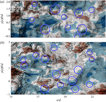
Figure 18 displays enlarged views of  $u$-fluctuations within the rectangles marked in figures 17(a) and 17(b). Also shown in figure 18 are the in-plane velocity vectors resulting from subtracting the local mean velocity from the flow field. When a Galilean decomposition is considered in an axial–azimuthal plane, the vortical structures moving with a velocity equal to the mean velocity are highlighted with a zero velocity vector (since the mean azimuthal velocity is zero in axisymmetric jets). Patterns of circular streamlines (demarcated by circles) are visible, which in some cases appear in pairs. Here, in figure 18, for demonstration purposes, only clear circular streamline regions are marked, while other less clear (unmarked) circular streamline regions are present. Similar circular patterns of velocity vectors, called hairpin vortex signatures, have been reported in wall-bounded turbulent flows (e.g. Tomkins & Adrian Reference Tomkins and Adrian2003; Lee & Sung Reference Lee and Sung2011). Here, we call them hairpin eddy signatures to avoid confusion between the vortex rings in the near field and ESs in the fully turbulent region. These hairpin eddy signatures in wall-bounded turbulence are known to be cross-sections through the two legs of three-dimensional hairpin ESs whose spanwise head is parallel to the wall. Hairpin-like ESs have also been reported in axisymmetric turbulent jets using time-resolved stereo PIV (Matsuda & Sakakibara Reference Matsuda and Sakakibara2005) and scanning tomographic PIV data (Casey, Sakakibara & Thoroddsen Reference Casey, Sakakibara and Thoroddsen2013). In general, the orientation of a hairpin-like ES in an axisymmetric jet is such that its legs are located near the jet axis while its head points away from the jet axis (Suto et al. Reference Suto, Matsubara, Kobayashi, Watanabe and Matsudaira2004).
Hairpin eddy signatures shown on snapshots of axial velocity fluctuations at (a)  $y(x)/y_{0.5}(x)=0.6$ and (b)
 $y(x)/y_{0.5}(x)=1$ for the regions demarcated by the rectangles in figure 17. In-plane velocity vectors are shown at every fifth grid point in the axial direction and all the grid points in the azimuthal direction.

Another important feature of a hairpin eddy signature is that it is often observed on the border of high-speed and low-speed regions. Indeed, this is the case in figure 18. This observation is explained by induction of a positive axial velocity region inside a hairpin ES and two negative axial velocity regions on both sides of it (discussed further in § 5). When a single hairpin ES is found in the flow (e.g. at  $(x/d,y \theta /d)=(16,1.5)$ in figure 18b), the induced positive axial velocity field can be seen clearly between the hairpin eddy signatures, one of which is clockwise while the other one is anticlockwise. However, the ESs often appear in groups and their total induced flow field is the result of interactions of several ESs moving together in the flow. Although it is expected to find two counter-rotating eddy patterns created by the intersection of the cut plane with the eddy legs (Lee et al. Reference Lee, Sung and Adrian2019), this is often not the case due to grouping of ESs and asymmetry of the ESs (i.e. one leg is shorter and both legs are not shown in an axial–azimuthal plane). The existence of C-shaped ESs in the fully turbulent region of jets is evident from the study of Matsuda & Sakakibara (Reference Matsuda and Sakakibara2005). They reported ESs in both instantaneous and conditionally averaged flow fields. Using the linear stochastic estimation, they extracted a conditionally averaged C-shaped ES in the turbulent jet featured by a high-speed region between the legs of the eddy and low-speed regions on both sides of the legs. The hairpin eddy signatures observed in figure 18 seem to indicate the circular flow pattern created by the legs of these ESs in instantaneous flow fields reported by Matsuda & Sakakibara (Reference Matsuda and Sakakibara2005). The hairpin ES in wall-bounded turbulence induces a low-speed region between its legs as opposed to the ES observed in the turbulent round jet with a high-speed region induced between its legs.
5. Synthetic flow fields and a conceptual model
The DNS flow fields displayed oblique VLSMs in the axial–azimuthal plane. It was hypothesized that the appearance of anticorrelation lobes in the experimental azimuthal  $R_{vl}$ maps in both
 $\tau$- and
 $\Delta s$-directions (figure 13) stems from the obliqueness of the VLSMs. To evaluate this hypothesis, two synthetic flow fields, consisting of only VLSMs, are generated to model the jet flow in a two-dimensional axial–azimuthal unwrapped plane. The first flow field is populated with structures that consist of axially aligned elongated high-speed regions flanked on either side by low-speed regions of the same length and width. This structure for the VLSM is inspired from the experimental azimuthal two-point correlation maps displayed in figure 4. A representative axially aligned synthetic structure is shown in figure 19(a). The lengths of the structures follow a normal distribution with a mean
 $l_x=10l_s$, where
 $l_s$ is half of the structure width, as displayed on figure 19(a). Hundreds of these structures are randomly arranged to form a flow field with axial and azimuthal lengths of
 $L_x=200l_s$ and
 $L_s=10l_s$, respectively.
Two types of synthetic (analytical) structures used to model the synthetic flow field: (a) an axially aligned structure, and (b) an oblique structure at an angle of  $30^\circ$ to the jet axis. (c,d) Azimuthal correlation maps corresponding to the synthetic flow fields modelled with (c) axially aligned structures and (d) oblique structures. Solid lines in panels (c,d) represent contour levels of
 $R_{uu}=0.2$, 0.6 and 0.9, and dashed lines correspond to contour levels of
 $R_{uu}= -0.3 \text { and } {-}0.1$.

The second synthetic flow field comprises hundreds of oblique structures (with the same length as the axially aligned ones); half of these oblique structures make positive angles with the main flow direction following a normal distribution with a mean  $\theta _p=30^\circ$, while the orientation of the other half is
 $\theta _n=-\theta _p$. One of these oblique structures with a positive angle is displayed in figure 19(b). Two hypothetical sensors are schematically shown close to the axially aligned and oblique structures. One can see that when the axially aligned structure passes the sensor (in the
 $x$-direction), either the high-speed or the low-speed region is measured by the sensor. However, in the case of oblique structures, the sensor measures both the high-speed and low-speed regions consecutively as projected by the horizontal dashed line, leading to negative autocorrelation lobes in the
 $\Delta x$-direction.
Azimuthal two-point correlations associated with the first and second synthetic flow fields are calculated and averaged over dozens of synthetic flow fields and shown in figures 19(c) and 19(d), respectively. Although the length scales of the features used to populate the first and second synthetic flow fields are the same, a significant difference is observed between the length scales associated with the correlation contour value  $R_{uu}=0.2$. For the axially aligned case, the correlation contours at
 $\Delta s=0$ approximately represent the axial span of the structure. However, for the oblique case, the correlation contours at
 $\Delta s=0$ cross zero at
 $\Delta x/l_s \approx {\pm }0.8$, which is substantially smaller than the axial length of the structures used to populate the synthetic flow. Notably, in the correlation contours corresponding to the oblique structures case, anticorrelation lobes flank the positive correlation main lobe in the
 $\Delta x$-direction. This is a similar pattern to that observed for the experimental VLSM component of the correlations displayed in figure 13. Although the anticorrelation regions in the experimental correlation maps are weaker, this similarity seems to support the hypothesis of the importance of oblique VLSMs in the turbulent round jet. These results do not imply that the oblique structures are the only form of VLSMs in the round jet flow, but rather they support the hypothesis regarding their general shape and importance. To obtain the probability of all the possible forms of VLSMs (streaks, rings and helices), a conditional averaging type of analysis to educe VLSMs similar to that conducted by Hutchins et al. (Reference Hutchins, Monty, Ganapathisubramani, Ng and Marusic2011) is required and is the subject of ongoing work.
A conceptual model is proposed for the coherent structures in the turbulent round jet. This model is presented in a stochastic sense and holds only the salient features of the VLSMs in an instantaneous flow field. The DNS instantaneous flow fields revealed signatures of ESs on the boundaries between high-speed and low-speed regions. Based on the  $\gamma _L^2$ spectra, a physical aspect ratio of
 $1.2:1:1$ for the ESs was proposed in § 3.2. This is compatible with the visualization of hairpin-like ESs in both jet flows and wall-bounded flows that exhibit similar spans in the axial, radial and azimuthal directions for ESs. Therefore, contrary to wall-bounded flows, where packets of eddies are proposed as hierarchical building blocks of coherent structures (Baars & Marusic Reference Baars and Marusic2020), in the round jets single eddies are the hierarchical components shaping larger coherent features.
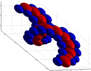
An ES together with its induced flow field is displayed schematically in figure 20(a,b). Here the ES is represented by a C-shaped tube, while an induced high-speed and two induced low-speed regions are shown by red and blue regions, respectively. Note that the eddy presented here belongs to one eddy hierarchy level, and eddies of varying sizes are present in the flow. When the VLSMs resulting from concatenation of several eddies are considered, only the largest ESs are shown for clarity. The largest ESs concatenate to form VLSMs. It was shown using both DNS data and synthetic flow fields that the VLSMs, when viewed in an unwrapped axial–azimuthal cone, form oblique angles with the  $x$-axis. This implies that the VLSMs are stochastically helical structures in a three-dimensional field of a turbulent round jet. The VLSMs are illustrated schematically in an axial–azimuthal two-dimensional plane in figure 20(c). A three-dimensional isotropic view of a VLSM is presented in figure 20(d). The length of these helical structures is not clear and can be very short, forming oblique structures, or very long, forming a clear helix. The proposed simplified model is arguably the simplest representation that explains the results presented here. Other equally valid models to explain these observations may exist.
Schematics of coherent structures. (a) Isometric view of an isolated ES (shown with the green curved tube) and high-speed (red ellipsoid) and low-speed (blue ellipsoids) regions induced by the eddies. (b) Top view of panel (a). (c) Helical concatenation of eddies forming a VLSM, where the structures are shown on an unwrapped axial–azimuthal plane. (d) A helical VLSM formed by concatenation of several ESs.

6. Concluding remarks
Two-point measurements were conducted with separations between the sensors in both radial and azimuthal directions to assess coherent structures in axisymmetric turbulent jets. The measurements were made in the intermediate field of a turbulent round jet in the range  $x/d=15\text {--}25$ and over a range of Reynolds numbers from
 $Re_d=10\,000$ to
 $50\,000$. Radial two-point correlations displayed no sign of a
 $Re_d$ effect on the large-scale coherent structures. The average inclination angle (with respect to the
 $x$-axis) associated with the coherent structures was estimated using the radial two-point correlations. It was shown that this angle decreases with the radial distance for all
 $Re_d$. Azimuthal two-point correlations indicate a negative correlation lobe in the azimuthal distance range
 $\Delta s/y_{0.5}>0.6$ alongside the main positive lobe. A similar pattern has been reported in other turbulent shear flows and is attributed to a stochastically dominant configuration of the axial flow induced by ESs. When normalized with
 $y_{0.5}$, the size of the structures in the azimuthal correlation did not display a dependence on
 $Re_d$.
The LCS was computed using data from the two-point synchronized measurements with sensor separations in both radial and azimuthal directions. The radial linear coherence spectra revealed a hierarchical ES in the turbulent round jet associated with the outer-scaled wavelength range  $\lambda _x/y_{0.5} \approx 0.2\text {--}4$. The ESs in the shear layer of the jet are shown to be geometrically self-similar, with a stochastic axial–radial aspect ratio of
 . The azimuthal linear coherence spectra (
 $\gamma _L^2$ against
 $\Delta s/y_{0.5}$ and
 $\lambda _x/y_{0.5}$) showed that only the small ESs associated with the wavelength domain
 $\lambda _x/y_{0.5} \approx 0.2\text {--}0.8$ are self-similar, with an axial–azimuthal aspect ratio that is equal to the radial–azimuthal aspect ratio
 . Consequently, a physical aspect ratio of
 $1.2:1:1$ in the axial, radial and azimuthal directions was proposed for the hierarchical ESs in the turbulent round jet. In both radial and azimuthal experimental LCS, the coherence contours become approximately wavelength-independent for
 $\lambda _x/y_{0.5}>4$. We conjectured that this wavelength domain is associated with the VLSMs. This wavelength was used to separate the VLSMs and ESs in the jet, and the VLSM and ES components of two-point correlations were obtained. Two negative correlation lobes appeared in the
 $\tau$-direction of the VLSM correlation maps for both radial and azimuthal correlations. These anticorrelation lobes do not exist in the original two-point correlation maps due to superposition of the VLSMs and ESs. The contribution of the VLSMs was estimated by integrating the VLSM component of the
 $u$-energy spectrum. It was shown that, depending on the radial location, VLSMs constitute between
 $30\,\%$ and
 $80\,\%$ of the total
 $u$-turbulence intensity of the jet. Comparing these values with an estimated maximum value of
 $16\,\%$ in turbulent boundary layers underlines the importance of VLSMs in the dynamics of turbulent round jets.
Instantaneous views of  $u$-fluctuations in axial–azimuthal unwrapped cones from DNS suggest the presence of oblique VLSMs in the intermediate field of the jet, which are identified as high-speed regions flanked by low-speed regions on either side in the azimuthal direction. Overlay of the in-plane velocity vectors on the
 $u$-fluctuation contours reveals two-dimensional vortex-like regions often located at the boundaries between the high-speed and low-speed regions. We attribute these hairpin eddy signatures to the ESs, which induce a high-speed region between and low-speed regions outside of their legs. These ESs appear in groups forming oblique VLSMs.
In order to examine the effect of obliqueness of the VLSMs on the two-point correlations, two two-dimensional axial–azimuthal synthetic flow fields were generated. In the first one, the VLSMs were modelled with axially aligned structures; while in the second, synthetic flow field oblique structures were used to populate the flow. The correlation map associated with the synthetic flow field populated with the oblique structures qualitatively resembles the VLSM component of correlation maps from experiment, reinforcing the observation that the VLSMs are predominantly oblique in an axial–azimuthal plane. This implies the significance of helical structures as the VLSMs in the axisymmetric turbulent jet. Finally, in accordance with the experimental and DNS results, as well as the synthetic flow fields, an idealized model for coherent structures in turbulent round jets was proposed in which ESs concatenate and form very-large-scale helical structures.
Acknowledgements
The authors would like to give special thanks to Professor D.-H. Shin (formerly University of Edinburgh, now Korea Advanced Institute of Science and Technology), V. Aparece-Scutariu (Ph.D. student, University of Edinburgh) and Professor E.S. Richardson (University of Southampton) for providing access to and assisting with the use of their DNS data.
Funding
Financial support from the Natural Sciences and Engineering Research Council of Canada (NSERC) is gratefully acknowledged.
Declaration of interests
The authors report no conflict of interest.
Appendix A
The VLSM and ES components of the  $u$-fluctuations were separated in both experimental and DNS data using second-order Butterworth filters. The effect of the filter order on the ES and VLSM components of the correlations in the experimental data is examined here. Figure 21(a) shows an example premultiplied
 $u$-energy spectrum together with the VLSM and ES components obtained with Butterworth filters of orders
 $N=1$, 2 and 4. Evidently, increasing the filter order leads to a sharper transition at the separating wavelength (
 $\lambda _x=4y_{0.5}$) for both VLSM and ES components. The ES and VLSM components of the correlations associated with these filters are shown in figures 21(a) and 21(b), respectively. One can see that, in both
 $R_{es}$ and
 $R_{vl}$, the main positive correlation lobe is flanked by negative anticorrelation lobes for
 $N=1$, 2 and 4. Moreover, the negative correlation lobes seem to become more negative with increasing
 $N$. A Gaussian filter was also used to separate the VLSMs and ESs (not shown here for clarity), which yielded filtered correlations with negative lobes similar to those from a Butterworth filter with
 $N=1$. These results show that, although changing the order of the filter modifies the magnitude of the negative lobe, the filtered correlations are qualitatively similar. Therefore, the filter type and order do not affect our conclusions with regard to the coherent structures.
(a) Effect of the filter order ( $N=1,2,4$) on the ES and VLSM components of the
 $u$-premultiplied energy spectrum shown in figure 10(b). (b) Associated ES component of correlations
 $R_{es}$. (c) Associated VLSM component of correlations
 $R_{vl}$. Arrows show increase in the filter order in all panels.

Appendix B
A conceptual reconstruction of the  $\gamma _L^2$ spectra is introduced here to help comprehend the proposed spectral boundary between ESs and VLSMs inferred from the LCS. Samie et al. (Reference Samie, Lavoie and Pollard2020) showed that hierarchical ESs are embedded in the turbulent jet. Here, the LCS is reconstructed conceptually using four discrete hierarchy levels (ESs of four different sizes) as shown schematically in figure 22(a) in the (
 $x,y$)-space. The number of hierarchy levels is chosen arbitrarily here for illustration of the conceptual
 $\gamma _L^2$ spectra reconstruction. The inclination angle of the eddies with respect to the jet axis is neglected, since a consistent phase shift is irrelevant in the context of the LCS and spectra.
Conceptual reconstruction of the LCS. (a) Four schematic eddy hierarchy structures and associated (b)  $\gamma _L^2$ spectra and (c) coherence spectrogram. (d) Coherence spectrogram for a realistic flow that comprises a continuous spectrum of eddy sizes (as opposed to four discrete eddy hierarchy levels).

Each ES in figure 22(a) represents a large number of eddies of that size, which are randomly distributed around the jet centreline. Associated with each of these hierarchy levels is a minimum wavelength that is proportional to the axial length of the representative eddy belonging to that level ( $\lambda _i$,
 $i=1,\ldots ,4$), below which the energy spectrum corresponding to that hierarchy level is zero.
Consider two probes that are located in the flow and simultaneously measure the axial velocity field generated by these ESs. The white small square in figure 22(a) represents a fixed probe while the blue circles (with different shadings) show the location of the second probe (traversing probe) at four different positions. When the traversing probe is located at point 1, both probes simultaneously measure the velocity field associated with the largest ESs (first hierarchy level) only, yielding a coherence that is non-zero for  $\lambda _x>\lambda _1$ as shown by the light-coloured lines in figure 22(b). Note that
 $\gamma _L^2$ is non-zero for
 $\lambda _x>\lambda _1$ due to the random repetition of the eddies belonging to the first hierarchy level in the axial direction.
Moving the traversing probe to point 2, velocity fields of the first hierarchy and the second hierarchy eddy levels are superposed. This results in the superposition of the coherence from these two hierarchy levels corresponding to the minimum wavelengths  $\lambda _1$ and
 $\lambda _2$, where
 $\lambda _1>\lambda _2$. Therefore, the coherence contribution from the second hierarchy level is superposed on that from the first hierarchy level, resulting in an increase of coherence level where they overlap (
 $\lambda _x>\lambda _1$) and producing non-zero coherence for
 $\lambda _2<\lambda _x<\lambda _1$ as shown in figure 22(b). Continuing this process for points 3 and 4 generates coherence values that superpose over the overlapping wavelengths as shown in figure 22(b) (lines 3 and 4).
Samie et al. (Reference Samie, Lavoie and Pollard2020) verified the assumption of the superposition of the coherence using a synthetic flow field. If the LCS are plotted against  $\Delta y$ and
 $\lambda _x$, the
 $\gamma _L^2$ spectrogram is obtained as shown in figure 22(c). It is not difficult to show that, by increasing the number of hierarchy levels, the staircase-like spectrogram corresponding to four hierarchy levels approaches a smooth spectrogram for a realistic flow comprising a continuous spectrum of eddy sizes. This is shown in figure 22(d). Note that, when the eddy hierarchy levels are not discrete, the wavelength associated with each of them is not recognizable on the
 $\gamma _L^2$ spectra. However, the wavelength corresponding to the largest representative ES (
 $\lambda _1$) is an exception and is still visible as the wavelength where a transition in the behaviour of the
 $\gamma _L^2$ contours occurs. According to the experimental
 $\gamma _L^2$ spectra, this wavelength is
 $\lambda _1/y_{0.5} \approx 4$ for the turbulent round jet. Based on the conceptual reconstruction of the
 $\gamma _L^2$ spectra, one can see that the LCS in the wavelength domain
 $\lambda _x<\lambda _1$ is constructed by ESs, while the domain corresponding to
 $\lambda _x>\lambda _1$ is associated with the repetition of ESs (i.e. VLSMs). Therefore, the wavelength associated with the start of the wavelength-independent spectral domain in the LCS is adopted as the lower spectral limit for the VLSMs and the upper spectral limit of the ESs.