1 Introduction
Disturbances in the oncoming flow, loosely referred to as free-stream turbulence (FST), plays a crucial role in laminar–turbulent transition in boundary layers. In the presence of low-level FST, transition is caused by amplification of Tollmien–Schlichting waves (Kachanov Reference Kachanov1994), which correspond to discrete modes of the Orr–Sommerfeld (O–S) equation. FST influences what is referred to as natural transition through receptivity (Duck, Ruban & Zhikharev Reference Duck, Ruban and Zhikharev1996; Wu Reference Wu2001; Saric, Reed & Kerschen Reference Saric, Reed and Kerschen2002). If the FST level exceeds a critical value about 1 %, low-frequency streaks appear in the boundary layer (Klebanoff Reference Klebanoff1971; Kendall Reference Kendall1990; Westin et al. Reference Westin, Boiko, Klingmann, Kozlov and Alfredsson1994), and they amplify and break down via a secondary instability (Matsubara & Alfredsson Reference Matsubara and Alfredsson2001). This is the so-called bypass transition route (Morkovin Reference Morkovin1984). In either of these two scenarios, the transition location depends on the intensity (and possibly other characteristics) of the FST, and predicting such dependence is the ultimate goal of transition research. Clearly, characterizing how FST enters the boundary layer, or how the boundary layer responds to FST, is a crucial first step.
Since the oncoming free stream is often uniform and the disturbances are usually of small amplitude, FST can be represented as a supposition of acoustic, vortical and entropy modes (Kovasznay Reference Kovasznay1953). The way by which each of these modes impacts the boundary layer is quite different. An acoustic mode represents a pressure fluctuation, through which it drives velocity fluctuations in the boundary layer. In the generic case where the wavelength and frequency are comparable with the boundary-layer thickness
 ${\it\delta}^{\ast }$
and
 $U_{\infty }/{\it\delta}^{\ast }$
respectively (where
 $U_{\infty }$
is the free-stream velocity), the induced signature is represented by the eigenfunction of the acoustic-mode branch of the continuous spectra of the linearized disturbance equations. (In the long-wavelength limit, the velocity fluctuation may concentrate in a thin viscous Stokes layer adjacent to the wall.)
Free-stream vortical disturbances (FSVD) represent weak vorticity being advected by the uniform background flow so that their phase speeds are nearly equal to the velocity of the latter, and there is no pressure fluctuation at leading order. The process of FSVD entering the boundary layer, which we shall refer to as entrainment, is rather subtle. FSVD with the characteristic streamwise wavelength being comparable with the spanwise wavelength,
 ${\it\Lambda}$
say, was considered first by Gulyaev et al. (Reference Gulyaev, Kozlov, Kuznetsov, Mineev and Sekundov1989). They showed that in the region at an
 $O({\it\Lambda})$
distance to the leading edge, the induced perturbation is governed by the linearized boundary-layer equations, and its streamwise velocity increases with the streamwise distance. Leib, Wundrow & Goldstein (Reference Leib, Wundrow and Goldstein1999) considered FSVD whose streamwise wavelength is longer than the spanwise length scale
 ${\it\Lambda}$
by a factor
 $R_{{\it\Lambda}}$
(the Reynolds number based on
 ${\it\Lambda}$
). In the region at an
 $O({\it\Lambda}R_{{\it\Lambda}})$
distance to the leading edge, the induced motion is governed by the so-called linearized boundary-region equations (Kemp Reference Kemp1951), and most significantly, its streamwise velocity acquires a magnitude of
 $O(R_{{\it\Lambda}}{\it\epsilon})$
, much greater than
 ${\it\epsilon}$
, the intensity of FSVD. The boundary-layer fluctuations therefore take on the appearance of streaks. The linear theory of Leib et al. (Reference Leib, Wundrow and Goldstein1999) for incompressible flows was extended by Ricco & Wu (Reference Ricco and Wu2007) to compressible boundary layers and by Ricco, Luo & Wu (Reference Ricco, Luo and Wu2011) to the case where FSVD are of sufficient intensity (i.e.
 ${\it\epsilon}=O(R_{{\it\Lambda}}^{-1})$
) to generate streaks with an
 $O(1)$
streamwise velocity. The boundary-layer responses to steady free-stream perturbations in the form of wall-normal and streamwise vorticity have also been studied with a broadly similar mathematical framework by Crow (Reference Crow1966), Goldstein, Leib & Cowley (Reference Goldstein, Leib and Cowley1992), Goldstein & Leib (Reference Goldstein and Leib1993) and Wundrow & Goldstein (Reference Wundrow and Goldstein2001). See also the review by Goldstein (Reference Goldstein2014). In all these analyses, non-parallelism plays a leading-order role, which is expected since the streamwise wavelength of the perturbation is comparable with the length scale of the underlying base flow.
Recently, Dong & Wu (Reference Dong and Wu2013) considered the boundary-layer response to FSVD with wavelength comparable with the local boundary-layer thickness. Interestingly, despite the relatively short wavelength, non-parallelism appears at leading order in the edge layer, which is located at the outer edge of the boundary layer, and controls the entrainment process. When non-parallelism is neglected artificially, the disturbance equations reduce to the O–S and Squire equations. Since continuous modes of these equations have the same phase speeds as free-stream vortical disturbances, it has been suggested that each continuous mode represents a Fourier component in the vortical disturbance with its eigenfunction characterizing the distribution of the perturbation entrained into the boundary layer (Grosch & Salwen Reference Grosch and Salwen1978). This interpretation was examined by Dong & Wu (Reference Dong and Wu2013). They noted that continuous modes exhibit two peculiar features: ‘entanglement of Fourier components’ and ‘abnormal anisotropy’. The first refers to the fact that the eigenfunction of a continuous mode consists of two components with wall-normal wavenumbers
 $\pm k_{2}$
with the ratio of their respective amplitudes being fixed by the boundary layer, while the second refers to the consequence that for low-frequency modes, the presence of the boundary layer forces the streamwise velocity in the free stream to be much greater than the transverse velocities. Both features are non-physical because the spectral composition of a free-stream disturbance should be determined by the conditions upstream rather than by the boundary layer underneath, and both can be attributed to neglecting non-parallelism, which affects entrainment at leading order as mentioned above. Thus unlike discrete modes, continuous modes have no physical meaning, and despite the fact that continuous modes and convected vortical disturbances have the same phase speed, the eigenfunction of the former does not represent the distribution of the boundary-layer fluctuation induced by the latter, contrary to the usual interpretation of continuous modes (Grosch & Salwen Reference Grosch and Salwen1978).
The findings of Dong & Wu (Reference Dong and Wu2013) have important implications for a crucial issue in direct numerical simulations (DNS) of bypass transition, namely, the specification of an appropriate inlet condition. Jacobs & Durbin (Reference Jacobs and Durbin2001) suggested that the inlet condition can be specified in terms of a superposition of continuous spectra. This practice has been followed in subsequent studies of bypass transition (Brandt, Schlatter & Henningson Reference Brandt, Schlatter and Henningson2004; Zaki & Durbin Reference Zaki and Durbin2005; Liu, Zaki & Durbin Reference Liu, Zaki and Durbin2008). It has also been adopted to simulate receptivity and transition in three-dimensional boundary layers as well as in boundary layers over a concave wall, where transition is caused by cross-flow and Görtler instabilities, respectively. However, the results of Dong & Wu (Reference Dong and Wu2013) imply that an inlet condition constructed in this manner does not provide a correct link between FST and the disturbance that it induces in the boundary layer, and is therefore inappropriate.
In this paper, we extend the analysis of Dong & Wu (Reference Dong and Wu2013) to free-stream disturbances which have a characteristic wavelength comparable with the width of the edge layer, much shorter than the
 $O({\it\delta}^{\ast })$
wavelength considered in the earlier work. The analysis will be performed for compressible boundary layers, and so a further extension consists of including the effects of compressibility. Some preliminary results were published in Dong & Wu (Reference Dong and Wu2015). The present study was prompted by two main motivations. Firstly, free-stream disturbance usually consists of a broadband of components in spectral (wavenumber and frequency) space. For the purpose of investigating bypass transition and receptivity, it is important to calculate the boundary-layer signature induced by these components. The short-wavelength scaling to be adopted is appropriate as it turns out to be more general in that the results in the previous paper can be recovered in an appropriate limit, and the solution for the boundary-layer signature remains valid for a broadband of frequencies and wavenumbers. Secondly, in the case of compressible boundary layers some rather peculiar behaviours of the continuous modes have been noted by Joo & Durbin (Reference Joo and Durbin2010). The present analysis intends to offer a proper explanation for those features, and to demonstrate the differences between the continuous modes and the disturbance entrained into the boundary layer.
The rest of the paper is planned as follows. In § 2, we formulate the problem by writing down the linearized compressible N–S equations, which govern small-amplitude disturbances superimposed on a general boundary-layer flow. In § 3, the entrainment of FSVD is analysed in the appropriate mathematical setting, the linearized N–S equations, which include the non-parallelism associated with the gradual thickening of the boundary layer. We show that the entrainment is influenced, to leading order, by the non-parallel-flow effect. Appropriate solutions are constructed, and their main characteristics are discussed. In § 4, we revisit the problem of continuous spectra for compressible boundary layers by removing from the linearized N–S equations the terms representing non-parallelism (but retaining the viscous terms). Numerical solutions to the resulting equations reveal, in addition to the two non-physical features present in the incompressible case, yet another one, entanglement of the vortical and entropy modes. The high Reynolds number asymptotic analysis of continuous spectra is then presented for the present shorter-wavelength scaling. The ‘entanglements’ mentioned above are shown to be a consequence of neglecting the non-parallel-flow effect. With this effect being properly taken into account, none of the non-physical features arise. A summary of the main results and a discussion of their implications are given in § 5.
2 Small-amplitude disturbances in boundary-layer flows: linearized compressible Navier–Stokes equations
We consider the compressible boundary layer that forms over a semi-infinite plate. The flow will be described by the Cartesian coordinate system
 $(x,y,z)$
, where
 $x$
,
 $y$
and
 $z$
denote the coordinates in the streamwise, wall-normal and spanwise directions respectively, and they are normalized by a characteristic boundary-layer thickness
 ${\it\delta}^{\ast }$
. The free-stream velocity
 $U_{\infty }$
and
 ${\it\delta}^{\ast }/U_{\infty }$
will be taken as the reference speed and time respectively. The Reynolds number
 $R$
and Mach number
 $M$
are defined as
 $$\begin{eqnarray}R=U_{\infty }{\it\delta}^{\ast }/{\it\nu}_{\infty }^{\ast },\quad M=U_{\infty }/a_{\infty },\end{eqnarray}$$
with
 ${\it\nu}_{\infty }^{\ast }$
being the kinematic viscosity of the fluid and
 $a_{\infty }$
the speed of sound in the free stream. The fluid is assumed to be a perfect gas with a ratio of specific heats
 ${\it\gamma}$
.
2.1 The base flow
The non-dimensionalized velocity field
 $\boldsymbol{U}_{B}$
, pressure
 $P_{B}$
, temperature
 $T_{B}$
and density
 $R_{B}$
of the base flow may be written as
 $$\begin{eqnarray}(\boldsymbol{U}_{B},P_{B},T_{B},R_{B})=(U(\bar{x},y),R^{-1}V(\bar{x},y),0,1/({\it\gamma}M^{2}),T,1/T),\end{eqnarray}$$
where the base flow evolves on the slow streamwise variable
 $$\begin{eqnarray}\bar{x}=x/R.\end{eqnarray}$$
The steady boundary-layer equations governing the base flow admit the similarity solution (Stewartson Reference Stewartson1964)
 $$\begin{eqnarray}U=F^{\prime }({\it\eta}),\quad V=(2\bar{x})^{-1/2}T({\it\eta}_{c}F^{\prime }-F),\quad T=T({\it\eta}),\end{eqnarray}$$
where the prime denotes differentiation with respect to the argument,
 $$\begin{eqnarray}{\it\eta}=(2\bar{x})^{-1/2}\int _{0}^{y}\frac{\text{d}y}{T},\quad {\it\eta}_{c}=\frac{1}{T}\int _{0}^{{\it\eta}}T({\it\eta})\,\text{d}{\it\eta}.\end{eqnarray}$$
It follows that
 $$\begin{eqnarray}\frac{\partial {\it\eta}}{\partial \bar{x}}=-{\it\eta}_{c}/(2\bar{x}),\quad \frac{\partial {\it\eta}}{\partial y}=1/(T\sqrt{2\bar{x}}).\end{eqnarray}$$
The functions,
 $F$
and
 $T$
, satisfy the equations
 $$\begin{eqnarray}\left.\begin{array}{@{}c@{}}\displaystyle F^{\prime \prime \prime }+\frac{FF^{\prime \prime }}{K}+\frac{K^{\prime }T^{\prime }F^{\prime \prime }}{K}=0,\\ \displaystyle T^{\prime \prime }+\frac{\mathit{Pr}\,FT^{\prime }}{K}+\frac{K^{\prime }\bar{T}^{\prime 2}}{K}+\mathit{Pr}({\it\gamma}-1)M^{2}(F^{\prime \prime })^{2}=0,\end{array}\right\}\end{eqnarray}$$
where we have put
 $K={\it\mu}(T)/T$
and
 $\mathit{Pr}$
is the Prandtl number. The system of coupled equations above is to be solved subject to the boundary conditions
 $$\begin{eqnarray}F(0)=F^{\prime }(0)=0,\quad F^{\prime }\rightarrow 1\quad \text{as}~{\it\eta}\rightarrow \infty ,\end{eqnarray}$$
and
 $$\begin{eqnarray}T^{\prime }(0)=0,\quad T\rightarrow 1\quad \text{as}~{\it\eta}\rightarrow \infty\end{eqnarray}$$
if the wall the insulated, or
 $$\begin{eqnarray}T^{\prime }(0)=T_{w},\quad T\rightarrow 1\quad \text{as}~{\it\eta}\rightarrow \infty\end{eqnarray}$$
if the wall is isothermal with a temperature
 $T_{w}$
. The coupled system (2.7) has to be solved, but for
 $\mathit{Pr}=1$
, the temperature profile is related to
 $U$
via
 $$\begin{eqnarray}T=1+{\textstyle \frac{1}{2}}({\it\gamma}-1)M^{2}(1-U^{2}),\end{eqnarray}$$
and hence the equations become decoupled.
As
 ${\it\eta}\rightarrow \infty$
, both
 $U$
and
 $T$
approach unity exponentially,
 $$\begin{eqnarray}U\sim 1-\frac{\hat{a}}{{\it\eta}-{\it\beta}}\text{e}^{-(1/2)({\it\eta}-{\it\beta})^{2}},\quad T\sim 1-\frac{\hat{b}}{{\it\eta}-{\it\beta}}\text{e}^{-(\mathit{Pr}/2)({\it\eta}-{\it\beta})^{2}},\end{eqnarray}$$
where
 $\hat{a}$
and
 $\hat{b}$
are constants, and
 $$\begin{eqnarray}{\it\beta}=\int _{0}^{\infty }(1-U)\,\text{d}{\it\eta}.\end{eqnarray}$$
More precisely, the streamwise velocity and the temperature for
 ${\it\eta}\gg 1$
can be approximated as
 $$\begin{eqnarray}U\rightarrow 1-\mathscr{U}_{D},\quad T\rightarrow 1-\mathscr{T}_{D},\end{eqnarray}$$
where
 $$\begin{eqnarray}\mathscr{U}_{D}=\hat{a}\int _{{\it\eta}}^{\infty }\text{e}^{-(1/2)({\it\eta}-{\it\beta})^{2}}\,\text{d}{\it\eta},\quad \mathscr{T}_{D}=\mathit{Pr}\,\hat{b}\int _{{\it\eta}}^{\infty }\text{e}^{-(1/2)\mathit{Pr}({\it\eta}-{\it\beta})^{2}}\,\text{d}{\it\eta}.\end{eqnarray}$$
2.2 Perturbations in the boundary layer
Suppose that the base flow (2.2) is perturbed by a small-amplitude disturbance of the travelling-wave form,
 $$\begin{eqnarray}(\tilde{u} ,\tilde{v},\tilde{w},\tilde{p},\tilde{{\it\theta}},\tilde{{\it\rho}})={\it\epsilon}(u(\bar{x},y),v(\bar{x},y),w(\bar{x},y),p(\bar{x},y),{\it\theta}(\bar{x},y),{\it\rho}(\bar{x},y))\text{e}^{\text{i}(k_{1}x+k_{3}z-{\it\omega}t)}+\text{c.c.},\end{eqnarray}$$
where
 ${\it\omega}$
,
 $k_{1}$
and
 $k_{3}$
denote the frequency, streamwise and spanwise wavenumbers respectively, and the magnitude
 ${\it\epsilon}\ll 1$
. The disturbance may represent (discrete or continuous) modal fluctuations or the response forced by external perturbations. Note that the normal distribution (i.e. the shape) of the disturbance depends on the slow variable
 $\bar{x}$
. It follows from substitution of (2.16) into the N–S equations and linearization that
 $(u,v,w,p,{\it\theta},{\it\rho})$
satisfy the linearized compressible N–S equations,
 $$\begin{eqnarray}\displaystyle \text{i}k_{1}u+v_{y}+\text{i}k_{3}w & = & \displaystyle -T[\text{i}(k_{1}U-{\it\omega}){\it\rho}-(T_{y}/T^{2})v]-u_{\bar{x}}/R\nonumber\\ \displaystyle & & \displaystyle -\,T[\mathscr{L}_{1}{\it\rho}+(1/T)_{\bar{x}}u+(U_{\bar{x}}+V_{y}){\it\rho}]/R,\end{eqnarray}$$
 $$\begin{eqnarray}\displaystyle \text{i}(k_{1}U-{\it\omega})u+U_{y}v & = & \displaystyle T[-\text{i}k_{1}p+p_{\bar{x}}/R+{\rm\Delta}u/R]-(\mathscr{L}_{1}u+U_{\bar{x}}u)/R\nonumber\\ \displaystyle & & \displaystyle +\,T[\text{i}k_{1}({\it\mu}S+{\it\mu}^{\prime }T_{y}v)+(U_{y}{\it\mu}^{\prime }{\it\theta})_{y}-(UU_{\bar{x}}+VU_{y}){\it\rho}]/R,\qquad \quad\end{eqnarray}$$
 $$\begin{eqnarray}\displaystyle \text{i}(k_{1}U-{\it\omega})v & = & \displaystyle T[-p_{y}+{\rm\Delta}v/R]-(\mathscr{L}_{1}v+V_{y}v)/R-V_{\bar{x}}u/R^{2}\nonumber\\ \displaystyle & & \displaystyle +\,T[{\it\mu}S_{y}/3+{\it\mu}^{\prime }(T_{y}v_{y}+\text{i}k_{1}U_{y}{\it\theta})-2{\it\mu}^{\prime }T_{y}S]/R\nonumber\\ \displaystyle & & \displaystyle +\,T[(V_{y}{\it\mu}^{\prime }{\it\theta})_{y}-(UV_{\bar{x}}+VV_{y}){\it\rho}]/R^{2},\end{eqnarray}$$
 $$\begin{eqnarray}\displaystyle \text{i}(k_{1}U-{\it\omega})w & = & \displaystyle T[-\text{i}k_{3}p+{\rm\Delta}w/R]-\mathscr{L}_{1}w/R+T(\text{i}k_{3}S+{\it\mu}^{\prime }T_{y}\text{i}k_{3}v)/R,\end{eqnarray}$$
 $$\begin{eqnarray}\displaystyle \text{i}(k_{1}U-{\it\omega}){\it\theta}+T_{y}v & = & \displaystyle T({\it\gamma}-1)M^{2}[\text{i}(k_{1}U-{\it\omega})p+\mathscr{L}_{1}p/R]-(\mathscr{L}_{1}{\it\theta}+T_{\bar{x}}u)/R\nonumber\\ \displaystyle & & \displaystyle +\,T[{\rm\Delta}{\it\theta}+(T^{\prime }{\it\mu}^{\prime }{\it\theta})_{y}]/(\mathit{Pr}\,R)-T(UT_{\bar{x}}+VT^{\prime }){\it\rho}/R\nonumber\\ \displaystyle & & \displaystyle +\,({\it\gamma}-1)M^{2}T[2{\it\mu}U_{y}(u_{y}+\text{i}k_{1}v)+{\it\mu}^{\prime }U_{y}^{2}{\it\theta}]/R,\end{eqnarray}$$
 $$\begin{eqnarray}\displaystyle T{\it\rho}+{\it\theta}/T & = & \displaystyle {\it\gamma}M^{2}p,\end{eqnarray}$$
where we have put
 $S=\text{i}k_{1}u+v_{y}+\text{i}k_{3}w$
,
 ${\rm\Delta}=\partial _{y}({\it\mu}\partial _{y})-{\it\mu}k_{1}^{2}-{\it\mu}k_{3}^{2}$
and the operator
 $\mathscr{L}_{1}$
is defined by
 $$\begin{eqnarray}\mathscr{L}_{1}=\left.U\frac{\partial }{\partial \bar{x}}\right|_{y}+\left.V\frac{\partial }{\partial y}\right|_{\bar{x}}.\end{eqnarray}$$
The terms involving
 $\mathscr{L}_{1}$
and other
 $O(R^{-1})$
or smaller terms on the right-hand side of (2.17)–(2.21) represent the non-parallel-flow effect, which may be attributed to a number of factors: (i) the streamwise variation of the base flow (i.e.
 $U_{\bar{x}}$
,
 $V_{\bar{x}}$
and
 $T_{\bar{x}}$
), (ii) the expanding boundary-layer thickness, which distorts the shape (i.e. the distribution in the wall-normal direction) of the disturbance and (iii) the transverse velocity
 $V$
. The first and second terms in
 $\mathscr{L}_{1}$
represent (ii) and (iii) respectively. Non-parallelism is completely ignored when continuous modes are considered, and is also known to have a relatively moderate effect on discrete (instability) modes (Fasel & Konzelmann Reference Fasel and Konzelmann1990; Bertolotti, Herbert & Spalart Reference Bertolotti, Herbert and Spalart1992). However, as will be shown later, the non-parallelism represented by the operator
 $\mathscr{L}_{1}$
has a leading-order influence on the entrainment of vortical disturbances, for which the linearized compressible N–S equations, (2.17)–(2.22), must be used.
3 Analysis of entrainment
In a uniform free stream, small-amplitude acoustic, entropy and vortical perturbations are independent of each other, even though all three may be present simultaneously in practical situations. In the present study, we assume that acoustic and entropy perturbations are absent and focus on vortical disturbances. It is convenient to specify a vortical disturbance in terms of its normal velocity
 $v$
and wall-normal vorticity
 $$\begin{eqnarray}{\it\Omega}=\text{i}k_{3}u-\text{i}k_{1}w.\end{eqnarray}$$
In the ‘free stream’ (
 $1\ll y\ll R$
), where the base flow is uniform to leading order, the solution for
 $v$
and
 ${\it\Omega}$
can be expressed as
 $$\begin{eqnarray}v=\text{e}^{-\text{i}k_{2}y}+\mathscr{C}(\bar{x})\text{e}^{-\bar{k}y},\quad {\it\Omega}=E\text{e}^{-\text{i}k_{2}y},\end{eqnarray}$$
where the wavenumbers
 $k_{1}$
,
 $k_{2}$
and
 $k_{3}$
are related to
 ${\it\omega}$
via the dispersion relation
 $$\begin{eqnarray}{\it\omega}=k_{1}-\text{i}(k_{1}^{2}+k_{2}^{2}+k_{3}^{2})/R\end{eqnarray}$$
for vortical disturbances. Each Fourier component
 $(k_{1},k_{2},k_{3})$
is independent, and in particular
 $(k_{1},k_{2},k_{3})$
and
 $(k_{1},-k_{2},k_{3})$
are not interrelated. The exponentially decaying term in (3.2) accounts for the effect of the boundary layer with
 $\mathscr{C}$
being a function of
 $\bar{x}$
due to the non-parallelism in the edge layer (see below), and
 $$\begin{eqnarray}\bar{k}=(k_{1}^{2}+k_{3}^{2})^{1/2}.\end{eqnarray}$$
From the continuity equation (2.17) and (3.1), the solution for the streamwise and spanwise velocities are found as
 $$\begin{eqnarray}\displaystyle & \displaystyle u=\text{i}(k_{1}v^{\prime }-k_{3}{\it\Omega})/\bar{k}^{2}=(k_{1}k_{2}-\text{i}k_{3}E)/\bar{k}^{2}\text{e}^{-\text{i}k_{2}y}-(\text{i}k_{1}/\bar{k})\mathscr{C}\text{e}^{-\bar{k}y}, & \displaystyle\end{eqnarray}$$
 $$\begin{eqnarray}\displaystyle & \displaystyle w=\text{i}(k_{3}v^{\prime }+k_{1}{\it\Omega})/\bar{k}^{2}=(k_{2}k_{3}+\text{i}k_{1}E)/\bar{k}^{2}\text{e}^{-\text{i}k_{2}y}-(\text{i}k_{3}/\bar{k})\mathscr{C}\text{e}^{-\bar{k}y}, & \displaystyle\end{eqnarray}$$
while from the momentum and energy equations, (2.18)–(2.20) and (2.21), we obtain the pressure and temperature,
 $$\begin{eqnarray}\displaystyle & \displaystyle p=-\frac{1}{\bar{k}R}[(k_{1}^{2}+k_{2}^{2}+k_{3}^{2})\mathscr{C}(\bar{x})-\mathscr{C}^{\prime }(\bar{x})]\text{e}^{-\bar{k}y}, & \displaystyle\end{eqnarray}$$
 $$\begin{eqnarray}\displaystyle & \displaystyle {\it\theta}=-\frac{({\it\gamma}-1)M^{2}}{\bar{k}R}[(k_{1}^{2}+k_{2}^{2}+k_{3}^{2})\mathscr{C}(\bar{x})-\mathscr{C}^{\prime }(\bar{x})]\text{e}^{-\bar{k}y}. & \displaystyle\end{eqnarray}$$
As in Dong & Wu (Reference Dong and Wu2013), the solution for the entrained disturbance cannot be expressed in the form of a separation of variables in the entire boundary layer due to non-parallelism. It is necessary to consider the edge layer and the main boundary layer separately, where the solution takes different forms.
3.1 Analysis of the edge layer
As in the case considered in Dong & Wu (Reference Dong and Wu2013), the key region controlling the entrainment is the edge layer, which is centred at
 ${\it\eta}_{d}={\it\eta}_{0}+{\it\beta}$
and its width
 ${\it\delta}={\it\eta}_{0}^{-1}\ll 1$
, with
 ${\it\eta}_{0}$
being determined by the equation (cf. Leib et al.
Reference Leib, Wundrow and Goldstein1999; Dong & Wu Reference Dong and Wu2013)
 $$\begin{eqnarray}{\it\eta}_{0}^{3}\text{e}^{{\it\eta}_{0}^{2}/2}=2\hat{a}\bar{x}{\it\omega}R.\end{eqnarray}$$
The local transverse variable
 $\hat{{\it\eta}}$
is introduced via the relation
 $$\begin{eqnarray}{\it\eta}={\it\eta}_{d}+{\it\delta}\hat{{\it\eta}}.\end{eqnarray}$$
As
 ${\it\eta}\rightarrow {\it\eta}_{d}\gg 1$
, the relation between
 $y$
and
 ${\it\eta}$
, (2.5), simplifies to
 $$\begin{eqnarray}y\rightarrow \sqrt{2\bar{x}}\left[{\it\eta}-\int _{0}^{\infty }(1-T)\,\text{d}{\it\eta}\right]\equiv \sqrt{2\bar{x}}[{\it\eta}_{0}+\hat{{\it\beta}}+{\it\delta}\hat{{\it\eta}}],\end{eqnarray}$$
where we have put
 $$\begin{eqnarray}\hat{{\it\beta}}=\int _{0}^{\infty }(T-U)\,\text{d}{\it\eta}.\end{eqnarray}$$
We consider perturbations with wavelengths comparable with
 ${\it\delta}$
, i.e.
 $k_{j}=O(1/{\it\delta})~(j=1,2,3)$
. For such relatively short-wavelength disturbances, some new effects come into play. One of them is the diffusion in the transverse directions, which now appears at leading order in the edge layer. In addition, the
 $O(R^{-1})$
viscous modification in the dispersion relation (3.3) also introduces an additional term to the edge-layer equations. In order to account for these effects, let
 $$\begin{eqnarray}(\tilde{k}_{1},\tilde{k}_{2},\tilde{k}_{3})={\it\delta}\sqrt{2}(k_{1},k_{2},k_{3}),\quad \tilde{{\it\omega}}={\it\delta}{\it\omega},\quad {\it\omega}_{1}=-\text{i}(\tilde{k}_{1}^{2}+\tilde{k}_{2}^{2}+\tilde{k}_{3}^{2}).\end{eqnarray}$$
In terms of the edge-layer variable
 $\hat{{\it\eta}}$
, the solution for
 $v$
,
 ${\it\Omega}$
and
 $p$
in the free stream, (3.2) and (3.7), can be rewritten as
 $$\begin{eqnarray}\displaystyle & \displaystyle v=[\text{e}^{-\text{i}\tilde{k}_{2}\sqrt{\bar{x}}\hat{{\it\eta}}}+\hat{\mathscr{C}}(\bar{x})\text{e}^{-\tilde{k}\sqrt{\bar{x}}\hat{{\it\eta}}}]\text{e}^{-\text{i}\tilde{k}_{2}\sqrt{\bar{x}}(1+{\it\delta}\hat{{\it\beta}})/{\it\delta}^{2}}, & \displaystyle\end{eqnarray}$$
 $$\begin{eqnarray}\displaystyle & \displaystyle {\it\Omega}=E\text{e}^{-\text{i}\tilde{k}_{2}\sqrt{\bar{x}}\hat{{\it\eta}}-\text{i}\tilde{k}_{2}\sqrt{\bar{x}}(1+{\it\delta}\hat{{\it\beta}})/{\it\delta}^{2}}, & \displaystyle\end{eqnarray}$$
 $$\begin{eqnarray}\displaystyle & \displaystyle p=-(\sqrt{2}\tilde{k}{\it\delta}R)^{-1}\{[\text{i}{\it\omega}_{1}+(\text{i}\tilde{k}_{2}-\tilde{k})/\sqrt{\bar{x}}]\}\hat{\mathscr{C}}\text{e}^{-\tilde{k}\sqrt{\bar{x}}\hat{{\it\eta}}-\text{i}\tilde{k}_{2}\sqrt{\bar{x}}(1+{\it\delta}\hat{{\it\beta}})/{\it\delta}^{2}}, & \displaystyle\end{eqnarray}$$
where we have put
 $$\begin{eqnarray}\tilde{k}=(\tilde{k}_{1}^{2}+\tilde{k}_{3}^{2})^{1/2},\quad \hat{\mathscr{C}}=\mathscr{C}\text{e}^{(\text{i}\tilde{k}_{2}-\tilde{k})\sqrt{\bar{x}}(1+{\it\delta}\hat{{\it\beta}})/{\it\delta}^{2}}.\end{eqnarray}$$
The expression above suggests that in the edge layer the solution for the velocity and pressure expands as
 $$\begin{eqnarray}(u,v,w,p)=(\hat{u} ,\hat{v},{\hat{w}},\hat{p}/({\it\delta}R))\text{e}^{-\text{i}\tilde{k}_{2}\sqrt{\bar{x}}(1+{\it\delta}\hat{{\it\beta}})/{\it\delta}^{2}},\end{eqnarray}$$
as
 ${\it\delta}\rightarrow 0$
, which is of the WKB (Wentzel–Kramers–Brillouin) form with respect to
 $\bar{x}$
due to the short-wavelength nature of the disturbance.
Even though entropy fluctuations are assumed to be absent in the free stream, the vorticity fluctuation drives density and temperature fluctuations in the edge layer. By using the energy equation (2.21), the order of magnitude of the latter is estimated as
 $$\begin{eqnarray}{\it\theta}\sim \text{e}^{(1/2)(1-\mathit{Pr}){\it\eta}_{0}^{2}}.\end{eqnarray}$$
The density is
 ${\it\rho}=-{\it\theta}$
, and so we write
 $$\begin{eqnarray}-{\it\rho}={\it\theta}=\text{e}^{(1/2)(1-\mathit{Pr}){\it\eta}_{0}^{2}}\hat{{\it\theta}}\text{e}^{-\text{i}\tilde{k}_{2}\sqrt{\bar{x}}(1+{\it\delta}\hat{{\it\beta}})/{\it\delta}^{2}}.\end{eqnarray}$$
Clearly, since
 ${\it\eta}_{0}\gg 1$
vortical fluctuations may induce much stronger entropy fluctuations if
 $\mathit{Pr}<1$
, which is the case for many gases including air, for which
 $\mathit{Pr}\approx 0.7$
. In contrast, for fluids with
 $\mathit{Pr}>1$
such as water, the induced entropy fluctuations would be exponentially small.
Interestingly, the induced entropy fluctuation does not affect the vorticity or pressure fluctuations, and the governing equations of the latter turn out to be the same as in the incompressible limit, namely
 $$\begin{eqnarray}\displaystyle & \displaystyle \left.\begin{array}{@{}c@{}}\text{i}\tilde{k}_{1}\hat{u} +\hat{v}^{\prime }/\sqrt{\bar{x}}+\text{i}\tilde{k}_{3}{\hat{w}}=0,\\ \displaystyle (\hat{\mathscr{D}}^{2}-\bar{x}\tilde{k}_{1}^{2}-\bar{x}\tilde{k}_{3}^{2})\hat{u} +\hat{u} ^{\prime }+\text{i}(\text{e}^{-\hat{{\it\eta}}}+\bar{x}{\it\omega}_{1}+\sqrt{\bar{x}}\tilde{k}_{2})\hat{u} =\frac{\text{e}^{-\hat{{\it\eta}}}\hat{v}}{\tilde{{\it\omega}}\sqrt{2\bar{x}}}+\text{i}\sqrt{2}\bar{x}\tilde{k}_{1}\hat{p},\\ (\hat{\mathscr{D}}^{2}-\bar{x}\tilde{k}_{1}^{2}-\bar{x}\tilde{k}_{3}^{2}){\hat{w}}+{\hat{w}}^{\prime }+\text{i}(\text{e}^{-\hat{{\it\eta}}}+\bar{x}{\it\omega}_{1}+\sqrt{\bar{x}}\tilde{k}_{2}){\hat{w}}=\text{i}\sqrt{2}\bar{x}\tilde{k}_{3}\hat{p},\end{array}\right\} & \displaystyle\end{eqnarray}$$
 $$\begin{eqnarray}\displaystyle & \displaystyle (\hat{\mathscr{D}}^{2}-\bar{x}\tilde{k}_{1}^{2}-\bar{x}\tilde{k}_{3}^{2})\hat{v}+\hat{v}^{\prime }+\text{i}(\text{e}^{-\hat{{\it\eta}}}+\bar{x}{\it\omega}_{1}+\sqrt{\bar{x}}\tilde{k}_{2})\hat{v}=(2\bar{x})^{1/2}\hat{p}_{\hat{{\it\eta}}}, & \displaystyle\end{eqnarray}$$
where
 $\hat{\mathscr{D}}=\partial _{\hat{{\it\eta}}}$
. Note that in the limit
 $\tilde{k}_{j}\rightarrow 0~(j=1,2,3)$
the above equations reduce to (4.27)–(4.28) in Dong & Wu (Reference Dong and Wu2013) after suitable renormalization of
 $\hat{v}$
and
 $\tilde{{\it\omega}}$
. Elimination of
 $\hat{u}$
,
 ${\hat{w}}$
and
 $\hat{p}$
among (3.21) leads to the governing equations for the normal velocity
 $\hat{v}$
and vorticity
 $\hat{{\it\Omega}}$
,
 $$\begin{eqnarray}\displaystyle & \displaystyle \{[\hat{\mathscr{D}}^{2}+\hat{\mathscr{D}}+(\text{i}\text{e}^{-\hat{{\it\eta}}}+\bar{x}\tilde{k}_{2}^{2}+\text{i}\sqrt{\bar{x}}\tilde{k}_{2})](\hat{\mathscr{D}}^{2}-\bar{x}\tilde{k}^{2})-\text{i}\text{e}^{-\hat{{\it\eta}}}\}\hat{v}=0, & \displaystyle\end{eqnarray}$$
 $$\begin{eqnarray}\displaystyle & \displaystyle [\hat{\mathscr{D}}^{2}+\hat{\mathscr{D}}+(\text{i}\text{e}^{-\hat{{\it\eta}}}+\bar{x}\tilde{k}_{2}^{2}+\text{i}\sqrt{\bar{x}}\tilde{k}_{2})]\hat{{\it\Omega}}=\text{i}\tilde{k}_{3}/(\tilde{{\it\omega}}\sqrt{2\bar{x}})\text{e}^{-\hat{{\it\eta}}}\hat{v}, & \displaystyle\end{eqnarray}$$
where
 $\hat{{\it\Omega}}$
is defined as
 $$\begin{eqnarray}\hat{{\it\Omega}}=\text{i}\tilde{k}_{3}\hat{u} -\text{i}\tilde{k}_{1}{\hat{w}}.\end{eqnarray}$$
The equation for
 $\hat{v}$
is of fourth order as opposed to third order in Dong & Wu (Reference Dong and Wu2013) because the pressure gradient now appears in the leading-order momentum equations.
The asymptotic behaviours of
 $\hat{v}$
and
 $\hat{{\it\Omega}}$
for
 $\hat{{\it\eta}}\gg 1$
can be derived as
 $$\begin{eqnarray}\displaystyle & \displaystyle \hat{v}\rightarrow \text{e}^{-\text{i}\tilde{k}_{2}\sqrt{\bar{x}}\hat{{\it\eta}}}+\mathscr{B}\text{e}^{(-1+\text{i}\tilde{k}_{2}\sqrt{\bar{x}})\hat{{\it\eta}}}+\hat{\mathscr{C}}(\bar{x})\text{e}^{-\tilde{k}\sqrt{\bar{x}}\hat{{\it\eta}}}, & \displaystyle\end{eqnarray}$$
 $$\begin{eqnarray}\displaystyle & \displaystyle \hat{{\it\Omega}}\rightarrow \mathscr{E}\text{e}^{-\text{i}\tilde{k}_{2}\sqrt{\bar{x}}\hat{{\it\eta}}}+\mathscr{F}(\bar{x})\text{e}^{(-1+\text{i}\tilde{k}_{2}\sqrt{\bar{x}})\hat{{\it\eta}}}+\tilde{k}_{3}/(2\sqrt{2\bar{x}}\tilde{{\it\omega}}\tilde{k}_{2})\text{e}^{-(1+\text{i}\tilde{k}_{2}\sqrt{\bar{x}})\hat{{\it\eta}}}, & \displaystyle\end{eqnarray}$$
where the non-vanishing first terms match to the solutions (3.14)–(3.15) in the free stream provided that
 $\mathscr{E}=\sqrt{2}{\it\delta}E$
.
It should be emphasised that it is important to account for the variation of
 ${\it\eta}_{0}$
with
 $\bar{x}$
in (3.9) as well as the fast dependence on
 $\bar{x}$
in the ansatz of the solution in each layer (e.g. (3.18) and (3.20)) because this dependence contributes to additional leading-order terms representing non-parallel-flow effects. However, the
 $\bar{x}$
in the coefficients of the resulting equations, (3.21)–(3.24), can be set to unity since the latter involve no derivative with respect to
 $\bar{x}$
; this corresponds to setting
 ${\it\delta}^{\ast }$
to the local boundary-layer thickness after its streamwise variation is accounted for. This mathematical property implies ‘local similarity’ of the solution, that is, the shape of the disturbance in each layer remains self-similar at different streamwise locations, but the shape across the entire wall-normal direction does not. It is also interesting to note that the governing equations for the disturbance in the edge layer, (3.23)–(3.24), are identical to those for the asymptotic suction boundary layer (cf. Dong & Wu Reference Dong and Wu2013). This is because the non-parallel-flow effect contributes to a
 $\mathscr{D}(\mathscr{D}^{2}-\tilde{k}^{2})$
term, precisely the same as the mean vertical velocity does in the latter flow.
In what follows, we shall set
 $\bar{x}=1$
in (3.21)–(3.24) when seeking solutions to them. The asymptotes of
 $\hat{v}$
and
 $\hat{{\it\Omega}}$
for
 $\hat{{\it\eta}}\rightarrow -\infty$
can be derived by examining the dominant balances in these equations. Consider first the equation for
 $\hat{v}$
, in which two different balances are possible. The first is an inviscid Rayleigh balance, between
 $\text{e}^{-\hat{{\it\eta}}}(\hat{\mathscr{D}}^{2}-\tilde{k}^{2})\hat{v}$
and
 $\text{e}^{-\hat{{\it\eta}}}\hat{v}$
, and the second is a viscous one, between
 $\hat{\mathscr{D}}^{4}\hat{v}$
and
 $\text{i}\text{e}^{-\hat{{\it\eta}}}\hat{\mathscr{D}}^{2}\hat{v}$
, leading to exponential and double exponential decay respectively. Based on the above observation, it is deduced that
 $$\begin{eqnarray}\hat{v}\rightarrow b_{0}\text{e}^{(1+\tilde{k}^{2})^{1/2}\hat{{\it\eta}}}(1+q_{c}\text{e}^{\hat{{\it\eta}}})+[c_{0}\text{e}^{3\hat{{\it\eta}}/4}+c_{1}\text{e}^{5\hat{{\it\eta}}/4}]\exp \{2\text{i}^{3/2}\text{e}^{-\hat{{\it\eta}}/2}\}\quad \text{as}~\hat{{\it\eta}}\rightarrow -\infty ,\end{eqnarray}$$
where
 $b_{0}$
and
 $c_{0}$
are constants, and
 $$\begin{eqnarray}q_{c}=\frac{1}{2}\text{i}\left[\frac{(\tilde{k}_{2}+\frac{1}{2}\text{i})^{2}}{(1+\tilde{k}^{2})^{1/2}+\frac{1}{2}}+(1+\tilde{k}^{2})^{1/2}+\frac{1}{2}\right],\quad c_{1}=-\text{i}^{1/2}(\tilde{k}_{2}^{2}+\text{i}\tilde{k}_{2}+29/4)c_{0}.\end{eqnarray}$$
As will be shown later, the same behaviour can be derived by considering the solution in the bulk of the boundary layer.
After solving (3.23) subject to (3.26)–(3.28) numerically, the constants
 $b_{0}$
,
 $c_{0}$
and
 $\hat{\mathscr{C}}$
can be found along with
 $\hat{v}$
. Integrating (3.22), one obtains the pressure
 $$\begin{eqnarray}\hat{p}=\frac{1}{\sqrt{2}}\left\{\hat{v}^{\prime }+\hat{v}+(\text{i}\tilde{k}_{2}-1)\text{e}^{-\text{i}\tilde{k}_{2}\hat{{\it\eta}}}+\int _{\infty }^{\hat{{\it\eta}}}[\text{i}\text{e}^{-\hat{{\it\eta}}}\hat{v}+(\tilde{k}_{2}^{2}+\text{i}\tilde{k}_{2})(\hat{v}-\text{e}^{-\text{i}\tilde{k}_{2}\hat{{\it\eta}}})]\,\text{d}\hat{{\it\eta}}\right\},\end{eqnarray}$$
where the large-
 $\hat{{\it\eta}}$
asymptote of the integrand is subtracted out in order to render the integral convergent. As
 $\hat{{\it\eta}}\rightarrow -\infty$
,
 $$\begin{eqnarray}\hat{p}\rightarrow \frac{1}{\sqrt{2}}\left\{\hat{p}_{0}+\frac{\text{i}b_{0}\text{e}^{[(1+\tilde{k}^{2})^{1/2}-1]\hat{{\it\eta}}}}{(1+\tilde{k}^{2})^{1/2}-1}+2c_{0}\text{e}^{3\hat{{\it\eta}}/4}\exp \{-2\text{e}^{-\text{i}{\rm\pi}/4}\text{e}^{-\hat{{\it\eta}}/2}\}\right\},\end{eqnarray}$$
where the constant
 $$\begin{eqnarray}\hat{p}_{0}=-\text{i}\int _{-\infty }^{\infty }\text{e}^{-\hat{{\it\eta}}}\hat{v}\,\text{d}{\it\eta}-(\tilde{k}_{2}^{2}+\text{i}\tilde{k}_{2})\left\{\int _{-\infty }^{0}\hat{v}\,\text{d}\hat{{\it\eta}}+\int _{0}^{\infty }(\hat{v}-\text{e}^{-\text{i}\tilde{k}_{2}\hat{{\it\eta}}})\,\text{d}\hat{{\it\eta}}\right\}-(1-\text{i}\tilde{k}_{2}).\end{eqnarray}$$
It turns out that
 $\hat{p}_{0}=0$
as can be shown by integrating (3.23) with respect to
 $\hat{{\it\eta}}$
from
 $-\infty$
and taking the limit
 $\hat{{\it\eta}}\rightarrow \infty$
.
Consider now the equation (3.24) for
 $\hat{{\it\Omega}}$
. The complementary solution
 $\hat{{\it\Omega}}_{c}$
that is bounded as
 $\hat{{\it\eta}}\rightarrow -\infty$
can be written as
 $$\begin{eqnarray}\hat{{\it\Omega}}_{c}=d_{0}\text{e}^{-\hat{{\it\eta}}/2}H_{{\it\nu}}^{(1)}({\it\zeta}),\end{eqnarray}$$
where
 $H_{{\it\nu}}^{(1)}$
is the
 ${\it\nu}$
th-order Hankel function of the first kind with
 $$\begin{eqnarray}\displaystyle & \displaystyle {\it\nu}=2({\textstyle \frac{1}{4}}-\tilde{k}_{2}^{2}-\text{i}\tilde{k}_{2})^{1/2}=1-2\text{i}\tilde{k}_{2}, & \displaystyle\end{eqnarray}$$
 $$\begin{eqnarray}\displaystyle & \displaystyle {\it\zeta}=2\text{i}^{1/2}\text{e}^{-\hat{{\it\eta}}/2}. & \displaystyle\end{eqnarray}$$
As
 $\hat{{\it\eta}}\rightarrow \infty$
,
 $$\begin{eqnarray}\hat{{\it\Omega}}_{c}=-d_{0}\text{e}^{-\hat{{\it\eta}}/2}\frac{\text{i}}{{\rm\pi}}{\it\Gamma}({\it\nu})({\it\zeta}/2)^{-{\it\nu}}=-d_{0}\frac{\text{i}}{{\rm\pi}}{\it\Gamma}({\it\nu})\text{i}^{-{\it\nu}/2}\exp \left\{\frac{1}{2}({\it\nu}-1)\hat{{\it\eta}}\right\},\end{eqnarray}$$
where
 ${\it\Gamma}(\cdot )$
denotes the gamma function. Matching with the far-field condition (3.27) determines the constant
 $$\begin{eqnarray}d_{0}=\frac{{\rm\pi}\text{i}}{{\it\Gamma}({\it\nu})}\text{e}^{{\it\nu}{\rm\pi}\text{i}/4}\mathscr{E},\end{eqnarray}$$
implying that
 $\hat{{\it\Omega}}_{c}$
is the response to the normal vorticity perturbation in the free stream.
On inserting (3.28) into (3.24), it may be inferred that the particular solution
 $\hat{{\it\Omega}}_{p}$
behaves as
 $\hat{{\it\Omega}}_{p}\sim b_{p}\text{e}^{(1+\tilde{k}^{2})^{1/2}\hat{{\it\eta}}}+c_{p}\text{e}^{s\hat{{\it\eta}}}\exp \{-2\text{e}^{-\text{i}{\rm\pi}/4}\text{e}^{-\hat{{\it\eta}}/2}\}$
when
 $\hat{{\it\eta}}\rightarrow -\infty$
. The dominant balance in (3.24) indicates that
 $b_{p}=\tilde{k}_{3}/(\sqrt{2}\tilde{{\it\omega}})b_{0}$
, and that
 $s-1/2=-1/4$
and
 $(2s+1/2)c_{p}=-\text{e}^{-{\rm\pi}\text{i}/4}(\tilde{k}_{3}/(\sqrt{2}\tilde{{\it\omega}}))c_{0}$
, which determine the constants
 $s$
and
 $c_{p}$
. It follows that
 $\hat{{\it\eta}}\rightarrow -\infty$
,
 $$\begin{eqnarray}\hat{{\it\Omega}}_{p}\sim (\tilde{k}_{3}/(\sqrt{2}\tilde{{\it\omega}}))\{b_{0}\text{e}^{(1+\tilde{k}^{2})^{1/2}\hat{{\it\eta}}}-\text{e}^{-{\rm\pi}\text{i}/4}c_{0}\text{e}^{\hat{{\it\eta}}/4}\exp \{-2\text{e}^{-\text{i}{\rm\pi}/4}\text{e}^{-\hat{{\it\eta}}/2}\}\}.\end{eqnarray}$$
As
 ${\it\eta}\rightarrow -\infty$
, the vorticity
 $\hat{{\it\Omega}}=\hat{{\it\Omega}}_{c}+\hat{{\it\Omega}}_{p}$
behaves as
 $$\begin{eqnarray}\displaystyle \hat{{\it\Omega}} & \rightarrow & \displaystyle (\tilde{k}_{3}/(\sqrt{2}\tilde{{\it\omega}}))b_{0}\text{e}^{(1+\tilde{k}^{2})^{1/2}\hat{{\it\eta}}}-\left\{\frac{\text{i}}{\sqrt{{\rm\pi}}}\text{e}^{-{\it\nu}{\rm\pi}\text{i}/2+{\rm\pi}\text{i}/8}d_{0}\left[\text{e}^{-\hat{{\it\eta}}/4}+\frac{\text{i}^{1/2}({\it\nu}^{2}-1/4)}{4}\text{e}^{\hat{{\it\eta}}/4}\right]\right.\nonumber\\ \displaystyle & & \displaystyle +\left.\tilde{k}_{3}/(\sqrt{2}\tilde{{\it\omega}})\text{e}^{-{\rm\pi}\text{i}/4}c_{0}\text{e}^{\hat{{\it\eta}}/4}\vphantom{\left[\displaystyle \frac{\text{i}^{1/2}}{4}\right]}\right\}\exp \{-2\text{e}^{-{\rm\pi}\text{i}/4}\text{e}^{-\hat{{\it\eta}}/2}\}\equiv {\it\Omega}_{c},\end{eqnarray}$$
where the second-order asymptote of
 $H_{{\it\nu}}^{(1)}({\it\zeta})$
for
 ${\it\zeta}\gg 1$
is used.
From the continuity equation in (3.21) and the definition of
 $\hat{{\it\Omega}}$
, (3.25), the streamwise and spanwise velocities are found as
 $$\begin{eqnarray}\hat{u} =\text{i}(\tilde{k}_{1}\hat{v}^{\prime }-\tilde{k}_{3}\hat{{\it\Omega}})/\tilde{k}^{2},\quad {\hat{w}}=\text{i}(\tilde{k}_{3}\hat{v}^{\prime }+\tilde{k}_{1}\hat{{\it\Omega}})/\tilde{k}^{2}.\end{eqnarray}$$
In the edge layer, the energy equation (2.21) reduces to
 $$\begin{eqnarray}\mathit{Pr}^{-1}(\hat{\mathscr{D}}^{2}-\tilde{k}_{1}^{2}-\tilde{k}_{3}^{2})\hat{{\it\theta}}+\hat{{\it\theta}}^{\prime }+\text{i}(\text{e}^{-\hat{{\it\eta}}}+{\it\omega}_{1}+\tilde{k}_{2})\hat{{\it\theta}}=(\hat{b}/\hat{a})\mathit{Pr}(\tilde{{\it\omega}}\sqrt{2})^{-1}\text{e}^{-\mathit{Pr}\,\hat{{\it\eta}}}\hat{v},\end{eqnarray}$$
where
 $\hat{a}$
and
 $\hat{b}$
are constants appearing in (2.14). In the absence of any entropy disturbance in the free stream, the boundary condition for
 $\hat{{\it\theta}}$
is
 $$\begin{eqnarray}\displaystyle \hat{{\it\theta}} & \rightarrow & \displaystyle \mathit{Pr}^{2}(\hat{b}/\hat{a})(\tilde{{\it\omega}}\sqrt{2})^{-1}[(\mathit{Pr}-1)(\tilde{k}_{1}^{2}+\tilde{k}_{2}^{2}+\tilde{k}_{3}^{2})+2\text{i}\tilde{k}_{2}\mathit{Pr}]^{-1}\text{e}^{-(\mathit{Pr}+\text{i}\tilde{k}_{2})\hat{{\it\eta}}}\nonumber\\ \displaystyle & & \displaystyle +\,\mathscr{R}_{1}\text{e}^{\hat{{\it\lambda}}_{1}\hat{{\it\eta}}}+\mathscr{R}_{2}\text{e}^{\hat{{\it\lambda}}_{2}\hat{{\it\eta}}}\quad \text{as}~\hat{{\it\eta}}\rightarrow \infty ,\end{eqnarray}$$
where
 $\hat{{\it\lambda}}_{1}$
and
 $\hat{{\it\lambda}}_{2}$
denote the two roots of
 $$\begin{eqnarray}\hat{{\it\lambda}}^{2}+\mathit{Pr}\,\hat{{\it\lambda}}+(\mathit{Pr}-1)(\tilde{k}_{1}^{2}+\tilde{k}_{3}^{2})+\mathit{Pr}(\tilde{k}_{2}^{2}+\text{i}\tilde{k}_{2})=0.\end{eqnarray}$$
When
 $\mathit{Pr}=1$
,
 $\hat{{\it\lambda}}_{1}=-1+\text{i}k_{2}$
and
 $\hat{{\it\lambda}}_{2}=-\text{i}k_{2}$
. In general, since
 $\hat{{\it\lambda}}_{1}+\hat{{\it\lambda}}_{2}=-\mathit{Pr}<0$
, one of the roots,
 $\hat{{\it\lambda}}_{1}$
say, must have a negative real part while the real part of
 $\hat{{\it\lambda}}_{2}$
is negative if
 $\mathit{Pr}>1$
and positive if
 $\mathit{Pr}<1$
. In the latter case, it is necessary to set the constant
 $\mathscr{R}_{2}=0$
in order to keep the solution bounded. The equation for
 $\hat{{\it\theta}}$
is similar to that for
 $\hat{{\it\Omega}}$
. The difference is that the solution for
 $\hat{{\it\Omega}}$
is driven by
 $\hat{v}$
and by the normal vorticity in the free stream, whereas the solution for
 $\hat{{\it\theta}}$
is solely generated by
 $\hat{v}$
. If
 $\mathit{Pr}\neq 1$
,
 $$\begin{eqnarray}\displaystyle \hat{{\it\theta}} & {\sim} & \displaystyle \text{i}\hat{b}/(\sqrt{2}\tilde{{\it\omega}}\hat{a})\mathit{Pr}\{-b_{0}\text{e}^{-(\mathit{Pr}-1)\hat{{\it\eta}}+(1+\tilde{k}^{2})^{1/2}\hat{{\it\eta}}}\nonumber\\ \displaystyle & & \displaystyle +\,(1/\mathit{Pr}-1)^{-1}c_{0}\text{e}^{(7/4-\mathit{Pr})\hat{{\it\eta}}}\exp \{-2\text{e}^{-\text{i}{\rm\pi}/4}\text{e}^{-\hat{{\it\eta}}/2}\}\!\}\quad \text{as}~\hat{{\it\eta}}\rightarrow -\infty .\end{eqnarray}$$
If
 $\mathit{Pr}=1$
,
 $$\begin{eqnarray}\hat{{\it\theta}}\sim \hat{b}/(\sqrt{2}\tilde{{\it\omega}}\hat{a})\{-\text{i}b_{0}\text{e}^{(1+\tilde{k}^{2})^{1/2}\hat{{\it\eta}}}+\text{e}^{{\rm\pi}\text{i}/4}c_{0}\text{e}^{\hat{{\it\eta}}/4}\exp \{-2\text{e}^{-\text{i}{\rm\pi}/4}\text{e}^{-\hat{{\it\eta}}/2}\}\}\quad \text{as}~\hat{{\it\eta}}\rightarrow -\infty .\end{eqnarray}$$
3.2 WKB solution in the main deck
The base flow profiles are functions of the similarity variable
 ${\it\eta}$
, in terms of which the operator
 $\mathscr{L}_{1}$
can be written as
 $$\begin{eqnarray}\mathscr{L}_{1}=\left(-\frac{F}{2\bar{x}}\right)\mathscr{D}+\left.F^{\prime }\frac{\partial }{\partial \bar{x}}\right|_{{\it\eta}}.\end{eqnarray}$$
The solution can be expressed as a sum of two parts, namely,
 $$\begin{eqnarray}\displaystyle (u,v,w,p,{\it\theta},{\it\rho}) & = & \displaystyle (u^{\dagger },v^{\dagger },w^{\dagger },p^{\dagger },{\it\theta}^{\dagger },{\it\rho}^{\dagger })\exp \{-\text{i}\tilde{k}_{2}\sqrt{\bar{x}}(1+{\it\delta}\hat{{\it\beta}})/{\it\delta}^{2}\}\nonumber\\ \displaystyle & & \displaystyle +\,(({\it\omega}R)^{1/4}\bar{u},({\it\omega}R)^{-1/4}\bar{v},({\it\omega}R)^{1/4}\bar{w},({\it\omega}R)^{-1/4}R^{-1}\bar{p},\bar{{\it\theta}},\bar{{\it\rho}})\tilde{E},\qquad \quad\end{eqnarray}$$
where
 $$\begin{eqnarray}\displaystyle & \displaystyle \tilde{E}=\exp \{-\text{i}\tilde{k}_{2}\bar{x}^{1/2}(1+{\it\delta}\hat{{\it\beta}})/{\it\delta}^{2}+(2\bar{x}{\it\omega}R)^{1/2}{\it\Theta}_{0}\}, & \displaystyle\end{eqnarray}$$
 $$\begin{eqnarray}\displaystyle & \displaystyle {\it\Theta}_{0}=-(-\text{i})^{1/2}\int _{{\it\eta}}^{\infty }[T(1-U)/{\it\mu}]^{1/2}\,\text{d}{\it\eta}. & \displaystyle\end{eqnarray}$$
The solution procedure is similar to that in Leib et al. (Reference Leib, Wundrow and Goldstein1999).
Consider the first part, which is essentially inviscid. In the main part of the boundary layer, the temperature and density fluctuations, driven passively by velocity fluctuations through the energy equation, are coupled with the latter via the continuity equation. Substitution of (3.47) into the linearized N–S equations (2.17)–(2.22) yields
 $$\begin{eqnarray}\left.\begin{array}{@{}c@{}}\displaystyle \text{i}k_{1}^{\dagger }(U-c^{\dagger }){\it\rho}^{\dagger }-\frac{T^{\prime }}{(2\bar{x})^{1/2}T^{3}}v^{\dagger }+\frac{1}{T}\left[\text{i}k_{1}^{\dagger }u^{\dagger }+\frac{1}{(2\bar{x})^{1/2}T}\frac{\partial v^{\dagger }}{\partial {\it\eta}}+\text{i}k_{3}w^{\dagger }\right]=0,\\ \displaystyle \text{i}k_{1}^{\dagger }(U-c^{\dagger })u^{\dagger }+\frac{U^{\prime }({\it\eta})}{(2\bar{x})^{1/2}T}v^{\dagger }=\displaystyle -\text{i}k_{1}^{\dagger }Tp^{\dagger },\\ \displaystyle \text{i}k_{1}^{\dagger }(U-c^{\dagger })v^{\dagger }=\displaystyle -(2\bar{x})^{-1/2}\frac{\partial p^{\dagger }}{\partial {\it\eta}},\quad \displaystyle \text{i}k_{1}^{\dagger }(U-c^{\dagger })w^{\dagger }=-\text{i}k_{3}Tp^{\dagger },\\ \displaystyle \text{i}k_{1}^{\dagger }(U-c^{\dagger }){\it\theta}^{\dagger }+\frac{T^{\prime }}{(2\bar{x})^{1/2}T}v^{\dagger }=\text{i}k_{1}^{\dagger }({\it\gamma}-1)M^{2}(U-c^{\dagger })Tp^{\dagger },\\ \displaystyle {\it\gamma}M^{2}p^{\dagger }=T{\it\rho}^{\dagger }+{\it\theta}^{\dagger }/T,\end{array}\right\}\end{eqnarray}$$
where we have put
 $$\begin{eqnarray}k_{1}^{\dagger }\equiv k_{1}-\tilde{k}_{2}(1+{\it\delta}\hat{{\it\beta}})/(2R{\it\delta}^{2}),\quad c^{\dagger }\equiv {\it\omega}/k_{1}^{\dagger }\approx 1+(2{\it\omega}R{\it\delta}^{2})^{-1}({\it\omega}_{1}+\tilde{k}_{2}).\end{eqnarray}$$
Again we may put
 $\bar{x}=1$
.
Eliminating the velocities, temperature and density among the equations in (3.50), we obtain the compressible Rayleigh equation for the pressure
 $$\begin{eqnarray}\frac{\partial ^{2}p^{\dagger }}{\partial {\it\eta}^{2}}-\frac{2U^{\prime }}{U-c^{\dagger }}\frac{\partial p^{\dagger }}{\partial {\it\eta}}-2T^{2}\left[(k_{1}^{\dagger 2}+k_{3}^{2})-\frac{k_{1}^{\dagger 2}M^{2}(U-c)^{2}}{T}\right]p^{\dagger }=0.\end{eqnarray}$$
The equation can, by substitution
 $p^{\dagger }=(U-c^{\dagger })q^{\dagger }$
, be reduced to a simpler form,
 $$\begin{eqnarray}{\it\delta}^{2}\frac{\partial ^{2}q^{\dagger }}{\partial {\it\eta}^{2}}-\mathscr{Q}({\it\eta})q^{\dagger }=0,\end{eqnarray}$$
where we have put
 $$\begin{eqnarray}\mathscr{Q}({\it\eta})=[\tilde{k}^{2}T^{2}-\tilde{k}_{1}^{2}M^{2}(U-c^{\dagger })^{2}T]+{\it\delta}^{2}\left[\frac{2U^{\prime 2}}{(U-c^{\dagger })^{2}}-\frac{U^{\prime \prime }}{U-c^{\dagger }}\right]\equiv \mathscr{Q}_{0}+{\it\delta}^{2}\mathscr{Q}_{1}.\end{eqnarray}$$
Equation (3.53) is in the standard form amenable to the WKB analysis.
For
 ${\it\eta}=O(1)$
,
 $U^{\prime }/(U-c^{\dagger })=O(1)$
,
 $U^{\prime \prime }/(U-c^{\dagger })=O(1)$
and hence
 $\mathscr{Q}_{1}=O(1)$
. The solution of the WKB form can be found as
 $$\begin{eqnarray}p^{\dagger }=b^{\dagger }(U-c^{\dagger })\mathscr{Q}_{0}^{-1/4}\exp \left\{\frac{1}{{\it\delta}}\int _{0}^{{\it\eta}}\sqrt{\mathscr{Q}_{0}({\it\eta})}\,\text{d}{\it\eta}\right\},\end{eqnarray}$$
where
 $b^{\dagger }$
is a constant, and
 $\mathscr{Q}_{0}$
is defined in (3.54). This solution becomes invalid however when
 ${\it\eta}=O({\it\delta}^{-1})$
, where
 $U^{\prime \prime }/(U-c^{\dagger })=O({\it\delta}^{-1})$
,
 $U^{\prime }/(U-c^{\dagger })=O({\it\delta}^{-1})$
and thus
 $\mathscr{Q}_{1}=O({\it\delta}^{-2})$
. By introducing
 ${\it\eta}={\it\eta}_{d}+\bar{{\it\eta}}$
with
 $\bar{{\it\eta}}=O(1)$
, (3.53) simplifies to
 $$\begin{eqnarray}{\it\delta}^{2}\frac{\partial ^{2}q^{\dagger }}{\partial \bar{{\it\eta}}^{2}}-(\tilde{k}^{2}+1)q^{\dagger }=0,\end{eqnarray}$$
which has the solution
 $q^{\dagger }=\bar{b}\text{e}^{(\tilde{k}^{2}+1)^{1/2}\bar{{\it\eta}}/{\it\delta}}$
. It follows that
 $$\begin{eqnarray}p^{\dagger }=\bar{b}\text{e}^{-{\it\eta}_{0}^{2}/2}\text{e}^{-(1/2)\bar{{\it\eta}}^{2}}\text{e}^{[(1+\tilde{k}^{2})^{1/2}-1]\bar{{\it\eta}}/{\it\delta}}.\end{eqnarray}$$
The solutions (3.55) and (3.57) pertain to
 ${\it\eta}=O(1)$
and
 ${\it\eta}=O({\it\delta}^{-1})$
, respectively. A single uniformly valid solution can be constructed by retaining
 ${\it\delta}^{2}\mathscr{Q}_{1}$
in (3.54) for all
 ${\it\eta}$
, and we find
 $$\begin{eqnarray}p^{\dagger }=b^{\dagger }(U-c^{\dagger })\mathscr{Q}^{-1/4}\text{e}^{{\it\Theta}_{0}^{\dagger }/{\it\delta}},\end{eqnarray}$$
where
 $$\begin{eqnarray}{\it\Theta}_{0}^{\dagger }({\it\eta})=\int _{0}^{{\it\eta}}\sqrt{\mathscr{Q}({\it\eta})}\,\text{d}{\it\eta}.\end{eqnarray}$$
Obviously, the solution (3.58) reduces to (3.55) when
 ${\it\eta}=O(1)$
. On the other hand, once written in terms of
 $\bar{{\it\eta}}$
, the solution (3.58) is the same as (3.57) provided that the constants
 $b^{\dagger }$
and
 $\bar{b}$
are related via
 $$\begin{eqnarray}b^{\dagger }=(1+\tilde{k}^{2})^{1/4}\exp \{-{\it\Theta}_{0}^{\dagger }({\it\eta}_{d})/{\it\delta}\}\bar{b}.\end{eqnarray}$$
Substituting (3.58) into (3.50), we find that
 $$\begin{eqnarray}\displaystyle & \displaystyle w^{\dagger }=-(\tilde{k}_{3}/\tilde{k}_{1}^{\dagger })b^{\dagger }T\mathscr{Q}^{-1/4}\text{e}^{{\it\Theta}_{0}^{\dagger }/{\it\delta}}, & \displaystyle\end{eqnarray}$$
 $$\begin{eqnarray}\displaystyle & \displaystyle u^{\dagger }=-b^{\dagger }T\left\{1+\frac{{\it\delta}\tilde{k}_{1}^{\dagger -2}U^{\prime }}{T^{2}(U-c^{\dagger })}\left[\mathscr{Q}^{1/2}+\frac{{\it\delta}U^{\prime }}{U-c^{\dagger }}-\frac{{\it\delta}\mathscr{Q}^{\prime }}{4\mathscr{Q}}\right]\right\}\mathscr{Q}^{-1/4}\text{e}^{{\it\Theta}_{0}^{\dagger }/{\it\delta}}, & \displaystyle\end{eqnarray}$$
 $$\begin{eqnarray}\displaystyle & \displaystyle {\it\theta}^{\dagger }=b^{\dagger }\left\{({\it\gamma}-1)M^{2}T(U-c^{\dagger })-\frac{{\it\delta}\tilde{k}_{1}^{\dagger -2}T^{\prime }}{T(U-c^{\dagger })}\left[\mathscr{Q}^{1/2}+\frac{{\it\delta}U^{\prime }}{U-c^{\dagger }}-\frac{{\it\delta}\mathscr{Q}^{\prime }}{4\mathscr{Q}}\right]\right\}\mathscr{Q}^{-1/4}\text{e}^{{\it\Theta}_{0}^{\dagger }/{\it\delta}}, & \displaystyle \nonumber\\ \displaystyle & & \displaystyle\end{eqnarray}$$
 $$\begin{eqnarray}\displaystyle & \displaystyle {\it\rho}^{\dagger }=b^{\dagger }\left\{\frac{M^{2}}{T}(U-c^{\dagger })+\frac{{\it\delta}\tilde{k}_{1}^{\dagger -2}T^{\prime }}{T^{3}(U-c^{\dagger })}\left[\mathscr{Q}^{1/2}+\frac{{\it\delta}U^{\prime }}{U-c^{\dagger }}-\frac{{\it\delta}\mathscr{Q}^{\prime }}{4\mathscr{Q}}\right]\right\}\mathscr{Q}^{-1/4}\text{e}^{{\it\Theta}_{0}^{\dagger }/{\it\delta}},\qquad & \displaystyle\end{eqnarray}$$
 $$\begin{eqnarray}\displaystyle & \displaystyle v^{\dagger }=\text{i}\tilde{k}_{1}^{\dagger -1}b^{\dagger }\left[\mathscr{Q}^{1/2}+\frac{{\it\delta}U^{\prime }}{U-c^{\dagger }}-\frac{{\it\delta}\mathscr{Q}^{\prime }}{4\mathscr{Q}}\right]\mathscr{Q}^{-1/4}\text{e}^{{\it\Theta}_{0}^{\dagger }/{\it\delta}}. & \displaystyle\end{eqnarray}$$
It is worth noting that
 ${\it\delta}\mathscr{Q}^{\prime }/(4\mathscr{Q})$
remains uniformly smaller than the other two terms and hence may be neglected. As
 ${\it\eta}\rightarrow {\it\eta}_{d}$
,
 $$\begin{eqnarray}v^{\dagger }\rightarrow \text{i}\tilde{k}_{1}^{\dagger -1}b^{\dagger }(1+\tilde{k}^{2})^{-1/4}[(1+\tilde{k}^{2})^{1/2}-1]\exp \{\mathscr{Q}({\it\eta}_{d})/{\it\delta}+(1+\tilde{k}^{2})^{1/2}\hat{{\it\eta}}\}.\end{eqnarray}$$
Matching with the first term in (3.28) yields
 $$\begin{eqnarray}b^{\dagger }=-\text{i}(\tilde{k}_{1}^{\dagger }/\tilde{k}^{2})(1+\tilde{k}^{2})^{1/4}[(1+\tilde{k}^{2})^{1/2}+1]\exp \{-{\it\Theta}_{0}^{\dagger }({\it\eta}_{d})/{\it\delta}\}b_{0}.\end{eqnarray}$$
It can easily be verified that
 $u^{\dagger }$
and
 $w^{\dagger }$
match to the edge-layer solution (3.40).
Consider the viscous part of the solution, represented by the second term in (3.47). For the assumed WKB form, the differential operators obey the transformations,
 $$\begin{eqnarray}\displaystyle & \displaystyle \left.\frac{\partial }{\partial y}\right|_{\bar{x}}\rightarrow \frac{1}{T\sqrt{2\bar{x}}}\left[(2\bar{x}{\it\omega}R)^{1/2}{\it\Theta}_{0}^{\prime }+\left.\frac{\partial }{\partial {\it\eta}}\right|_{\bar{x}}\right], & \displaystyle\end{eqnarray}$$
 $$\begin{eqnarray}\displaystyle & \displaystyle \left.\frac{\partial }{\partial \bar{x}}\right|_{y}\rightarrow \frac{1}{2\bar{x}}\left[(2\bar{x}{\it\omega}R)^{1/2}({\it\Theta}_{0}^{\prime }-{\it\eta}_{c}{\it\Theta}_{0})-\text{i}\tilde{k}_{2}\sqrt{\bar{x}}/{\it\delta}^{2}-\left.{\it\eta}_{c}\frac{\partial }{\partial {\it\eta}}\right|_{\bar{x}}\right], & \displaystyle\end{eqnarray}$$
when they act upon any of
 $(\bar{u},\bar{v},\bar{w},\bar{p},\bar{{\it\theta}},\bar{{\it\rho}})$
. The velocity and pressure,
 $(\bar{u},\bar{v},\bar{w},\bar{p})$
, may be expanded as
 $$\begin{eqnarray}(\bar{u},\bar{v},\bar{w},\bar{p})=(\bar{u}_{0},0,\bar{w}_{0},0)+{\it\delta}^{-2}({\it\omega}R)^{-1/2}(\bar{u}_{1},\bar{v}_{1},\bar{w}_{1},\bar{p}_{1})+\cdots \,.\end{eqnarray}$$
Strictly speaking,
 $(\bar{u}_{1},\bar{v}_{1},\bar{w}_{1},\bar{p}_{1})$
can be expanded further as an asymptotic series with respect to
 ${\it\delta}\ll 1$
. Such a formal but lengthy step can be avoided by including terms up to and including
 $O({\it\delta}^{2})$
in the equations. These terms, though negligible for
 ${\it\eta}=O(1)$
, become important when
 ${\it\eta}=O({\it\eta}_{d})$
, and their contributions must, as will be shown below, be accounted for in order to match with the edge-layer solution. The order of magnitude of the temperature
 $\bar{{\it\theta}}$
and density
 $\bar{{\it\rho}}$
depends on whether
 $\mathit{Pr}=1$
or not, and they are in any case too weak to affect the velocity and pressure fields to the order of approximation.
Substituting (3.47) along with (3.70) into (2.17)–(2.21) and making use of the transformations above, we found that the leading-order terms in (3.70) satisfy
 $$\begin{eqnarray}\text{i}\tilde{k}_{1}\bar{u}_{0}+\text{i}\tilde{k}_{3}\bar{w}_{0}=0,\quad \mathscr{L}_{M}\bar{u}_{0}=0,\quad \mathscr{L}_{M}\bar{w}_{0}=0,\end{eqnarray}$$
where we have put
 $$\begin{eqnarray}\displaystyle & \displaystyle \mathscr{L}_{M}=K(2\partial _{{\it\eta}}+({\it\Theta}_{0}^{\prime \prime }/{\it\Theta}_{0}^{\prime }))+{\it\Phi},\quad K={\it\mu}/T, & \displaystyle\end{eqnarray}$$
 $$\begin{eqnarray}\displaystyle & \displaystyle {\it\Phi}({\it\eta})=F-{\it\Theta}_{0}F^{\prime }/{\it\Theta}_{0}^{\prime }+({\it\mu}/T)_{{\it\eta}}. & \displaystyle\end{eqnarray}$$
Let the leading-order vorticity
 $\bar{{\it\Omega}}_{0}\equiv \text{i}\tilde{k}_{3}\bar{u}_{0}-\text{i}\tilde{k}_{1}\bar{w}_{0}$
. The equation
 $\mathscr{L}_{M}\bar{{\it\Omega}}_{0}=0$
then follows from (3.71), which amounts to an over specified but consistent system. The solution for
 $\bar{{\it\Omega}}$
is found to be
 $$\begin{eqnarray}\bar{{\it\Omega}}_{0}=d({\it\mu}/T)^{1/4}(1-U)^{-1/4}(U^{\prime })^{1/2}\text{e}^{H({\it\eta})},\end{eqnarray}$$
where use has been made of the Blasius equation (2.7),
 $d$
is a constant and
 $$\begin{eqnarray}H({\it\eta})=\frac{1}{2}\int _{0}^{{\it\eta}}\frac{F^{\prime }{\it\Theta}_{0}}{K{\it\Theta}_{0}^{\prime }}\,\text{d}{\it\eta}.\end{eqnarray}$$
As
 ${\it\eta}\rightarrow \infty$
,
 $$\begin{eqnarray}\bar{{\it\Omega}}_{0}\text{e}^{(2\bar{x}{\it\omega}R)^{1/2}{\it\Theta}_{0}}\rightarrow d\hat{a}^{1/4}({\it\eta}-{\it\beta})^{-3/4}\text{e}^{-({\it\eta}-{\it\beta})^{2}/8+H_{\infty }}\exp \{-(2{\it\omega}\bar{x}R)^{1/2}{\it\Theta}_{L}\},\end{eqnarray}$$
where
 $$\begin{eqnarray}H_{\infty }=\lim _{{\it\eta}\rightarrow \infty }[H+\ln ({\it\eta}-{\it\beta})],\quad {\it\Theta}_{L}=2(-\text{i})^{1/2}[\hat{a}\text{e}^{-({\it\eta}-{\it\beta})^{2}/2}/({\it\eta}-{\it\beta})^{3}]^{1/2}.\end{eqnarray}$$
Rewriting (3.76) in terms of
 $\hat{{\it\eta}}$
and matching
 $({\it\omega}R)^{1/4}\bar{{\it\Omega}}_{0}\text{e}^{(2\bar{x}{\it\omega}R)^{1/2}{\it\Theta}_{0}}$
with the edge-layer solution (3.39), we find that
 $$\begin{eqnarray}d=-\frac{\text{i}}{\sqrt{{\rm\pi}}}2^{1/4}\text{e}^{-{\it\nu}{\rm\pi}\text{i}/2+{\rm\pi}\text{i}/8-H_{\infty }}d_{0}.\end{eqnarray}$$
The leading-order solution for
 $\bar{u}_{0}$
and
 $\bar{w}_{0}$
is expressed in terms of
 $\bar{{\it\Omega}}_{0}$
as
 $$\begin{eqnarray}\bar{u}_{0}=-\text{i}\tilde{k}_{3}\bar{{\it\Omega}}_{0}/\tilde{k}^{2},\quad \bar{w}_{0}=\text{i}\tilde{k}_{1}\bar{{\it\Omega}}_{0}/\tilde{k}^{2},\end{eqnarray}$$
which matches with (3.40) as
 ${\it\eta}\rightarrow {\it\eta}_{d}$
.
The solution for the second terms in (3.70),
 $(\bar{u}_{1},\bar{v}_{1},\bar{w}_{1},\bar{p}_{1})$
, can be obtained. The details are relegated to appendix A, where matching with the edge-layer solution is demonstrated. The solution for
 $\bar{v}_{1}$
and
 $\bar{p}_{1}$
are given by (A 5) and (A 12) respectively, while those for
 $\bar{u}_{1}$
and
 $\bar{w}_{1}$
are given by (A 11) with (A 11).
As was remarked earlier, the temperature fluctuation
 ${\it\theta}$
in the main layer has a different order of magnitude depending on the Prandtl number
 $\mathit{Pr}$
. If
 $\mathit{Pr}\neq 1$
, the energy and momentum equations allow for different WKB fast exponents. Since
 ${\it\theta}$
is forced by
 $v$
, its solution is proportional to
 $\text{e}^{{\it\Theta}_{0}/{\it\delta}}$
. The dominant balance in the energy equation (2.21) indicates that the
 $\bar{{\it\theta}}$
factor in the solution (3.47) for
 ${\it\theta}$
takes the form
 $$\begin{eqnarray}\bar{{\it\theta}}=({\it\omega}R)^{-3/4}{\it\delta}^{-1}\bar{{\it\theta}}_{1}.\end{eqnarray}$$
The energy equation (2.21) then simplifies to the algebraic equation,
 $$\begin{eqnarray}(\text{i}\tilde{{\it\omega}})[1-\mathit{Pr}^{-1}](1-U)\bar{{\it\theta}}_{1}=(2\bar{x})^{-1/2}(T^{\prime }/T)\bar{v}_{1},\end{eqnarray}$$
from which and (A 5) it follows
 $$\begin{eqnarray}\bar{{\it\theta}}_{1}=(\text{i}\sqrt{2}\tilde{{\it\omega}})^{-1}[1-\mathit{Pr}^{-1}]^{-1}c^{-}({\it\mu}/T)^{3/4}T^{\prime }(1-U)^{-9/4}(U^{\prime })^{1/2}\text{e}^{H({\it\eta})}.\end{eqnarray}$$
As
 ${\it\eta}\rightarrow \infty$
,
 $$\begin{eqnarray}\bar{{\it\theta}}_{1}\rightarrow (\text{i}\sqrt{2}\tilde{{\it\omega}})^{-1}\mathit{Pr}[1-\mathit{Pr}^{-1}]^{-1}\hat{b}\,\hat{a}^{-7/4}c^{-}({\it\eta}-{\it\beta})^{5/4}\text{e}^{(7/4-\mathit{Pr})({\it\eta}-{\it\beta})^{2}/2+H_{\infty }},\end{eqnarray}$$
implying that
 $({\it\omega}R)^{-3/4}{\it\delta}^{-1}\bar{{\it\theta}}_{1}$
matches with the second term in the edge-layer solution (3.44) as expected.
The solution (3.82) clearly ceases to be valid for
 $\mathit{Pr}=1$
, in which case the temperature
 $\bar{{\it\theta}}$
has a much larger magnitude and its solution may be written as
 $$\begin{eqnarray}\bar{{\it\theta}}=({\it\omega}R)^{-1/4}{\it\delta}^{-1}\bar{{\it\theta}}_{1}.\end{eqnarray}$$
Substitution into (2.21) the expansion for
 ${\it\theta}$
in (3.47) along with (3.84) shows that
 $\bar{{\it\theta}}_{1}$
now satisfies the differential equation
 $$\begin{eqnarray}{\it\Theta}_{0}^{\prime }[K(2\bar{{\it\theta}}_{1}^{\prime }+({\it\Theta}_{0}^{\prime \prime }/{\it\Theta}_{0}^{\prime })\bar{{\it\theta}}_{1})+{\it\Phi}({\it\eta})\bar{{\it\theta}}_{1}]=T^{\prime }/(\tilde{{\it\omega}}T)\bar{v}_{1}.\end{eqnarray}$$
The above equation is easily solved to give
 $$\begin{eqnarray}\bar{{\it\theta}}_{1}=(-\text{i})^{-1/2}\tilde{{\it\omega}}^{-1}(\hat{b}/\hat{a})c^{-}({\it\mu}/T)^{1/4}(1-U)^{-3/4}(2-U)(U^{\prime })^{1/2}\text{e}^{H({\it\eta})},\end{eqnarray}$$
where use has been made of the relation (2.11) and
 $\hat{b}=-({\it\gamma}-1)M^{2}\hat{a}$
, which holds for
 $\mathit{Pr}=1$
. As
 ${\it\eta}\rightarrow \infty$
,
 $$\begin{eqnarray}\bar{{\it\theta}}_{1}\rightarrow \text{e}^{{\rm\pi}\text{i}/4}\tilde{{\it\omega}}^{-1}\hat{a}^{-3/4}\hat{b}\,c^{-}({\it\eta}-{\it\beta})^{-1/4}\text{e}^{({\it\eta}-{\it\beta})^{2}/8+H_{\infty }},\end{eqnarray}$$
matching the second term in the edge-layer solution (3.45).
Note that underneath the edge layer, the perturbation becomes exponentially small, indicating that the outer edge of the boundary layer acts as a barrier to the disturbance. This phenomenon will be referred to as ‘shear sheltering’. The same term was used previously by Jacobs & Durbin (Reference Jacobs and Durbin1998) and Zaki & Saha (Reference Zaki and Saha2009) to characterize a similar behaviour of the continuous modes. It should be pointed out that only the present solution describes properly ‘shear sheltering’ of free-stream vortical disturbances, whereas the continuous-mode solution does not. This is because the latter neglects non-parallelism, which actually plays a leading-order role in this process. It is also worth pointing out that the entrainment and ‘shear sheltering’ are controlled crucially by the behaviour of the boundary-layer flow at its outer edge. Use of artificial piecewise linear profiles is inappropriate. It is also unnecessary since the analytical behaviours of ‘shear sheltering’ can be obtained for the true profiles.
3.3 Composite solution
The above asymptotic analysis of the edge and main layers provides key insights into the entrainment process of free-stream vortical disturbances. However, from the computational standpoint, it would be convenient to have a single approximation which accounts for all leading-order physics and is uniformly valid across the entire boundary layer. One might prefer to seek a finite Reynolds number construction of such an approximation. Unfortunately, that does not seem to be possible. We therefore use the additive rule to construct a composite solution from the edge-layer and main-layer asymptotic solutions, (3.18) and (3.47). The composite solutions for the streamwise and spanwise velocities can be constructed as
 $$\begin{eqnarray}\displaystyle \mathscr{U}_{c} & = & \displaystyle \hat{u} +({\it\omega}R)^{1/4}\bar{u}_{0}+({\it\omega}R)^{-1/4}{\it\delta}^{-2}\bar{u}_{1}+u^{\dagger }-u_{c}\nonumber\\ \displaystyle & = & \displaystyle -(\text{i}\tilde{k}_{3}/\tilde{k}^{2})\{\hat{{\it\Omega}}+({\it\omega}R)^{1/4}[\bar{{\it\Omega}}_{0}+({\it\omega}R)^{-1/2}{\it\delta}^{-2}\bar{{\it\Omega}}_{1}]\exp \{(2\bar{x}{\it\omega}R)^{1/2}{\it\Theta}_{0}\}-{\it\Omega}_{c}\}\nonumber\\ \displaystyle & & \displaystyle +\,(\text{i}\tilde{k}_{1}/\tilde{k}^{2})[\hat{v}^{\prime }+\sqrt{2}({\it\omega}R)^{-1/4}{\it\delta}^{-1}({\it\Theta}_{0}^{\prime }/T)\bar{v}_{1}\exp \{(2\bar{x}{\it\omega}R)^{1/2}{\it\Theta}_{0}\}]+u^{\dagger }\nonumber\\ \displaystyle & & \displaystyle -\,(\text{i}\tilde{k}_{1}/\tilde{k}^{2})[b_{0}(1+\tilde{k}^{2})^{1/2}\text{e}^{(1+\tilde{k}^{2})^{1/2}\hat{{\it\eta}}}+c_{0}\text{e}^{-{\rm\pi}\text{i}/4}\text{e}^{\hat{{\it\eta}}/4}\exp \{-2\text{e}^{-\text{i}{\rm\pi}/4}\text{e}^{-\hat{{\it\eta}}/2}\}],\end{eqnarray}$$
 $$\begin{eqnarray}\displaystyle \mathscr{W}_{c} & = & \displaystyle {\hat{w}}+({\it\omega}R)^{1/4}\bar{w}_{0}+({\it\omega}R)^{-1/4}{\it\delta}^{-2}\bar{w}_{1}+w^{\dagger }-w_{c}\nonumber\\ \displaystyle & = & \displaystyle (\text{i}\tilde{k}_{1}/\tilde{k}^{2})\{\hat{{\it\Omega}}+({\it\omega}R)^{1/4}[\bar{{\it\Omega}}_{0}+({\it\omega}R)^{-1/2}{\it\delta}^{-2}\bar{{\it\Omega}}_{1}]\exp \{(2\bar{x}{\it\omega}R)^{1/2}{\it\Theta}_{0}\}-{\it\Omega}_{c}\}\nonumber\\ \displaystyle & & \displaystyle +\,(\text{i}\tilde{k}_{3}/\tilde{k}^{2})[\hat{v}^{\prime }+\sqrt{2}({\it\omega}R)^{-1/4}{\it\delta}^{-1}({\it\Theta}_{0}^{\prime }/T)\bar{v}_{1}\exp \{(2\bar{x}{\it\omega}R)^{1/2}{\it\Theta}_{0}\}]\nonumber\\ \displaystyle & & \displaystyle -\,(\text{i}\tilde{k}_{3}/\tilde{k}^{2})[b_{0}(1+\tilde{k}^{2})^{1/2}\text{e}^{(1+\tilde{k}^{2})^{1/2}\hat{{\it\eta}}}+c_{0}\text{e}^{-{\rm\pi}\text{i}/4}\text{e}^{\hat{{\it\eta}}/4}\exp \{-2\text{e}^{-\text{i}{\rm\pi}/4}\text{e}^{-\hat{{\it\eta}}/2}\}],\end{eqnarray}$$
where
 $\hat{v}$
and
 $c_{0}$
are found by solving (3.23) subject to (3.26) and (3.28), whereas
 $\hat{{\it\Omega}}$
is obtained by solving (3.24) subject to the boundary conditions (3.27) and (3.39) with
 $d_{0}$
being given by (3.37). The function
 ${\it\Omega}_{c}$
denotes the right-hand side of (3.39). Similarly, the composite solutions for the normal velocity and the renormalized pressure
 $(R{\it\delta})p$
are found as
 $$\begin{eqnarray}\displaystyle \mathscr{V}_{c} & = & \displaystyle \hat{v}+({\it\omega}R)^{-3/4}{\it\delta}^{-2}\bar{v}_{1}\exp \{(2\bar{x}{\it\omega}R)^{1/2}{\it\Theta}_{0}\}+v^{\dagger }\nonumber\\ \displaystyle & & \displaystyle -\,[b_{0}\text{e}^{(1+\tilde{k}^{2})^{1/2}\hat{{\it\eta}}}+c_{0}\text{e}^{3\hat{{\it\eta}}/4}\exp \{-2\text{e}^{-\text{i}{\rm\pi}/4}\text{e}^{-\hat{{\it\eta}}/2}\}],\end{eqnarray}$$
 $$\begin{eqnarray}\displaystyle \mathscr{P}_{c} & = & \displaystyle \hat{p}+({\it\omega}R)^{-3/4}{\it\delta}^{-1}\bar{p}_{1}\exp \{(2\bar{x}{\it\omega}R)^{1/2}{\it\Theta}_{0}\}+(R{\it\delta})p^{\dagger }\nonumber\\ \displaystyle & & \displaystyle -\,\frac{1}{\sqrt{2}}\left[\frac{\text{i}b_{0}}{\tilde{k}^{2}}[(1+\tilde{k}^{2})^{1/2}+1]\text{e}^{[(1+\tilde{k}^{2})^{1/2}-1]\hat{{\it\eta}}}+2c_{0}\text{e}^{3\hat{{\it\eta}}/4}\exp \{-2\text{e}^{-\text{i}{\rm\pi}/4}\text{e}^{-\hat{{\it\eta}}/2}\}\right]\!.\qquad\end{eqnarray}$$
When
 $\mathit{Pr}\neq 1$
, the solution for the temperature
 $$\begin{eqnarray}\displaystyle {\it\Theta}_{c} & = & \displaystyle \text{e}^{1/2(1-\mathit{Pr}){\it\eta}_{0}^{2}}\hat{{\it\theta}}+({\it\omega}R)^{-3/4}{\it\delta}^{-1}\bar{{\it\theta}}_{1}\exp \{(2\bar{x}{\it\omega}R)^{1/2}{\it\Theta}_{0}\}+{\it\theta}^{\dagger }-\text{i}(\sqrt{2}\tilde{{\it\omega}})^{-1}(\hat{b}/\hat{a})\mathit{Pr}\nonumber\\ \displaystyle & & \displaystyle \times \,[-b_{0}\text{e}^{-(\mathit{Pr}-1)\hat{{\it\eta}}+(1+\tilde{k}^{2})^{1/2}\hat{{\it\eta}}}+(1/\mathit{Pr}-1)^{-1}c_{0}\text{e}^{(7/4-\mathit{Pr})\hat{{\it\eta}}}\exp \{-2\text{e}^{-\text{i}{\rm\pi}/4}\text{e}^{-\hat{{\it\eta}}/2}\}],\qquad\end{eqnarray}$$
where
 $\hat{{\it\theta}}$
is obtained by solving (3.41) subject to (3.42) and (3.44), and
 $\bar{{\it\theta}}_{1}$
is given by (3.82). When
 $\mathit{Pr}=1$
,
 $$\begin{eqnarray}\displaystyle {\it\Theta}_{c} & = & \displaystyle \hat{{\it\theta}}+({\it\omega}R)^{-1/4}{\it\delta}^{-1}\bar{{\it\theta}}_{1}\exp \{(2\bar{x}{\it\omega}R)^{1/2}{\it\Theta}_{0}\}+{\it\theta}^{\dagger }\nonumber\\ \displaystyle & & \displaystyle -\,(\sqrt{2}\tilde{{\it\omega}})^{-1}(\hat{b}/\hat{a})[-\text{i}b_{0}\text{e}^{(1+\tilde{k}^{2})^{1/2}\hat{{\it\eta}}}+\text{e}^{{\rm\pi}\text{i}/4}c_{0}\text{e}^{\hat{{\it\eta}}/4}\exp \{-2\text{e}^{-\text{i}{\rm\pi}/4}\text{e}^{-\hat{{\it\eta}}/2}\}],\end{eqnarray}$$
where
 $\bar{{\it\theta}}_{1}$
is given by (3.86).
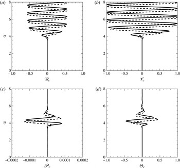
3.4 Numerical results
Composite solutions are computed for four different cases, including both incompressible and compressible (supersonic) boundary layers, with large and small values of
 $k_{1}$
.
3.4.1 Case 1: incompressible boundary layer with large
 $k_{1}$

Figure 1 shows the profile of the wall-normal velocity for
 $k_{1}=k_{2}=k_{3}=5$
and
 $E=1$
at
 $M=0$
and
 $R=400$
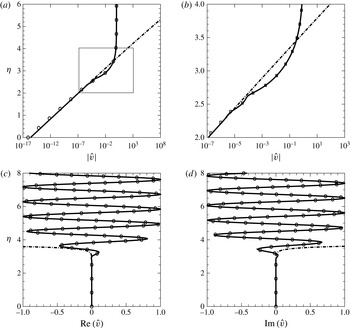
. The edge-layer solution matches smoothly with the imposed free-stream disturbance on one hand, and with the main-deck WKB solution on the other, reaffirming the basis on which the composite solution is constructed. The composite solution holds in the entire boundary layer. It turns out that the edge-layer solution and the composite solution are almost the same. The disturbance in the main boundary layer is very small, indicating that free-stream vortical disturbances are almost completely trapped in, or absorbed by, the edge layer. This is the phenomenon of ‘shear sheltering’.
The profile of the wall-normal velocity
 $v$
for
 $M=0$
,
 $R=400$
and
 $k_{1}=k_{2}=k_{3}=5$
. Panel (b) zooms into the range
 $2<{\it\eta}<4$
. Solid lines: the composite solution
 $\mathscr{V}_{c}$
; symbols: the edge-layer solution
 $\hat{v}$
; dash-dotted lines: the WKB solution in the main deck
 $v^{\dagger }$
.

The composite solutions for the velocities
 $(u,v,w)$
and the pressure
 $p$
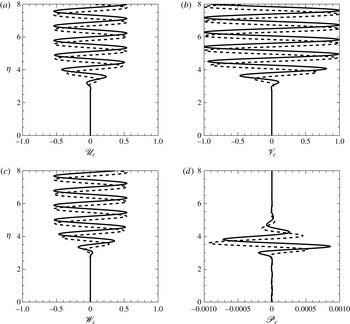
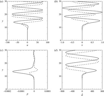
are displayed in figure 2. All three velocity components have comparable magnitudes in the edge layer. In the free stream, only a vortical disturbance is present, but within the edge layer a pressure fluctuation is generated, which decays exponentially in the free stream. These behaviours are consistent with the physical nature of the disturbance.
The composite solution
 $\mathscr{U}_{c},\mathscr{V}_{c},\mathscr{W}_{c}$
and
 $\mathscr{P}_{c}$
of an entrained disturbance with a short wavelength (
 $k_{1}=k_{2}=k_{3}=5$
) and
 $E=1$
at
 $M=0$
and
 $R=400$
. Solid lines: real parts; dashed lines: imaginary parts.

3.4.2 Case 2: incompressible boundary layer with small
$k_{1}$

Although the asymptotic solution in this paper is obtained for
 $k_{1}\gg 1$
, it is actually applicable as well to fairly small
 $k_{1}$
provided that
 $k_{1}\gg R^{-1}$
. The composition solution for
 $k_{1}=0.02$
,
 $k_{2}=k_{3}=1$
and
 $E=1$
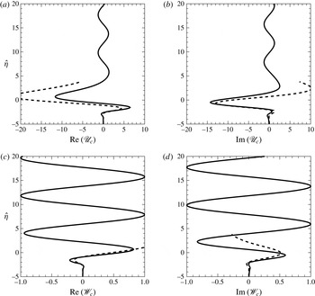
is shown in figure 3. Note that while the transverse velocities remain comparable with the disturbance level in the free stream, the streamwise velocity in the edge layer acquires an amplitude approximately 10 times as large. The amplified streamwise velocity leads to formation of streaks in the edge layer.
The composite solution for
 $\mathscr{U}_{c}$
and
 $\mathscr{W}_{c}$
of an entrained disturbance with a long streamwise wavelength (
 $k_{1}=0.02$
,
 $k_{2}=k_{3}=1$
) for
 $E=1$
,
 $M=0$
and
 $R=2000$
, and comparison with the asymptotic solution in terms of the Hankel function (Dong & Wu Reference Dong and Wu2013). Solid lines: the composite solutions; dashed lines: the Hankel function solution.

For the low-frequency case, i.e.
 $R^{-1}\ll {\it\omega}\approx k_{1}\ll 1$
, the solution can be expressed in terms of the Hankel function (Leib et al.
Reference Leib, Wundrow and Goldstein1999; Dong & Wu Reference Dong and Wu2013). A comparison with this asymptotic solution is displayed in figure 3. The composite solution and the Hankel function approximation agree reasonably well for
 $\hat{{\it\eta}}=O(1)$
, i.e. in the edge layer. The agreement deteriorates however as
 $\hat{{\it\eta}}\rightarrow \infty$
, which is expected since the solution in terms of the Hankel function is no longer valid in the free stream. The present composite solution therefore provides a better characterization of the vortical disturbance.
3.4.3 Case 3: compressible boundary layer with large
$k_{1}$

Figure 4 shows the profile of the wall-normal velocity
 $v$
for a disturbance with
 $k_{1}=k_{2}=k_{3}=5$
and
 $E=1$
at
 $M=4.5$
and
 $R=4000$
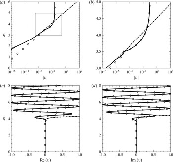
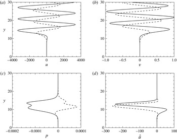
. Again, there is a smooth matching between the edge-layer and main-deck solutions at the outer reaches of the boundary layer. There is an appreciable difference between the two, but they both merge with the composite solution as expected. The composite solutions
 $\mathscr{U}_{c},\mathscr{V}_{c},\mathscr{P}_{c}$
and
 ${\it\Theta}_{c}$
are displayed in figure 5; the spanwise velocity
 $\mathscr{W}_{c}$
is not shown as it is similar to
 $\mathscr{V}_{c}$
. Only a vortical disturbance is present in the free stream, but it generates both pressure and temperature perturbations in the edge layer. The induced pressure fluctuation is fairly small, whereas the induced entropy disturbance is comparable with the vortical disturbance.
The profile of the wall-normal velocity
 $v$
for
 $k_{1}=k_{2}=k_{3}=5$
and
 $E=1$
at
 $M=4.5$
and
 $R=4000$
. Panel (b) zooms into the range
 $3<{\it\eta}<5$
. Solid lines: the composite solution
 $\mathscr{V}_{c}$
; symbols: the edge-layer solution
 $\hat{v}$
; dash-dotted lines: the WKB solution in the main deck
 $v^{\dagger }$
.

The composite solutions
 $\mathscr{U}_{c}$
,
 $\mathscr{V}_{c}$
,
 $\mathscr{P}_{c}$
and
 ${\it\Theta}_{c}$
of an entrained disturbance with a short wavelength (
 $k_{1}=k_{2}=k_{3}=5$
) and
 $E=1$
at
 $M=4.5$
and
 $R=4000$
. Solid lines: real parts, dashed lines: imaginary parts.

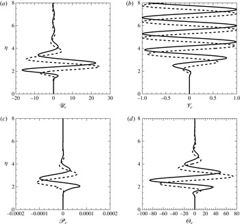
3.4.4 Case 4: compressible boundary layer with small
$k_{1}$

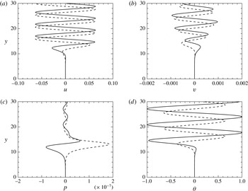
Figure 6 shows the composite solutions
 $\mathscr{U}_{c}$
,
 $\mathscr{V}_{c}$
,
 $\mathscr{P}_{c}$
and
 ${\it\Theta}_{c}$
for a disturbance with a relatively long streamwise wavelength (
 $k_{1}=0.02$
,
 $k_{2}=k_{3}=3.14$
) at
 $M=4.5$
and
 $R=4000$
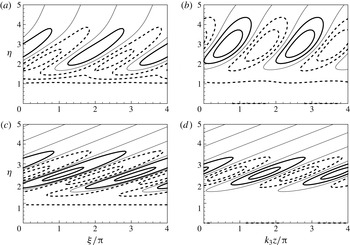
. Similar to the incompressible case, the streamwise velocity is much amplified in the edge layer, attaining a maximum amplitude approximately 20 times that of the free-stream disturbance. This implies formation of strong velocity streaks in the edge layer. Interestingly, for compressible boundary layers a free-stream vortical disturbance drives also an extremely strong temperature fluctuation in the edge layer with its amplitude being approximately 70 times that of the FSVD. Thermal streaks are therefore expected to form. As the streamwise velocity and the temperature fluctuations acquire larger magnitudes only within the edge layer, this phenomenon is entirely physically acceptable. It should not be confused with the non-physical features of ‘vortical entropy entanglement’ and ‘abnormal anisotropy’ that continuous spectra exhibit; see § 4 below.
The composite solution for
 $\mathscr{U}_{c}$
,
 $\mathscr{V}_{c}$
,
 $\mathscr{P}_{c}$
and
 ${\it\Theta}_{c}$
of an entrained disturbance with a long streamwise wavelength (
 $k_{1}=0.02$
),
 $k_{2}=k_{3}=3.14$
and
 $E=1$
at
 $M=4.5$
and
 $R=4000$
. Solid lines: real parts, dashed lines: imaginary parts.

Quantities of interest are the total spanwise vorticity
 ${\it\Omega}_{z}$
and streamwise velocity
 $u_{T}$
in the edge layer, which are given by
 $$\begin{eqnarray}\displaystyle & \displaystyle {\it\Omega}_{z}={\it\epsilon}\text{i}/(\sqrt{2}\tilde{k}^{2})[\tilde{k}_{1}(\hat{v}^{\prime \prime }-\tilde{k}^{2}\hat{v})+\tilde{k}_{3}\hat{{\it\Omega}}^{\prime }]\text{e}^{\text{i}{\it\xi}}+\text{c.c.}-\hat{a}\text{e}^{-{\it\eta}_{0}^{2}/2}\text{e}^{-\hat{{\it\eta}}}, & \displaystyle\end{eqnarray}$$
 $$\begin{eqnarray}\displaystyle & \displaystyle u_{T}={\it\epsilon}\text{i}/\tilde{k}^{2}[\tilde{k}_{1}\hat{v}^{\prime }-\tilde{k}_{3}\hat{{\it\Omega}}]\text{e}^{\text{i}{\it\xi}}+\text{c.c.}+1-\frac{\hat{a}}{\hat{{\it\eta}}-{\it\beta}}\text{e}^{-{\it\eta}_{0}^{2}/2}\text{e}^{-\hat{{\it\eta}}}, & \displaystyle\end{eqnarray}$$
where
 ${\it\epsilon}$
is the magnitude of the disturbance and
 ${\it\xi}=k_{1}x+k_{3}z-{\it\omega}t+\tilde{k}_{2}(1+{\it\delta}\hat{{\it\beta}})/{\it\delta}^{2}$
. Figure 7 displays contours of
 ${\it\Omega}_{z}$
and
 $u_{T}$
in
 $({\it\xi},{\it\eta})$
and
 $(z,{\it\eta})$
planes, respectively, for two cases of small
 $k_{1}$
, which are chosen because the spanwise vorticity and streamwise velocity of the perturbation acquire large amplitudes. Contours of
 ${\it\Omega}_{z}$
and
 $u_{T}$
illustrate the spatial structure of vortices and streaks.
Contours of the spanwise vorticity
 ${\it\Omega}_{z}$
(a,c) and the total streamwise velocity
 $u_{T}$
(b,d). Panels (a) and (b) are for
 $M=0$
,
 $R=2000$
,
 $k_{1}=0.02$
,
 $k_{2}=k_{3}=1$
and
 $E=1.0$
with
 ${\it\epsilon}=0.05$
; (c) and (d) are for
 $M=4.5$
,
 $R=4000$
,
 $k_{1}=0.02$
,
 $k_{2}=k_{3}=3.14$
and
 $E=1.0$
. The solid, dashed and thin lines in (a) and (c) represent the positive, negative and zero levels, respectively; and those in (b) and (d) represent the levels above, below and equal to 1, respectively.

4 Continuous spectra
4.1 Finite Reynolds number formulation
When the terms representing the non-parallel-flow effects are ignored at the outset, the linearized N–S equations (2.17)–(2.22) reduce to (Balakumar & Malik Reference Balakumar and Malik1992)
 $$\begin{eqnarray}\left.\begin{array}{@{}c@{}}\text{i}k_{1}u+v^{\prime }+\text{i}k_{3}w=\displaystyle -T[\text{i}(k_{1}U-{\it\omega}){\it\rho}-(T^{\prime }/T^{2})v],\\ \text{i}(k_{1}U-{\it\omega})u+U^{\prime }v=\displaystyle -\text{i}k_{1}Tp+\frac{T}{R}\left[{\rm\Delta}u+\frac{1}{3}{\it\mu}\,\text{i}k_{1}S+(U^{\prime }{\it\mu}^{\prime }T^{\prime })^{\prime }+{\it\mu}^{\prime }T^{\prime }\text{i}k_{1}v\right]\\ \text{i}(k_{1}U-{\it\omega})v=\displaystyle -Tp^{\prime }+\frac{T}{R}\left[{\rm\Delta}v+\frac{1}{3}{\it\mu}S^{\prime }+{\it\mu}^{\prime }(T^{\prime }v^{\prime }+\text{i}k_{1}U^{\prime }{\it\theta})-\frac{2}{3}{\it\mu}^{\prime }T^{\prime }S\right],\\ \text{i}(k_{1}U-{\it\omega})w=\displaystyle -\text{i}k_{3}Tp+\frac{T}{R}\left[{\rm\Delta}w+\frac{1}{3}{\it\mu}\,\text{i}k_{3}S+{\it\mu}^{\prime }T^{\prime }\text{i}k_{3}v\right],\\ \begin{array}{@{}rcl@{}}~\text{i}(k_{1}U-{\it\omega}){\it\theta}+T^{\prime }v\ & =\ & \displaystyle ({\it\gamma}-1)TM^{2}\text{i}(k_{1}U-{\it\omega})p+\frac{T}{\mathit{Pr}\,R}[{\rm\Delta}{\it\theta}+({\it\mu}^{\prime }T^{\prime }{\it\theta})^{\prime }]\\ ~\ & \ & \displaystyle +\,\frac{({\it\gamma}-1)TM^{2}}{R}[2{\it\mu}U^{\prime }(u^{\prime }+\text{i}k_{1}v)+{\it\mu}^{\prime }U^{\prime 2}{\it\theta}],\end{array}\\ T{\it\rho}+{\it\theta}/T={\it\gamma}M^{2}p,\end{array}\right\}\end{eqnarray}$$
where a prime denotes the derivative with respect to
 $y$
, except
 ${\it\mu}^{\prime }$
, which is with respect to
 $T$
. The above equations can be recast into a system of first-order equations (Joo & Durbin Reference Joo and Durbin2010, Reference Joo and Durbin2012)
 $$\begin{eqnarray}\frac{\text{d}\unicode[STIX]{x1D731}}{\text{d}y}+\unicode[STIX]{x1D63F}(y)\unicode[STIX]{x1D731}=0,\end{eqnarray}$$
where
 $\unicode[STIX]{x1D731}$
is a vector of dimension eight,
 $$\begin{eqnarray}\unicode[STIX]{x1D731}(y)=(u,u^{\prime },v,p,{\it\theta},{\it\theta}^{\prime },w,w^{\prime })^{\text{T}},\end{eqnarray}$$
and
 $\unicode[STIX]{x1D63F}$
is an
 $8\times 8$
matrix, whose expression is given in appendix B.
The system (4.2) is subject to four boundary conditions at the wall,
 $$\begin{eqnarray}u(0)=v(0)=w(0)={\it\theta}(0)=0,\end{eqnarray}$$
and four upper boundary conditions, which represent vortical, acoustic and entropy modes, as will be shown below. The resulting boundary-layer problem is to be solved by the finite-difference scheme of Malik (Reference Malik1990).
The upper boundary conditions are derived as follows. In the free stream, the gradient of the base flow vanishes so that the system (4.2) has constant coefficients, and the general solution is of the form
 $$\begin{eqnarray}\unicode[STIX]{x1D731}=\mathop{\sum }_{j=1}^{8}A_{j}\boldsymbol{b}^{(j)}\text{e}^{{\it\lambda}_{j}y},\end{eqnarray}$$
where
 ${\it\lambda}_{j}$
and
 $\boldsymbol{b}^{(j)}$
denote the eigenvalue and eigenfunction of
 $\unicode[STIX]{x1D63F}_{\infty }\equiv \lim _{y\rightarrow \infty }\unicode[STIX]{x1D63F}$
, respectively, and the constant
 $A_{j}$
represents the amplitude of the component with eigenvalue
 ${\it\lambda}_{j}$
. The eigenvalues are found to be (Balakumar & Malik Reference Balakumar and Malik1992)
 $$\begin{eqnarray}\left.\begin{array}{@{}c@{}}{\it\lambda}_{1}={\it\lambda}_{3}=-{\it\lambda}_{2}=-{\it\lambda}_{4}=\displaystyle [\text{i}(k_{1}-{\it\omega})R+k_{1}^{2}+k_{3}^{2}]^{1/2},\\ {\it\lambda}_{5}=-{\it\lambda}_{6}=\displaystyle {\textstyle \frac{1}{2}}\left[(b_{22}+b_{33})-\sqrt{(b_{22}+b_{33})^{2}+4(b_{23}b_{32}-b_{22}b_{33})}\right]^{1/2},\\ {\it\lambda}_{7}=-{\it\lambda}_{8}=\displaystyle {\textstyle \frac{1}{2}}\left[(b_{22}+b_{33})+\sqrt{(b_{22}+b_{33})^{2}+4(b_{23}b_{32}-b_{22}b_{33})}\right]^{1/2},\end{array}\right\}\end{eqnarray}$$
where
 $$\begin{eqnarray}\left.\begin{array}{@{}c@{}}\displaystyle b_{22}=k_{1}^{2}+k_{3}^{2}-R(k_{1}-{\it\omega})^{2}\frac{{\textstyle \frac{3}{4}}{\it\gamma}M^{2}-({\it\gamma}-1)\mathit{Pr}\,M^{2}}{{\textstyle \frac{3}{4}}R+\text{i}(k_{1}-{\it\omega}){\it\gamma}M^{2}},\quad b_{23}=\frac{R(k_{1}-{\it\omega})^{2}({\textstyle \frac{3}{4}}-\mathit{Pr})}{{\textstyle \frac{3}{4}}R+\text{i}(k_{1}-{\it\omega}){\it\gamma}M^{2}},\\ \displaystyle b_{32}=-\text{i}(k_{1}-{\it\omega})({\it\gamma}-1)\mathit{Pr}\,M^{2}R,\quad b_{33}=\text{i}(k_{1}-{\it\omega})\mathit{Pr}\,R+k_{1}^{2}+k_{3}^{2}.\end{array}\right\}\end{eqnarray}$$
It should be mentioned that although
 ${\it\lambda}_{1}={\it\lambda}_{3}$
and
 ${\it\lambda}_{2}={\it\lambda}_{4}$
, the corresponding eigenvectors are all different.
The nature of the eigenvalues transpires when their large Reynolds number approximation is examined. There exist three branches of continuous spectra: acoustic, entropy and vortical. The acoustic-mode branch is not the focus of the present study. As a contrast with the latter two branches, it suffices to note that an acoustic mode has the property that
 $k_{1}-{\it\omega}=O(1)$
for
 $R\gg 1$
, and represents a clear physical entity, an acoustic disturbance in the free stream. The fluctuation in the free stream consists simultaneously of the Fourier components with vertical wavenumbers
 $\pm k_{2}$
, which are coupled. Such a coupling is entirely physical with the two components representing the incident and reflected sound waves. In contrast, vortical and entropy modes do not represent any physical entity, and the coupling between
 $\pm k_{2}$
components in them is non-physical as we will show.
4.1.1 Vortical-mode branch
If
 $k_{1}-{\it\omega}=O(R^{-1})$
, which is the case for vortical and entropy disturbances, the eigenvalues simplify to:
 $$\begin{eqnarray}{\it\lambda}_{5,6}=\pm [k_{1}^{2}+k_{3}^{2}]^{1/2},\quad {\it\lambda}_{7,8}=\pm [\text{i}(k_{1}-{\it\omega})\mathit{Pr}\,R+k_{1}^{2}+k_{3}^{2}]^{1/2},\end{eqnarray}$$
in the limit
 $R\rightarrow \infty$
(and
 $M=O(1)$
), while
 ${\it\lambda}_{1,2,3,4}$
remain as given in (4.6). Setting either
 ${\it\lambda}_{1}={\it\lambda}_{3}=\text{i}k_{2}$
or
 ${\it\lambda}_{2}={\it\lambda}_{4}=-\text{i}k_{2}$
, where
 $k_{2}$
represents the wall-normal wavenumber, then we obtain
 $$\begin{eqnarray}k_{1}^{2}+k_{2}^{2}+k_{3}^{2}+\text{i}(k_{1}-{\it\omega})R=0,\end{eqnarray}$$
which is the dispersion relation for vortical modes. Their phase speeds are
 $$\begin{eqnarray}c=\frac{{\it\omega}}{k_{1}}=1+\frac{\text{i}(k_{1}^{2}+k_{2}^{2}+k_{3}^{2})}{{\it\omega}R}\rightarrow 1\quad \text{as}~R\rightarrow \infty .\end{eqnarray}$$
For spatial vortical modes, only
 $k_{1}$
is complex with a positive imaginary part of
 $O(R^{-1})$
. It follows from (4.8) that for
 $R\gg 1$
,
 $$\begin{eqnarray}{\it\lambda}_{5}=-{\it\lambda}_{6}\approx [k_{1}^{2}+k_{3}^{2}]^{1/2}=(a+b\text{i}),\end{eqnarray}$$
where
 $a$
and
 $b$
are real with
 $a>0$
, and
 $$\begin{eqnarray}{\it\lambda}_{7}=-{\it\lambda}_{8}\approx [-\mathit{Pr}\,k_{2}^{2}+(1-\mathit{Pr})(k_{1}^{2}+k_{3}^{2})]^{1/2}.\end{eqnarray}$$
Note that if
 $\mathit{Pr}=1$
, then
 ${\it\lambda}_{7}=-{\it\lambda}_{8}=\text{i}k_{2}$
, that is, they represent entropy modes. More generally for
 $\mathit{Pr}\neq 1$
,
 ${\it\lambda}_{7}$
and
 ${\it\lambda}_{8}$
are both nearly pure imaginary with real parts of
 $O(R^{-1})$
provided that
 $$\begin{eqnarray}\mathit{Pr}\,k_{2}^{2}+(\mathit{Pr}-1)({\it\omega}^{2}+k_{3}^{2})>0;\end{eqnarray}$$
the corresponding eigenvectors,
 $\boldsymbol{b}^{(7)}$
and
 $\boldsymbol{b}^{(8)}$
, represent temperature/density fluctuations persistent in the free stream (
 $0\ll y\ll R$
), and hence will be referred to as ‘quasi entropy modes’ since one of them (
 ${\it\lambda}_{8}$
say) eventually decays, while the other (
 ${\it\lambda}_{7}$
say) becomes unbounded when
 $y\gg R$
. These modes have vertical wavenumbers
 $\pm {\it\sigma}$
, with
 $$\begin{eqnarray}{\it\sigma}\approx [\mathit{Pr}\,k_{2}^{2}+(\mathit{Pr}-1)({\it\omega}^{2}+k_{3}^{2})]^{1/2}.\end{eqnarray}$$
When (4.13) is violated,
 ${\it\lambda}_{7}$
and
 ${\it\lambda}_{8}$
are complex with
 $O(1)$
positive and negative real parts, respectively. Thus regardless whether
 $\mathit{Pr}=1$
or not, we may designate
 ${\it\lambda}_{7}$
and
 ${\it\lambda}_{8}$
as having positive and negative real parts, respectively.
In the present paper, we consider the case of
 $\mathit{Pr}=0.72$
and
 $k_{1}\leqslant O(k_{2})=O(k_{3})$
, with
 ${\it\omega}$
,
 $k_{2}$
and
 $k_{3}$
being chosen such that (4.13) is always satisfied. As a result,
 ${\it\lambda}_{1}={\it\lambda}_{3}=\text{i}k_{2}$
and
 ${\it\lambda}_{2}={\it\lambda}_{3}=-\text{i}k_{2}$
are all purely imaginary, and
 ${\it\lambda}_{7,8}$
are nearly purely imaginary, whereas
 ${\it\lambda}_{5,6}$
are almost real with positive and negative real parts, respectively.
In order to keep the perturbation bounded at infinity, it is necessary to set
 $A_{5}=0$
and we also set
 $A_{7}=0$
to exclude the unbounded ‘quasi entropy mode’. There are several options for specifying the remaining parameters, one of which may be taken to be unity as a normalization condition. The solution in the free stream is in general a supposition of four branches of vortical modes and a ‘quasi entropy mode’, which can be designated according to (wall-normal wavenumber, amplitude) as
 $(k_{2},A_{1}),(-k_{2},A_{2}),(k_{2},A_{3})$
,
 $(-k_{2},A_{4})$
and
 $(-{\it\sigma},A_{8})$
. The wall-normal velocity and vorticity fluctuations,
 $v$
and
 ${\it\Omega}$
, are given by
 $$\begin{eqnarray}v=\mathop{\sum }_{j=1}^{4}A_{j}b_{3}^{(j)}\text{e}^{{\it\lambda}_{j}y},\quad {\it\Omega}=\mathop{\sum }_{j=1}^{4}A_{j}(\text{i}k_{3}b_{1}^{(j)}-\text{i}k_{1}b_{7}^{(j)})\text{e}^{{\it\lambda}_{j}y},\end{eqnarray}$$
respectively. Numerical calculations and the asymptotic analysis will show that these modes, including those with wavenumbers
 $\pm k_{2}$
, are ‘entangled’ in the sense that the ratios of their amplitudes are fixed by the presence of the boundary layer. Similar to incompressible boundary layers considered in Dong & Wu (Reference Dong and Wu2013), this feature of the continuous spectra, referred to as ‘Fourier-component entanglement’, is non-physical since the spectral composition (i.e. the amplitude ratios) should be determined by how the perturbations are generated upstream rather than by the boundary layer underneath.
For the purpose of illustration, we set
 $A_{2}=1$
, and perform calculations and present the results for three cases, all with
 $M=4.5$
and
 $R=4000$
.
(i) We set
 $A_{3}=0$
. The values of
 $A_{1,4,8}$
are determined by solving the boundary-value problem. For the given set of parameters, the amplitudes of the two other vortical modes and the induced ‘quasi entropy mode’ are found to be
 $$\begin{eqnarray}A_{1}=-0.0826+0.105\text{i},\quad A_{4}=-0.00791+0.0125\text{i},\quad A_{8}=0.847-4.627\text{i}.\end{eqnarray}$$
That
 $A_{1}$
must take a specific value signifies the entanglement of Fourier components
 $\pm k_{2}$
of the vortical disturbance. Moreover, the fact that
 $A_{8}\neq 0$
means that an entropy perturbation must also be present, whose amplitude is dictated by the vortical mode
 $(-k_{2},A_{2})$
in the free stream. This will be referred to as ‘vortical–entropy entanglement’, which occurs in compressible boundary layers. Figure 8 shows the profiles of
 $\hat{u} ,\hat{v},\hat{p}$
and
 $\hat{{\it\theta}}$
. The streamwise velocity in the free stream has a much larger amplitude than that of the transverse velocities
 $\hat{v}$
and
 ${\hat{w}}$
(not shown). This ‘abnormal anisotropy’ arises not because of conditions upstream but is due to the presence of the boundary layer. The temperature fluctuation, associated with the entangled ‘quasi entropy mode’, acquires an extraordinarily large amplitude as well in the free stream, a mathematical reason for which will be offered later. This feature, which was observed previously by Joo & Durbin (Reference Joo and Durbin2010) in their calculations, is not physically acceptable even though the ‘quasi entropy mode’ would eventually attenuate when
 $y$
is very large (
 $y\gg R$
); see later. A pressure fluctuation is induced by the vortical disturbance but is confined within the edge layer, i.e. there is no vorticity–acoustic entanglement.
The profiles of continuous modes with
 $A_{3}=A_{5}=A_{7}=0$
and
 $A_{2}=1$
in the upper boundary condition, where the eigenfunctions are normalized by
 $\max (|\hat{v}_{\infty }|)$
. The thick line marks the location of
 ${\it\delta}_{99}$
. Solid lines: real parts; dashed lines: imaginary parts. The parameters are
 $M=4.5$
,
 $R=4000$
,
 $k_{1}=0.01$
and
 $k_{2}=k_{3}=1.0$
.

(ii) We set
 $A_{1}=0$
. Then it is found that
 $$\begin{eqnarray}A_{3}=-0.00200-0.00151\text{i},\quad A_{4}=-0.0118+0.0134\text{i},\quad A_{8}=0.696-7.29\text{i}.\end{eqnarray}$$
Once again, Fourier components
 $\pm k_{2}$
of the vortical disturbance are entangled, and a ‘quasi entropy mode’
 $(-{\it\sigma},A_{8})$
is entangled with the vortical disturbance due to the presence of the boundary layer. The profiles displayed in figure 9 indicate that the streamwise velocity and the temperature in the free stream exhibit ‘abnormal anisotropy’.
The profiles of continuous modes with
 $A_{1}=A_{5}=A_{7}=0$
and
 $A_{2}=1$
in the upper boundary condition. Solid lines: real parts; dashed lines: imaginary parts. The parameters are
 $M=4.5$
,
 $R=4000$
,
 $k_{1}=0.01$
and
 $k_{2}=k_{3}=1.0$
.

(iii) We set
 $A_{8}=0$
. This is an extreme case in that any entropy disturbance is completely excluded with only velocity perturbations being present in the free stream. The vortical–entropy entanglement is thus avoided at outset. All four vortical modes, which appear in pairs with
 $\pm k_{2}$
vertical wavenumbers, must be present simultaneously. With
 $A_{2}=1$
, the amplitudes of the other three modes are calculated, and it is found that the vortical disturbance must have the composition
 $$\begin{eqnarray}(A_{1},A_{2},A_{3},A_{4})=(-0.268+0.249\text{i},1,0.00281+0.00341\text{i},-0.000766+0.0126\text{i}).\end{eqnarray}$$
The result indicates a full entanglement of Fourier components. Note that the composition (4.18) of the vortical-mode amplitudes is dictated completely by the boundary layer, and only with this specific composition does the entropy disturbance vanish in the free stream (i.e.
 $A_{7}=A_{8}=0$
). Physical vortical disturbances of course do not have such a composition in general. The profiles of
 $\hat{u} ,\hat{v},\hat{p}$
and
 $\hat{{\it\theta}}$
are displayed in figure 10. The streamwise velocity has a much larger amplitude than that of the normal velocity. Although not shown, the spanwise velocity has a very large amplitude in this case. Both the pressure and temperature perturbations are generated and remain trapped in the edge layer.
The profiles of continuous modes for the case where entropy components are absent (i.e.
 $A_{7}=A_{8}=0$
). Solid lines: real parts; dashed lines: imaginary parts. The parameters are
 $M=4.5$
,
 $R=4000$
,
 $k_{1}=0.01$
and
 $k_{2}=k_{3}=1$
.

4.1.2 Entropy-mode branch
As was already alluded to above,
 ${\it\omega}-k_{1}=O(R^{-1})$
for the entropy modes, and so the large-
 $R$
asymptotes of the eigenvalues are the same as given in (4.8). Setting
 ${\it\lambda}_{7}=-{\it\lambda}_{8}=\text{i}k_{2}$
gives the following dispersion relation for entropy modes,
 $$\begin{eqnarray}k_{1}^{2}+k_{2}^{2}+k_{3}^{2}+\text{i}(k_{1}-{\it\omega})\mathit{Pr}\,R=0,\end{eqnarray}$$
which implies that their phase speeds are given by
 $$\begin{eqnarray}c=\frac{{\it\omega}}{k_{1}}=1+\frac{\text{i}(k_{1}^{2}+k_{2}^{2}+k_{3}^{2})}{{\it\omega}\mathit{Pr}\,R}\rightarrow 1\quad \text{as}~R\rightarrow \infty .\end{eqnarray}$$
The eigenvalues
 ${\it\lambda}_{1,2,3,4}$
as given in (4.6) now simplify to
 $$\begin{eqnarray}{\it\lambda}_{1}={\it\lambda}_{3}=-{\it\lambda}_{2}=-{\it\lambda}_{4}\approx \mp \text{i}[k_{2}^{2}+(1-\mathit{Pr})(k_{1}^{2}+k_{3}^{2})]^{1/2}/\sqrt{\mathit{Pr}}.\end{eqnarray}$$
For spatial entropy modes,
 $k_{1}$
is complex with an
 $O(R^{-1})$
positive imaginary part. It follows that
 ${\it\lambda}_{1,2,3,4}$
are nearly purely imaginary with real parts being of
 $O(R^{-1})$
when
 $\mathit{Pr}<1$
(e.g.
 $\mathit{Pr}=0.72$
). The disturbances corresponding to
 ${\it\lambda}_{1,2,3,4}$
are oscillatory, and of vortical nature, in the free stream, and will be referred to as induced vortical modes. The branches are chosen such that
 $\text{Re}({\it\lambda}_{1})=\text{Re}({\it\lambda}_{3})>0$
while
 $\text{Re}({\it\lambda}_{2})=\text{Re}({\it\lambda}_{4})<0$
. On the other hand,
 $$\begin{eqnarray}{\it\lambda}_{5}=-{\it\lambda}_{6}\approx \pm [k_{1}^{2}+k_{3}^{2}]^{1/2}=\pm (a+b\text{i}),\end{eqnarray}$$
where
 $a$
and
 $b$
are real with
 $a>0$
.
The boundary-value problem for continuous entropy modes is similar to that for continuous vortical modes. It remains necessary to set
 $A_{5}=0$
. Assuming that the temperature fluctuation is specified in terms of entropy modes, we set
 $A_{8}=1$
. We now take
 $A_{1}=A_{3}=0$
in order to exclude the slowly attenuating induced vortical modes.
 $A_{2}$
,
 $A_{4}$
and
 $A_{7}$
are to be found, and the calculations give their values as
 $$\begin{eqnarray}A_{2}=-0.000896-0.00164\text{i},\quad A_{4}=0.0878+0.0225\text{i},\quad A_{7}=-0.136+0.166\text{i}.\end{eqnarray}$$
The profiles of the velocity, pressure and temperature are displayed figure 11. For the choice of
 $A_{1}=A_{3}=0$
, the Fourier entanglement between
 $\pm k_{2}$
vorticity modes is avoided, but the two Fourier components in the entropy modes are now entangled since
 $A_{7}$
is fixed by the boundary-value problem. Furthermore, there is an entropy–vorticity entanglement, that is, entropy fluctuations force the presence of vortical disturbances in the free stream as figure 11 indicates. This is not physically acceptable even though the induced vortical disturbance is rather small. The induced pressure fluctuation is confined in the edge layer, i.e. entropy–acoustic entanglement does not occur.
The profiles of continuous modes with
 $A_{8}=1$
and
 $A_{1}=A_{3}=A_{5}=0$
in the upper boundary conditions, where the eigenfunctions are normalized by
 $\max (|\hat{{\it\theta}}_{\infty }|)$
. Solid lines: real parts; dashed lines: imaginary parts. The parameters are
 $M=4.5$
,
 $R=4000$
,
 $k_{1}=0.01$
and
 $k_{2}=k_{3}=1.0$
.

In summary, vortical and entropy branches of the continuous spectra exhibit several non-physical features including Fourier-component entanglement, vortical–entropy and entropy–vortical entanglements as well as abnormal anisotropy. Among these, the vortical–entropy entanglement (coupling) and abnormally large size of the induced entropy disturbance were noted by Joo & Durbin (Reference Joo and Durbin2010). They also pointed out that these cause a problem when continuous modes are used to represent free-stream disturbances. Without recognizing the cause of these features, Joo & Durbin (Reference Joo and Durbin2010) sought to avoid them by removing certain coupling terms in the disturbance equations. However, there is no justification for this step, and the meaning of the resulting solution to the reduced system remains unclear. Furthermore, the removal of those coupling terms does not prevent the entanglement of Fourier components in the velocity and temperature perturbations. The present work indicates that all of these non-physical features are due to neglecting non-parallelism since our analysis in § 3 shows that the true entrained disturbance does not exhibit any of these features when non-parallelism is included.
4.2 The large Reynolds number asymptotic description of continuous spectra
In order to provide a contrast with the physical process of entrainment and to explain some of the numerical findings concerning the continuous spectra, the asymptotic description of continuous modes given by Dong & Wu (Reference Dong and Wu2013) for disturbances in incompressible boundary layers and with
 $O({\it\delta}^{\ast })$
wavelength, is now generalised to compressible boundary layers for the case where wavelengths are comparable with the width of the edge layer. This shorter-wavelength scaling regime turns out to be more general than that for
 $O({\it\delta}^{\ast })$
wavelengths. Analytical progress can be made for genuine boundary-layer profiles, and there is no need to use an artificial piecewise linear profile (cf. Jacobs & Durbin Reference Jacobs and Durbin1998; Zaki & Durbin Reference Zaki and Durbin2005; Zaki & Saha Reference Zaki and Saha2009).
With acoustic modes being excluded from consideration, the far-field asymptotes consist of vortical or entropy modes, leading to two branches of continuous spectra.
4.2.1 Vortical-mode branch
In this case, the wall-normal velocity
 $v$
and vorticity
 ${\it\Omega}$
are specified as
 $$\begin{eqnarray}v=A\text{e}^{-\text{i}k_{2}y}+B\text{e}^{\text{i}k_{2}y}+C\text{e}^{-\bar{k}y},\quad {\it\Omega}=E\text{e}^{-\text{i}k_{2}y}+F\text{e}^{\text{i}k_{2}y},\end{eqnarray}$$
where
 $\bar{k}$
is given by (3.4),
 $A$
,
 $B$
,
 $C$
,
 $E$
and
 $F$
are all constants, among which we can set
 $A=1$
, while
 $B$
,
 $C$
and one of
 $E$
and
 $F$
are to be determined. It is worth noting that they are related to the eigenvectors in (4.5) via the relations,
 $$\begin{eqnarray}C=A_{6}b_{3}^{(6)},\quad (B,F)^{\text{T}}=\mathscr{M}_{1}(A_{1},A_{3})^{\text{T}},\quad (A,E)^{\text{T}}=\mathscr{M}_{2}(A_{2},A_{4})^{\text{T}},\end{eqnarray}$$
where the transfer matrices are
 $$\begin{eqnarray}\displaystyle & \displaystyle \mathscr{M}_{1}=\left[\begin{array}{@{}cc@{}}b_{3}^{(1)} & b_{3}^{(3)}\\ \text{i}(k_{3}b_{1}^{(1)}-k_{1}b_{7}^{(1)}) & \text{i}(k_{3}b_{1}^{(3)}-k_{1}b_{7}^{(3)})\end{array}\right], & \displaystyle\end{eqnarray}$$
 $$\begin{eqnarray}\displaystyle & \displaystyle \mathscr{M}_{2}=\left[\begin{array}{@{}cc@{}}b_{3}^{(2)} & b_{3}^{(4)}\\ \text{i}(k_{3}b_{1}^{(2)}-k_{1}b_{7}^{(2)}) & \text{i}(k_{3}b_{1}^{(4)}-k_{1}b_{7}^{(4)})\end{array}\right]. & \displaystyle\end{eqnarray}$$
Thus if we specify
 $A$
and
 $E$
, or
 $B$
and
 $F$
, we can obtain
 $A_{1}$
and
 $A_{3}$
, or
 $A_{2}$
and
 $A_{4}$
, and vice versa.
From the momentum and energy equations, we obtain the solution for the induced pressure and temperature
 $$\begin{eqnarray}\displaystyle & \displaystyle p=-\frac{1}{\bar{k}R}(k_{1}^{2}+k_{2}^{2}+k_{3}^{2})C\text{e}^{-\bar{k}y}, & \displaystyle\end{eqnarray}$$
 $$\begin{eqnarray}\displaystyle & \displaystyle {\it\theta}=R_{1}\text{e}^{-\text{i}{\it\sigma}y}+R_{2}\text{e}^{\text{i}{\it\sigma}y}-\frac{({\it\gamma}-1)M^{2}}{\bar{k}R}(k_{1}^{2}+k_{2}^{2}+k_{3}^{2})C\text{e}^{-\bar{k}y}, & \displaystyle\end{eqnarray}$$
where
 $k_{1}$
is related to
 ${\it\omega}$
via (4.9), and
 ${\it\sigma}$
is given by (4.14). Note that the temperature fluctuation consists of terms
 $\text{e}^{\pm \text{i}{\it\sigma}y}$
, which are oscillatory when the condition (4.13) holds. As will be shown below, at least one of these two terms must be present, and they represent the ‘quasi entropy modes’ forced by the vortical disturbance, indicating that the entropy modes are dependent of the vortical modes. This is in contrast to the entrainment problem, where such terms are absent (see (3.8)) since entropy and vortical disturbances in the free stream can be independent.
In the limit
 $R\rightarrow \infty$
, eigenfunctions of the continuous modes acquire an asymptotic structure consisting of the main part of the boundary layer and a relatively thin edge layer located at the outer reach of the boundary layer. The width of the edge layer is
 ${\it\delta}\equiv {\it\eta}_{0}^{-1}\ll 1$
with
 ${\it\eta}_{0}\gg 1$
is specified by the the equation
 $$\begin{eqnarray}{\it\eta}_{0}^{3}\text{e}^{{\it\eta}_{0}^{2}/2}=2\hat{a}{\it\omega}R.\end{eqnarray}$$
The analysis presented in the earlier work by Dong & Wu (Reference Dong and Wu2013) pertains to the scaling
 $k_{2}=O(1)$
and
 $k_{3}=O(1)$
. The present work is concerned with disturbances of shorter wavelength
 $k_{2}=O({\it\delta}^{-1})$
and
 $k_{3}=O({\it\delta}^{-1})$
, for which the analysis must be modified.
The solution in the edge layer expands as
 $$\begin{eqnarray}(u,v,w,p,{\it\Omega})=(\hat{u} ,\hat{v},{\hat{w}},\hat{p}/({\it\delta}R),\hat{{\it\Omega}}/(\sqrt{2}{\it\delta})).\end{eqnarray}$$
Note that (4.30) and the form of the solution (4.31) differ from (3.9) and (3.18) respectively in that the dependence on
 $\bar{x}$
is absent. The normal velocity of a continuous mode generates a temperature/density fluctuation, and the dominant balance in the energy equation suggests that the solution for the latter can be written as
 $$\begin{eqnarray}{\it\theta}=-{\it\rho}=\text{e}^{(1/2)(1-\mathit{Pr}){\it\eta}_{0}^{2}}\hat{{\it\theta}}.\end{eqnarray}$$
Substitution of (4.31)–(4.32) into the continuity and momentum equations (2.17)–(2.20) but with non-parallelism being artificially suppressed leads to the edge-layer equations,
 $$\begin{eqnarray}\displaystyle & \displaystyle \text{i}\tilde{k}_{1}\hat{u} +\hat{v}^{\prime }+\text{i}\tilde{k}_{3}{\hat{w}}=0, & \displaystyle\end{eqnarray}$$
 $$\begin{eqnarray}\displaystyle & \displaystyle \left.\begin{array}{@{}c@{}}(\hat{\mathscr{D}}^{2}-\tilde{k}_{1}^{2}-\tilde{k}_{3}^{2})\hat{u} +\text{i}(\text{e}^{-\hat{{\it\eta}}}+{\it\omega}_{1})\hat{u} -\text{e}^{-\hat{{\it\eta}}}\hat{v}/(\tilde{{\it\omega}}\sqrt{2})=\text{i}\sqrt{2}\tilde{k}_{1}\hat{p},\\ (\hat{\mathscr{D}}^{2}-\tilde{k}_{1}^{2}-\tilde{k}_{3}^{2}){\hat{w}}+\text{i}(\text{e}^{-\hat{{\it\eta}}}+{\it\omega}_{1}){\hat{w}}=\text{i}\sqrt{2}\tilde{k}_{3}\hat{p},\end{array}\right\} & \displaystyle\end{eqnarray}$$
 $$\begin{eqnarray}\displaystyle & \displaystyle [(\hat{\mathscr{D}}^{2}-\tilde{k}_{1}^{2}-\tilde{k}_{3}^{2})\hat{v}+\text{i}(\text{e}^{-\hat{{\it\eta}}}+{\it\omega}_{1})\hat{v}]=\sqrt{2}\hat{p}_{\hat{{\it\eta}}}. & \displaystyle\end{eqnarray}$$
They are similar to (3.21) and (3.22), but the crucial difference is that the first-order derivatives,
 $\hat{u} ^{\prime }$
,
 ${\hat{w}}^{\prime }$
and
 $\hat{v}^{\prime }$
, as well as terms with coefficient
 $\text{i}k_{2}$
, in the three momentum equations are now absent. Eliminating
 $\hat{u}$
and
 ${\hat{w}}$
among (4.33)–(4.35), we obtain
 $$\begin{eqnarray}\displaystyle & \displaystyle [(\mathscr{D}^{2}+\tilde{k}_{2}^{2}+\text{i}\text{e}^{-\hat{{\it\eta}}})(\mathscr{D}^{2}-\tilde{k}_{1}^{2}-\tilde{k}_{3}^{2})-\text{i}\text{e}^{-\hat{{\it\eta}}}]\hat{v}=0, & \displaystyle\end{eqnarray}$$
 $$\begin{eqnarray}\displaystyle & \displaystyle (\mathscr{D}^{2}+\tilde{k}_{2}^{2}+\text{i}\text{e}^{-\hat{{\it\eta}}})\hat{{\it\Omega}}=\text{i}\tilde{k}_{3}/(\sqrt{2}\tilde{{\it\omega}})\text{e}^{-\hat{{\it\eta}}}\hat{v}. & \displaystyle\end{eqnarray}$$
The boundary conditions for (4.36) and (4.37) are
 $$\begin{eqnarray}\displaystyle & \displaystyle \left.\begin{array}{@{}c@{}}\hat{v}\rightarrow \displaystyle \hat{A}\text{e}^{-\text{i}\tilde{k}_{2}\hat{{\it\eta}}}+\hat{B}\text{e}^{\text{i}\tilde{k}_{2}\hat{{\it\eta}}}+{\hat{C}}\text{e}^{-\tilde{k}\hat{{\it\eta}}}\quad \text{as}~\hat{{\it\eta}}\rightarrow \infty ,\\ \hat{v}\rightarrow \displaystyle 0,\quad \hat{v}^{\prime }\rightarrow 0\quad \text{as}~\hat{{\it\eta}}\rightarrow -\infty ;\end{array}\right\} & \displaystyle\end{eqnarray}$$
 $$\begin{eqnarray}\displaystyle & \displaystyle \hat{{\it\Omega}}\rightarrow \hat{E}\text{e}^{-\text{i}\tilde{k}_{2}\hat{{\it\eta}}}+\hat{F}\text{e}^{\text{i}\tilde{k}_{2}\hat{{\it\eta}}}\quad \text{as}~\hat{{\it\eta}}\rightarrow \infty ,\quad \hat{{\it\Omega}}\rightarrow 0\quad \text{as}~\hat{{\it\eta}}\rightarrow -\infty , & \displaystyle\end{eqnarray}$$
where
 $$\begin{eqnarray}\displaystyle & \displaystyle (\hat{A},\hat{B},{\hat{C}})=(A\text{e}^{-\text{i}\tilde{k}_{2}(1+{\it\delta}\hat{{\it\beta}})/{\it\delta}^{2}},\,B\text{e}^{\text{i}\tilde{k}_{2}(1+{\it\delta}\hat{{\it\beta}})/{\it\delta}^{2}},\,C\text{e}^{-\tilde{k}_{2}(1+{\it\delta}\hat{{\it\beta}})/{\it\delta}^{2}}), & \displaystyle\end{eqnarray}$$
 $$\begin{eqnarray}\displaystyle & \displaystyle (\hat{E},\hat{F})=(\sqrt{2}{\it\delta}E\text{e}^{-\text{i}\tilde{k}_{2}(1+{\it\delta}\hat{{\it\beta}})/{\it\delta}^{2}},\,\sqrt{2}{\it\delta}F\text{e}^{\text{i}\tilde{k}_{2}(1+{\it\delta}\hat{{\it\beta}})/{\it\delta}^{2}}). & \displaystyle\end{eqnarray}$$
The WKB solution in the main layer consists of the inviscid and viscous parts. The former turns out to be essentially the same as that for entrained disturbances, while the latter remains the same as for
 $k_{2}=O(1)$
and
 $k_{3}=O(1)$
considered in Dong & Wu (Reference Dong and Wu2013). Omitting the details, we find that matching with the edge-layer solution requires that as
 $\hat{{\it\eta}}\rightarrow -\infty$
,
 $$\begin{eqnarray}\displaystyle & \displaystyle \hat{v}\rightarrow b_{0}\text{e}^{(1+\tilde{k}^{2})^{1/2}\hat{{\it\eta}}}+c_{0}\text{e}^{5\hat{{\it\eta}}/4}\exp \{-2\text{e}^{-{\rm\pi}\text{i}/4}\text{e}^{-\hat{{\it\eta}}/2}\}, & \displaystyle\end{eqnarray}$$
 $$\begin{eqnarray}\displaystyle \hat{{\it\Omega}} & \rightarrow & \displaystyle (\tilde{k}_{3}/(\sqrt{2}\tilde{{\it\omega}}))b_{0}\text{e}^{[(1+\tilde{k}^{2})^{1/2}-1]\hat{{\it\eta}}}\nonumber\\ \displaystyle & & \displaystyle +\left\{d_{0}\left[1+\left(\frac{3}{16}-\tilde{k}_{2}^{2}\right)\text{e}^{{\rm\pi}\text{i}/4}\text{e}^{\hat{{\it\eta}}/2}\right]-\frac{\tilde{k}_{3}c_{0}}{\sqrt{2}\tilde{{\it\omega}}}\text{e}^{-\text{i}{\rm\pi}/4}\text{e}^{\hat{{\it\eta}}/2}\right\}\text{e}^{\hat{{\it\eta}}/4}\exp (-2\text{e}^{-\text{i}{\rm\pi}/4}\text{e}^{-\hat{{\it\eta}}/2}).\nonumber\\ \displaystyle & & \displaystyle\end{eqnarray}$$
The above asymptotic behaviours provide more precise boundary conditions than (4.38) and (4.39) for
 $\hat{v}$
and
 $\hat{{\it\Omega}}$
respectively, and they can alternatively be derived by considering the balances in equations (4.36) and (4.37) in the limit
 $\hat{{\it\eta}}\rightarrow -\infty$
.
Substitution of (4.31) and (4.32) into the energy equation in (4.1) shows that
 $\hat{{\it\theta}}$
satisfies the equation
 $$\begin{eqnarray}\mathit{Pr}^{-1}(\hat{\mathscr{D}}^{2}-\tilde{k}_{1}^{2}-\tilde{k}_{3}^{2})\hat{{\it\theta}}+\text{i}(\text{e}^{-\hat{{\it\eta}}}+{\it\omega}_{1})\hat{{\it\theta}}=\mathit{Pr}\,\hat{b}/(\hat{a}\tilde{{\it\omega}}\sqrt{2})\text{e}^{-\mathit{Pr}\,\hat{{\it\eta}}}\hat{v}.\end{eqnarray}$$
The boundary condition consistent with the equation is
 $$\begin{eqnarray}\hat{{\it\theta}}\rightarrow \hat{R}_{1}\text{e}^{-\text{i}\tilde{{\it\sigma}}\hat{{\it\eta}}}+\hat{R}_{2}\text{e}^{\text{i}\tilde{{\it\sigma}}\hat{{\it\eta}}}\quad \text{as}~\hat{{\it\eta}}\rightarrow \infty ;\quad \hat{{\it\theta}}\rightarrow 0\quad \text{as}~\hat{{\it\eta}}\rightarrow -\infty ,\end{eqnarray}$$
where
 $$\begin{eqnarray}(\hat{R}_{1},\hat{R}_{2})=\text{e}^{-(1/2)(1-\mathit{Pr}){\it\eta}_{0}^{2}}(R_{1}\text{e}^{-\text{i}\tilde{k}_{2}(1+{\it\delta}\hat{{\it\beta}})/{\it\delta}^{2}},R_{2}\text{e}^{\text{i}\tilde{k}_{2}(1+{\it\delta}\hat{{\it\beta}})/{\it\delta}^{2}}),\end{eqnarray}$$
and
 $$\begin{eqnarray}\tilde{{\it\sigma}}=[\mathit{Pr}\,\tilde{k}_{2}^{2}+(\mathit{Pr}-1)(\tilde{{\it\omega}}^{2}+\tilde{k}_{3}^{2})]^{1/2}.\end{eqnarray}$$
When
 $[(\mathit{Pr}-1)(\tilde{{\it\omega}}^{2}+\tilde{k}_{3}^{2})+\mathit{Pr}\,\tilde{k}_{2}^{2}]>0$
, which is always the case for
 $\mathit{Pr}\geqslant 1$
,
 $\tilde{{\it\sigma}}$
is purely imaginary, but
 $(\hat{R}_{1},\hat{R}_{2})\neq (0,0)$
in general as we will show.
In the limit
 $R\rightarrow \infty$
, the system governing the continuous spectra becomes only partially coupled: the equations for the normal vorticity
 $\hat{{\it\Omega}}$
and the temperature
 $\hat{{\it\theta}}$
are coupled only to that for the normal velocity
 $\hat{v}$
, whilst the latter is independent. The solutions for
 $\hat{v}$
,
 $\hat{{\it\Omega}}$
and
 $\hat{{\it\theta}}$
can be obtained in sequence.
The boundary-value problem (4.37) with (4.39) corresponds to (C 1) of appendix C with
 ${\it\sigma}=\tilde{k}_{2}$
,
 ${\it\kappa}=1$
and
 $f=\text{i}\tilde{k}_{3}/(\sqrt{2}\tilde{{\it\omega}})\hat{v}$
. Inserting these into the general results (C 8) and (C 3) with (C 5), we obtain the relation between
 $\hat{E}$
and
 $\hat{F}$
,
 $$\begin{eqnarray}\hat{E}-\frac{|{\it\Gamma}(2\text{i}\tilde{k}_{2})|^{2}}{{\it\Gamma}^{2}(2\text{i}\tilde{k}_{2})}\text{e}^{\tilde{k}_{2}{\rm\pi}}\hat{F}=-\frac{{\rm\pi}\text{i}\tilde{k}_{3}/(\sqrt{2}\tilde{{\it\omega}})\text{e}^{-\tilde{k}_{2}{\rm\pi}/2}}{2\tilde{k}_{2}{\it\Gamma}(2\text{i}\tilde{k}_{2})}\int _{-\infty }^{\infty }\text{e}^{-\hat{{\it\eta}}}H_{{\it\nu}}^{(1)}({\it\zeta})\hat{v}\,\text{d}\hat{{\it\eta}},\end{eqnarray}$$
and the solution for
 $\hat{{\it\Omega}}$
,
 $$\begin{eqnarray}\hat{{\it\Omega}}=\frac{{\rm\pi}\text{i}\tilde{k}_{3}/(\sqrt{2}\tilde{{\it\omega}})}{2\sinh (2\tilde{k}_{2}{\rm\pi})}\int _{0}^{{\it\zeta}}\tilde{{\it\zeta}}[\text{J}_{-{\it\nu}}({\it\zeta})\text{J}_{{\it\nu}}(\tilde{{\it\zeta}})-\text{J}_{{\it\nu}}({\it\zeta})\text{J}_{-{\it\nu}}(\tilde{{\it\zeta}})]\hat{v}\,\text{d}\tilde{{\it\zeta}}+d_{0}^{+}\text{J}_{{\it\nu}}({\it\zeta})+d_{0}^{-}\text{J}_{-{\it\nu}}({\it\zeta}),\end{eqnarray}$$
where
 ${\it\nu}=2\text{i}\tilde{k}_{2}$
and
 $$\begin{eqnarray}d_{0}^{+}={\it\Gamma}(1+2\text{i}\tilde{k}_{2})\text{e}^{\tilde{k}_{2}{\rm\pi}/2}\hat{E},\quad d_{0}^{-}={\it\Gamma}(1-2\text{i}\tilde{k}_{2})\text{e}^{-\tilde{k}_{2}{\rm\pi}/2}\hat{F}.\end{eqnarray}$$
The constraint (4.48) implies that the amplitudes of the Fourier components
 $\text{e}^{\pm \text{i}k_{2}y}$
in the normal vorticity are interrelated rather than being independent.
The boundary-value problem (4.44)–(4.45) corresponds to (C 1) with
 ${\it\kappa}=\mathit{Pr}$
,
 ${\it\sigma}=\tilde{{\it\sigma}}$
and
 $f=\hat{b}/(\hat{a}\tilde{{\it\omega}}\sqrt{2})\text{e}^{-(\mathit{Pr}-1)\hat{{\it\eta}}}\hat{v}$
. The general result (C 3) with (C 5) is specialized to this case to give the solution for
 $\hat{{\it\theta}}$
,
 $$\begin{eqnarray}\hat{{\it\theta}}=-\frac{{\rm\pi}\hat{b}/(\hat{a}\tilde{{\it\omega}}\sqrt{2})}{2\sinh (2{\it\sigma}{\rm\pi})}\int _{0}^{{\it\zeta}}\tilde{{\it\zeta}}[J_{-\tilde{{\it\nu}}}({\it\zeta})J_{\tilde{{\it\nu}}}(\tilde{{\it\zeta}})-J_{\tilde{{\it\nu}}}({\it\zeta})J_{-\tilde{{\it\nu}}}(\tilde{{\it\zeta}})]\text{e}^{-(\mathit{Pr}-1)\hat{{\it\eta}}}\hat{v}\,\text{d}\tilde{{\it\zeta}}+s_{0}^{+}J_{\tilde{{\it\nu}}}({\it\zeta})+s_{0}^{-}J_{-\tilde{{\it\nu}}}({\it\zeta}),\end{eqnarray}$$
where
 $\tilde{{\it\nu}}=2\text{i}\tilde{{\it\sigma}}$
,
 ${\it\zeta}=2(\text{i}\mathit{Pr})^{1/2}\text{e}^{-\hat{{\it\eta}}/2}$
and
 $$\begin{eqnarray}s_{0}^{+}={\it\Gamma}(1+2\text{i}\tilde{{\it\sigma}})\text{e}^{\tilde{{\it\sigma}}{\rm\pi}/2}\mathit{Pr}^{-\text{i}\tilde{{\it\sigma}}}\hat{R}_{1},\quad s_{0}^{-}={\it\Gamma}(1-2\text{i}\tilde{{\it\sigma}})\text{e}^{-\tilde{{\it\sigma}}{\rm\pi}/2}\mathit{Pr}^{\text{i}\tilde{{\it\sigma}}}\hat{R}_{2}.\end{eqnarray}$$
The relation,
 $$\begin{eqnarray}\hat{R}_{1}-\frac{|{\it\Gamma}(2\text{i}\tilde{{\it\sigma}})|^{2}}{{\it\Gamma}^{2}(2\text{i}\tilde{{\it\sigma}})}\mathit{Pr}^{2\text{i}\tilde{{\it\sigma}}}\text{e}^{\tilde{{\it\sigma}}{\rm\pi}}\hat{R}_{2}=-\frac{{\rm\pi}\mathit{Pr}^{\text{i}\tilde{{\it\sigma}}+1}\text{e}^{-\tilde{{\it\sigma}}{\rm\pi}/2}}{2\tilde{{\it\sigma}}{\it\Gamma}(2\text{i}\tilde{{\it\sigma}})}\hat{b}/(\hat{a}\tilde{{\it\omega}}\sqrt{2})\int _{-\infty }^{\infty }\text{e}^{-\mathit{Pr}\,\hat{{\it\eta}}}H_{\tilde{{\it\nu}}}^{(1)}({\it\zeta})\,\hat{v}\,\text{d}\hat{{\it\eta}},\end{eqnarray}$$
between
 $\hat{R}_{1}$
and
 $\hat{R}_{2}$
follows from (C 8). Provided that the right-hand side does not vanish, at least one of
 $\hat{R}_{1}$
and
 $\hat{R}_{2}$
must be non-zero, indicating that in the free stream, entropy fluctuations of large amplitude must simultaneously be present along with vortical fluctuations when (4.13) holds. The asymptotic analysis confirms the entanglement of entropy and vortical modes found earlier by finite Reynolds number calculations. Note that the entanglements are caused by neglecting the non-parallel-flow effect; when the latter is included in the analysis of the entrainment, there is no such an entanglement (cf. § 3). If it is insisted that
 $\hat{R}_{1}=\hat{R}_{2}=0$
(as was the case in the calculation displayed in figure 10), then it is required that
 $$\begin{eqnarray}\int _{-\infty }^{\infty }\text{e}^{-\mathit{Pr}\,\hat{{\it\eta}}}H_{\tilde{{\it\nu}}}^{(1)}({\it\zeta})\,\hat{v}\,\text{d}\hat{{\it\eta}}=0,\end{eqnarray}$$
which can be satisfied only if the amplitudes of the four vortical modes obey a specific composition such as (4.18).
By solving (4.36) subject to the boundary conditions (4.38) and (4.42), we can determine
 $\hat{B}$
and
 ${\hat{C}}$
. The result for two-dimensional disturbances in the incompressible limit is shown in figure 12, and a comparison is made with the prediction by solving the O–S equation as well as with the analytical approximation of Dong & Wu (Reference Dong and Wu2013), which holds only when
 $k_{2}=O(1)$
. Despite a moderate value of
 $R$
, the two asymptotic theories both give reasonably accurate predictions for
 $k_{2}=O(1)$
. For large
 $k_{2}$
, only the present asymptotic approach based on the short-wavelength scaling is able to give the result in agreement with the O–S solution.
Comparison of the coefficients
 $B$
and
 $C$
for
 $M=0$
,
 $R=580$
,
 ${\it\omega}=0.179$
and
 $k_{3}=0$
. Dashed lines: asymptotic prediction by Dong & Wu (Reference Dong and Wu2013); dash-dotted lines: asymptotic prediction in the present paper; solid lines: numerical solution of the O–S equation.

Comparison of the asymptotic and finite Reynolds number predictions for
 $\hat{B}$
,
 $\hat{F}$
and
 $\hat{R}_{1}$
, where
 $R=4000$
,
 $M=4.5$
and
 $k_{1}=k_{3}=3.14$
. (a,c,e) Real part; (b,d,f) imaginary part. Solid lines: finite-
 $R$
solution; dashed lines (with or without symbols): asymptotic prediction.

We solved also the boundary-value problem (4.36) with (4.38) and (4.42) for three-dimensional disturbances in a supersonic boundary layer at Mach number
 $M=4.5$
. The resulting
 $\hat{B}$
is shown in figure 13 and compared with that obtained by the finite Reynolds number calculation. Subsequently, the boundary-value problems, (4.37) with (4.39) for the vorticity and (4.44)–(4.45) for the temperature, are solved for
 $E=0$
and
 $R_{2}=0$
respectively, to obtain
 $\hat{F}$
and
 $\hat{R}_{1}$
. Their values are found to be the same as those given by formulae (4.48) and (4.53) as expected, confirming that the latter are correct. As figure 13 indicates, there is a fair agreement between the asymptotic and finite Reynolds number predictions.
4.2.2 Entropy-mode branch
We analyse briefly the entropy-mode branch, for which the temperature fluctuation has the far-field asymptote,
 $$\begin{eqnarray}{\it\theta}=r_{1}\text{e}^{-\text{i}k_{2}y}+r_{2}\text{e}^{\text{i}k_{2}y},\end{eqnarray}$$
where
 $k_{j}$
(
 $j=1,2,3$
) and
 ${\it\omega}$
satisfy the dispersion relation (4.19).
The temperature fluctuation drives velocity fluctuations through the continuity equation. The dominant balance shows that the solution in the edge layer takes the form
 $$\begin{eqnarray}(u,v,w,p,{\it\Omega})={\it\delta}\text{e}^{-{\it\eta}_{0}^{2}/2}(\hat{u} ,\hat{v},{\hat{w}},\hat{p}/({\it\delta}R),\hat{{\it\Omega}}/(\sqrt{2}{\it\delta})).\end{eqnarray}$$
Since the velocity is very small, the energy equation is decoupled from it and reduces to
 $$\begin{eqnarray}\mathit{Pr}^{-1}(\mathscr{D}^{2}+\tilde{k}_{2}^{2}){\it\theta}+\text{i}\text{e}^{-\hat{{\it\eta}}}{\it\theta}=0,\end{eqnarray}$$
and the boundary conditions are found to be
 $$\begin{eqnarray}{\it\theta}\rightarrow \hat{r}_{1}\text{e}^{-\text{i}\tilde{k}_{2}\hat{{\it\eta}}}+\hat{r}_{2}\text{e}^{\text{i}\tilde{k}_{2}\hat{{\it\eta}}}\quad \text{as}~\hat{{\it\eta}}\rightarrow \infty ,\quad {\it\theta}\rightarrow 0\quad \text{as}~\hat{{\it\eta}}\rightarrow -\infty ,\end{eqnarray}$$
where
 $(\hat{r}_{1},\hat{r}_{2})=(r_{1}\text{e}^{-\text{i}\tilde{k}_{2}(1+{\it\delta}\hat{{\it\beta}})/{\it\delta}^{2}},r_{2}\text{e}^{\text{i}\tilde{k}_{2}(1+{\it\delta}\hat{{\it\beta}})/{\it\delta}^{2}})$
, obtained by rewriting (4.55) in terms of the edge-layer variable
 $\hat{{\it\eta}}$
and matching with (4.58). The boundary-value problem (4.57) with (4.58) is a homogeneous version (
 $f\equiv 0$
) of (C 1) with
 ${\it\sigma}=\tilde{k}_{2}$
and
 ${\it\kappa}=\mathit{Pr}$
. Specializing the general results (C 9) and (C 10) to the present situation yields
 $$\begin{eqnarray}\displaystyle & \displaystyle \hat{r}_{1}/\hat{r}_{2}=\frac{|{\it\Gamma}(2\text{i}\tilde{k}_{2})|^{2}}{{\it\Gamma}^{2}(2\text{i}\tilde{k}_{2})}\mathit{Pr}^{2\text{i}\tilde{k}_{2}}\text{e}^{\tilde{k}_{2}{\rm\pi}}, & \displaystyle\end{eqnarray}$$
 $$\begin{eqnarray}\displaystyle & \displaystyle {\it\theta}=\frac{\text{i}{\rm\pi}}{{\it\Gamma}(2\text{i}\tilde{k}_{2})}\text{e}^{-\tilde{k}_{2}{\rm\pi}/2}\mathit{Pr}^{\text{i}\tilde{k}_{2}}\hat{r}_{2}H_{{\it\nu}}^{(1)}({\it\zeta}), & \displaystyle\end{eqnarray}$$
where
 ${\it\nu}=2\text{i}\tilde{k}_{2}$
and
 ${\it\zeta}=2(\text{i}\mathit{Pr})^{1/2}\text{e}^{-\hat{{\it\eta}}/2}$
. The relation (4.59) implies that the Fourier components
 $\text{e}^{\pm \text{i}k_{2}y}$
of the entropy mode are entangled. As
 $\hat{{\it\eta}}\rightarrow -\infty$
,
 $$\begin{eqnarray}{\it\theta}\rightarrow \frac{\sqrt{{\rm\pi}}}{{\it\Gamma}(2\text{i}\tilde{k}_{2})}\text{e}^{\tilde{k}_{2}{\rm\pi}/2+{\rm\pi}\text{i}/8}\mathit{Pr}^{\text{i}\tilde{k}_{2}-1/4}\hat{r}_{2}\text{e}^{\hat{{\it\eta}}/4}\exp \{-2\sqrt{\mathit{Pr}}\text{e}^{-{\rm\pi}\text{i}/4}\text{e}^{-{\it\eta}/2}\}.\end{eqnarray}$$
The continuity equation becomes
 $$\begin{eqnarray}\text{i}\tilde{k}_{1}\hat{u} +\hat{v}^{\prime }+\text{i}\tilde{k}_{3}{\hat{w}}=-\text{i}\tilde{k}_{1}\text{e}^{-\hat{{\it\eta}}}\hat{{\it\theta}},\end{eqnarray}$$
while the momentum equations remain the same as in (4.34). From (4.34) and (4.62) it follows that
 $\hat{v}$
satisfies the inhomogeneous equation
 $$\begin{eqnarray}[(\mathscr{D}^{2}+\hat{{\it\sigma}}^{2}+\text{i}\text{e}^{-\hat{{\it\eta}}})(\mathscr{D}^{2}-\tilde{k}_{1}^{2}-\tilde{k}_{3}^{2})-\text{i}\text{e}^{-\hat{{\it\eta}}}]\hat{v}=-\text{i}\tilde{k}_{1}\text{e}^{-\hat{{\it\eta}}}F_{{\it\theta}},\end{eqnarray}$$
with
 $\hat{{\it\sigma}}$
and the forcing term
 $F_{{\it\theta}}$
given by
 $$\begin{eqnarray}\displaystyle \hat{{\it\sigma}}=[\tilde{k}_{2}^{2}+(1-\mathit{Pr})(\tilde{{\it\omega}}^{2}+\tilde{k}_{3}^{2})]^{1/2}/\sqrt{\mathit{Pr}}. & & \displaystyle\end{eqnarray}$$
 $$\begin{eqnarray}\displaystyle F_{{\it\theta}} & = & \displaystyle \{3+(1-\mathit{Pr})[(\tilde{k}_{1}^{2}+\tilde{k}_{2}^{2}+\tilde{k}_{3}^{2})/\mathit{Pr}+\text{i}\text{e}^{-\hat{{\it\eta}}}]\}{\it\theta}^{\prime }\nonumber\\ \displaystyle & & \displaystyle +\,\{-1+2\tilde{k}_{2}^{2}-(1-\mathit{Pr})(\tilde{k}_{1}^{2}+\tilde{k}_{2}^{2}+\tilde{k}_{3}^{2})/\mathit{Pr}+2(2\mathit{Pr}-1)\text{i}\text{e}^{-\hat{{\it\eta}}}\}{\it\theta},\end{eqnarray}$$
while the equation for
 $\hat{{\it\Omega}}$
reads
 $$\begin{eqnarray}(\mathscr{D}^{2}+\hat{{\it\sigma}}^{2}+\text{i}\text{e}^{-\hat{{\it\eta}}})\hat{{\it\Omega}}=\text{i}\tilde{k}_{3}/(\sqrt{2}\tilde{{\it\omega}})\text{e}^{-\hat{{\it\eta}}}\hat{v}.\end{eqnarray}$$
At the outer reach of the edge layer, the induced vortical disturbance behaves as
 $$\begin{eqnarray}\hat{v}\rightarrow \hat{A}\text{e}^{-\text{i}\hat{{\it\sigma}}\hat{{\it\eta}}}+\hat{B}\text{e}^{\text{i}\hat{{\it\sigma}}\hat{{\it\eta}}}+\cdots \,,\quad \hat{{\it\Omega}}\rightarrow \hat{E}\text{e}^{-\text{i}\hat{{\it\sigma}}\hat{{\it\eta}}}+\hat{F}\text{e}^{\text{i}\hat{{\it\sigma}}\hat{{\it\eta}}}\quad \text{as}~\hat{{\it\eta}}\rightarrow \infty .\end{eqnarray}$$
In general,
 $\hat{A}$
,
 $\hat{B}$
,
 $\hat{E}$
and
 $\hat{F}$
are non-zero, indicating that an entropy mode induces vortical disturbances in the free stream, just like a vortical mode generates entropy disturbances. This may be referred to as entropy–vorticity entanglement. Again
 $\hat{A}$
and
 $\hat{B}$
, and therefore
 $\hat{E}$
and
 $\hat{F}$
, are related, with the latter satisfying the constraint
 $$\begin{eqnarray}\hat{E}-\frac{|{\it\Gamma}(2\text{i}\hat{{\it\sigma}})|^{2}}{{\it\Gamma}^{2}(2\text{i}\hat{{\it\sigma}})}\text{e}^{\hat{{\it\sigma}}{\rm\pi}}\hat{F}=-\frac{{\rm\pi}\text{i}\tilde{k}_{3}/(\sqrt{2}\tilde{{\it\omega}})\text{e}^{-\tilde{{\it\sigma}}{\rm\pi}/2}}{2\tilde{{\it\sigma}}{\it\Gamma}(2\text{i}\tilde{{\it\sigma}})}\int _{-\infty }^{\infty }\text{e}^{-\hat{{\it\eta}}}H_{2\text{i}\hat{{\it\sigma}}}^{(1)}({\it\zeta})\,\hat{v}\,\text{d}\hat{{\it\eta}}.\end{eqnarray}$$
The asymptotic boundary-value problem (4.57) with (4.58) is solved numerically for
 $r_{1}=1$
to obtain
 $\hat{r}_{2}$
, which should be the same as the result given by the analytical expression (4.59). On the other hand, the finite Reynolds number system is solved for
 $A_{8}=1$
(equivalent to
 $r_{1}=1$
) and
 $A_{1}=A_{3}=0$
. The results are compared in figure 14. A fairly good agreement is observed, confirming the Fourier entanglement of the entropy mode. We also performed the calculation for
 $A_{2}=A_{4}=0$
, and found practically the same
 $\hat{r}_{2}$
as we did for the case of
 $A_{1}=A_{3}=0$
, consistent with the asymptotic result (4.59), which implies that
 $\hat{r}_{2}$
is independent of the choice of
 $A_{1,2,3,4}$
provided their values are sufficiently small (see (4.56)). Velocity fluctuations are induced in the free stream, indicating that the entropy–vortical entanglement occurs as is implied by the relation (4.68).
Comparison of
 $\hat{r}_{2}$
as obtained by finite-
 $R$
calculation (solid lines), large-
 $R$
asymptotic calculation (dashed lines) and (4.59) (symbols), where
 $R=4000$
,
 $M=4.5$
and
 $k_{1}=k_{3}=3.14$
. (a) Real part; (b) imaginary part.

The analysis in this section shows that in the high Reynolds number limit (
 $R\gg 1$
) the system governing the continuous spectra simplifies and becomes partially coupled. Barring the parallel-flow approximation already inherent in the continuous spectrum formulation, the present analysis is self-consistent. This asymptotically reduced system is quite different from those obtained by Joo & Durbin (Reference Joo and Durbin2010) through ad hoc approximations. All of the non-physical features of the continuous vortical and entropy modes persist in the limit
 $R\gg 1$
. The striking difference between the solutions in §§ 3 and 4.2 indicates that the continuous modes and the entrainment of vortical disturbances are fundamentally different, and associating the former with latter is incorrect.
Although the edge layers in the entrainment problem and in the continuous-mode analysis both prevent the disturbance from entering the boundary layer, there is a crucial difference: the former acts as a ‘wave absorber’, whereas the latter acts as a (spurious) ‘wave reflector’ to produce one of the entangled Fourier components in the free stream.
5 Summary and conclusions
In this paper, we have investigated the entrainment process of free-stream vortical disturbances into incompressible and compressible boundary layers. Starting from the linearized N–S equations and adopting a large Reynolds number asymptotic approach, a systematic analysis was performed for disturbances with short wavelengths on the scale of the edge-layer width, which is smaller than the local boundary-layer thickness. Non-parallelism is found to play a leading-order role in this short-wavelength regime. The resulting equations turns out to be more general than those for the case where the wavelengths comparable with the boundary-layer thickness. Appropriate asymptotic solutions in the main and edge layers are obtained, from which a composite solution is constructed. Interestingly, the solutions remain valid for long wavelengths provided that the latter are smaller than the distance to the leading edge. For relatively low-frequency disturbances, the streamwise velocity acquires a very large amplitude in the edge layer, suggesting that low- and high-speed streaks would appear. In compressible boundary layers, strong temperature fluctuations are also induced in the edge layer when the Prandtl number
 $\mathit{Pr}<1$
, leading to the formation of thermal streaks, but the temperature disturbances are rather small when
 $\mathit{Pr}>1$
.
As a contrast with the entrainment process, we have also studied continuous modes of the N–S equations linearized about a parallel mean flow, which reduce to the O–S/Squire equations in the incompressible case. Finite Reynolds number calculations indicate that vortical and entropy branches of continuous spectra exhibit several non-physical features. In addition to the known abnormal anisotropy and entanglement between Fourier components, entanglement of vortical and entropy modes occurs for compressible boundary layers, that is, a vortical mode necessarily generates an entropy disturbance in the free stream, and vice versa. The induced entropy disturbance may have a much larger amplitude than that of the driving vortical mode. A high Reynolds number analysis of continuous spectra was carried out to give explicit relations between the amplitudes of the entangled components. All these non-physical features are found to result from the neglect of non-parallelism, and none of them arises in the physical process of entrainment.
The following conclusions can be drawn from the present study and that of Dong & Wu (Reference Dong and Wu2013). Viewed individually, a continuous mode with a single frequency does not represent a true physical vortical or entropy disturbance with the same frequency despite the fact that the former satisfies the dispersion relation of the latter. The eigenfunction of a continuous vortical or entropy mode does not represent the distribution of the disturbance entrained into the boundary layer, or ‘shear sheltering’ of a free-stream disturbance. Vortical and entropy modes are therefore purely mathematical objects without any physical meaning. Owing to the constraints imposed by the entanglements, general free-stream turbulence cannot possibly be represented by a superposition of such continuous modes.
Continuous modes or their supposition have been used to specify the disturbance at the inlet of computational domain for DNS of bypass transition and receptivity processes. This popular approach was based upon the premise that the inlet disturbance introduced in this way represents the perturbation that has entered the boundary layer upstream of, or at, the computational inlet. The results of the present paper and of Dong & Wu (Reference Dong and Wu2013) prove that premise false, and the use of continuous vortical and entropy modes to specify inlet conditions is therefore inappropriate. An adequate but computationally costly approach is to extend the computational domain such that its inlet is located sufficiently far upstream of the leading edge. Appropriate vortical disturbances can then be specified at the inlet since the background flow there is almost uniform. This approach has been taken by Ovchinnikov, Piomelli & Choudhari (Reference Ovchinnikov, Piomelli and Choudhari2006), Nagarajan, Lele & Ferziger (Reference Nagarajan, Lele and Ferziger2007) for simulations of bypass transition and by Schrader et al. (Reference Schrader, Brandt, Mavriplis and Henningson2010) for simulation of receptivity to vortical disturbances.
DNS of bypass transition and receptivity in a computational domain starting from a position downstream of the leading edge can be performed with the aid of the theoretical results of Leib et al. (Reference Leib, Wundrow and Goldstein1999) and the present work. The former pertain to disturbances with frequencies
 ${\it\omega}=O(R^{-1})$
, while the latter to
 ${\it\omega}\gg 1$
, but both are valid for disturbances with
 ${\it\omega}=O(1)$
. In view of this overlapping validity, appropriate inlet conditions, representing perturbations induced by a broadband of free-stream disturbance or turbulence, can be specified as follows. For components with frequencies
 ${\it\omega}$
below a certain value
 ${\it\omega}_{c}=O(1)$
including
 ${\it\omega}=O(R^{-1})$
, the boundary-region equation approach can be used, namely the initial boundary-value problem, as described in Leib et al. (Reference Leib, Wundrow and Goldstein1999), is solved by marching to the inlet position. For components with frequencies
 ${\it\omega}>{\it\omega}_{c}$
, the composite solution constructed in this paper can be used. The inlet disturbances specified in this manner are suited for numerical simulations of bypass transition and boundary-layer receptivity to free-stream vortical disturbances in plate configurations in a computational domain excluding the leading edge. It would be interesting to simulate bypass transition using the inlet disturbances as described above, and compare the resulting transition scenarios with the previous simulations where continuous modes were used as the inlet condition.
The velocity and thermal streaks appearing in the edge layer are of interest. Their significance depends on the spectral composition of the free-stream disturbance. If the latter consists of significant portion of components with very low frequencies of
 $O(R^{-1})$
, then the resulting dominant streaks reside in the main bulk of the boundary layer. However, if significant energy is distributed in the frequency band
 $R^{-1}\ll {\it\omega}\ll 1$
, then streaks may dominate the edge layer, and once acquiring a certain threshold they may induce secondary instability in that region. Edge-layer streaks have not received much attention. The present theoretical work may stimulate further investigations. Finally, we note that Deguchi & Hall (Reference Deguchi and Hall2015) have recently shown that the edge layer can support self-sustained nonlinear free-stream coherent structures, which have the same length/time scales as those of the disturbances considered in the present work. These structures appear in the form of nonlinear eigensolutions to the N–S equations, and thus represent the intrinsic dynamics of the flow. An interesting question is how these structures are affected by, or interact with, the external (i.e. free-stream) disturbances of the same length/time scales. The analysis in the present paper may be extended to address this issue.
Acknowledgements
The authors would like to thank Professors A. I. Ruban and P. Hall (Imperial College London) for helpful discussions, and the referees for their valuable suggestions. This work was supported by the NSFC (grants 11172204, 11332007 and 11472189) and by Ministry of Education of China (doctoral grant 201220032110009).
Appendix A. The solution for the second terms in (3.70)
Substituting (3.47) into (2.17)–(2.21), we find, at higher orders, that the second terms in the expansion (3.70) are governed by equations
 $$\begin{eqnarray}\displaystyle & \displaystyle \left.\begin{array}{@{}c@{}}\text{i}\tilde{k}_{1}\bar{u}_{1}/\sqrt{2}+{\it\delta}({\it\Theta}_{0}^{\prime }/T)\bar{v}_{1}+\text{i}\tilde{k}_{3}\bar{w}_{1}/\sqrt{2}=0,\\ {\it\Theta}_{0}^{\prime }\mathscr{L}_{M}\bar{u}_{1}=\{[{\it\mu}T(\tilde{k}_{1}^{2}+\tilde{k}_{3}^{2})-\text{i}({\it\omega}_{1}+\tilde{k}_{2})U]\bar{u}_{0}-{\it\delta}^{2}(K\bar{u}_{0}^{\prime \prime }+F\bar{u}_{0}^{\prime })\}/\sqrt{2}+{\it\delta}U^{\prime }/(\tilde{{\it\omega}}T)\bar{v}_{1},\\ {\it\Theta}_{0}^{\prime }\mathscr{L}_{M}\bar{w}_{1}=\{[{\it\mu}T(\tilde{k}_{1}^{2}+\tilde{k}_{3}^{2})-\text{i}({\it\omega}_{1}+\tilde{k}_{2})U]\bar{w}_{0}-{\it\delta}^{2}(K\bar{w}_{0}^{\prime \prime }+F\bar{w}_{0}^{\prime })\}/\sqrt{2},\end{array}\right\} & \displaystyle \nonumber\\ \displaystyle & & \displaystyle\end{eqnarray}$$
 $$\begin{eqnarray}\displaystyle & \displaystyle {\it\Theta}_{0}^{\prime }\mathscr{L}_{M}\bar{v}_{1}=\sqrt{2}{\it\Theta}_{0}^{\prime }\bar{p}_{1}. & \displaystyle\end{eqnarray}$$
Eliminating
 $\bar{u}_{1}$
and
 $\bar{w}_{1}$
in (A 1), we obtain the equations for
 $\bar{v}_{1}$
and
 $\bar{{\it\Omega}}_{1}$
,
 $$\begin{eqnarray}\displaystyle & \displaystyle ({\it\Theta}_{0}^{\prime 2}/T)[K(2\bar{v}_{1}^{\prime }+(3{\it\Theta}_{0}^{\prime \prime }/{\it\Theta}_{0}^{\prime }-2T^{\prime }/T)\bar{v}_{1})+{\it\Phi}\,\bar{v}_{1}]+\text{i}(U^{\prime }/T)\bar{v}_{1}=0, & \displaystyle\end{eqnarray}$$
 $$\begin{eqnarray}\displaystyle {\it\Theta}_{0}^{\prime }\mathscr{L}_{M}\bar{{\it\Omega}}_{1} & = & \displaystyle \{[{\it\mu}T(\tilde{k}_{1}^{2}+\tilde{k}_{3}^{2})-\text{i}({\it\omega}_{1}+\tilde{k}_{2})U]\bar{{\it\Omega}}_{0}-{\it\delta}^{2}(K\bar{{\it\Omega}}_{0}^{\prime \prime }+F\bar{{\it\Omega}}_{0}^{\prime })\}/\sqrt{2}\nonumber\\ \displaystyle & & \displaystyle +\,{\it\delta}(\text{i}\tilde{k}_{3}/\tilde{{\it\omega}})(U^{\prime }/T)\bar{v}_{1},\end{eqnarray}$$
where the
 $O({\it\delta})$
and
 $O({\it\delta}^{2})$
terms are retained in order to avoid further expansion.
Solving equation (A 3), we find that
 $$\begin{eqnarray}\bar{v}_{1}=c^{-}({\it\mu}/T)^{3/4}T(1-U)^{-5/4}(U^{\prime })^{1/2}\text{e}^{H({\it\eta})},\end{eqnarray}$$
where
 $c^{-}$
is a constant to be determined. As
 ${\it\eta}\rightarrow \infty$
,
 $$\begin{eqnarray}\bar{v}_{1}\rightarrow c^{-}\hat{a}^{-3/4}({\it\eta}-{\it\beta})^{1/4}\text{e}^{3({\it\eta}-{\it\beta})^{2}/8+H_{\infty }},\end{eqnarray}$$
and so matching
 ${\it\delta}^{-2}({\it\omega}R)^{-3/4}\bar{v}_{1}$
with the edge-layer solution (3.28) determines
 $$\begin{eqnarray}c^{-}=2^{-3/4}\text{e}^{-H_{\infty }}c_{0}.\end{eqnarray}$$
Inserting (3.74) and (A 5) into (A 4), and solving the resulting equation, we obtain
 $$\begin{eqnarray}\displaystyle \bar{{\it\Omega}}_{1} & = & \displaystyle ({\it\mu}/T)^{1/4}(1-U)^{-1/4}(U^{\prime })^{1/2}\text{e}^{H({\it\eta})}\left\{\vphantom{\displaystyle \left\{\left[\frac{U^{\prime \prime }}{1-U}\right]\right\}}d_{1}-{\it\delta}c^{-}(-\text{i})^{1/2}(\tilde{k}_{3}/\tilde{{\it\omega}})(1-U)^{-1/2}\right.\nonumber\\ \displaystyle & & \displaystyle +\,\frac{\text{e}^{{\rm\pi}\text{i}/4}d}{2\sqrt{2}}\left\{\vphantom{\displaystyle \left[\frac{U^{\prime \prime }}{1-U}\right]}(\tilde{k}_{1}^{2}+\tilde{k}_{3}^{2})\int _{0}^{{\it\eta}}T^{2}({\it\mu}/T)^{1/2}(1-U)^{-1/2}\,\text{d}{\it\eta}\right.\nonumber\\ \displaystyle & & \displaystyle -\,\text{i}({\it\omega}_{1}+\tilde{k}_{2})\int _{0}^{{\it\eta}}({\it\mu}/T)^{-1/2}U(1-U)^{-1/2}\,\text{d}{\it\eta}\nonumber\\ \displaystyle & & \displaystyle -\,{\it\delta}^{2}\int _{0}^{{\it\eta}}({\it\mu}/T)^{1/2}(1-U)^{-1/2}\left[\frac{5}{16}\frac{U^{\prime 2}}{(1-U)^{2}}+\frac{1}{2}\frac{U^{\prime \prime }}{1-U}-\frac{1}{4}\left(\frac{U^{\prime \prime }}{U^{\prime }}\right)^{2}+\frac{1}{2}\frac{U^{\prime \prime \prime }}{U^{\prime }}\right]\text{d}{\it\eta}\nonumber\\ \displaystyle & & \displaystyle -\left.\!\left.{\it\delta}^{2}\int _{0}^{{\it\eta}}({\it\mu}/T)^{-1/2}(1-U)^{-1/2}F\left[\frac{1}{4}\frac{U^{\prime }}{1-U}+\frac{1}{2}\frac{U^{\prime \prime }}{U^{\prime }}\right]\text{d}{\it\eta}\right\}\right\},\end{eqnarray}$$
where
 $d_{1}$
is a constant. The reader is reminded that we have ignored those
 $O({\it\delta}^{2})$
terms which do not affect the matching. As
 ${\it\eta}\rightarrow \infty$
,
 $$\begin{eqnarray}\displaystyle \bar{{\it\Omega}}_{1} & \rightarrow & \displaystyle \hat{a}^{-1/4}({\it\eta}-{\it\beta})^{-3/4}\text{e}^{({\it\eta}-{\it\beta})^{2}/8+H_{\infty }}\left\{\vphantom{\displaystyle \frac{\text{e}^{{\it\pi}\text{i}/4}}{\sqrt{2}}}-{\it\delta}\,c^{-}(-\text{i})^{1/2}(\tilde{k}_{3}/\tilde{{\it\omega}})({\it\eta}-{\it\beta})^{1/2}\right.\nonumber\\ \displaystyle & & \displaystyle +\left.\frac{\text{e}^{{\rm\pi}\text{i}/4}d}{\sqrt{2}}\left[\tilde{k}_{1}^{2}+\tilde{k}_{3}^{2}-\text{i}({\it\omega}_{1}+\tilde{k}_{2})+\frac{3}{16}{\it\delta}^{2}({\it\eta}-{\it\beta})^{2}\right]({\it\eta}-{\it\beta})^{-1/2}\right\};\end{eqnarray}$$
here we have, as is required by matching with the edge-layer solution (3.39), taken
 $$\begin{eqnarray}\displaystyle d_{1} & = & \displaystyle -\frac{\text{e}^{{\rm\pi}\text{i}/4}d}{2\sqrt{2}}{\it\delta}^{-1}\left\{\vphantom{\left[\int _{0}^{{\it\eta}_{\infty }}\right]}(\tilde{k}_{1}^{2}+\tilde{k}_{3}^{2})\int _{0}^{\infty }[T^{2}({\it\mu}/T)^{1/2}(1-U)^{-1/2}-\mathscr{U}_{D}^{-1/2}]\,\text{d}{\it\eta}\right.\nonumber\\ \displaystyle & & \displaystyle -\,\text{i}({\it\omega}_{1}+\tilde{k}_{2})\int _{0}^{\infty }[({\it\mu}/T)^{-1/2}U(1-U)^{-1/2}-\mathscr{U}_{D}^{-1/2}]\,\text{d}{\it\eta}\nonumber\\ \displaystyle & & \displaystyle -\left.(\tilde{k}_{2}^{2}+\text{i}\tilde{k}_{2})\left[\int _{0}^{{\it\eta}_{\infty }}\mathscr{U}_{D}^{-1/2}\,\text{d}{\it\eta}-2\hat{a}^{-1/2}({\it\eta}_{\infty }-{\it\beta})^{-1/2}\text{e}^{({\it\eta}_{\infty }-{\it\beta})^{2}/2}\right]\right\},\end{eqnarray}$$
where
 $\mathscr{U}_{D}$
is given by (2.15a,b
) and
 ${\it\eta}_{\infty }>{\it\beta}$
is an arbitrary constant. Note that although the
 $O({\it\delta}^{2})$
terms in (A 8) are smaller than other terms for
 ${\it\eta}=O(1)$
, it contributes the
 ${\it\delta}^{2}({\it\eta}-{\it\beta})^{2}$
term in (A 9), which becomes of
 $O(1)$
when
 ${\it\eta}=O({\it\eta}_{d})$
, affecting the matching with the edge-layer solution (3.39). Specifically, with
 $c^{-}$
and
 $d$
given by (A 7) and (3.78) respectively, the first term in (A 9) matches, on accounting for the prefactor
 $({\it\omega}R)^{-1/4}{\it\delta}^{-2}$
, the term with coefficient
 $c_{0}$
in (3.39), whereas the second term in (A 9) matches with the second of the terms with coefficient
 $d_{0}$
in (3.39) in view of (3.34).
The streamwise and spanwise velocities can be expressed in terms of
 $\bar{v}_{1}$
and
 $\bar{{\it\Omega}}_{1}$
as
 $$\begin{eqnarray}\bar{u}_{1}=\text{i}[\sqrt{2}\tilde{k}_{1}{\it\delta}({\it\Theta}_{0}^{\prime }/T)\bar{v}_{1}-\tilde{k}_{3}\bar{{\it\Omega}}_{1}]/\tilde{k}^{2},\quad \bar{w}_{1}=\text{i}[\sqrt{2}\tilde{k}_{3}{\it\delta}({\it\Theta}_{0}^{\prime }/T)\bar{v}_{1}+\tilde{k}_{1}\bar{{\it\Omega}}_{1}]/\tilde{k}^{2}.\end{eqnarray}$$
From (A 2), the pressure is found as
 $$\begin{eqnarray}\bar{p}_{1}=\sqrt{2}c^{-}K({\it\mu}/T)^{3/4}(1-U)^{-5/4}(U^{\prime })^{1/2}\text{e}^{H}\left[\frac{U^{\prime }}{1-U}+\frac{T^{\prime }}{T}+\frac{K^{\prime }T^{\prime }}{2K}\right].\end{eqnarray}$$
As
 ${\it\eta}\rightarrow \infty$
,
 $$\begin{eqnarray}\bar{p}_{1}\rightarrow \sqrt{2}c^{-}\hat{a}^{-3/4}({\it\eta}-{\it\beta})^{5/4}\text{e}^{3({\it\eta}-{\it\beta})^{2}/8+H_{\infty }}.\end{eqnarray}$$
In view of (A 7),
 $\bar{p}_{1}$
matches to the term with coefficient
 $c_{0}$
in the edge-layer solution (3.31) as expected.
Appendix B. The matrix in the first-order system (4.2)
The non-zero elements of coefficient matrix
 $\unicode[STIX]{x1D63F}(y)$
in (4.2) are (Malik Reference Malik1990)
 $$\begin{eqnarray}\displaystyle & \displaystyle d_{12}=1; & \displaystyle\end{eqnarray}$$
 $$\begin{eqnarray}\displaystyle & \displaystyle d_{21}=\text{i}{\it\xi}R/({\it\mu}T)+k_{1}^{2}+k_{3}^{2},\quad d_{22}=-{\it\mu}^{\prime }T^{\prime }/{\it\mu}, & \displaystyle\end{eqnarray}$$
 $$\begin{eqnarray}\displaystyle & \displaystyle d_{23}=U^{\prime }R/({\it\mu}T)-\text{i}k_{1}(l_{1}T^{\prime }/T+{\it\mu}^{\prime }T^{\prime }/{\it\mu}),\quad d_{24}=\text{i}k_{1}R/{\it\mu}-k_{1}l_{1}{\it\gamma}M^{2}{\it\xi}, & \displaystyle\end{eqnarray}$$
 $$\begin{eqnarray}\displaystyle & \displaystyle d_{25}=-T^{\prime }U^{\prime \prime }/{\it\mu}-{\it\mu}^{\prime \prime }T^{\prime }U^{\prime }/{\it\mu}+k_{1}l_{1}{\it\xi}/T,\quad d_{26}=-{\it\mu}^{\prime }U^{\prime }/{\it\mu}; & \displaystyle\end{eqnarray}$$
 $$\begin{eqnarray}\displaystyle & \displaystyle d_{31}=-\text{i}k_{1},\quad d_{33}=T^{\prime }/T,\quad d_{34}=-\text{i}{\it\gamma}M^{2}{\it\xi},\quad d_{35}=\text{i}{\it\xi}/T,\quad d_{37}=-\text{i}k_{3};\qquad & \displaystyle\end{eqnarray}$$
 $$\begin{eqnarray}\displaystyle & \displaystyle d_{41}=-\text{i}{\it\chi}l_{2}k_{1}T^{\prime }/T-2\text{i}{\it\chi}k_{1}{\it\mu}^{\prime }T^{\prime }/{\it\mu},\quad d_{42}=-\text{i}{\it\chi}k_{1}, & \displaystyle\end{eqnarray}$$
 $$\begin{eqnarray}\displaystyle & \displaystyle d_{43}=-{\it\chi}[\text{i}{\it\xi}R/({\it\mu}T)+k_{1}^{2}+k_{3}^{2}]+l_{2}{\it\chi}[{\it\mu}^{\prime }T^{\prime 2}/({\it\mu}T)+T^{\prime \prime }/T], & \displaystyle\end{eqnarray}$$
 $$\begin{eqnarray}\displaystyle & \displaystyle d_{44}=-\text{i}{\it\chi}{\it\gamma}M^{2}l_{2}[{\it\xi}({\it\mu}^{\prime }T^{\prime }/{\it\mu}+T^{\prime }/T)+k_{1}U^{\prime }], & \displaystyle\end{eqnarray}$$
 $$\begin{eqnarray}\displaystyle & \displaystyle d_{45}=\text{i}{\it\chi}[k_{1}U^{\prime }(l_{2}/T+{\it\mu}^{\prime }/{\it\mu})+{\it\xi}l_{2}{\it\mu}^{\prime }T^{\prime }/({\it\mu}T)], & \displaystyle\end{eqnarray}$$
 $$\begin{eqnarray}\displaystyle & \displaystyle d_{46}=\text{i}l_{2}{\it\chi}{\it\xi}/T,\quad d_{47}=-\text{i}k_{3}{\it\chi}(2{\it\mu}^{\prime }T^{\prime }/{\it\mu}+l_{2}T^{\prime }/T),\quad d_{48}=-\text{i}k_{3}{\it\chi};\qquad & \displaystyle\end{eqnarray}$$
 $$\begin{eqnarray}\displaystyle & \displaystyle d_{56}=1; & \displaystyle\end{eqnarray}$$
 $$\begin{eqnarray}\displaystyle & \displaystyle d_{62}=-2({\it\gamma}-1)M^{2}\mathit{Pr}\,U^{\prime },\quad d_{63}=-2\text{i}({\it\gamma}-1)M^{2}\mathit{Pr}\,k_{1}U^{\prime }+\mathit{Pr}\,RT^{\prime }/({\it\mu}T),\qquad \quad & \displaystyle\end{eqnarray}$$
 $$\begin{eqnarray}\displaystyle & \displaystyle d_{64}=-\text{i}{\it\xi}({\it\gamma}-1)M^{2}\mathit{Pr}\,R/{\it\mu}, & \displaystyle\end{eqnarray}$$
 $$\begin{eqnarray}\displaystyle & \displaystyle d_{65}=\text{i}{\it\xi}R\mathit{Pr}/({\it\mu}T)+k_{1}^{2}+k_{3}^{2}-({\it\gamma}-1)M^{2}\mathit{Pr}\,{\it\mu}^{\prime }U^{\prime 2}/{\it\mu}-({\it\mu}^{\prime }T^{\prime })^{\prime }/{\it\mu},\quad d_{66}=-2{\it\mu}^{\prime }T^{\prime }/{\it\mu}; & \displaystyle \nonumber\\ \displaystyle & & \displaystyle\end{eqnarray}$$
 $$\begin{eqnarray}\displaystyle & \displaystyle d_{78}=1;\quad & \displaystyle\end{eqnarray}$$
 $$\begin{eqnarray}\displaystyle & \displaystyle d_{83}=-\text{i}k_{3}{\it\mu}^{\prime }T^{\prime }/{\it\mu}-\text{i}k_{3}l_{1}T^{\prime }/T,\quad d_{84}=\text{i}k_{3}R/{\it\mu}-k_{3}l_{1}{\it\gamma}M^{2}{\it\xi}, & \displaystyle\end{eqnarray}$$
 $$\begin{eqnarray}\displaystyle & \displaystyle d_{85}=k_{3}l_{1}{\it\xi}/T,\quad d_{87}=\text{i}{\it\xi}R/({\it\mu}T)+k_{1}^{2}+k_{3}^{2},\quad d_{88}=-{\it\mu}^{\prime }T^{\prime }/{\it\mu}, & \displaystyle\end{eqnarray}$$
where we have put
 ${\it\xi}=k_{1}U-{\it\omega}$
,
 ${\it\chi}=1/(R/{\it\mu}+\text{i}{\it\gamma}M^{2}{\it\xi}l_{2})$
and
 $l_{j}=j-2/3$
(
 $j=1,2$
).
Appendix C. The boundary-value problem arising in the analysis of continuous spectra
In the high Reynolds number analysis of continuous modes, we encounter boundary-value problems of the form,
 $$\begin{eqnarray}\left.\begin{array}{@{}c@{}}{\it\kappa}^{-1}(\hat{\mathscr{D}}^{2}+{\it\sigma}^{2}){\it\phi}+\text{i}\text{e}^{-\hat{{\it\eta}}}{\it\phi}=\text{e}^{-\hat{{\it\eta}}}f,\\ {\it\phi}\rightarrow r^{-}\text{e}^{-\text{i}{\it\sigma}\hat{{\it\eta}}}+r^{+}\text{e}^{\text{i}{\it\sigma}\hat{{\it\eta}}}\quad \text{as}~\hat{{\it\eta}}\rightarrow \infty ;\\ {\it\phi}\rightarrow 0\quad \text{as}~\hat{{\it\eta}}\rightarrow -\infty ,\end{array}\right\}\end{eqnarray}$$
for the dependent variable
 ${\it\phi}$
, which may stand for the normal vorticity
 $\hat{{\it\Omega}}$
or the temperature
 $\hat{{\it\theta}}$
in the main text. The parameters
 ${\it\kappa}$
and
 ${\it\sigma}$
take different values depending on the problems considered, and
 $f$
is a function of
 $\hat{{\it\eta}}$
representing the forcing and is allowed to be arbitrary in this appendix provided that
 $f$
and
 $\text{e}^{-\hat{{\it\eta}}/2}f$
decay sufficiently fast respectively in the limits of
 $\hat{{\it\eta}}\rightarrow -\infty$
and
 $\hat{{\it\eta}}\rightarrow \infty$
.
The differential equation in (C 1) can be written as a Bessel equation of order-
 ${\it\nu}$
in terms of the new independent variable
 ${\it\zeta}$
, where
 $$\begin{eqnarray}{\it\nu}=2\text{i}{\it\sigma},\quad {\it\zeta}=2(\text{i}{\it\kappa})^{1/2}\text{e}^{-\hat{{\it\eta}}/2}.\end{eqnarray}$$
The general solution for
 ${\it\phi}$
can therefore be expressed in terms of the first-kind Bessel functions
 $\text{J}_{\pm {\it\nu}}({\it\zeta})$
, that is,
 $$\begin{eqnarray}{\it\phi}=-\frac{(-\text{i}){\rm\pi}}{2\sin ({\it\nu}{\rm\pi})}\int _{0}^{{\it\zeta}}\tilde{{\it\zeta}}[\text{J}_{-{\it\nu}}({\it\zeta})\text{J}_{{\it\nu}}(\tilde{{\it\zeta}})-\text{J}_{{\it\nu}}({\it\zeta})\text{J}_{-{\it\nu}}(\tilde{{\it\zeta}})]f(\tilde{{\it\zeta}})\,\text{d}\tilde{{\it\zeta}}+s_{0}^{+}\text{J}_{{\it\nu}}({\it\zeta})+s_{0}^{-}\text{J}_{-{\it\nu}}({\it\zeta}),\end{eqnarray}$$
where
 $s_{0}^{\pm }$
are arbitrary constants, and use has been made of identities (9.1.15) and (9.1.27) on pages 360 and 361 of Abramowitz & Stegun (Reference Abramowitz and Stegun1964) (which will hereafter be referred to as AS). The reader is reminded that the notations used in this appendix are, unless stated otherwise, independent of those appearing in the main text.
By using the small-
 ${\it\zeta}$
asymptotes of
 $J_{\pm {\it\nu}}({\it\zeta})$
((9.1.7) on page 360 of AS), it is found that
 $$\begin{eqnarray}{\it\phi}\rightarrow \frac{s_{0}^{+}}{{\it\Gamma}(1+2\text{i}{\it\sigma})}\text{e}^{-{\it\sigma}{\rm\pi}/2}{\it\kappa}^{\text{i}{\it\sigma}}\text{e}^{-\text{i}{\it\sigma}\hat{{\it\eta}}}+\frac{s_{0}^{-}}{{\it\Gamma}(1-2\text{i}{\it\sigma})}\text{e}^{{\it\sigma}{\rm\pi}/2}{\it\kappa}^{-\text{i}{\it\sigma}}\text{e}^{\text{i}{\it\sigma}\hat{{\it\eta}}}\quad \text{as}~\hat{{\it\eta}}\rightarrow \infty ,\end{eqnarray}$$
where
 ${\it\Gamma}(\cdot )$
denotes the gamma function. Matching requires that
 $$\begin{eqnarray}s_{0}^{+}={\it\Gamma}(1+2\text{i}{\it\sigma})\text{e}^{{\it\sigma}{\rm\pi}/2}{\it\kappa}^{-\text{i}{\it\sigma}}r^{-},\quad s_{0}^{-}={\it\Gamma}(1-2\text{i}{\it\sigma})\text{e}^{-{\it\sigma}{\rm\pi}/2}{\it\kappa}^{\text{i}{\it\sigma}}r^{+}.\end{eqnarray}$$
On the other hand, using the large-
 ${\it\zeta}$
asymptotes of
 $J_{\pm {\it\nu}}$
, (9.2.1) on page 364 of AS, we find that as
 $\hat{{\it\eta}}\rightarrow -\infty$
,
 $$\begin{eqnarray}\displaystyle {\it\theta} & \rightarrow & \displaystyle \frac{\text{e}^{-{\rm\pi}\text{i}/8}}{\sqrt{{\rm\pi}}{\it\kappa}^{1/4}}\text{e}^{\hat{{\it\eta}}/4}\left\{\left[s_{0}^{+}\text{e}^{{\it\sigma}{\rm\pi}}+s_{0}^{-}\text{e}^{-{\it\sigma}{\rm\pi}}-\frac{1}{2}\text{e}^{{\it\sigma}{\rm\pi}}\int _{0}^{\infty }{\it\zeta}H_{{\it\nu}}^{(2)}({\it\zeta})f({\it\zeta})\,\text{d}{\it\zeta}\right]\text{e}^{\text{i}({\it\zeta}-{\rm\pi}/4)}\right.\nonumber\\ \displaystyle & & \displaystyle +\left.\!\left[(s_{0}^{+}\text{e}^{-{\it\sigma}{\rm\pi}}+s_{0}^{-}\text{e}^{{\it\sigma}{\rm\pi}})+\frac{1}{2}\text{e}^{-{\it\sigma}{\rm\pi}}\int _{0}^{\infty }{\it\zeta}H_{{\it\nu}}^{(1)}({\it\zeta})f({\it\zeta})\,\text{d}{\it\zeta}\right]\text{e}^{-\text{i}({\it\zeta}-{\rm\pi}/4)}\right\},\end{eqnarray}$$
where use has been made of (9.1.3) and (9.1.4) of AS, and
 $H_{{\it\nu}}^{(1)}$
and
 $H_{{\it\nu}}^{(2)}$
denote Hankel functions. For the solution to remain bounded in the limit of
 $\hat{{\it\eta}}\rightarrow -\infty$
as required in (C 1), it is necessary to set the coefficient of
 $\text{e}^{-\text{i}({\it\zeta}-{\rm\pi}/4)}$
to zero, from which and (C 5) it follows that
 $$\begin{eqnarray}r^{-}+\frac{{\it\Gamma}(1-2\text{i}{\it\sigma})}{{\it\Gamma}(1+2\text{i}{\it\sigma})}{\it\kappa}^{2\text{i}{\it\sigma}}\text{e}^{{\it\sigma}{\rm\pi}}r^{+}=-\frac{{\rm\pi}\text{i}{\it\kappa}^{\text{i}{\it\sigma}+1}\text{e}^{-{\it\sigma}{\rm\pi}/2}}{{\it\Gamma}(1+2\text{i}{\it\sigma})}\int _{-\infty }^{\infty }\text{e}^{-\hat{{\it\eta}}}H_{{\it\nu}}^{(1)}({\it\zeta})f\,\text{d}\hat{{\it\eta}}.\end{eqnarray}$$
After making use of (6.1.29) on page 256 of AS, the above relation simplifies to
 $$\begin{eqnarray}r^{-}-\frac{|{\it\Gamma}(2\text{i}{\it\sigma})|^{2}}{{\it\Gamma}^{2}(2\text{i}{\it\sigma})}{\it\kappa}^{2\text{i}{\it\sigma}}\text{e}^{{\it\sigma}{\rm\pi}}r^{+}=-\frac{{\rm\pi}{\it\kappa}^{\text{i}{\it\sigma}+1}\text{e}^{-{\it\sigma}{\rm\pi}/2}}{2{\it\sigma}{\it\Gamma}(2\text{i}{\it\sigma})}\int _{-\infty }^{\infty }\text{e}^{-\hat{{\it\eta}}}H_{{\it\nu}}^{(1)}({\it\zeta})f\,\text{d}\hat{{\it\eta}}.\end{eqnarray}$$
For a homogeneous problem,
 $f=0$
, then
 $$\begin{eqnarray}{\it\chi}\equiv r^{-}/r_{+}=\frac{|{\it\Gamma}(2\text{i}{\it\sigma})|^{2}}{{\it\Gamma}^{2}(2\text{i}{\it\sigma})}{\it\kappa}^{2\text{i}{\it\sigma}}\text{e}^{{\it\sigma}{\rm\pi}},\end{eqnarray}$$
and with
 $r^{+}$
being set to unity the complementary solution is obtained as
 $$\begin{eqnarray}{\it\phi}_{c}=\frac{\text{i}{\rm\pi}}{{\it\Gamma}(2\text{i}{\it\sigma})}\text{e}^{-{\it\sigma}{\rm\pi}/2}{\it\kappa}^{\text{i}{\it\sigma}}H_{{\it\nu}}^{(1)}({\it\zeta}).\end{eqnarray}$$
Equations (C 3) with (C 5) and (C 8)–(C 10) are the main results of this appendix, and they are used repeatedly in the main text.