1 Introduction
Steady streaming is a wave-induced residual flow driven by Reynolds stresses and balanced by viscous stresses in the Stokes boundary layer (Batchelor Reference Batchelor2000; Riley Reference Riley2001). The momentum of the streaming flow in the boundary layer can be transferred into the liquid bulk through fluid viscosity to form an Eulerian mean circulation. Streaming circulations play essential roles in fluid mass and passive scalar transport in many environments, such as inside blood vessels, cochleae and the boundary layer over ocean sediments (Lesser & Berkley Reference Lesser and Berkley1972; Schneck & Walburn Reference Schneck and Walburn1976; Holmedal & Myrhaug Reference Holmedal and Myrhaug2009). In recent years, the residual motion driven by surface waves has also been used to control the distribution of suspended particles (Chen et al. Reference Chen, Luo, Güven, Tasoglu, Ganesan, Weng and Demirci2014; Punzmann et al. Reference Punzmann, Francois, Xia, Falkovich and Shats2014; Francois et al. Reference Francois, Xia, Punzmann, Fontana and Shats2017). A more complete understanding of the underlying physical mechanisms that control the formation of streaming circulations is likely to be beneficial to these applications.
In this paper, we investigate the streaming flows inside a fluid system with an overlying free surface and a horizontal scale one order of magnitude larger than the capillary length,  $l_{c}$. When such a system is oscillated vertically, a variety of standing surface waves can be generated by the capillary effect (Lucassen-Reynders & Lucassen Reference Lucassen-Reynders and Lucassen1970; Perlin & Schultz Reference Perlin and Schultz2000). The most well-known type of waves are Faraday waves (Faraday Reference Faraday1831; Miles & Henderson Reference Miles and Henderson1990), which are excited by parametric instability. However, even when the system is stable to Faraday waves, one transverse surface wave is still observed if there is a static meniscus. This meniscus wave (Strickland, Shearer & Daniels Reference Strickland, Shearer and Daniels2015) is driven by periodic perturbations to hydrostatic balance due to the vertical oscillations. The resultant surface pressure anomaly deforms the liquid–air interface periodically, forcing a capillary–gravity wave (Douady Reference Douady1990). Up to now, there has been a lack of experiments that directly observe meniscus waves and their induced streaming circulation, since meniscus waves are usually entangled with Faraday waves in most previous experiments (Douady Reference Douady1990; Strickland et al. Reference Strickland, Shearer and Daniels2015).
Streaming flows can occur along the free surface due to the nonlinearity of surface deformations and the velocity field (Longuet-Higgins Reference Longuet-Higgins1953; Nicolás & Vega Reference Nicolás and Vega2003). In these systems, the geometry of the meniscus increases the complexity of the streaming flow. Surfactants can promote the generation of streaming flows along the free surface by enhancing surface dissipation and tangential stress (Martín & Vega Reference Martín and Vega2006). In the fully contaminated limit, the streaming boundary layer generated by the free surface behaves in the same manner as that caused by an elastic solid surface (Périnet et al. Reference Périnet, Gutiérrez, Urra, Mujica and Gordillo2017; Moisy, Bouvard & Herreman Reference Moisy, Bouvard and Herreman2018). How the static meniscus shape affects the streaming circulation structure in this limit remains an open question of great interest.
In the following sections, we present measurements of meniscus waves and the resultant streaming circulation under an oscillatory free surface. These measurements are performed in a fluid system where the Faraday waves are inhibited. By selecting the wettability of the lateral boundaries, we develop two kinds of meniscus with distinct symmetries. When the lateral walls are both hydrophilic, a symmetric meniscus with two identical acute angles is created. The resultant two-node linear meniscus wave gives rise to a four-eddy streaming circulation pattern. Alternatively, the meniscus has an antisymmetric shape in a hydrophilic–hydrophobic wetting configuration. In this case, the resultant linear meniscus wave has a single node and a double-eddy streaming circulation pattern is produced. The root-mean-square (r.m.s.) speed of the streaming circulation scales like  $v_{rms}\sim (a_{0}/g_{0})^{2}$, where
 $a_{0}$ is the forcing acceleration and
 $g_{0}$ is the gravitational acceleration. The single power function indicates a single dynamical regime over the parameter range studied. Remarkably, we further discover that, for the two meniscus shapes we use, the left–right symmetry of the streaming flow pattern differs markedly under various forcing amplitudes
 $a_{0}/g_{0}$. For the symmetric case, the streaming pattern remains highly symmetric in the full range of the applied forcing amplitude. In the antisymmetric case, however, the streaming pattern becomes less symmetric as
 $a_{0}/g_{0}$ increases owing to the interaction between the static meniscus profile and the meniscus wave. To explain these observations, we establish a simple analytical model to estimate the meniscus wave at linear order. We then compute the streaming velocity distribution in the boundary layer following the method of Nicolás & Vega (Reference Nicolás and Vega2003) and Gordillo & Mujica (Reference Gordillo and Mujica2014) and use this to drive a steady laminar flow model that reproduces the observed streaming velocity fields.
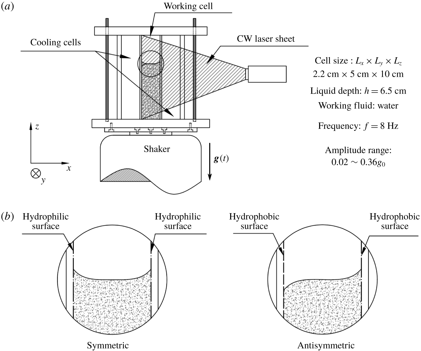
(a) Schematic drawing of the experimental apparatus. A water tank was oscillated sinusoidally in the  $z$ direction with a time-varying gravitational acceleration
 $g(t)=-(g_{0}+a_{0}\sin 2\unicode[STIX]{x03C0}f_{0}t)$. The tank was divided into three cells by two
 $\text{SiO}_{2}$ glass plates. The fluid velocity field was measured in the working cell using PIV. A DPSS laser sheet illuminated the seeding particles in the working cell at
 $y=2.5~\text{cm}$ and the particle motion was recorded by a high-speed camera. (b) Schematic of meniscus in symmetric and antisymmetric configurations.

2 Experiment
2.1 Experimental set-up
In the experiment, we used a rectangular Plexiglas tank divided into three cells by two optical glass plates (figure 1a). The middle cell was the working cell, with the dimensions  $L_{x}=2.2~\text{cm}$ in length,
 $L_{y}=5.0~\text{cm}$ in width and
 $L_{z}=10.0~\text{cm}$ in height. Deionized water filled the working cell to a depth of
 $h=6.5~\text{cm}$. Two types of meniscus symmetry were created by selecting the wettability conditions of the glass plates (see figure 1b). The clean optical glass surface was hydrophilic, with a contact angle close to
 $45^{\circ }$. A hydrophobic boundary was made by applying a coating of hydrophobic nano-
 $\text{SiO}_{2}$ film (CHEMNANO®, NC317) to an optical glass surface, creating a contact angle close to
 $135^{\circ }$. A working cell with two hydrophilic lateral boundaries creates the symmetric setting, while choosing one boundary hydrophobic and the other hydrophilic creates an antisymmetric system. We chose experiments that had contact angles closest to the ideally symmetric and antisymmetric cases. In the chosen symmetric case, the left contact angle is
 $\unicode[STIX]{x1D703}_{l}=44.01^{\circ }$ (
 $43.71^{\circ }$,
 $48.02^{\circ }$) and the right contact angle is
 $\unicode[STIX]{x1D703}_{r}=48.57^{\circ }$ (
 $46.18^{\circ }$,
 $50.75^{\circ }$). In the chosen antisymmetric case, the left contact angle is
 $\unicode[STIX]{x1D703}_{l}=142.66^{\circ }$ (
 $137.41^{\circ }$,
 $146.92^{\circ }$) and the right contact angle is
 $\unicode[STIX]{x1D703}_{r}=45.84^{\circ }$ (
 $43.65^{\circ }$,
 $47.86^{\circ }$). The numbers in parentheses are the 95 % confidence intervals. The contact angle of water with the remaining Plexiglas boundary was close to
 $90^{\circ }$.
The fluid tank was installed on an electrodynamic shaker (Labworks® ET-139) that vibrated sinusoidally in the  $z$ direction with an excess gravitational acceleration varying from
 $0.02g_{0}$ to
 $0.36g_{0}$ and a frequency of
 $f_{0}=8~\text{Hz}$. The control signal produced from a wavefunction generator was amplified using a linear power amplifier to drive the shaker. An accelerometer mounted on the base plate of the fluid tank (not shown in figure 1) measured the instantaneous acceleration, which was fed back to the wavefunction generator to regulate the control signal. The closed-loop control system reduced error and ensured the stability of the shaker oscillation.
We measured the fluid velocity field in the working cell using a particle imaging velocimetry (PIV) system. Neutrally buoyant hollow glass microspheres of diameter  $10~\unicode[STIX]{x03BC}\text{m}$ (DANTEC®, HGS-10) were seeded in the flow. Because of the effect of surface tension, some of the seeding particles were suspended on the free surface. We used these particles to track the surface deformation (see § 2.2). We found that these surface particles also played a role in enhancing surface damping and surface-deformation-induced streaming. The PIV particles in the system were illuminated from the right using a continuous, diode-pumped solid-state (DPSS) laser, creating a 1 mm thick light sheet that passed through the
 $y=2.5~\text{cm}$ plane. PIV images that cover a region from the surface to a fluid depth of approximately 3 cm were captured by a high-speed camera (Photron UX100) placed perpendicular to the laser sheet, at a frame rate of 80 Hz, achieving a time resolution of 10 frames per oscillation period. The surface oscillation caused by the primary flow is estimated by measuring the surface profile deformation in one period. Two-dimensional velocity maps for the secondary flow were obtained by cross-correlating two images with the same phase in two consecutive periods using LaVision® PIV software. Each velocity vector was calculated from interrogation windows spanning
 $32~\text{pixel}\times 32~\text{pixel}$, with 50 % overlap of neighbouring sub-windows. Each vector covers a region of
 $16~\text{pixel}\times 16~\text{pixel}$ and there are
 $80\times 64$ velocity vectors per frame, achieving a spatial resolution of 0.34 mm (one order in magnitude smaller than the capillary length scale).
The laser light sheet may heat up the fluid on the right side of the working cell and give rise to an overturning circulation. The speed of this overturning flow could be up to the order of  $O(10^{-3}~\text{cm}~\text{s}^{-1})$, comparable to the speed of the streaming flow we study. To avoid this laser-induced convection, the two lateral cells were filled with water to reduce the thermal heating of the fluid in the working cell. With this thermal protection, the speed of the overturning flow was reduced to
 $O(10^{-5}~\text{cm}~\text{s}^{-1})$ and was negligible.
2.2 Observation of the surface deformation
The time-varying acceleration of the fluid tank in the laboratory frame is  $a(t)=a_{0}\sin \unicode[STIX]{x1D711}(t)$, where
 $a_{0}$ is the forcing amplitude and
 $\unicode[STIX]{x1D711}(t)=2\unicode[STIX]{x03C0}f_{0}t$ is the oscillation phase. From Newton’s third law, the effective gravity felt by the fluid in the tank is
 $$\begin{eqnarray}g(t)=-[g_{0}+a_{0}\sin \unicode[STIX]{x1D711}(t)],\end{eqnarray}$$
in which  $g_{0}$ is the gravitational acceleration constant. When
 $\unicode[STIX]{x1D711}=\unicode[STIX]{x03C0}/2$, the fluid tank is at its highest position with maximum super-gravity; when
 $\unicode[STIX]{x1D711}=3\unicode[STIX]{x03C0}/2$, the tank is at its lowest position with maximum sub-gravity. To force the system without exciting the Faraday instability, we select
 $f_{0}=8.0~\text{Hz}$ and
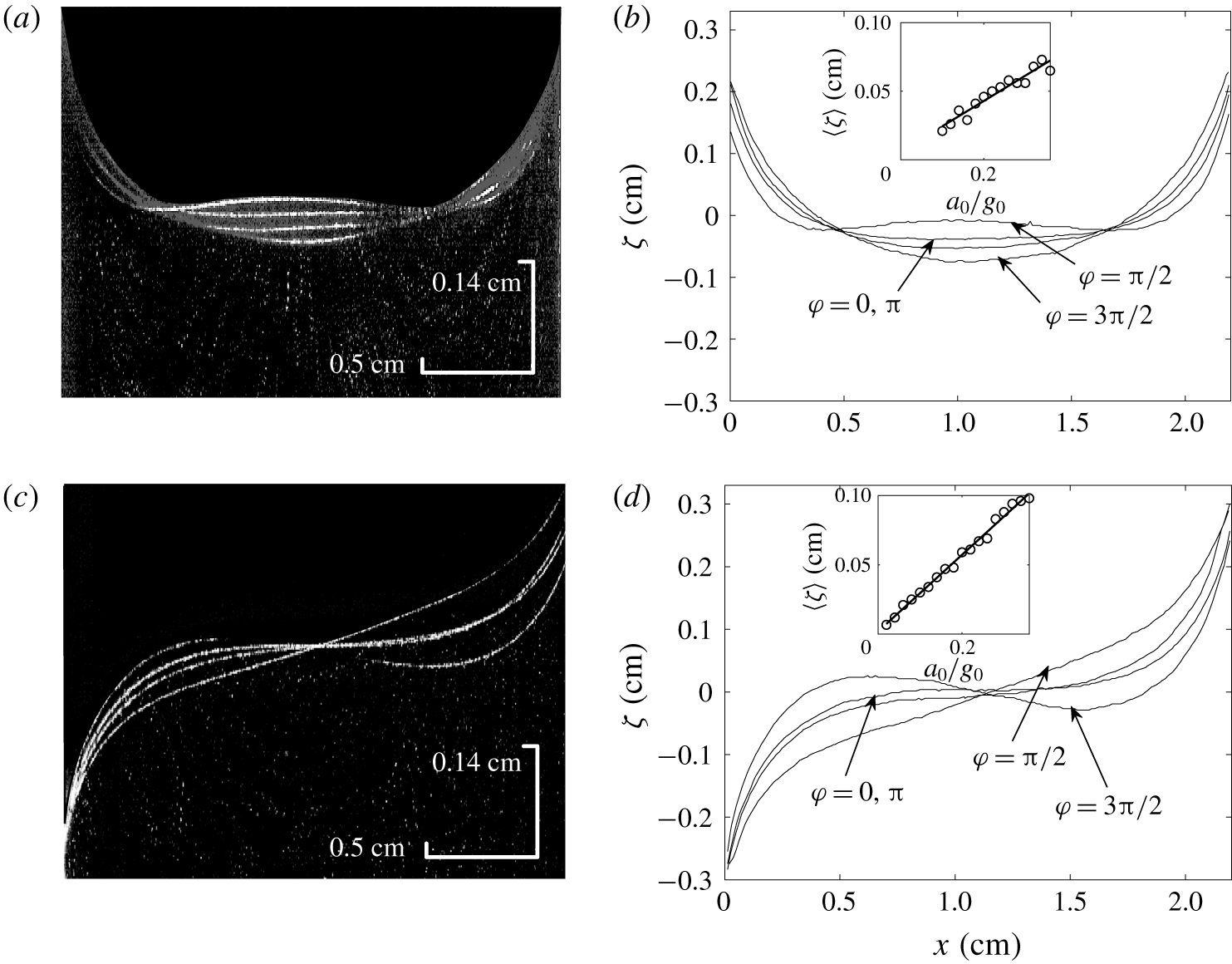
 $0.02\leqslant a_{0}/g_{0}\leqslant 0.36$ (see appendix B). Thus the periodic deformation of the liquid–air interface excites the cavity modes, giving rise to standing meniscus waves. We observe that such a surface deformation mode is strongly dependent on the geometry of the static meniscus. To quantify the relation between this surface deformation mode and the shape of the static meniscus, we measure the surface profile in different oscillation phases from the PIV images. It is found that a large proportion of the liquid–air interface is clearly visible due to seeding particles accumulated at the interface, which are illuminated by the laser sheet (figure 2a,c). The free surface is tracked using light intensity: particles are densely populated on the free surface so the light intensity is maximal there. Using this method, we extract the surface profiles
 $\unicode[STIX]{x1D701}(x)$ at four oscillatory phases,
 $\unicode[STIX]{x1D711}=0$,
 $\unicode[STIX]{x03C0}/2$,
 $\unicode[STIX]{x03C0}$ and
 $3\unicode[STIX]{x03C0}/2$, as shown in figure 2(b) and 2(d).
Images and surface profiles of meniscus shape deformation at  $\unicode[STIX]{x1D711}=0$,
 $\unicode[STIX]{x03C0}/2$,
 $\unicode[STIX]{x03C0}$ and
 $3\unicode[STIX]{x03C0}/2$, with
 $f_{0}=8~\text{Hz}$ and
 $a_{0}=0.2g_{0}$. (a) A PIV image of the vibrating surface in the symmetric configuration. (b) The extracted surface profiles corresponding to (a). (c) A PIV image of the vibrating surface in the antisymmetric configuration. (d) The extracted surface profiles of symmetric scenario corresponding to (c). The insets in (b) and (d) show the horizontally averaged surface deformation amplitude
 $\langle \unicode[STIX]{x1D701}\rangle$ as a function of
 $a_{0}/g_{0}$. The symbols in the insets are experimental measurements and the solid line is a linear regression.

The meniscus oscillates at the forcing frequency  $f_{0}$. The response of meniscus wave amplitude
 $\unicode[STIX]{x1D701}(x)$ to the forcing acceleration amplitude
 $a_{0}/g_{0}$ is estimated by the horizontally averaged surface deformation amplitude
 $\langle \unicode[STIX]{x1D701}\rangle$, which is defined by
 $$\begin{eqnarray}\langle \unicode[STIX]{x1D701}\rangle =\overline{|\unicode[STIX]{x1D701}_{\unicode[STIX]{x1D711}=\unicode[STIX]{x03C0}/2}-\unicode[STIX]{x1D701}_{\unicode[STIX]{x1D711}=3\unicode[STIX]{x03C0}/2}|},\end{eqnarray}$$
where  $\unicode[STIX]{x1D701}_{\unicode[STIX]{x1D711}=\unicode[STIX]{x03C0}/2}$ and
 $\unicode[STIX]{x1D701}_{\unicode[STIX]{x1D711}=3\unicode[STIX]{x03C0}/2}$ are the surface profiles captured at
 $\unicode[STIX]{x1D711}=\unicode[STIX]{x03C0}/2$ and
 $\unicode[STIX]{x1D711}=3\unicode[STIX]{x03C0}/2$, respectively; the overline denotes an average in the
 $x$ direction. The mean amplitude of the meniscus oscillation
 $\langle \unicode[STIX]{x1D701}\rangle$ grows linearly with the forcing amplitude (see the insets figure 2b,d). The scale for the speed of the primary flow is
 $\unicode[STIX]{x1D714}\langle \unicode[STIX]{x1D701}\rangle$, which ranges from
 $0.5~\text{cm}~\text{s}^{-1}$ to
 $5~\text{cm}~\text{s}^{-1}$. The Reynolds number for the primary flow,
 $\mathit{Re}=\unicode[STIX]{x1D714}\langle \unicode[STIX]{x1D701}\rangle L/\unicode[STIX]{x1D708}$, therefore ranges from 110 to 1100, and we can infer that the effect of viscosity on the primary oscillation is weak. In the symmetric case, the excited mode is symmetric and has two nodes. At maximum super-gravity (
 $\unicode[STIX]{x1D711}=\unicode[STIX]{x03C0}/2$) the liquid surface bulges upwards in the middle of the cell, analogous to the phenomenon of the liquid jet observed by Antkowiak et al. (Reference Antkowiak, Bremond, Le Dizès and Villermaux2007). At maximum sub-gravity (
 $\unicode[STIX]{x1D711}=3\unicode[STIX]{x03C0}/2$), the meniscus bends downwards to its greatest extent. Between these two states, the fluid flows periodically between the lateral boundary and the middle of the cell. In the antisymmetric case, an oscillatory mode with one node at the centre (
 $x=L/2$) is instead excited. When the system is at maximum sub-gravity (
 $\unicode[STIX]{x1D711}=3\unicode[STIX]{x03C0}/2$), the fluid surface forms an ‘S’ shape, with the convex part on the hydrophobic side (
 $x<L/2$) and the concave part on the hydrophilic side (
 $x>L/2$). When the system is at maximum super-gravity (
 $\unicode[STIX]{x1D711}=\unicode[STIX]{x03C0}/2$), the fluid surface approaches a straight slope. Between these two states, the fluid sloshes between the two lateral boundaries. No observable surface oscillation is found in the
 $y$ direction. Representing the mode number as
 $(k,l)$, where
 $k$ and
 $l$ are positive integers denoting the mode number on
 $x$ and
 $y$ axes, respectively, the symmetric and antisymmetric configurations give rise to mode
 $(2,0)$ and
 $(1,0)$ waves, respectively.
2.3 Observation of the streaming motion
The streaming circulation is observed when the PIV images are broadcast stroboscopically. The streaming circulation is one order of magnitude weaker than the instantaneous primary flow. Once the circulation forms, it persists as long as the forcing oscillation continues. During the experiment, we collected the PIV images one minute after the forcing was turned on, when a steady streaming circulation had been established. The flow velocity and the vertical scale of the circulations, for both wettability configurations, appear to increase if the oscillation amplitude  $a_{0}$ increases. The streaming circulation has distinct structures in symmetric and antisymmetric cases. The streaming circulation patterns are taken when
 $\unicode[STIX]{x1D711}\approx \unicode[STIX]{x03C0}$, when the free surface is close to its equilibrium state.
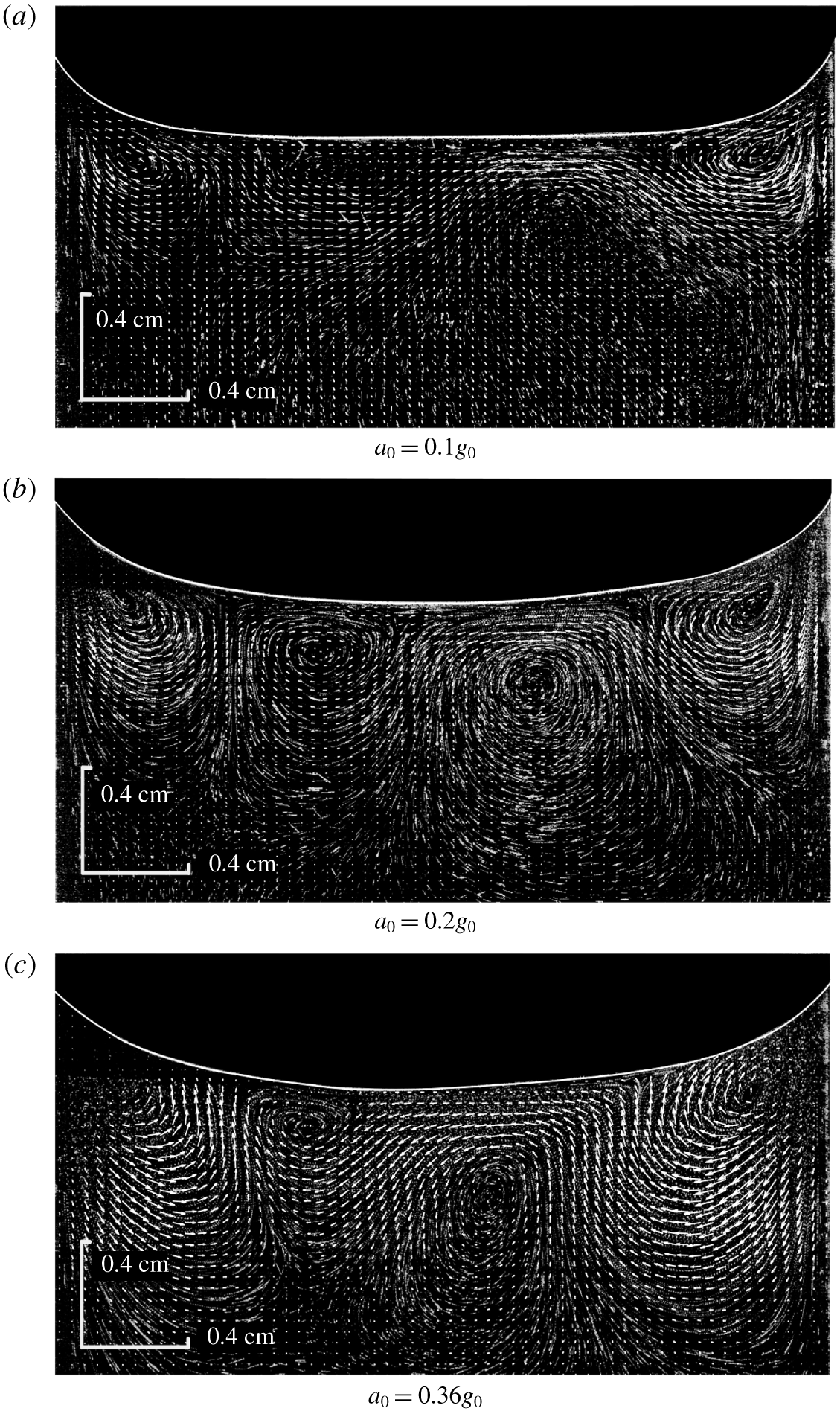
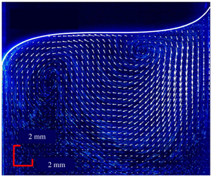
In the symmetric case (figure 3), the secondary circulation has a stable four-vortex structure, with clockwise (anticlockwise) rotation near the right (left) lateral boundary. When  $a_{0}\sim 0.1g_{0}$, the central vortices are not clearly visible in the PIV image. As the forcing gets stronger, the central vortices become apparent with approximately circular streamlines. At the strongest forcing amplitude, the boundary vortices are well developed, whereas the central vortices become suppressed and asymmetric.
Velocity fields of the streaming flows overlying the raw PIV image in the symmetric case for three values of  $a_{0}$. For each case, the driving frequency is
 $f_{0}=8~\text{Hz}$. The liquid–air interface has been highlighted manually. The streaming flows in (a), (b) and (c) are computed at the oscillation phases
 $\unicode[STIX]{x1D711}=9/10\unicode[STIX]{x03C0}$,
 $\unicode[STIX]{x1D711}=13/10\unicode[STIX]{x03C0}$ and
 $\unicode[STIX]{x1D711}=13/10\unicode[STIX]{x03C0}$, respectively.

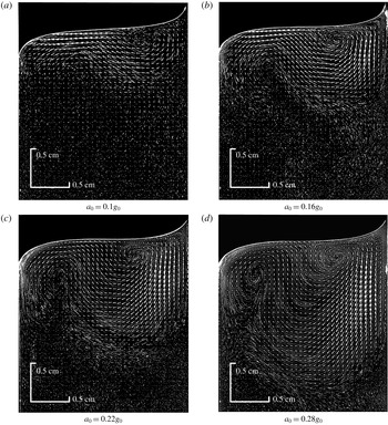
In the antisymmetric case, the secondary flow field has a dipole circulation structure with a weaker anticlockwise circulation near the hydrophobic side and a stronger clockwise circulation near the hydrophilic side (figure 4). When the forcing is weak,  $a_{0}\sim 0.1g_{0}$, the anticlockwise circulation is only partially visible in the PIV image, but a strong leftward velocity is found below the free surface. As the forcing amplitude increases, the anticlockwise circulation becomes more dominant and downward motion becomes more prominent near the hydrophobic side.
Velocity fields of the streaming flows overlying the raw PIV image in the antisymmetric case for four values of  $a_{0}$. For each case, the driving frequency is
 $f_{0}=8~\text{Hz}$. The liquid–air interface has been highlighted manually. The streaming flows in (a), (b), (c) and (d) are computed at the oscillation phases
 $\unicode[STIX]{x1D711}=5/6\unicode[STIX]{x03C0}$,
 $\unicode[STIX]{x1D711}=9/10\unicode[STIX]{x03C0}$,
 $\unicode[STIX]{x1D711}=9/10\unicode[STIX]{x03C0}$ and
 $11/10\unicode[STIX]{x03C0}$, respectively.

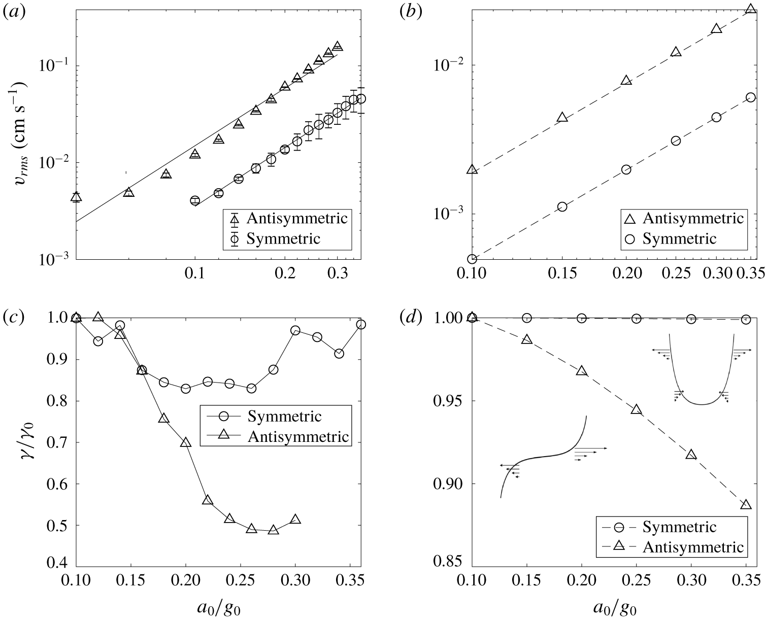
Response of the (a,b) r.m.s. speed,  $v_{rms}$, and (c,d) symmetry parameter,
 $\unicode[STIX]{x1D6FE}/\unicode[STIX]{x1D6FE}_{0}$, to changes in forcing amplitude
 $a_{0}/g_{0}$ in (a,c) the laboratory experiments and (b,d) the simulations. The fitted trends in (a) have
 $\unicode[STIX]{x1D6FD}=2.02$ and
 $\unicode[STIX]{x1D6FD}=1.97$ for symmetric and antisymmetric cases, respectively, while the fitted trends in (b) both have
 $\unicode[STIX]{x1D6FD}=2.0$. The symmetry parameter
 $\unicode[STIX]{x1D6FE}$ is defined in (2.3) and normalized by
 $\unicode[STIX]{x1D6FE}_{0}=\unicode[STIX]{x1D6FE}|_{a_{0}/g_{0}=0.1}$. The insets in (d) show schematic plots illustrating the streaming velocity distribution under the free surface.

To quantify the dynamical behaviour of the secondary flow, we compute the r.m.s. fluid speed in the observed section:
 $$\begin{eqnarray}\displaystyle v_{rms}=\frac{1}{A}\sqrt{\iint _{A}(u^{2}+w^{2})\,\text{d}x\,\text{d}z}. & & \displaystyle\end{eqnarray}$$
Here  $A$ is the total cross-sectional area of the observed fluid bulk, and
 $u$ and
 $w$ are the velocity components in the
 $x$ and
 $z$ directions, respectively. As shown in figure 5(a), the kinetic energy density for fully established secondary flow structure
 $v_{rms}$ scales like
 $$\begin{eqnarray}\displaystyle v_{rms}\sim (a_{0}/g_{0})^{\unicode[STIX]{x1D6FD}}, & & \displaystyle\end{eqnarray}$$
where  $\unicode[STIX]{x1D6FD}\approx 2$ for both symmetric and antisymmetric cases. This indicates that the secondary circulation is caused by the quadratic nonlinearity of the velocity field, which is consistent with the direct numerical simulations of Carrión et al. (Reference Carrión, Herrada, Montanero and Vega2017). Note that the flow velocity near the boundary is not resolvable by PIV, so the integration in (2.1) excludes the region within 0.034 cm of the lateral boundaries. Further, the camera does not capture the whole water bulk, so the integration covers the region
 $z>-1.79~\text{cm}$ in the symmetric case and
 $z>-1.65~\text{cm}$ in the antisymmetric case. To avoid edge effects from the bottom, we limit the maximum forcing amplitude so that the streaming velocity at the bottom edge of the observation window is never more than 10 % of the characteristic secondary flow speed in the bulk.
The spatial symmetry of the secondary circulation pattern is quantified by the symmetry parameter
 $$\begin{eqnarray}\displaystyle \unicode[STIX]{x1D6FE}=\frac{\displaystyle \iint _{x<L/2}\,\text{d}x\,\text{d}z\,|\unicode[STIX]{x1D6FA}(x,z)|/A_{x<L/2}}{\displaystyle \iint _{x>L/2}\,\text{d}x\,\text{d}z\,|\unicode[STIX]{x1D6FA}(x,z)|/A_{x>L/2}}, & & \displaystyle\end{eqnarray}$$
which denotes the ratio of mean vorticity magnitude of the left region over that of the right region of the working cell. In (2.3),  $|\unicode[STIX]{x1D6FA}(x,z)|$ is the magnitude of the vorticity, and
 $A_{x>L/2}$ and
 $A_{x<L/2}$ are the liquid bulk areas at the right or left side, respectively, of
 $x=1.1~\text{cm}$ below the static meniscus. Figure 5(b,d) shows the variation of
 $\unicode[STIX]{x1D6FE}/\unicode[STIX]{x1D6FE}_{0}$ against
 $a_{0}/g_{0}$, where
 $\unicode[STIX]{x1D6FE}_{0}=\unicode[STIX]{x1D6FE}|_{a_{0}/g_{0}=0.1}$ is a reference
 $\unicode[STIX]{x1D6FE}$ value. The variation of
 $\unicode[STIX]{x1D6FE}/\unicode[STIX]{x1D6FE}_{0}$ with forcing amplitude is different in the symmetric and antisymmetric cases. In the symmetric case, the secondary flows remains highly symmetric, with no obvious trend in
 $\unicode[STIX]{x1D6FE}/\unicode[STIX]{x1D6FE}_{0}$. In contrast, in the antisymmetric case, the symmetry parameter
 $\unicode[STIX]{x1D6FE}$ decreases rapidly as the forcing amplitude increases, then saturates at
 $\unicode[STIX]{x1D6FE}\approx 0.5\unicode[STIX]{x1D6FE}_{0}$ for large forcing amplitudes.
3 Theory
In this section, we develop a theoretical description of the meniscus wave and resulting secondary circulation. In order to simplify the analysis, we assume that the imaged flow is two-dimensional (2-D); that is, we neglect the effect of the front and back plates. We start by deriving the static shape of the meniscus and solve for the wave modes on this background state in § 3.1. The secondary circulation is obtained in § 3.2 by determining the streaming circulation along the free surface and lateral boundaries and using these as boundary conditions for a steady hydrodynamics solver.
3.1 Meniscus wave
The meniscus wave is solved by linearization of the ideal fluid equations with a free surface (e.g. Batchelor Reference Batchelor2000). The nonlinear fluid equations are
 $$\begin{eqnarray}\displaystyle & \displaystyle \unicode[STIX]{x1D6FB}^{2}\unicode[STIX]{x1D719}=0, & \displaystyle\end{eqnarray}$$
 $$\begin{eqnarray}\displaystyle & \displaystyle \left.\left[\unicode[STIX]{x2202}_{t}\unicode[STIX]{x1D719}+\frac{1}{2}(\unicode[STIX]{x1D735}\unicode[STIX]{x1D719})^{2}\right]\right|_{z=\unicode[STIX]{x1D701}}+[g_{0}+a_{0}\sin (\unicode[STIX]{x1D714}t)]\unicode[STIX]{x1D701}=\frac{\unicode[STIX]{x1D70E}}{\unicode[STIX]{x1D70C}}\frac{\unicode[STIX]{x2202}_{xx}^{2}\unicode[STIX]{x1D701}}{[1+(\unicode[STIX]{x2202}_{x}\unicode[STIX]{x1D701})^{2}]^{3/2}}, & \displaystyle\end{eqnarray}$$
 $$\begin{eqnarray}\displaystyle & \displaystyle \unicode[STIX]{x2202}_{t}\unicode[STIX]{x1D701}+\unicode[STIX]{x2202}_{x}\unicode[STIX]{x1D719}|_{z=\unicode[STIX]{x1D701}}\unicode[STIX]{x2202}_{x}\unicode[STIX]{x1D701}=\unicode[STIX]{x2202}_{z}\unicode[STIX]{x1D719}|_{z=\unicode[STIX]{x1D701}}, & \displaystyle\end{eqnarray}$$
 $$\begin{eqnarray}\displaystyle & \displaystyle \unicode[STIX]{x1D719}|_{z\rightarrow -\infty }=0, & \displaystyle\end{eqnarray}$$
 $$\begin{eqnarray}\displaystyle & \displaystyle \unicode[STIX]{x2202}_{x}\unicode[STIX]{x1D719}|_{x=0,L}=0, & \displaystyle\end{eqnarray}$$
where  $\unicode[STIX]{x1D701}=\unicode[STIX]{x1D701}(x,t)$ is the surface elevation and
 $\unicode[STIX]{x1D719}=\unicode[STIX]{x1D719}(x,z,t)$ is the velocity potential field. The parameter notation is the same as in the previous section. The cell width is
 $L=2.2~\text{cm}$,
 $g_{0}=980~\text{cm}~\text{s}^{-2}$ is the gravitational acceleration,
 $\unicode[STIX]{x1D70C}=1~\text{g}~\text{cm}^{-3}$ is the density of water,
 $\unicode[STIX]{x1D70E}=72~\text{dyne}~\text{cm}^{-1}$ is the surface tension of water,
 $a_{0}$ is the forcing acceleration, and
 $\unicode[STIX]{x1D714}=2\unicode[STIX]{x03C0}f_{0}$ is the forcing angular frequency.
The linearization is done in the following way. We use the capillary length  $l_{c}=\sqrt{\unicode[STIX]{x1D70E}/(\unicode[STIX]{x1D70C}g_{0})}=0.27~\text{cm}$ as the characteristic length scale in the
 $x$ and
 $z$ directions. The scale of the surface displacement due to the forced oscillation is
 $a_{0}/\unicode[STIX]{x1D714}^{2}\approx 0.008{-}0.13~\text{cm}$, so the ratio between these two length scales is a small dimensionless number,
 $\unicode[STIX]{x1D716}=a_{0}/(l_{c}\unicode[STIX]{x1D714}^{2})\approx 0.03{-}0.5$, that scales the linear system response. In the experiment, the dimensionless forcing strength
 $a_{0}/g_{0}$ has the magnitude range of
 $0.02{-}0.36$, which is
 $O(\unicode[STIX]{x1D716})$. The mean static surface slope
 $\unicode[STIX]{x2202}_{x}\unicode[STIX]{x1D701}_{0}$ approaches zero at
 $x=1.1~\text{cm}$ and
 ${\approx}1$ at both boundaries. Nevertheless, to make progress, we assume that
 $\unicode[STIX]{x2202}_{x}\unicode[STIX]{x1D701}_{0}\sim O(\unicode[STIX]{x1D716})$ everywhere, while acknowledging that this will lead to errors near the boundaries. After scaling the velocity potential,
 $\unicode[STIX]{x1D719}$, by
 $g_{0}a_{0}/\unicode[STIX]{x1D714}^{3}$, the solution of the ideal fluid equations (3.1)–(3.5) can be expanded in an asymptotic series in powers of
 $\unicode[STIX]{x1D716}$:
 $$\begin{eqnarray}\displaystyle & \unicode[STIX]{x1D701}=\unicode[STIX]{x1D701}_{0}+\unicode[STIX]{x1D701}_{1}, & \displaystyle\end{eqnarray}$$
 $$\begin{eqnarray}\displaystyle & \unicode[STIX]{x1D719}=\unicode[STIX]{x1D719}_{0}+\unicode[STIX]{x1D719}_{1}. & \displaystyle\end{eqnarray}$$
The quantities with the subscript 0 are  $O(1)$, which represents a situation when the forcing is neglected and depicts the static balance in the fluid bulk. Thus, both
 $\unicode[STIX]{x1D719}_{0}$ and
 $\unicode[STIX]{x1D701}_{0}$ are independent of time. The quantities with subscript 1, that is,
 $O(\unicode[STIX]{x1D716})$, represent the linear wave forced by the vertical oscillation. As the depth is three times larger than the cell width, we apply an infinite-depth bottom boundary condition.
3.1.1 Zeroth-order solution
At  $O(1)$, equations (3.1) and (3.2) become the Young–Laplace equation:
 $$\begin{eqnarray}\displaystyle \unicode[STIX]{x2202}_{xx}^{2}\unicode[STIX]{x1D701}_{0}=\frac{\unicode[STIX]{x1D70C}g_{0}}{\unicode[STIX]{x1D70E}}(\unicode[STIX]{x1D701}_{0}-z^{\ast }). & & \displaystyle\end{eqnarray}$$
Since the left plate and right plate completely prevent liquid mass exchange, the experiment is done with total fluid volume conserved. The reference elevation,
 $$\begin{eqnarray}z^{\ast }=-\frac{\unicode[STIX]{x1D70E}}{\unicode[STIX]{x1D70C}g_{0}L}(\unicode[STIX]{x2202}_{x}\unicode[STIX]{x1D701}_{0}|_{x=L}-\unicode[STIX]{x2202}_{x}\unicode[STIX]{x1D701}_{0}|_{x=0})=-\frac{\unicode[STIX]{x1D70E}}{\unicode[STIX]{x1D70C}g_{0}L}[\tan (\unicode[STIX]{x1D703}_{r})-\tan (\unicode[STIX]{x03C0}/2-\unicode[STIX]{x1D703}_{l})],\end{eqnarray}$$
is determined by integrating equation (3.8) in  $x$, applying the lateral boundary conditions, and requiring that the horizontal integral of
 $\unicode[STIX]{x1D701}_{0}$ vanish. The quantities
 $\unicode[STIX]{x1D703}_{l}$ and
 $\unicode[STIX]{x1D703}_{r}$ are the contact angles at the left and right boundaries, respectively. Following the experimental set-up, in the symmetric case
 $\unicode[STIX]{x1D703}_{l}=\unicode[STIX]{x1D703}_{r}=45^{\circ }$, and in the antisymmetric case
 $\unicode[STIX]{x1D703}_{l}=135^{\circ }$ and
 $\unicode[STIX]{x1D703}_{r}=45^{\circ }$. The corresponding boundary conditions for (3.8) are written as
 $$\begin{eqnarray}\displaystyle & \unicode[STIX]{x2202}_{x}\unicode[STIX]{x1D701}_{0}|_{x=0}=-s, & \displaystyle\end{eqnarray}$$
 $$\begin{eqnarray}\displaystyle & \unicode[STIX]{x2202}_{x}\unicode[STIX]{x1D701}_{0}|_{x=L}=1. & \displaystyle\end{eqnarray}$$
Here,  $s$ controls the symmetry of the meniscus; it is 1 in the symmetric case and
 $-1$ in the antisymmetric case. These boundary conditions and the above zeroth-order equation are satisfied by
 $$\begin{eqnarray}\displaystyle \unicode[STIX]{x1D701}_{0}=\frac{1+s\cosh (mL)}{m\sinh (mL)}\cosh (mx)-\frac{s}{m}\sinh (mx)+z^{\ast }, & & \displaystyle\end{eqnarray}$$
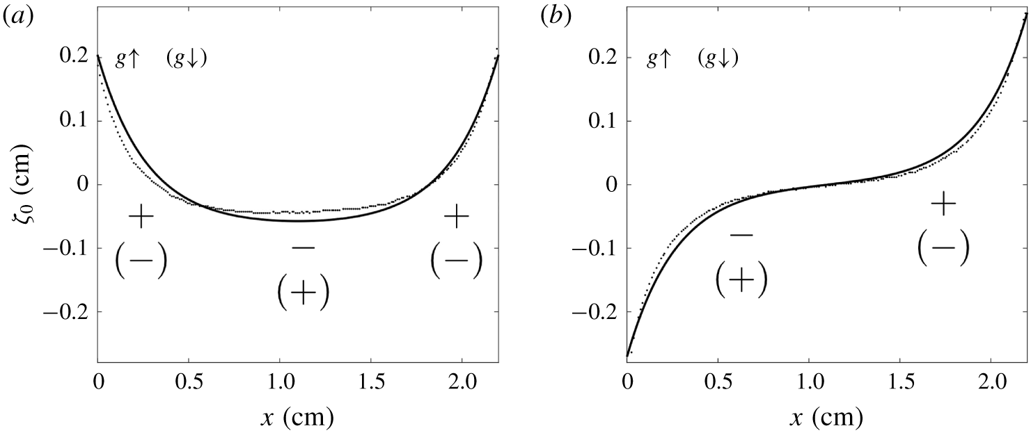
where  $m=l_{c}^{-1}$. In figure 7, the solutions are compared to the static surface profile measurements for both symmetric and antisymmetric cases – the theoretical result captures the shape of the free surface well.
The zeroth-order meniscus solution  $\unicode[STIX]{x1D701}_{0}$ (solid line) compared to the experimental measurement (dotted line) for (a) symmetric and (b) antisymmetric cases. The
 $+$ and
 $-$ signs represent the surplus and deficit of dynamical pressure
 $p_{d}$, respectively, that arises when the acceleration is changed by
 $a_{0}\unicode[STIX]{x1D714}\unicode[STIX]{x1D6FF}t$, where
 $\unicode[STIX]{x1D6FF}t$ is a small time increment. The
 $p_{d}$ distribution outside (inside) of the bracket is for the situation when
 $g$ is increased (decreased).

3.1.2 First-order solution
At  $O(\unicode[STIX]{x1D716})$, the governing equations and boundary conditions become
 $$\begin{eqnarray}\displaystyle & \displaystyle \unicode[STIX]{x1D6FB}^{2}\unicode[STIX]{x1D719}_{1}=0, & \displaystyle\end{eqnarray}$$
 $$\begin{eqnarray}\displaystyle & \displaystyle \unicode[STIX]{x2202}_{t}\unicode[STIX]{x1D719}_{1}|_{z=0}+g_{0}\unicode[STIX]{x1D701}_{1}-\frac{\unicode[STIX]{x1D70E}}{\unicode[STIX]{x1D70C}}\unicode[STIX]{x2202}_{xx}^{2}\unicode[STIX]{x1D701}_{1}=-a_{0}\unicode[STIX]{x1D701}_{0}\sin (\unicode[STIX]{x1D714}t), & \displaystyle\end{eqnarray}$$
 $$\begin{eqnarray}\displaystyle & \displaystyle \unicode[STIX]{x2202}_{z}\unicode[STIX]{x1D719}_{1}|_{z=0}-\unicode[STIX]{x2202}_{t}\unicode[STIX]{x1D701}_{1}=0, & \displaystyle\end{eqnarray}$$
 $$\begin{eqnarray}\displaystyle & \displaystyle \unicode[STIX]{x1D719}_{1}|_{z=-\infty }=0, & \displaystyle\end{eqnarray}$$
 $$\begin{eqnarray}\displaystyle & \displaystyle \unicode[STIX]{x2202}_{x}\unicode[STIX]{x1D719}_{1}|_{x=0,L}=0. & \displaystyle\end{eqnarray}$$
The first-order surface pressure balance (3.14) suggests a physical interpretation for the mechanism of the meniscus wave. Suppose that the system is initially at rest, so that  $\unicode[STIX]{x1D701}_{1}=0$, and the vertical acceleration increases by an amount
 $\unicode[STIX]{x1D6FF}g=a_{0}\unicode[STIX]{x1D714}\unicode[STIX]{x1D6FF}t$ over the background value
 $g_{0}$. At this instant, the dynamic pressure is
 $$\begin{eqnarray}p_{d}=-\unicode[STIX]{x1D70C}\unicode[STIX]{x2202}_{t}\unicode[STIX]{x1D719}_{1}|_{z=0}=\unicode[STIX]{x1D70C}\unicode[STIX]{x1D6FF}g\unicode[STIX]{x1D701}_{0},\end{eqnarray}$$
so that there is an excess of dynamic pressure where  $\unicode[STIX]{x1D701}_{0}>0$ and a deficit where
 $\unicode[STIX]{x1D701}_{0}<0$. In the symmetric case, this dynamic pressure perturbation will cause the free surface to fall in the centre of the cell and rise on the sides, leading to a wave with two nodes (figure 6a). For the antisymmetric case, the same process will cause the free surface to fall and rise on the left and right, respectively, sides of the cell, so the meniscus wave will have a single node (figure 6b). A decrease in the vertical acceleration will lead to the opposite pattern of dynamic pressure perturbations, resulting in the opposite surface deflection.
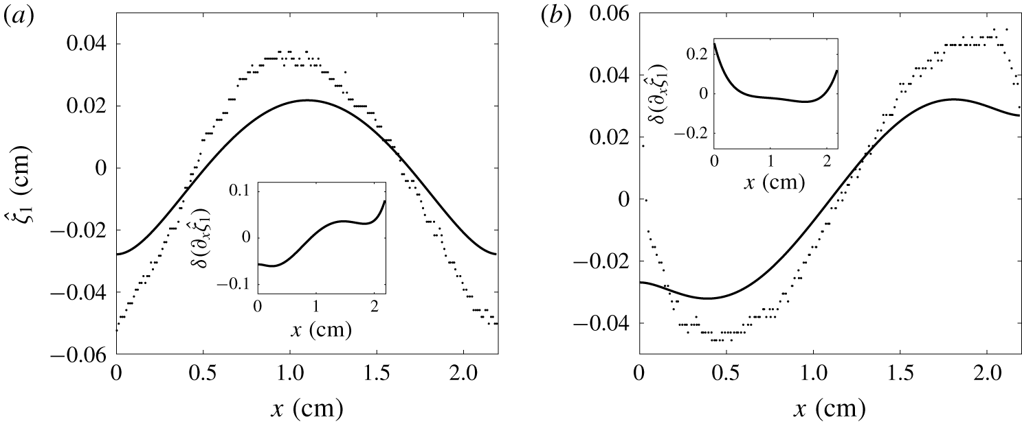
The first-order meniscus solutions  $\hat{\unicode[STIX]{x1D701}}_{1}$ (solid line) compared to the experimental measurements (dotted line) when
 $a_{0}=0.2g_{0}$ and
 $f_{0}=8~\text{Hz}$ for (a) the symmetric and (b) the antisymmetric cases. The experimental
 $\hat{\unicode[STIX]{x1D701}}_{1}$ are produced by subtracting the static surface profiles from the oscillating surface profiles captured during the slack phase. The insets show the difference between the theoretical first-order slope and the experimental first-order slope,
 $\unicode[STIX]{x1D6FF}(\unicode[STIX]{x2202}_{x}\hat{\unicode[STIX]{x1D701}}_{1})$.

The solution that satisfies (3.13)–(3.17) takes the form
 $$\begin{eqnarray}\displaystyle & \displaystyle \unicode[STIX]{x1D719}_{1}=\hat{\unicode[STIX]{x1D719}}_{1}\cos (\unicode[STIX]{x1D714}t)=\mathop{\sum }_{n=1}^{\infty }A_{n}\text{e}^{k_{n}z}\cos (k_{n}x)\cos (\unicode[STIX]{x1D714}t), & \displaystyle\end{eqnarray}$$
 $$\begin{eqnarray}\displaystyle & \displaystyle \unicode[STIX]{x1D701}_{1}=\hat{\unicode[STIX]{x1D701}}_{1}\sin (\unicode[STIX]{x1D714}t)=\mathop{\sum }_{n=1}^{\infty }\frac{A_{n}k_{n}}{\unicode[STIX]{x1D714}}\cos (k_{n}x)\sin (\unicode[STIX]{x1D714}t), & \displaystyle\end{eqnarray}$$
where the eigen-wavenumber  $k_{n}=n\unicode[STIX]{x03C0}/L$ and coefficients
 $A_{n}$ are given by
 $$\begin{eqnarray}\displaystyle A_{n}=\frac{2\unicode[STIX]{x1D714}a_{0}}{\unicode[STIX]{x1D714}^{2}-\unicode[STIX]{x1D714}_{n}^{2}}\frac{(-1)^{n}+s}{(m^{2}+k_{n}^{2})L}, & & \displaystyle\end{eqnarray}$$
where
 $$\begin{eqnarray}\displaystyle \unicode[STIX]{x1D714}_{n}^{2}=g_{0}k_{n}(1+k_{n}^{2}l_{c}^{2}) & & \displaystyle\end{eqnarray}$$
is the (squared) natural frequency of a capillary–gravity wave with wavenumber  $k_{n}$. Note that these wave modes (3.19) and (3.20) are not parametric resonance modes (Faraday modes), but ordinary resonance modes, since they have the same frequency as the forcing. The wave energy is concentrated around those
 $n$ for which
 $\unicode[STIX]{x1D714}_{n}$ is close to
 $\unicode[STIX]{x1D714}$. If
 $\unicode[STIX]{x1D714}=\unicode[STIX]{x1D714}_{n}$, for a given
 $n$, the capillary–gravity wave can travel integer multiples of the cell length during one forcing cycle. For a particular wave mode
 $n$ and oscillation frequency
 $\unicode[STIX]{x1D714}$, the mode amplitude
 $A_{n}$ is also controlled by the distance between the boundary plates
 $L$. When the resonance condition
 $\unicode[STIX]{x1D714}=\unicode[STIX]{x1D714}_{n}(L)$ is satisfied by tuning
 $L$, the mode amplitude
 $A_{n}\rightarrow \infty$. The mode amplitude
 $A_{n}$ goes to zero like
 $L^{-1}$ as
 $L\rightarrow \infty$ and like
 $L^{4}$ as
 $L\rightarrow 0$. The forcing frequency
 $f_{0}=8~\text{Hz}$ is approximately at the midpoint between two flat-surface resonant frequencies,
 $f_{1}=6.38~\text{Hz}$ and
 $f_{2}=10.65~\text{Hz}$, for modes
 $n=1$ and
 $n=2$, respectively. If the equilibrium surface were flat, the amplitudes
 $A_{1}$ and
 $A_{2}$ would be comparable to each other. However, the (anti)symmetry of the equilibrium surface selects excitations with the corresponding (anti)symmetry:
 $A_{1}=0$ in the symmetric case and
 $A_{2}=0$ in the antisymmetric case (see (3.21)). The amplitude
 $A_{n}$ decays like
 $O(n^{-5})$, so the series converges quickly. In figure 7, the infinite series is terminated at
 $n=200$ to produce the estimate of the meniscus wave amplitude
 $\hat{\unicode[STIX]{x1D701}}_{1}$ for both symmetric and antisymmetric cases.
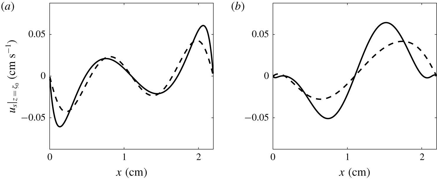
The streaming flow velocity along the free surface at  $\unicode[STIX]{x1D711}=\unicode[STIX]{x03C0}$, when
 $a_{0}=0.2g_{0}$ and
 $f_{0}=8~\text{Hz}$ for (a) the symmetric and (b) the antisymmetric cases. The solid line is the result (3.26) truncated at
 $m+n=200$, while the dashed line contains contributions from the gravest mode only.

In figure 7, the experimental wave amplitudes are 67 % and 42 % larger than the theoretical values for the symmetric and antisymmetric cases, respectively. The linearized theory is inadequate to produce a more accurate result, because our basic scaling approximation  $\unicode[STIX]{x2202}_{x}(\unicode[STIX]{x1D701}_{0}+\unicode[STIX]{x1D701}_{1})\rightarrow 0$ is not satisfied since
 $\unicode[STIX]{x2202}_{x}\unicode[STIX]{x1D701}_{0}\sim 1$ near the contact angle. The insets in figure 7 show the differences between the theoretical and experimental first-order slopes,
 $\unicode[STIX]{x1D6FF}(\unicode[STIX]{x2202}_{x}\hat{\unicode[STIX]{x1D701}}_{1})$. The experimental slope is determined by fitting a fifth-order polynomial to the measured
 $\hat{\unicode[STIX]{x1D701}}_{1}$ profile. We can see that
 $\unicode[STIX]{x1D6FF}(\unicode[STIX]{x2202}_{x}\hat{\unicode[STIX]{x1D701}}_{1})$ is large near the contact line and zero near the centre of the cell.
The deviation between the experiment and theory may also due to the contact-line dynamics. In the theory, the contact line is assumed to be free-slipping with the liquid body. In the experimental measurement shown in figure 8, the amplitude of the oscillation near the contact line is larger (smaller) than predicted in the symmetric (antisymmetric) case. These interesting behaviours may contribute to the difference between the predicted and observed meniscus wave shapes. Nevertheless, a precise analytical model of the meniscus wave is not the main purpose of this work. In the next section, we will show that the meniscus wave solution obtained here is sufficient to explain the streaming circulation pattern formation.
3.2 Streaming circulation
In this section, we explain the secondary circulation pattern shown in figures 3 and 4. Firstly, we note that the surface appears to play a very important role in streaming circulation generation, since the number of secondary vortices doubles as the dominant mode number of the meniscus wave flow doubles. Moreover, the nodes of the meniscus wave are above upwelling flow, while the antinodes cap downwelling flows. The spatial relationships between the meniscus wave and the streaming flow indicate that the streaming flow is generated by the meniscus wave itself. This streaming flow affects the bulk through viscous momentum transfer, so as to generate a secondary circulation pattern.
The fluid surface was not frequently cleaned during the experiments, which leads to the build-up of surface contamination. The free surface is additionally contaminated by a large number of seeding particles which form a membrane (see figure 2). Under these conditions, the free surface acts like a no-slip boundary (Henderson & Segur Reference Henderson and Segur2013; Moisy et al. Reference Moisy, Bouvard and Herreman2018). We therefore treat the free surface as a vibrating solid when applying the streaming theory of Nicolás & Vega (Reference Nicolás and Vega2003).
3.2.1 Streaming under the free surface
Let the primary-flow-induced deflection normal to the unperturbed boundary,  $f$, the primary-flow oscillation along the boundary,
 $u_{\Vert }$, and the tangential boundary-oscillation velocity,
 $v^{w}$, be written as
 $$\begin{eqnarray}\displaystyle & f=F\text{e}^{\text{i}\unicode[STIX]{x1D714}t}+\text{c.c.}, & \displaystyle \nonumber\\ \displaystyle & u_{\Vert }=U\text{e}^{\text{i}\unicode[STIX]{x1D714}t}+\text{c.c.}, & \displaystyle \nonumber\\ \displaystyle & v^{w}=U^{w}\text{e}^{\text{i}\unicode[STIX]{x1D714}t}+\text{c.c.}, & \displaystyle \nonumber\end{eqnarray}$$
where  $F$ is the normal oscillation amplitude and
 $U^{w}$ is the tangential velocity amplitude of the boundary. With the present notation, the streaming velocity along a vibrating solid boundary in two dimensions is given by equations (6.2) of Nicolás & Vega (Reference Nicolás and Vega2003):
 $$\begin{eqnarray}\displaystyle u_{\bot }^{s}=\unicode[STIX]{x2202}_{\unicode[STIX]{x1D70F}}(F^{\ast }U)+\text{c.c.}, & & \displaystyle\end{eqnarray}$$
 $$\begin{eqnarray}\displaystyle u_{\Vert }^{s} & = & \displaystyle \unicode[STIX]{x1D705}F^{\ast }(2U-3U^{w})-\text{i}\unicode[STIX]{x1D714}F^{\ast }\unicode[STIX]{x2202}_{\unicode[STIX]{x1D70F}}F-\frac{3}{2\unicode[STIX]{x1D714}}[(U^{\ast }-U^{w\ast })\unicode[STIX]{x2202}_{\unicode[STIX]{x1D70F}}(U-U^{w})]\nonumber\\ \displaystyle & & \displaystyle -\,\frac{\text{i}}{\unicode[STIX]{x1D714}}[(3U-5U^{w})\unicode[STIX]{x2202}_{\unicode[STIX]{x1D70F}}U^{\ast }]-\frac{1}{\unicode[STIX]{x1D714}}(3U-U^{w})\unicode[STIX]{x2202}_{\unicode[STIX]{x1D70F}}U^{w\ast }+\text{c.c.},\end{eqnarray}$$
where  $\unicode[STIX]{x2202}_{\unicode[STIX]{x1D70F}}$ is the derivative along the steady meniscus,
 $u_{\bot }^{s}$ and
 $u_{\Vert }^{s}$ are the streaming velocity normal and parallel to the steady meniscus, respectively,
 $\unicode[STIX]{x1D705}\approx \unicode[STIX]{x2202}_{xx}^{2}\unicode[STIX]{x1D701}_{0}$ is the curvature of the unperturbed boundary, and
 $U$ is the oscillation amplitude of the primary flow tangential to the steady free surface. According to our approximation
 $\unicode[STIX]{x2202}_{x}\unicode[STIX]{x1D701}_{0}\rightarrow 0$, the tangential sliding of the unperturbed surface is negligible and we have
 $f\approx \unicode[STIX]{x1D701}_{1}$ and
 $v^{w}\approx 0$.
The results (3.23) and (3.24) are independent of the oscillation phase, since the result is evaluated at the unperturbed boundary (equivalent to  $\unicode[STIX]{x1D711}=\unicode[STIX]{x03C0}$ in our case) and averaged over one period. For a standing wave, the normal deformation amplitude,
 $f$, and primary-flow velocity amplitude parallel to the free surface,
 $u_{\Vert }$, are given by
 $$\begin{eqnarray}\displaystyle & \displaystyle f\approx \hat{\unicode[STIX]{x1D701}}_{1}\sin (\unicode[STIX]{x1D714}t)=\frac{\hat{\unicode[STIX]{x1D701}_{1}}}{2\text{i}}(\text{e}^{\text{i}\unicode[STIX]{x1D714}t}-\text{e}^{-\text{i}\unicode[STIX]{x1D714}t}), & \displaystyle \nonumber\\ \displaystyle & \displaystyle u_{\Vert }=u_{\Vert }\cos (\unicode[STIX]{x1D714}t)=\frac{\hat{u} _{\Vert }}{2}(\text{e}^{\text{i}\unicode[STIX]{x1D714}t}+\text{e}^{-\text{i}\unicode[STIX]{x1D714}t}), & \displaystyle \nonumber\end{eqnarray}$$
where  $\hat{\unicode[STIX]{x1D701}}_{1}$ and
 $\hat{u} _{\Vert }$ are real functions, so that
 $F$ and
 $U$ are given by
 $$\begin{eqnarray}\displaystyle F=\frac{\hat{\unicode[STIX]{x1D701}_{1}}}{2i},\quad U=\frac{\hat{u} _{\Vert }}{2}. & & \displaystyle \nonumber\end{eqnarray}$$
Substitution of  $F$,
 $U$ and
 $U^{w}$ into (3.23) and (3.24) gives
 $$\begin{eqnarray}\displaystyle \boldsymbol{u}_{s}|_{z=\unicode[STIX]{x1D701}_{0}}=-\frac{3}{4\unicode[STIX]{x1D714}}\hat{u} _{\Vert }\unicode[STIX]{x2202}_{\unicode[STIX]{x1D70F}}\hat{u} _{\Vert }\hat{\boldsymbol{t}}, & & \displaystyle\end{eqnarray}$$
where  $\hat{\boldsymbol{t}}$ is the tangential unit vector along the meniscus. Note that, since the surface elevation is
 $90^{\circ }$ out of phase with the flow field, the streaming flow normal to the meniscus surface
 $u_{\bot }^{s}=0$. Moreover, the tangential streaming flow components proportional to the curvature
 $\unicode[STIX]{x1D705}$ and surface deformation
 $F$ do not appear in the final result, which is of the same form as for an undeformable solid surface (Nicolás & Vega Reference Nicolás and Vega2003). Although the term
 ${\sim}\unicode[STIX]{x1D705}FU$ disappears in our system, its physical meaning is of interest. When there is a local curvature on the unperturbed free surface, the perpendicular deformation shrinks the curve element length in the curvature direction. Thus the boundary viscous stress does more (less) work at the phases when the surface curve element stretches (shrinks). For progressive waves, when the velocity oscillation along the surface is in phase with the normal deformation, the damping asymmetry within one period produces a net Eulerian flow. For standing waves, the deceleration of the velocity along the surface in both directions cancels each other to produce a zero periodical mean.
The tangential velocity at the meniscus when  $\unicode[STIX]{x1D711}=\unicode[STIX]{x03C0}$, i.e.
 $u_{\Vert }$, is obtained by linear extrapolation from
 $z=0$ (see appendix B). By substituting the expression for
 $u_{\Vert }$ into (3.23), we find

where  and
 are the horizontal and vertical unit vectors, respectively. From this result, we can see that the surface profile
 $\unicode[STIX]{x1D701}_{0}$ modifies the streaming velocity distribution. To be consistent with the scaling assumptions of the primary flow solution, we have neglected terms that are
 $O(\unicode[STIX]{x2202}_{x}\unicode[STIX]{x1D701}_{0})$, which eliminates the vertical velocity along the meniscus.
The horizontal velocity along the meniscus,  $u_{s}|_{z=\unicode[STIX]{x1D701}_{0}}$, is shown in figure 8. In both cases, the gravest mode gives the largest contribution to the streaming velocity. With the contribution from the higher-order waves, the magnitude decreases in the symmetric case and increases in the antisymmetric case. The streaming velocity field is completely antisymmetric in the symmetric case, but lacks any definite symmetry in the antisymmetric case. This asymmetry can be understood by considering the fact that the velocity of deep-water waves decreases exponentially from the mean water depth (i.e. from
 $z=0$). Since the steady liquid surface is higher on the hydrophilic side than on the hydrophobic side, the streaming velocity induced by the meniscus wave is also higher on the hydrophilic side. From (3.23), the wave-induced secondary flow inherits this strength distribution (see the schematic inset in figure 5), leading to an asymmetric streaming velocity distribution.
3.2.2 Streaming near the lateral boundary
The (flat) lateral solid boundaries are a limiting case of the deformable solid surface boundary where  $\unicode[STIX]{x1D6FE}=0$ and
 $F=0$. The previous results, equations (3.23) and (3.24), yield
 $$\begin{eqnarray}\displaystyle \boldsymbol{u}_{s}|_{x=0,L}=-\frac{3}{4\unicode[STIX]{x1D714}}{\hat{w}}_{1}\unicode[STIX]{x2202}_{z}{\hat{w}}_{1}|_{x=0,L}\hat{\boldsymbol{t}}, & & \displaystyle\end{eqnarray}$$
where  $\hat{w_{1}}|_{x=0,L}=\unicode[STIX]{x2202}_{z}\unicode[STIX]{x1D719}_{1}|_{x=0,L}$ is the vertical velocity amplitude at the lateral boundary. Substituting the primary flow solution (3.19) into (3.27) and applying linear extrapolation (see appendix B), we find that
 $$\begin{eqnarray}w_{s}|_{x=0,L}=\left\{\begin{array}{@{}ll@{}}-{\displaystyle \frac{3}{4\unicode[STIX]{x1D714}}}\displaystyle \mathop{\sum }_{n,m}A_{n}A_{m}k_{n}k_{m}^{2}(1+zk_{n})(1+zk_{m})\quad & z\geqslant 0,\\ -{\displaystyle \frac{3}{4\unicode[STIX]{x1D714}}}\displaystyle \mathop{\sum }_{n,m}A_{n}A_{m}k_{n}k_{m}^{2}\text{e}^{(k_{n}+k_{m})z}\quad & z<0.\end{array}\right.\end{eqnarray}$$
This expression is valid for both symmetric and antisymmetric cases.
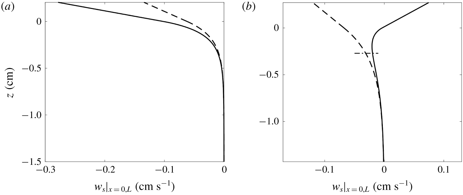
The streaming flow velocity distribution along the lateral boundary when  $a_{0}=0.2g_{0}$,
 $f_{0}=8~\text{Hz}$ for (a) the symmetric and (b) the antisymmetric cases. The solid line is the result (3.27) with the sum terminated at
 $m+n=200$, while the dashed line contains contributions from the gravest mode only. The upper limit of the plot is the position of the liquid surface at hydrophilic boundary. The dash-dotted line in (b) shows the liquid surface position at the hydrophobic boundary.

The vertical velocity distribution near the lateral boundary is shown in figure 9. The contribution from the gravest mode is similar in both the symmetric and antisymmetric cases. The two cases become distinct once higher-order contributions are included. The streaming velocity becomes stronger, but remains monotonic and negative in the symmetric case. In the antisymmetric case, the higher-order contributions weaken the streaming velocity and create a profile that is positive above  $z=0.013~\text{cm}$ and has a negative extremum approximately 0.2 cm below the surface. This effect is due to phase modulation within the harmonic spectrum,
 $A_{n}$. All the
 $A_{n}$ are positive in the symmetric case, so the components add constructively. In the antisymmetric case,
 $A_{1}$ is negative and the other
 $A_{n}$ are positive, so interactions between the gravest and higher-order modes interfere destructively with the contributions from the wave self-interactions. Thus, in contrast to the monochromatic wave situation discussed by Périnet et al. (Reference Périnet, Gutiérrez, Urra, Mujica and Gordillo2017), the lateral boundary streaming velocity profile is affected by the relative phases of the component waves. In this experiment, the relative phases are controlled by the symmetry of static meniscus. Note that the streaming velocity is left–right symmetric in the symmetric case, but asymmetric in the antisymmetric case because the free surface on the hydrophobic side is lower than that on the hydrophilic side (see figure 9b).
3.2.3 Numerical simulation of streaming circulation
Following Périnet et al. (Reference Périnet, Gutiérrez, Urra, Mujica and Gordillo2017), we obtain the secondary flow in the bulk by using the steady streaming velocity profile as boundary conditions for the laminar flow solver in COMSOL Multiphysics® using a fixed (i.e. not deforming) domain at  $\unicode[STIX]{x1D711}=\unicode[STIX]{x03C0}$. Taking the characteristic velocity
 $U$ to be the r.m.s. velocity of the surface streaming velocity distribution, and the characteristic length to be the cell width
 $L$, the maximum Reynolds number is 24 for streaming circulation. We simulate the steady secondary circulation at seven different oscillation amplitudes with the driving frequency
 $f_{0}=8~\text{Hz}$.
The secondary flow velocity beneath the oscillating meniscus for the symmetric case from (a) the numerical simulation and (b) the experiment. The forcing amplitude is  $a_{0}=0.2g_{0}$ and the driving frequency is
 $f_{0}=8~\text{Hz}$. The phase chosen for simulation is
 $\unicode[STIX]{x1D711}=\unicode[STIX]{x03C0}$. The centre of the anticlockwise (clockwise) circulation is denoted by
 $E_{acw}$ (
 $E_{cw}$). The point where the velocity perpendicular to the line connecting
 $E_{acw}$ and
 $E_{cw}$ is maximal, denoting a transition between anticlockwise and clockwise vortices, is given by
 $T$.

The secondary flow velocity beneath the oscillating meniscus for the antisymmetric case from (a) the numerical simulation and (b) the experiment. The forcing amplitude is  $a_{0}=0.2g_{0}$ and the driving frequency is
 $f_{0}=8~\text{Hz}$. The phase chosen for simulation is
 $\unicode[STIX]{x1D711}=\unicode[STIX]{x03C0}$. The centre of the anticlockwise (clockwise) circulation is denoted by
 $E_{acw}$ (
 $E_{cw}$). The point where the velocity perpendicular to the line connecting
 $E_{acw}$ and
 $E_{cw}$ is maximal, denoting a transition between anticlockwise and clockwise vortices, is given by
 $T$.

The steady secondary circulation induced by the oscillation at  $a_{0}=0.2g_{0}$ is shown in figures 10 and 11. A nonlinear transformation is applied to the magnitude of the flow vectors to better visualize their direction. The numerical simulation successfully reproduces the four-vortex circulation structure in the symmetric case and the dipole circulation structure in the antisymmetric case. The scalings for the r.m.s. speed,
 $v_{rms}$, and the symmetry parameter,
 $\unicode[STIX]{x1D6FE}$, from the numerical simulations are shown in figure 5. The numerical solutions follow the same scaling law,
 $v_{rms}\sim (a_{0}/g_{0})^{2}$, as the experiments, but the value of the r.m.s. speed is approximately one order of magnitude smaller (figure 5a). The error in the first-order solution (see figure 7) accounts for approximately 15 % of the total error in both symmetric and antisymmetric cases; the remaining error must be due to other effects.
In order to determine the source of this additional error, we quantify the rotation speed of the eddies to gain additional insight into the streaming circulation structure and the energy distribution in the bulk. The rotation speed of each vortex is measured along a section connecting the centre of a anticlockwise circulation,  $E_{acw}$, and the adjacent clockwise circulation,
 $E_{cw}$. The two vortices are separated by the point
 $T$ where the velocity perpendicular to
 $E_{acw}E_{cw}$ is maximal. The radii and speed of the vortices are then defined by
 $$\begin{eqnarray}r_{acw}=\unicode[STIX]{x0394}(E_{acw}T),\quad v_{acw}=\frac{1}{r_{acw}}\int _{E_{acw}\rightarrow T}v_{n}\,\text{d}l,\end{eqnarray}$$
 $$\begin{eqnarray}r_{cw}=\unicode[STIX]{x0394}(E_{cw}T),\quad v_{cw}=\frac{1}{r_{cw}}\int _{T\rightarrow E_{cw}}v_{n}\,\text{d}l,\end{eqnarray}$$
where  $\unicode[STIX]{x0394}(E_{acw}T)$ and
 $\unicode[STIX]{x0394}(E_{cw}T)$ are the lengths of the lines connecting
 $E_{acw}$ and
 $E_{cw}$, respectively, to
 $T$, and
 $v_{n}$ is the velocity perpendicular to
 $E_{acw}E_{cw}$. The resulting speed and radii for the different cases are shown in table 1.
Radii and speed for vortices from the simulations and experiments.

We find that  $r_{cw}$ is always smaller than
 $r_{acw}$, while
 $v_{cw}$ is always larger than
 $v_{acw}$. This means that the vortices near the hydrophilic boundary are smaller and relatively faster in both the symmetric and antisymmetric cases. The speed of the vortices is of the order
 $10^{-3}{-}10^{-2}~\text{cm}~\text{s}^{-1}$ for both the experiments and simulations. Consistent with the result from the
 $v_{rms}$ calculation, the experiment gives a result approximately five or six times larger than the simulation. The difference between simulation and experiment is slightly larger for the clockwise vortex than for the anticlockwise vortex. This suggests that our model fails to completely capture the physics of the hydrophilic boundary. The impact of three-dimensional (3-D) effects on the circulation is estimated in appendix A by calculating the compression rate. We find a significant secondary flow convergence in the
 $y$ direction near the hydrophilic boundary (figure 12). The convergence near the hydrophilic boundary induces a downwelling jet on the observational plane and makes a significant contribution to the secondary circulation near the hydrophilic boundary. This effect explains the significant symmetry loss in the antisymmetric case and may account for the remaining discrepancy between the simulations and experiments.
The numerical experiments were repeated with the surface streaming condition replaced by a free-slip boundary. The four-vortex structure is lost in the symmetric case and the kinetic energy drops by an order of magnitude in both cases. These results demonstrate that the free surface is a significant source of momentum for the secondary circulation and is important for determining its qualitative structure.
Divergence of the 2-D streaming flow at  $a_{0}/g_{0}=0.2$ and
 $f_{0}=8~\text{Hz}$ for (a) the symmetric and (b) the antisymmetric cases. Negative contours are dashed. The phase
 $\unicode[STIX]{x1D711}=9/10\unicode[STIX]{x03C0}$ (
 $\unicode[STIX]{x1D711}=13/10\unicode[STIX]{x03C0}$) for the symmetric (antisymmetric) case.

4 Conclusion
We observe the streaming circulation excited by standing capillary–gravity waves using PIV. It is found that the structure of the streaming circulation is controlled by the static meniscus shape. A semi-analytical theory is developed which explains the streaming pattern.
The experiment is designed to inhibit Faraday waves, so the streaming circulation is driven by meniscus waves, rather than by Faraday waves, as reported previously (Gordillo & Mujica Reference Gordillo and Mujica2014; Périnet et al. Reference Périnet, Gutiérrez, Urra, Mujica and Gordillo2017). Two different linear meniscus wave modes in the  $x$ direction are generated by choosing the boundary wettability conditions. In experiments with hydrophilic–hydrophilic boundary conditions, the static meniscus is symmetric and the gravest meniscus wave mode has two nodes. In experiments with hydrophobic–hydrophilic boundary conditions, however, the static meniscus is antisymmetric and the gravest mode has a single node. The experimentally measured free-surface profiles are used to develop an analytical model for the linear meniscus waves. This model reveals that meniscus waves are standing capillary–gravity waves with a spectrum determined by the Fourier spectrum of the static meniscus profile. The analytical results give the correct dominant mode number and structure, and predict the wave amplitude within an order of magnitude of the experimental results.
The secondary circulation induced by the meniscus wave is observed by broadcasting PIV images stroboscopically. The secondary flow originates from the Stokes boundary layer under a contaminated free surface, where the Reynolds stress induced by the meniscus wave is balanced by the viscous stress. The meniscus wave produces a four-vortex structure in the symmetric case, while a vortex dipole is generated in the antisymmetric case. The r.m.s. circulation speed,  $v_{rms}$, scales like the square of the forcing amplitude (i.e.
 $v_{rms}\sim (a_{0}/g_{0})^{2}$), regardless of the static surface profile. For
 $a_{0}=0.2g_{0}$, the secondary circulation has a speed of
 $10^{-3}{-}10^{-2}~\text{cm}~\text{s}^{-1}$. In the symmetric case, the secondary flow retains a high degree of left–right symmetry as the forcing amplitude is increased. For the antisymmetric case, the flow symmetry is broken; such an asymmetry comes from the exponential decay of the velocity from
 $z=0$, so the places with higher mean elevation have greater velocity under them. As a result, the antisymmetric surface profile gives rise to the asymmetry of streaming circulation.
Using the strategy suggested by Nicolás & Vega (Reference Nicolás and Vega2003) and Gordillo & Mujica (Reference Gordillo and Mujica2014), we simulate the secondary flow by calculating the streaming velocities along the free surface and lateral boundaries and use these as boundary conditions for a laminar model. The simulated secondary flows have the same spatial structures, obey the same speed scaling, and have similar symmetry properties as the experimental flows. The theoretical model reveals that the secondary flow is shaped by the entire wave spectrum rather than by a monochromatic wave, as has been studied extensively in the previous literature. In particular, the relative phases of harmonic modes significantly affect the resulting streaming velocity distribution.
Several limitations of this analysis should be re-emphasized. First, although the theory successfully captures the spatial structure of the meniscus wave, the solution is inaccurate in the region near the contact line because we have assumed that the surface slope is small, whereas  $\unicode[STIX]{x2202}_{x}\unicode[STIX]{x1D701}\sim 1$ near the contact line. Furthermore, the physics of the contact line and dynamic contact angle at microscopic scales were not considered (c.f. Yi, Ding & Spelt Reference Yi, Ding and Spelt2014). Second, the theory focuses on 2-D dynamics, since the experiment only measures a single cross-section of the flow field. However, 3-D effects play some role in the secondary circulation, but we lack the data to fully account for these effects. For these reasons, the agreement between the theory and experiment is not fully quantitative. In particular, the amplitudes of the meniscus waves and the strengths of the secondary circulations are underestimated. Based on the limitations of the present study, the streaming circulation inside the wedge in the vicinity of the contact line would be an interesting point for further research.
Acknowledgements
We are grateful to J. Yu, R. Wilson and D.-P. Wang for stimulating discussions. We also thank J.-Q. Shi and Z. Chen for their participation in the early stage of the experiment. This work was supported by the National Science Foundation of China through grant nos 11572230 and 11772235, and a NSFC/RGC Joint Grant no. 11561161004.
Declaration of interests
The authors report no conflict of interest.
Supplementary movies
Supplementary movies that show the streaming circulations produced by an oscillating meniscus (symmetric/antisymmetric,  $a_{0}=0.2g_{0}$,
 $f_{0}=8~\text{Hz}$) are available at https://doi.org/10.1017/jfm.2020.281.
Appendix A. Estimates of 3-D effects
To estimate how motion in the  $y$ direction affects the motion in the
 $x$–
 $z$ plane, we compute the 2-D divergence rate, defined as
 $$\begin{eqnarray}\unicode[STIX]{x2202}_{x}u+\unicode[STIX]{x2202}_{z}w.\end{eqnarray}$$
The hydrophilic boundaries are regions of strong divergence, while the hydrophobic boundary is associated with less intense, but larger-scale, convergence (figure 12). In the symmetric case, the divergence zones are flanked by weaker convergence zones, which indicate flow in the plane directed away from the boundaries (i.e. from the divergence to the convergence zones). The arrangement of convergence and divergence zones in the antisymmetric case implies a more broadly distributed flow from the right (hydrophilic) boundary to the left (hydrophobic) boundary. The divergent flow contributes to the streaming circulation in both cases and enhances the asymmetry of the antisymmetric case. Since our experiment only imaged in midplane of the fluid cell, we lack the data to determine the cause of this 3-D circulation. Further experiments and 3-D analysis should be designed to examine this 3-D secondary flow.
Appendix B. Faraday threshold
This experiment focuses on streaming driven by natural cavity standing wave modes, rather than a Faraday wave excited by parametric instability. The experiment is therefore conducted in a stable zone of the Faraday instability. Here, we demonstrate that the experiment is indeed within a stable zone. The time-dependent surface deformation,  $\unicode[STIX]{x1D701}_{kl}$, of a linear standing wave mode in a rectangular channel is
 $$\begin{eqnarray}\displaystyle \unicode[STIX]{x1D701}_{kl}=a_{kl}(t)\cos \left(\frac{\unicode[STIX]{x03C0}kx}{L_{x}}\right)\cos \left(\frac{\unicode[STIX]{x03C0}ly}{L_{y}}\right), & & \displaystyle\end{eqnarray}$$
where  $(k,l)$ are the mode numbers in the
 $x$ and
 $y$ directions, respectively, and
 $a_{kl}$ is the mode amplitude. From Benjamin & Ursell (Reference Benjamin and Ursell1954), the mode amplitude
 $a_{kl}$ evolves according to the differential equation
 $$\begin{eqnarray}\displaystyle \frac{\text{d}^{2}a_{kl}}{\text{d}T^{2}}+[p_{kl}-2q_{kl}\cos (2T)]a_{kl}=0, & & \displaystyle\end{eqnarray}$$
which is known as Mathieu’s equation (Abramowitz & Stegun Reference Abramowitz and Stegun1965). In this equation,  $T={\textstyle \frac{1}{2}}\unicode[STIX]{x1D714}t$ is dimensionless time and the parameters
 $p_{kl}$ and
 $q_{kl}$ are
 $$\begin{eqnarray}\displaystyle & \displaystyle p_{kl}=\frac{4K_{kl}\tanh (K_{kl}h)}{\unicode[STIX]{x1D714}^{2}}\left(g_{0}+\frac{\unicode[STIX]{x1D70E}}{\unicode[STIX]{x1D70C}}K_{kl}^{2}\right), & \displaystyle\end{eqnarray}$$
 $$\begin{eqnarray}\displaystyle & \displaystyle q_{kl}=2K_{kl}a_{0}\frac{\tanh (K_{kl}h)}{\unicode[STIX]{x1D714}^{2}}, & \displaystyle\end{eqnarray}$$
where
 $$\begin{eqnarray}K_{kl}^{2}=\frac{\unicode[STIX]{x03C0}^{2}k^{2}}{L_{x}^{2}}+\frac{\unicode[STIX]{x03C0}^{2}l^{2}}{L_{y}^{2}}\end{eqnarray}$$
is the total wavenumber. The mathematical character of Mathieu’s equation is such that some modes grow exponentially in time while others – in the stable zones – decay exponentially. The decaying modes are not observable in this experiment, since their amplitudes rapidly become too small to measure. For the forcing frequency  $f_{0}=8~\text{Hz}$,
 $$\begin{eqnarray}\displaystyle p_{10}\approx 2.5,\quad p_{20}\approx 7.1, & & \displaystyle \nonumber\end{eqnarray}$$
and the associated instability thresholds are  $q_{10}^{T}\approx 2.6$ and
 $q_{20}^{T}\approx 4.4$ (Abramowitz & Stegun Reference Abramowitz and Stegun1965). The corresponding threshold forcing accelerations are
 $a_{10}^{T}\approx 2.36g_{0}$ and
 $a_{20}^{T}\approx 2.01g_{0}$. In our experiment, we chose
 $a_{0}\leqslant 0.36g_{0}$, which is well below the Faraday instability threshold and the observed
 $(1,0)$ and
 $(2,0)$ modes are therefore ordinary resonant modes.
Appendix C. Extrapolation method
In this section, we describe the extrapolation method used to calculate the streaming velocity distribution along the meniscus at  $z=\unicode[STIX]{x1D701}_{0}(x)$. Instead of extrapolating the secondary flow velocity directly, we extrapolate the primary flow (i.e. the linear meniscus wave) velocity to ensure continuity of the first-order velocity. The primary flow velocities extrapolated to the static meniscus are
 $$\begin{eqnarray}\displaystyle & \displaystyle u_{1}|_{z=\unicode[STIX]{x1D701}_{0}}\approx \left.u_{1}|_{z=0}+\frac{\unicode[STIX]{x2202}u_{1}}{\unicode[STIX]{x2202}z}\right|_{z=0}\unicode[STIX]{x1D701}_{0}=-\cos \unicode[STIX]{x1D714}t\,\mathop{\sum }_{n}^{\infty }A_{n}k_{n}[1+k_{n}\unicode[STIX]{x1D701}_{0}]\sin k_{n}x, & \displaystyle\end{eqnarray}$$
 $$\begin{eqnarray}\displaystyle & \displaystyle w_{1}|_{z=\unicode[STIX]{x1D701}_{0}}\approx \left.w_{1}|_{z=0}+\frac{\unicode[STIX]{x2202}w_{1}}{\unicode[STIX]{x2202}z}\right|_{z=0}\unicode[STIX]{x1D701}_{0}=\cos \unicode[STIX]{x1D714}t\,\mathop{\sum }_{n}^{\infty }A_{n}k_{n}[1+k_{n}\unicode[STIX]{x1D701}_{0}]\cos k_{n}x. & \displaystyle\end{eqnarray}$$
The velocity tangent to the free surface is the projection of (C 1) and (C 2) onto the tangential direction  $\hat{\boldsymbol{t}}$:
 $$\begin{eqnarray}\displaystyle u_{\Vert } & = & \displaystyle (u_{1},w_{1})|_{z=\unicode[STIX]{x1D701}_{0}}\boldsymbol{\cdot }\hat{\boldsymbol{t}}\nonumber\\ \displaystyle & = & \displaystyle -\cos \unicode[STIX]{x1D714}t\,\mathop{\sum }_{n}^{\infty }A_{n}k_{n}\frac{1+k_{n}\unicode[STIX]{x1D701}_{0}}{[1+(\unicode[STIX]{x2202}_{x}\unicode[STIX]{x1D701}_{0})^{2}]^{1/2}}(\sin k_{n}x-\unicode[STIX]{x2202}_{x}\unicode[STIX]{x1D701}_{0}\cos k_{n}x)\nonumber\\ \displaystyle & {\approx} & \displaystyle -\cos \unicode[STIX]{x1D714}t\,\mathop{\sum }_{n}^{\infty }A_{n}k_{n}(1+k_{n}\unicode[STIX]{x1D701}_{0})\sin k_{n}x,\end{eqnarray}$$
where we have used the fact that  $\unicode[STIX]{x2202}_{x}\unicode[STIX]{x1D701}_{0}\sim O(\unicode[STIX]{x1D716})$ in the last step. Again using the fact that
 $\unicode[STIX]{x2202}_{x}\unicode[STIX]{x1D701}_{0}\sim O(\unicode[STIX]{x1D716})$, we estimate the tangential derivative of the tangential velocity as
 $$\begin{eqnarray}\unicode[STIX]{x2202}_{\unicode[STIX]{x1D70F}}u_{\Vert }\approx \unicode[STIX]{x2202}_{x}u_{\Vert }\approx \cos \unicode[STIX]{x1D714}t\,\mathop{\sum }_{n}^{\infty }A_{n}k_{n}(1+k_{n}\unicode[STIX]{x1D701}_{0})(\unicode[STIX]{x2202}_{xx}^{2}\unicode[STIX]{x1D701}_{0}-k_{n})\cos k_{n}x.\end{eqnarray}$$
Substituting (C 3) and (C 4) into (3.23), we find that the streaming velocity along the free surface is

where we have used the facts that  , and
 . The process is similar for extrapolation on the lateral boundaries. When
 $z\leqslant 0$, the streaming velocity is the same as for a flat surface. When
 $z>0$, the vertical velocity at arbitrary position
 $z^{\prime }$ is estimated by
 $$\begin{eqnarray}w_{1}|_{z=z^{\prime }}\approx w_{1}|_{z=0}+\left.\frac{\unicode[STIX]{x2202}w_{1}}{\unicode[STIX]{x2202}z}\right|_{z=0}z^{\prime }.\end{eqnarray}$$
It should be mentioned that the extrapolation for the velocity does not converge for arbitrary order of the Taylor expansion. As  $A_{n}$ converges like
 $n^{-5}$, the extrapolation polynomial in (C 1) and (C 2) should be no higher than the second order.
Appendix D. Derivation of the boundary layer streaming velocity
In this section, we provide a detailed derivation of a 2-D boundary layer streaming velocity under a vibrating solid boundary with a curved unperturbed state, i.e. equations (3.23) and (3.24), using the method of Nicolás & Vega (Reference Nicolás and Vega2003). The derivation in this appendix uses dimensionless variables to maintain consistency with Nicolás & Vega (Reference Nicolás and Vega2003). The duplicated symbols  $t$,
 $\unicode[STIX]{x1D70F}$,
 $f$,
 $U$ and
 $F$ share the same physical meaning as those in the rest of the paper, but do not have units. The tangential oscillation of the boundary is not considered in this derivation.
D.1 Governing equation
We scale lengths by the capillary length  $l_{c}$, velocity by
 $\unicode[STIX]{x1D714}l_{c}$ and pressure by
 $\unicode[STIX]{x1D70C}\unicode[STIX]{x1D714}^{2}l_{c}^{2}$. The non-dimensional 2-D Navier–Stokes and continuity equations transformed into a curvilinear orthogonal coordinate frame,
 $(\unicode[STIX]{x1D70F},\unicode[STIX]{x1D709})$, following the unperturbed boundary are
 $$\begin{eqnarray}\displaystyle & \unicode[STIX]{x2202}_{t}\tilde{v}+\tilde{v}\unicode[STIX]{x2202}_{\unicode[STIX]{x1D70F}}\tilde{v}+\tilde{w}\unicode[STIX]{x2202}_{\unicode[STIX]{x1D709}}\tilde{v}-\tilde{w}\unicode[STIX]{x1D705}\tilde{v}=-(1+\unicode[STIX]{x1D709}\unicode[STIX]{x1D705})\unicode[STIX]{x2202}_{\unicode[STIX]{x1D70F}}p+R^{-1}\unicode[STIX]{x2202}_{\unicode[STIX]{x1D709}\unicode[STIX]{x1D709}}^{2}\tilde{v}, & \displaystyle\end{eqnarray}$$
 $$\begin{eqnarray}\displaystyle & \unicode[STIX]{x2202}_{t}\tilde{w}+\tilde{v}\unicode[STIX]{x2202}_{\unicode[STIX]{x1D70F}}\tilde{w}+\tilde{w}\unicode[STIX]{x2202}_{\unicode[STIX]{x1D709}}\tilde{w}+\tilde{v}\unicode[STIX]{x1D705}\tilde{v}=-\unicode[STIX]{x2202}_{\unicode[STIX]{x1D709}}p+R^{-1}\unicode[STIX]{x2202}_{\unicode[STIX]{x1D709}\unicode[STIX]{x1D709}}^{2}\tilde{w}, & \displaystyle\end{eqnarray}$$
 $$\begin{eqnarray}\displaystyle & \unicode[STIX]{x2202}_{\unicode[STIX]{x1D70F}}\tilde{v}+\unicode[STIX]{x2202}_{\unicode[STIX]{x1D709}}\tilde{w}-\unicode[STIX]{x1D705}\tilde{w}=0, & \displaystyle\end{eqnarray}$$
where the velocity in curvilinear coordinates is denoted by  $(\tilde{u} ,\tilde{v})$ and
 $R$ is the Reynolds number, defined by
 $R=\unicode[STIX]{x1D714}l_{c}^{2}/\unicode[STIX]{x1D708}$. The small parameter used for the asymptotic expansion is
 $\unicode[STIX]{x1D716}=a_{0}/(\unicode[STIX]{x1D714}^{2}l_{c})$. The basic asymptotic assumptions of Nicolás & Vega (Reference Nicolás and Vega2003), namely that
 $R\gg 1$ and
 $\unicode[STIX]{x1D716}\ll 1$, are satisfied by our experiments.
To study the boundary layer flow inside the oscillatory boundary layer, equations (D 1)–(D 3) are further rescaled by
 $$\begin{eqnarray}\unicode[STIX]{x1D70F}^{\ast }=\unicode[STIX]{x1D70F},\quad \tilde{w}^{\ast }=\tilde{w}-\unicode[STIX]{x2202}_{t}\,f-\tilde{v}\unicode[STIX]{x2202}_{\unicode[STIX]{x1D70F}}f,\quad \unicode[STIX]{x1D702}=R^{1/2}(\unicode[STIX]{x1D709}-f).\end{eqnarray}$$
The boundary layer thickness is  $O(R^{-1/2})$, the tangential velocity
 $\tilde{v}$ and surface deformation
 $f$ are
 $O(\unicode[STIX]{x1D716})$, and the normal velocity
 $\tilde{w}$ is
 $O(\unicode[STIX]{x1D716}R^{-1/2}+\unicode[STIX]{x1D716}^{2})$. Eliminating terms smaller than
 $O(\unicode[STIX]{x1D716}R^{-1/2}+\unicode[STIX]{x1D716}^{2})$, the equations for a boundary layer on an oscillating solid boundary are
 $$\begin{eqnarray}\unicode[STIX]{x2202}_{t}\tilde{v}+\tilde{v}\unicode[STIX]{x2202}_{\unicode[STIX]{x1D70F}}\tilde{v}+R^{1/2}[(\tilde{w}^{\ast }+\tilde{v}\unicode[STIX]{x2202}_{\unicode[STIX]{x1D70F}}f)\unicode[STIX]{x2202}_{\unicode[STIX]{x1D702}}\tilde{v}-\unicode[STIX]{x2202}_{\unicode[STIX]{x1D702}}p\unicode[STIX]{x2202}_{\unicode[STIX]{x1D70F}}f]-\unicode[STIX]{x1D705}\unicode[STIX]{x2202}_{t}\,f\tilde{v}+\unicode[STIX]{x2202}_{\unicode[STIX]{x1D70F}}p+(f+R^{-1/2}\unicode[STIX]{x1D702})\unicode[STIX]{x1D705}\unicode[STIX]{x2202}_{\unicode[STIX]{x1D70F}}p-\unicode[STIX]{x2202}_{\unicode[STIX]{x1D702}\unicode[STIX]{x1D702}}^{2}\tilde{v}=0,\end{eqnarray}$$
 $$\begin{eqnarray}\displaystyle & \unicode[STIX]{x2202}_{\unicode[STIX]{x1D702}}p+R^{-1/2}(\unicode[STIX]{x2202}_{tt}^{2}f-\unicode[STIX]{x2202}_{\unicode[STIX]{x1D702}\unicode[STIX]{x1D702}}^{2}\tilde{w}^{\ast })=0, & \displaystyle\end{eqnarray}$$
 $$\begin{eqnarray}\displaystyle & \unicode[STIX]{x2202}_{\unicode[STIX]{x1D702}}\tilde{w}^{\ast }+R^{-1/2}(\unicode[STIX]{x2202}_{\unicode[STIX]{x1D70F}}\tilde{v}-\unicode[STIX]{x1D705}\unicode[STIX]{x2202}_{t}\,f)=0. & \displaystyle\end{eqnarray}$$
These are identical to the 2-D form of equations (5.1)–(5.4) in Nicolás & Vega (Reference Nicolás and Vega2003). For notational convenience, we drop the  $^{\ast }$ decorating
 $t^{\ast }$ and
 $\unicode[STIX]{x1D70F}^{\ast }$ in (D 5)–(D 7). The boundary condition at
 $\unicode[STIX]{x1D702}=0$ is
 $$\begin{eqnarray}\displaystyle \tilde{w}^{\ast }=0,\quad \tilde{v}=0. & & \displaystyle\end{eqnarray}$$
The connection condition at  $\unicode[STIX]{x1D702}\rightarrow \infty$ depends on the form of the equation at each scale.
D.2 Perturbation solution
Consider the perturbation expansion
 $$\begin{eqnarray}\displaystyle & f=\unicode[STIX]{x1D716}F\text{e}^{\text{i}t}+\text{c.c.}+\cdots \,, & \displaystyle\end{eqnarray}$$
 $$\begin{eqnarray}\displaystyle & \tilde{v}=\unicode[STIX]{x1D716}(V_{0}+R^{-1/2}V_{1})\text{e}^{\text{i}t}+\text{c.c.}+\unicode[STIX]{x1D716}^{2}(v^{s}+\text{O.T.})+\cdots \,, & \displaystyle\end{eqnarray}$$
 $$\begin{eqnarray}\displaystyle & \tilde{w}^{\ast }=\unicode[STIX]{x1D716}R^{-1/2}W_{1}\text{e}^{\text{i}t}+\text{c.c.}+\unicode[STIX]{x1D716}^{2}(w^{s}+\text{O.T.})+\cdots \,, & \displaystyle\end{eqnarray}$$
 $$\begin{eqnarray}\displaystyle & p=\unicode[STIX]{x1D716}(P_{0}+R^{-1/2}P_{1})\text{e}^{\text{i}t}+\text{c.c.}+\unicode[STIX]{x1D716}^{2}(p^{s}+\text{O.T.})+\cdots \,. & \displaystyle\end{eqnarray}$$
Here  $F$ is the deformation amplitude perpendicular to the liquid surface,
 $V$ and
 $W$ are the tangential and normal velocity amplitudes, respectively, and
 $P$ is the pressure amplitude. The numbers in the subscripts represent the order number. The time-independent streaming components of the tangential velocity, normal velocity and pressure are
 $v^{s}$,
 $w^{s}$ and
 $p^{s}$, respectively; and O.T. stands for oscillation terms with zero average. We substitute these expansions into (D 5)–(D 7) and solve at order
 $O(\unicode[STIX]{x1D716})$,
 $O(\unicode[STIX]{x1D716}/\sqrt{R})$ and
 $O(\unicode[STIX]{x1D716}^{2})$ sequentially.
The solution at  $O(\unicode[STIX]{x1D716})$ order represents a typical Stokes boundary layer:
 $$\begin{eqnarray}\displaystyle & P_{0}=P_{0}^{0}(\unicode[STIX]{x1D70F}), & \displaystyle\end{eqnarray}$$
 $$\begin{eqnarray}\displaystyle & V_{0}=U(\unicode[STIX]{x1D70F})(1-\text{e}^{\sqrt{\text{i}}\unicode[STIX]{x1D702}}), & \displaystyle\end{eqnarray}$$
where we take the branch of the square root where  $\sqrt{\text{i}}=-(1+\text{i})/\sqrt{2}$. The pressure gradient along the free surface is balanced by the outer (potential) flow acceleration, so we have
 $$\begin{eqnarray}\displaystyle \unicode[STIX]{x2202}_{\unicode[STIX]{x1D70F}}P_{0}^{0}=-\text{i}U, & & \displaystyle\end{eqnarray}$$
where  $U$ is the outer flow amplitude. The connection condition is
 $\unicode[STIX]{x2202}_{\unicode[STIX]{x1D702}}V_{0}|_{\unicode[STIX]{x1D702}\rightarrow \infty }=0$.
At order  $O(\unicode[STIX]{x1D716}/\sqrt{R})$, the solution is
 $$\begin{eqnarray}\displaystyle & \displaystyle P_{1}=F\unicode[STIX]{x1D702}+P_{1}^{0}(\unicode[STIX]{x1D70F}), & \displaystyle\end{eqnarray}$$
 $$\begin{eqnarray}\displaystyle & \displaystyle V_{1}=-\text{i}\unicode[STIX]{x2202}_{\unicode[STIX]{x1D70F}}P_{1}^{0}(1+\text{e}^{\sqrt{\text{i}}\unicode[STIX]{x1D702}})+H\unicode[STIX]{x1D702}, & \displaystyle\end{eqnarray}$$
 $$\begin{eqnarray}\displaystyle & \displaystyle W_{1}=(\text{i}\unicode[STIX]{x1D705}F-\unicode[STIX]{x2202}_{\unicode[STIX]{x1D70F}}U)\unicode[STIX]{x1D702}+(\text{e}^{\sqrt{\text{i}}\unicode[STIX]{x1D702}}-1)\frac{\unicode[STIX]{x2202}_{\unicode[STIX]{x1D70F}}U}{\sqrt{\text{i}}}, & \displaystyle\end{eqnarray}$$
where  $H=\unicode[STIX]{x1D705}U+\text{i}\unicode[STIX]{x2202}_{\unicode[STIX]{x1D70F}}F$ and
 $P_{1}^{0}(\unicode[STIX]{x1D70F})$ is an arbitrary function.
At order  $O(\unicode[STIX]{x1D716}^{2})$, the streaming pressure
 $p^{s}$ and normal velocity
 $w^{s}$ are
 $$\begin{eqnarray}\displaystyle & p^{s}=p^{s0}(\unicode[STIX]{x1D70F}), & \displaystyle\end{eqnarray}$$
 $$\begin{eqnarray}\displaystyle & w^{s}=0, & \displaystyle\end{eqnarray}$$
where  $p^{s0}(\unicode[STIX]{x1D70F})$ is also an arbitrary function to be determined. The horizontal streaming velocity can be integrated under the condition
 $\unicode[STIX]{x2202}_{\unicode[STIX]{x1D702}}v^{s}|_{\unicode[STIX]{x1D702}\rightarrow \infty }=0$ and has the limit at
 $\unicode[STIX]{x1D702}\rightarrow \infty$ of
 $$\begin{eqnarray}\displaystyle v^{s}|_{\unicode[STIX]{x1D702}\rightarrow \infty }=3\unicode[STIX]{x1D705}F^{\ast }U-{\textstyle \frac{3}{2}}[U\unicode[STIX]{x2202}_{\unicode[STIX]{x1D70F}}U^{\ast }+\text{i}U\unicode[STIX]{x2202}_{\unicode[STIX]{x1D70F}}U^{\ast }]+\text{c.c.} & & \displaystyle\end{eqnarray}$$
This results in the boundary layer flow at  $\unicode[STIX]{x1D702}\rightarrow \infty$ and holds for the outer flow at the unperturbed boundary at
 $\unicode[STIX]{x1D709}=f$. The streaming pressure
 $p^{s}$ is chosen to cancel the singularity in the integration of
 $v^{s}$ and is
 $$\begin{eqnarray}\displaystyle p^{s}=|F|^{2}-|U|^{2}+p^{s0}, & & \displaystyle\end{eqnarray}$$
where  $p^{s0}$ is independent of
 $\unicode[STIX]{x1D702}$ or
 $\unicode[STIX]{x1D70F}$.
D.3 Streaming velocity at the unperturbed boundary
Since the solution (D 21) is only valid at  $\unicode[STIX]{x1D709}=f$, we must extrapolate the result onto the unperturbed boundary at
 $\unicode[STIX]{x1D709}=0$ during the numerical simulation. A first-order Taylor expansion from
 $\unicode[STIX]{x1D709}=f$ gives
 $$\begin{eqnarray}\displaystyle & \tilde{v}(\unicode[STIX]{x1D709})=\tilde{v}|_{\unicode[STIX]{x1D709}=f}+\unicode[STIX]{x2202}_{\unicode[STIX]{x1D709}}\tilde{v}|_{\unicode[STIX]{x1D709}=f}(\unicode[STIX]{x1D709}-f)+\cdots \,, & \displaystyle\end{eqnarray}$$
 $$\begin{eqnarray}\displaystyle & \tilde{w}(\unicode[STIX]{x1D709})=\tilde{w}|_{\unicode[STIX]{x1D709}=f}+\unicode[STIX]{x2202}_{\unicode[STIX]{x1D709}}\tilde{w}|_{\unicode[STIX]{x1D709}=f}(\unicode[STIX]{x1D709}-f)+\cdots \,. & \displaystyle\end{eqnarray}$$
The matching condition is that the outer flow should be consistent with the boundary layer flow at  $R\rightarrow \infty$ and
 $\unicode[STIX]{x1D702}\rightarrow \infty$, so we have
 $$\begin{eqnarray}f=\unicode[STIX]{x1D716}F\text{e}^{\text{i}t}+\text{c.c.}+\cdots \,,\end{eqnarray}$$
 $$\begin{eqnarray}\displaystyle \tilde{v} & = & \displaystyle \unicode[STIX]{x1D716}V_{0}|_{\unicode[STIX]{x1D702}\rightarrow \infty }\text{e}^{\text{i}t}+\text{c.c.}+\unicode[STIX]{x1D716}^{2}(v^{s}|_{\unicode[STIX]{x1D702}\rightarrow \infty }+\text{O.T.})+\cdots \nonumber\\ \displaystyle & = & \displaystyle \unicode[STIX]{x1D716}U\text{e}^{\text{i}t}+\text{c.c.}+\unicode[STIX]{x1D716}^{2}(v^{s}|_{\unicode[STIX]{x1D709}=f}+\text{O.T.})+\cdots \,,\end{eqnarray}$$
 $$\begin{eqnarray}\displaystyle \tilde{w} & = & \displaystyle \unicode[STIX]{x2202}_{t}\,f+\tilde{v}\unicode[STIX]{x2202}_{\unicode[STIX]{x1D70F}}f+\cdots \nonumber\\ \displaystyle & = & \displaystyle \unicode[STIX]{x1D716}\text{i}F\text{e}^{\text{i}t}+\text{c.c.}+\unicode[STIX]{x1D716}^{2}(U\unicode[STIX]{x2202}_{\unicode[STIX]{x1D70F}}F^{\ast }+\text{c.c.}+\text{O.T.})+\cdots \nonumber\\ \displaystyle & = & \displaystyle \unicode[STIX]{x1D716}\text{i}F\text{e}^{\text{i}t}+\text{c.c.}+\unicode[STIX]{x1D716}^{2}(w^{s}|_{\unicode[STIX]{x1D709}=f}+\text{O.T.})+\cdots \,.\end{eqnarray}$$
Using the expansion  $\unicode[STIX]{x2202}_{\unicode[STIX]{x1D709}}\tilde{v}=\unicode[STIX]{x1D705}\tilde{v}+\unicode[STIX]{x2202}_{\unicode[STIX]{x1D70F}}\tilde{w}$, and the continuity equation
 $\unicode[STIX]{x2202}_{\unicode[STIX]{x1D70F}}\tilde{v}+\unicode[STIX]{x2202}_{\unicode[STIX]{x1D709}}\tilde{w}-\unicode[STIX]{x1D705}\tilde{w}=0$, we find
 $$\begin{eqnarray}\displaystyle & \unicode[STIX]{x2202}_{\unicode[STIX]{x1D709}}\tilde{v}=\unicode[STIX]{x1D716}[(\unicode[STIX]{x1D705}U+\text{i}\unicode[STIX]{x2202}_{\unicode[STIX]{x1D70F}}F)\text{e}^{\text{i}t}+\text{c.c.}]+\cdots \,, & \displaystyle\end{eqnarray}$$
 $$\begin{eqnarray}\displaystyle & \unicode[STIX]{x2202}_{\unicode[STIX]{x1D709}}\tilde{w}=\unicode[STIX]{x1D716}[(\text{i}\unicode[STIX]{x1D705}F-\unicode[STIX]{x2202}_{\unicode[STIX]{x1D70F}}U)\text{e}^{\text{i}t}+\text{c.c.}]+\cdots \,. & \displaystyle\end{eqnarray}$$
Substituting (D 21) and (D 25)–(D 29) into (D 23) and (D 24) and averaging over an oscillation period results in
 $$\begin{eqnarray}\displaystyle v^{s}|_{\unicode[STIX]{x1D709}=0} & = & \displaystyle v^{s}|_{\unicode[STIX]{x1D702}\rightarrow \infty }-\overline{\unicode[STIX]{x2202}_{\unicode[STIX]{x1D709}}|_{\unicode[STIX]{x1D709}=f}\tilde{v}f}\nonumber\\ \displaystyle & = & \displaystyle \left[3\unicode[STIX]{x1D705}F^{\ast }U-{\textstyle \frac{3}{2}}(U\unicode[STIX]{x2202}_{\unicode[STIX]{x1D70F}}U^{\ast }+\text{i}U\unicode[STIX]{x2202}_{\unicode[STIX]{x1D70F}}U^{\ast })\right]-(\unicode[STIX]{x1D705}F^{\ast }U+\text{i}F^{\ast }\unicode[STIX]{x2202}_{\unicode[STIX]{x1D70F}}F)+\text{c.c.}\nonumber\\ \displaystyle & = & \displaystyle 2\unicode[STIX]{x1D705}F^{\ast }U-{\textstyle \frac{3}{2}}(U\unicode[STIX]{x2202}_{\unicode[STIX]{x1D70F}}U^{\ast }+\text{i}U\unicode[STIX]{x2202}_{\unicode[STIX]{x1D70F}}U^{\ast })-\text{i}F^{\ast }\unicode[STIX]{x2202}_{\unicode[STIX]{x1D70F}}F+\text{c.c.}\end{eqnarray}$$
and
 $$\begin{eqnarray}\displaystyle w^{s}|_{\unicode[STIX]{x1D709}=0} & = & \displaystyle w^{s}|_{\unicode[STIX]{x1D702}\rightarrow \infty }-\overline{\unicode[STIX]{x2202}_{\unicode[STIX]{x1D709}}|_{\unicode[STIX]{x1D709}=f}\tilde{w}f}\nonumber\\ \displaystyle & = & \displaystyle U\unicode[STIX]{x2202}_{\unicode[STIX]{x1D70F}}F^{\ast }+F^{\ast }\unicode[STIX]{x2202}_{\unicode[STIX]{x1D70F}}U-\text{i}\unicode[STIX]{x1D705}F^{\ast }F+\text{c.c.}\nonumber\\ \displaystyle & = & \displaystyle \unicode[STIX]{x2202}_{\unicode[STIX]{x1D70F}}(UF^{\ast })+\text{c.c.},\end{eqnarray}$$
where an overbar denotes a time average. Equations (D 30) and (D 31) are 2-D versions of equations (6.2) and (6.3) in Nicolás & Vega (Reference Nicolás and Vega2003).