1. Introduction
Social infrastructures, including plant facilities, bridges, and tunnels, are essential to the public. However, infrastructure deterioration due to long-term use poses significant challenges. Rebuilding such structures is expensive and time-consuming. Therefore, proper maintenance is crucial. To prevent building deterioration, inspections are conducted using scaffolding [1] and special cranes [Reference Sharp2]. However, these inspections incur enormous costs, pose the danger of working at great heights, and faces a shortage of inspectors.
To address existing problems, various robots have been developed. Such robots are classified into flying [Reference Metani and Hamel3–Reference Rosales, Gandolfo, Scaglia, Jordan and Carelli11], adhesive [Reference Song, Wang, Wang, Ji and Zhu12–Reference Parween, Tan and Elara22], and wire robots [Reference Fujisawa, Umemoto, Tanaka, Sato, Nagatani and Katsuyama23, Reference Ishida, Hirose and Guarnieri24]. A magnetic wheel robot (a type of adhesion robot) easily performs contact inspection because the robot is always in contact with steel structures. Additionally, robots can perform inspections for a long time because they do not consume electricity when not in use. However, the robots must travel along complex three-dimensional (3D) paths. The most difficult route in complex 3D paths is the one that moves from the bottom to the top surface of a flange.
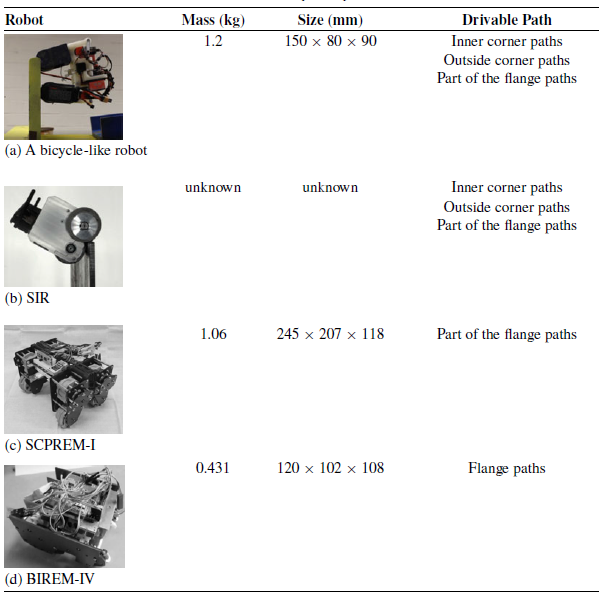
Robots developed in previous studies.

Few wheeled robots are designed to travel along a flange section. Examples of robots capable of traveling along a flange section are shown in Table I.
-
a. A bicycle-like robot [Reference Nguyen, La and La25] features a variable wheelbase to traverse a flange section.
-
b. SIR [Reference Zürich26] has short wheelbase.
Therefore, these robots can traverse the flange if the direction of the flange’s protrusion is compatible with their design. However, the references don’t mention a path from the bottom to the top surface of a flange.
The robots that can travel along path from the bottom to the top surface of a flange are shown in (c) and (d). Reference [Reference Tanida, Ono, Kobayashi, Shiba and Takada27] mentions that it is difficult to travel along the flange path due to gravity and counter torques of the motors.
(c) SCPREM-I [Reference Tanida, Ono, Kobayashi, Shiba and Takada27] not only changes wheelbase but also use counter-torque with planetary gear mechanism.
(d) BIREM-IV [Reference Kawamoto, Matsumura and Takada28] achieved traversal by combining a short wheelbase with a lightweight design. Nevertheless, the traversal success rate remains low: approximately 30% for (c) and 10% for (d). Therefore, it is possible that when inspection equipment is mounted on the robots, these robots cannot travel due to increase in mass.
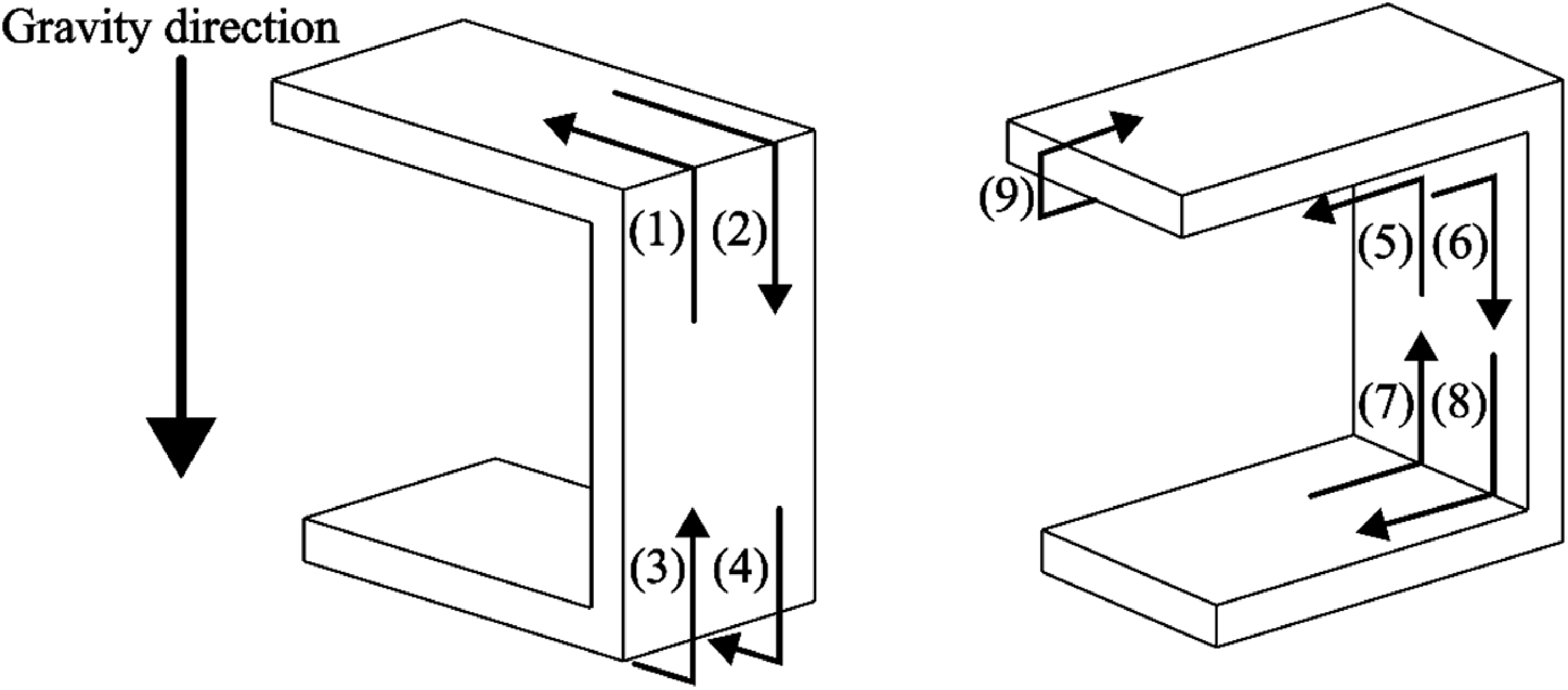
Through static analysis, we confirmed that the effects of gravity and counter torques when a robot traverses a flange path can be mitigated by changing its posture. To achieve this, we developed a robot equipped with a pushing mechanism to adjust its posture. Experimental results demonstrated that this mechanism effectively facilitates traversal along flange paths. Additionally, a weight was attached to the robot, and running experiments were conducted. It was confirmed that the robot could successfully travel along all paths in Figure 1, including outside corner paths (1)–(4), inner corner paths (5)–(8), and flange path (9), and that the robot has sufficient expandability to mount inspection equipment.
Three-dimensional paths.

2. Analysis Running Along the Flange Path
2.1. Issues with running along the flange path
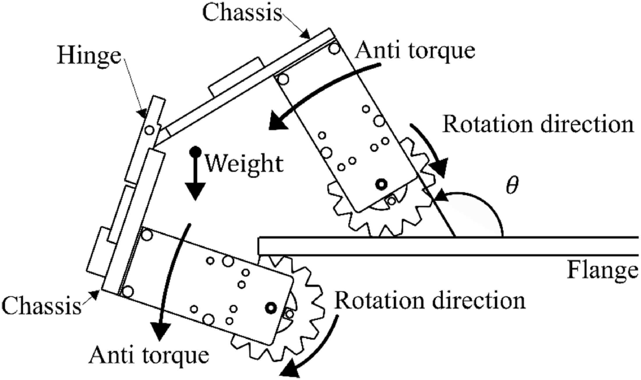
Figure 2 shows the diagram of a robot moving from the underside to the top side of a flange. The front and rear wheels adhere to the top and underside of the flange, respectively. Furthermore, the front and rear chassis are connected using a hinge. When these motors rotate the wheels clockwise, the robot attempts to move towards the top of the flange. However, gravity and counterclockwise anti-torque act on the robot. Gravity and anti-torque affect the robot chassis as counterclockwise moments of force. Owing to the moment of force pushing down on the robot, traveling from the underside to the top side of the flange becomes difficult.
Forces and anti-torques that impede flange travel.

2.2. Changes in the effects of gravity and counter-torque depending on the robot’s posture
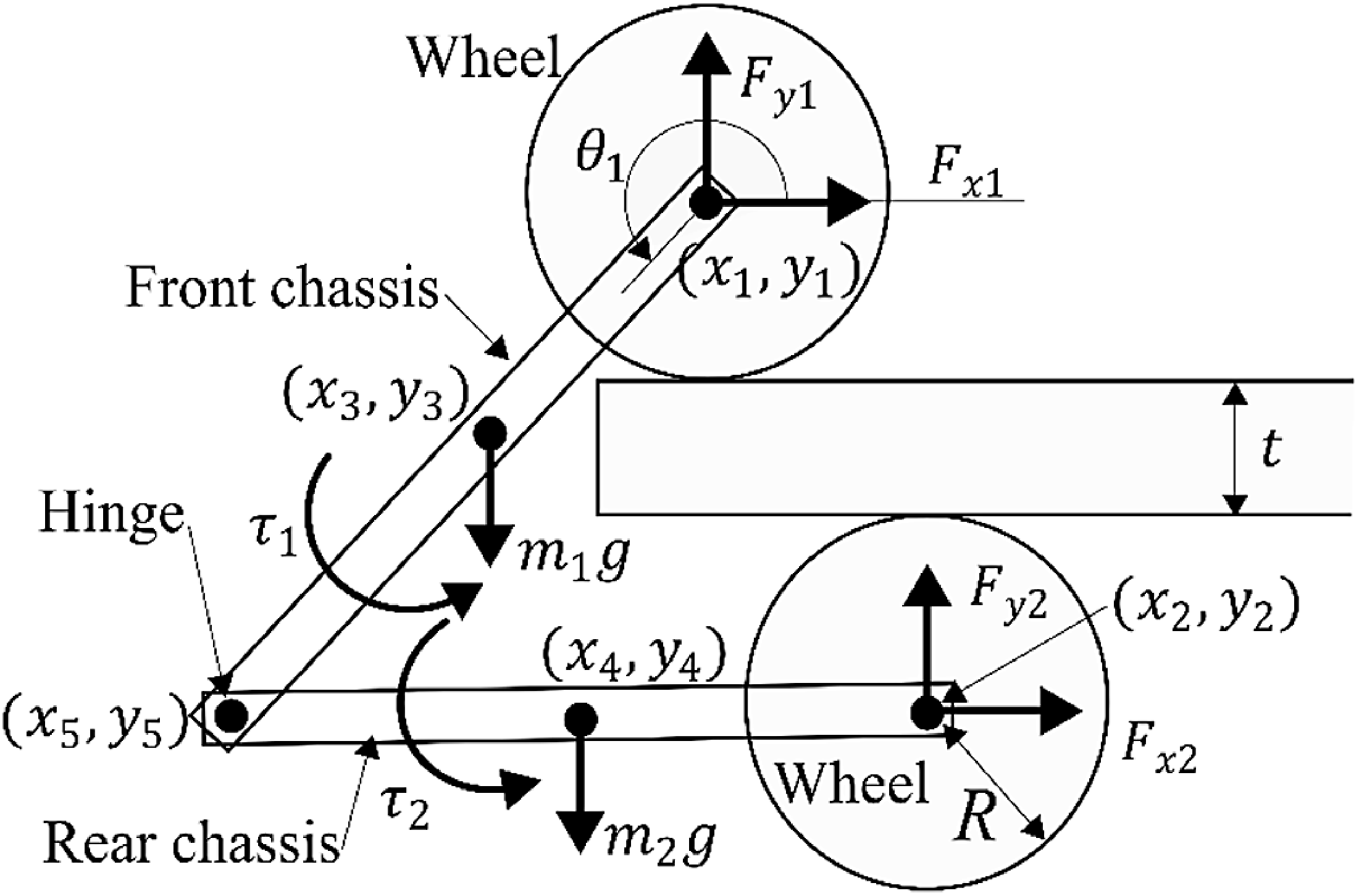
Figure 3 shows the schematic of a simple magnetic wheel robot model moving from the underside to the top side of a flange. Herein,
 $\theta _{1}$
is the angle of the front chassis relative to the top surface of the flange. Traversing the path is difficult because the robot is pushed down by gravity and anti-torque. However, the effects can be reduced depending on the value of
 $\theta _{1}$
. Therefore, using a simple model, the force that the wheels receive from the riding surface when stationary is calculated based on
 $\theta _{1}$
. The model comprises two front wheels, two rear wheels, a front chassis, and a rear chassis. The front and rear chassis are connected using a hinge. Herein,
 $(x_{1},y_{1})$
and
 $(x_{2},y_{2})$
represent the central position of the front and rear wheels, respectively;
 $(x_{3},y_{3})$
and
 $(x_{4},y_{4})$
locate the center of gravity of the front and rear chassis, respectively; and
 $(x_{5},y_{5})$
represents the hinge position. Further,
 $m_{1}$
and
 $m_{2}$
denote the mass of the front and rear chassis, respectively;
 $F_{x1}$
and
 $F_{y1}$
represent the forces on the front chassis from the front wheels;
 $F_{x2}$
and
 $F_{y2}$
denote the forces on the rear chassis from the rear wheels; and
 $\tau _{1}$
and
 $\tau _{2}$
denote the counter torques of the motor that drive the front and rear wheels, respectively.
Force and anti-torque acting on the chassis.

Initially, we only consider the equation of balance for the chassis. Subsequently, forces from the wheels are calculated when the chassis is stationary. As the front and rear chassis are connected by hinges, the force balance equations [Eqs. (1) and (2)], and moment of force balance equations [Eqs. (3) and (4)] are established.
The horizontal force balance equation is expressed as
 \begin{equation} F_{x1}+F_{x2}=0 \end{equation}
The vertical force balance equation is expressed as
 \begin{equation} F_{y1}+F_{y2}-\left(m_{1}+m_{2}\right)g=0 \end{equation}
The moment of force balance around the center of the front wheel is expressed as
 \begin{eqnarray} 2\tau _{1} + 2\tau _{2}+F_{x2}\left(y_{1}-y_{2}\right)+F_{y2}\left(x_{2}-x_{1}\right) -\, m_{1}g\left(x_{3}-x_{1}\right)-m_{2}g\left(x_{4}-x_{1}\right)=0 \end{eqnarray}
The moment of force balance around the hinge at the rear chassis is expressed as
 \begin{equation} 2\tau _{2}+F_{x2}\left(y_{5}-y_{2}\right)+F_{y2}\left(x_{2}-x_{5}\right)-m_{2}g\left(x_{4}\, -x_{5}\right)=0 \end{equation}
By solving the four simultaneous equations, the forces
 $F_{x1}$
,
 $F_{y1}$
,
 $F_{x2}$
, and
 $F_{y2}$
can be determined. Further, using the wheel-force balance equations, we determine the forces exerted on the wheels by the riding surface. The forces acting on the wheels are illustrated in Figure 4, where
 $m_{3}$
and
 $m_{4}$
denote the mass of the front and rear wheels, respectively;
 $F_{wx1}$
and
 $F_{wy1}$
represent the forces of the front wheels acting on the riding surface;
 $F_{wx2}$
and
 $F_{wy2}$
represent the forces of the rear wheels acting on the riding surface; and
 $F_{\textrm{mag}}$
denotes the adhesive force of the wheel to the riding surface. Notably, two front and two rear wheels are considered. Thus,
 $F_{wx1}$
,
 $F_{wy1}$
,
 $F_{wx2}$
, and
 $F_{wy2}$
are calculated from the horizontal and vertical force balance equations as
Force exerted on the wheels.

 \begin{align} F_{wx1} &=\frac{F_{x1}}{2} \end{align}
 \begin{align} F_{wy1} &=F_{\textrm{mag}}+\frac{F_{y1}}{2}+m_{3}g \end{align}
 \begin{align} F_{wx2} &=\frac{F_{x2}}{2} \end{align}
 \begin{align} F_{wy2} &=-F_{\textrm{mag}}+\frac{F_{y2}}{2}+m_{4}g \end{align}
Force and coefficient of friction required to remain stationary according to
 $\theta _{1}$
.

The forces
 $F_{wx1}$
,
 $F_{wy1}$
,
 $F_{wx2}$
, and
 $F_{wy2}$
are determined for
 $\theta _{1}$
, as shown in Figure 5(a). Additionally, the static friction coefficient between the front wheel and the riding surface (
 $\mu _{w1}$
) and that between the rear wheel and the riding surface (
 $\mu _{w2}$
) required for static conditions are shown in Figure 5(b). Herein,
 $\mu _{w1}$
and
 $\mu _{w2}$
are defined as
 \begin{align} \mu _{w1} &=\frac{F_{wx1}}{F_{wy1}} \end{align}
 \begin{align} \mu _{w2} &=\frac{F_{wx2}}{F_{wy2}} \end{align}
In Figure 5, the values of
 $F_{wx1}$
,
 $F_{wx2}$
,
 $\mu _{w1}$
, and
 $\mu _{w2}$
peak when
 $\theta _{1}$
is near 180° to 190°. Reducing
 $\theta _{1}$
to less than 180° decreases the required driving force and friction coefficient for the robot to remain stationary. Therefore, a mechanism to lift the chassis of the robot for controlling
 $\theta _{1}$
is adopted. Furthermore, the driving force and friction coefficient required for running decrease on reducing
 $\theta _{1}$
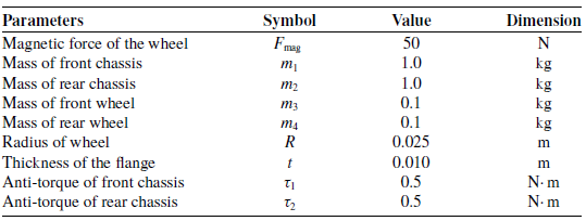
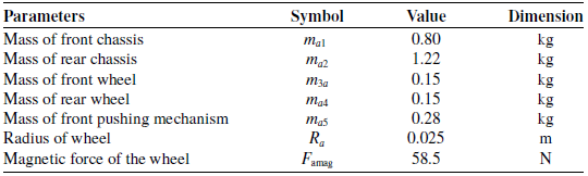
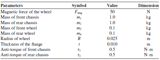
, allowing the robot to run on the flange section. The parameters used for the calculations are shown in Table II.
Parameters used for calculations.
Photographs of the magnetic wheel robot.

3. Methodology
3.1. Overview of the magnet wheel robot
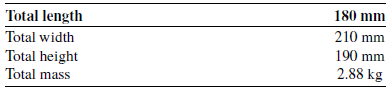
The robot developed for flange running was improved by referencing robots designed in previous studies [Reference Nakajima, Shiba and Takada29, Reference Kobayashi, Nakajima, Shiba, Song and Takada30]. The developed robot is shown in Figure 6. The robot specifications are listed in Table III. The robot uses a four-wheel drive system, with each wheel driven by its own geared motor. The motor torque constant is 0.011 N· m/A and the reduction ratio of the decelerator is 370:1. The viscous friction torque
 $\tau$
(N· m), with
 $\dot{\theta }_{m}$
representing the motor’s rotational speed (rad/s), is given by the equation
 $\tau \,=\, 4.71\times 10^{-7}\dot{\theta }_{m}\, +\, 1.77\times 10^{-4}$
. The efficiency, which is independent of the rotational speed, was experimentally determined to be 0.67. The geared motor and wheel intersect at a right angle, and motor power is transmitted to the wheel via miter gears. When the robot travels along a flange path, the wheelbase must be adjusted according to the thickness of the flange. Therefore, the front and rear chassis are connected using a hinge. Additionally, pushing mechanisms to traverse inner corner and flange paths are attached to the front and rear chassis. Furthermore, inertial measurement unit (IMU) sensors are attached to the front chassis, rear chassis, and front pushing mechanism for the robot posture recognition. The parts of the robot that require strength are designed using chopped carbon-containing nylon resin sheets, aluminum alloy, and stainless steel. Additionally, the parts that do not require strength are fabricated using acrylic board.
Specifications of the magnetic wheel robot.

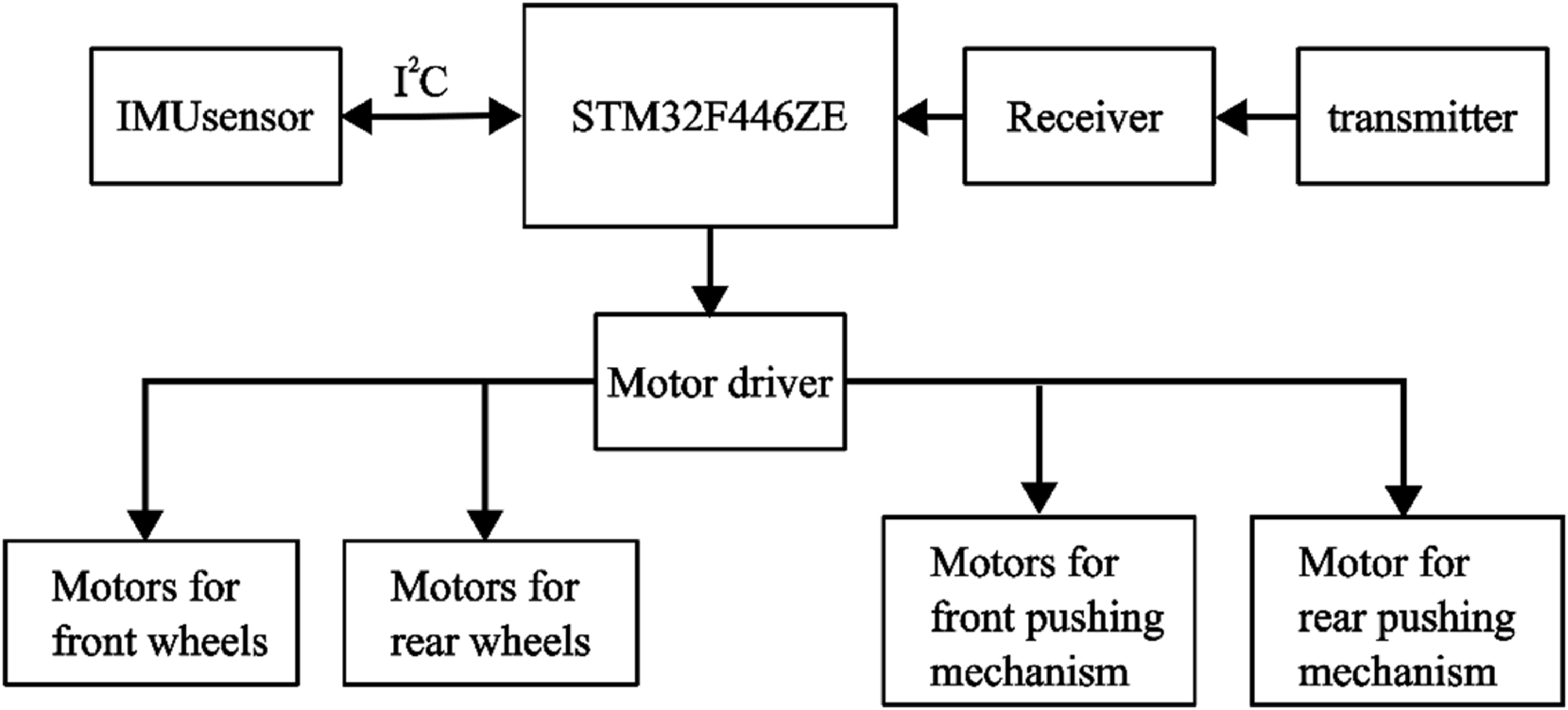
The robot system is shown in Figure 7. The STM32F446ZE board receives a signal from the receiver and sends a corresponding PWM signal to the motor driver. Therefore, motors are controlled via PWM. Also, the signal from the receiver can be manually changed by operating the transmitter. Additionally, information about the robot’s posture is obtained using IMU sensors connected to the STM32F446ZE board via I2C communication.
Robot system.

3.2. Magnetic wheel
The magnetic wheel structure of the robot and the yoke shape of the wheel are shown in Figures 8(a) and (b). As shown in Figure 8(a), the magnetic wheel comprises two iron yokes (ss400) and two ring magnets, with the magnets sandwiched between the yokes. Moreover, as shown in Figure 8(b), the iron yoke is concave and convex shaped with outer and inner diameters of 50 and 24 mm, respectively. When the wheels are circular, as shown in Figure 9(a), they can slip at the corners, making movement difficult. Therefore, by constructing uneven wheels, corners are caught, as shown in Figure 9(b), thereby allowing the robot to move without slipping.
Magnetic wheel.

Comparison of wheel shape.

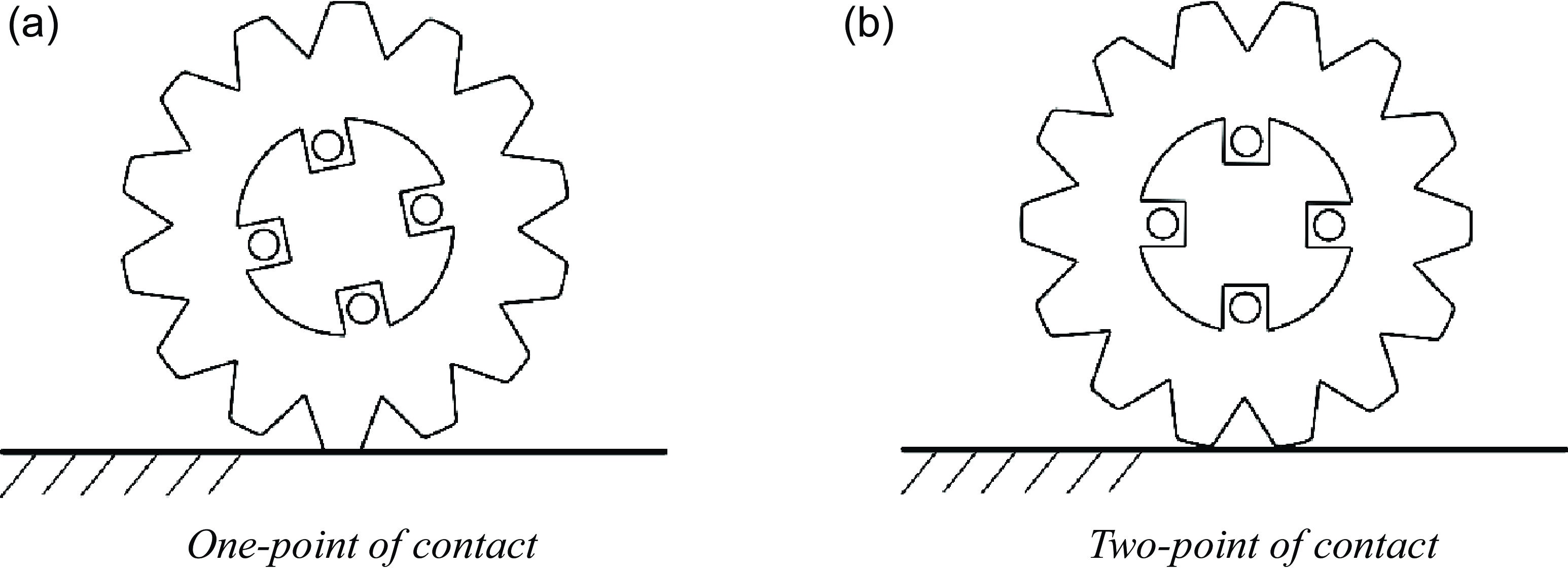
The adhesive force and static friction coefficient of the wheels relative to a steel plate were calculated using an FGP-50 digital force gauge manufactured by NIDEC Drive Technology Corporation. As all four wheels of the robot are fabricated using the same material and method, only one of them was measured. To measure the adhesive force, the magnetic wheel was pulled vertically from a steel plate. The maximum pulling force required to detach the wheel from the steel surface was measured. Additionally, the magnetic wheel was pulled horizontally onto the steel plate to measure the static friction coefficient. Subsequently, the maximum pulling force required to move the wheel was measured. The static friction coefficient was calculated by dividing the maximum pulling force by the adhesive force. Each measurement was performed five times, and the averages were considered the adhesive force and static friction coefficient. As the wheels were uneven, they adhered to one or two points, as shown in Figures 10(a) and (b). The adhesive force and the static friction coefficient varied depending on how the wheels adhered; therefore, the two patterns were measured. Additionally, the steel that was used in the running flange during the experiment was used as the experimental environment. The results are shown in Table IV.
From the results, it was confirmed that even if the adsorption force is reduced due to one-point contact, sufficient adsorption and static friction forces can be obtained when adhering to a ceiling or wall. These forces are adequate to support the gravitational force (2.88 × 9.81 = 28.3 n) acting on the robot through its four wheels.
Specifications of the magnetic wheel.

Contact pattern of the wheel.

3.3. Motor and decelerator
The magnetic wheel receives strong resistance from a steel surface. Therefore, high torque is required to drive the wheel. Considering only the magnetic force, when the wheel is in two-point contact, the maximum static friction torque can be calculated as 0.52 N· m, based on Table IV and the wheel radius of 0.025 m. Therefore, a geared motor is used to output high torque, and an experiment was conducted to evaluate its ability to drive the wheel.
A pulley with a diameter of 60 mm was attached to the output shaft of the geared motor. When a voltage of 9.0 V was applied, the motor successfully lifted a 3.0 kg weight, corresponding to a load of 0.88 N· m. This confirmed that the geared motor could generate sufficient torque to overcome static friction and drive the wheels on a flat surface.
3.4. Front pushing mechanism
To change the posture of the robot while moving through the flange sections, a pushing mechanism developed in a previous study was adopted [Reference Matsumura, Shiba, Ito, Kawase and Takada31]. Additionally, when the robot moved through an inner corner and the front wheels adhered to both the floor and wall, strong adhesion prevented the wheels from rotating. Consequently, the robot became immobile. Therefore, the mechanism enabled the robot to move by pressing the floor with a push rod and lifting the wheels off the adhesive surface.
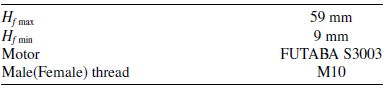
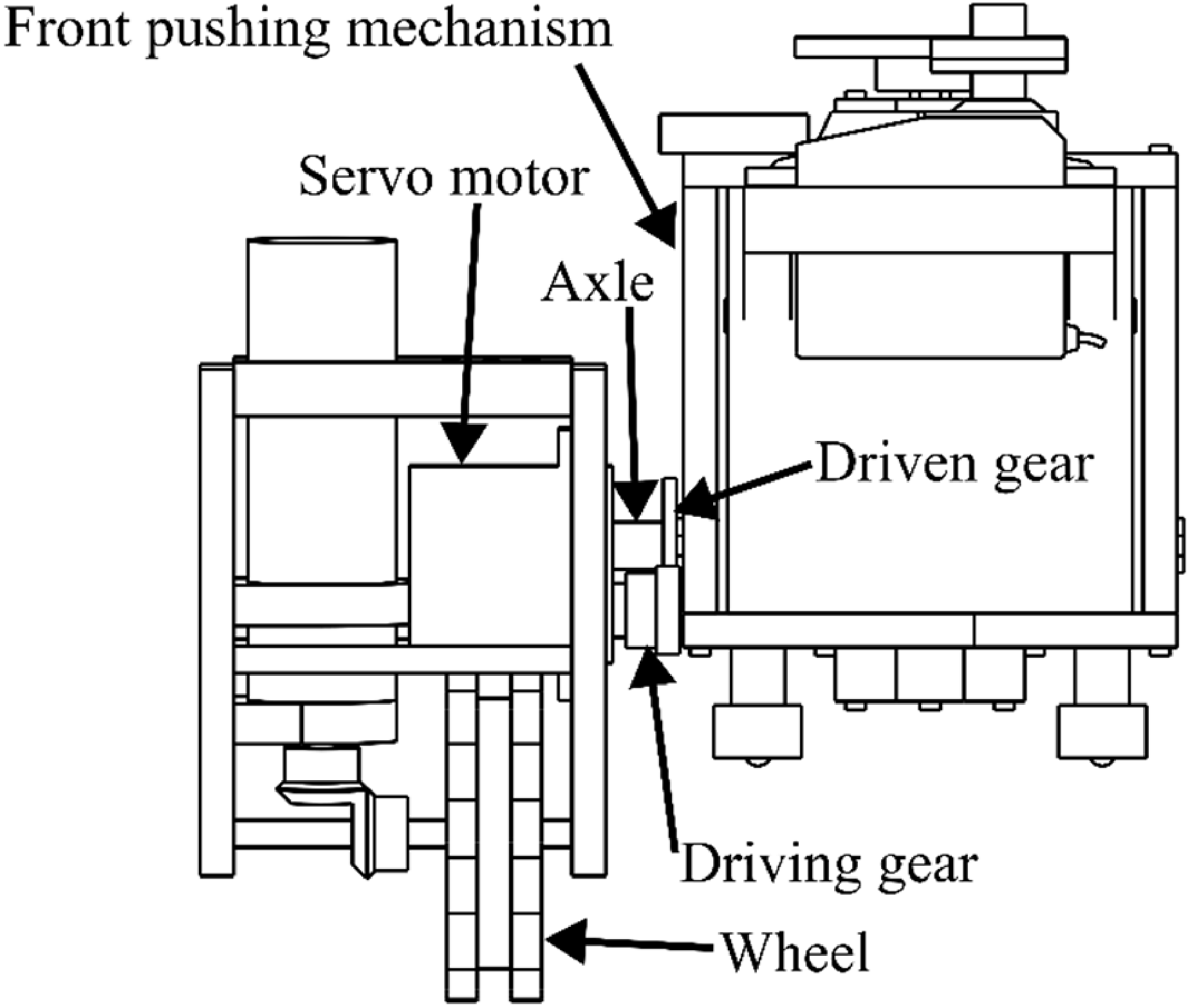
The front pushing mechanism is shown in Figures 11(a) and (b), while the mounting positions are shown in Figure 11(c). The specifications are listed in Table V. Herein,
 $H_{f}$
indicates the extension length of the push rods. The mechanism primarily comprised a servo motor (Futaba S3003), which was modified for continuous rotation, driving gear (module 0.5, 80 teeth), driven gear (module 0.5, 40 teeth), trapezoidal screw thread, female trapezoidal screw thread, and push rods. Additionally, ball bearings were attached to the tips of the push rods. When the motor was driven, the trapezoidal screw thread rotated, and the trapezoidal female screw thread moved linearly. Therefore, the push rods attached to the trapezoidal female screw thread were pressed on the riding surface.
Specifications of the front pushing mechanism.

Front pushing mechanism.

The front pushing mechanism (right side) and the rotating mechanism (left side) are shown in Figure 12. The pushing mechanism was attached to the front chassis by inserting an axle into the radial bearing shown in Figure 11(b). Additionally, when the servo motor (GWServo Micro 2BBMG), in Figure 12, was driven, the driving force was transmitted to the pushing mechanism via the driving gear (module 0.5, 25 teeth) and the driven gear (module 0.5, 42 teeth). Thus, the angle of the pushing mechanism was adjusted relative to that of the front chassis.
Rotation mechanism.

Using the mechanism, the robot was lifted from the start of extrusion [Figure 13(a)] through the intermediate stage in Figure 13(b) to the completion of extrusion in Figure 13(c), while keeping the pushing mechanism vertical and pressing the rod against the floor.
Upward pushing mechanism of the robot.

Rear pushing mechanism.

3.5. Rear pushing mechanism
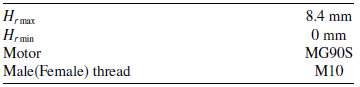
When the robot moved through an inner corner and the rear wheels adhered to both the floor and wall, strong adhesion prevented the wheels from rotating. Consequently, the robot became immobile. Therefore, a pushing mechanism different from that discussed in Section 3.4 was attached to the rear chassis. The rear pushing mechanism is shown in Figures 14(a) and 14(b). The mounting position is shown in Figure 14(c), and the specifications are listed in Table VI. Herein,
 $H_{r}$
denotes the extension lengths of the push rods. The mechanism was similar to the front pushing mechanism described in Section 3.4. Therefore, when the motor was driven, the push rods were pressed against the riding surface. The motor is Tower Pro MG90S, which was modified for continuous rotation. The driving gear is module 0.5 and 10 teeth, and the driven gear is module 0.5 and 80 teeth.
Specifications of the rear pushing mechanism.

3.6. Consideration of flange running
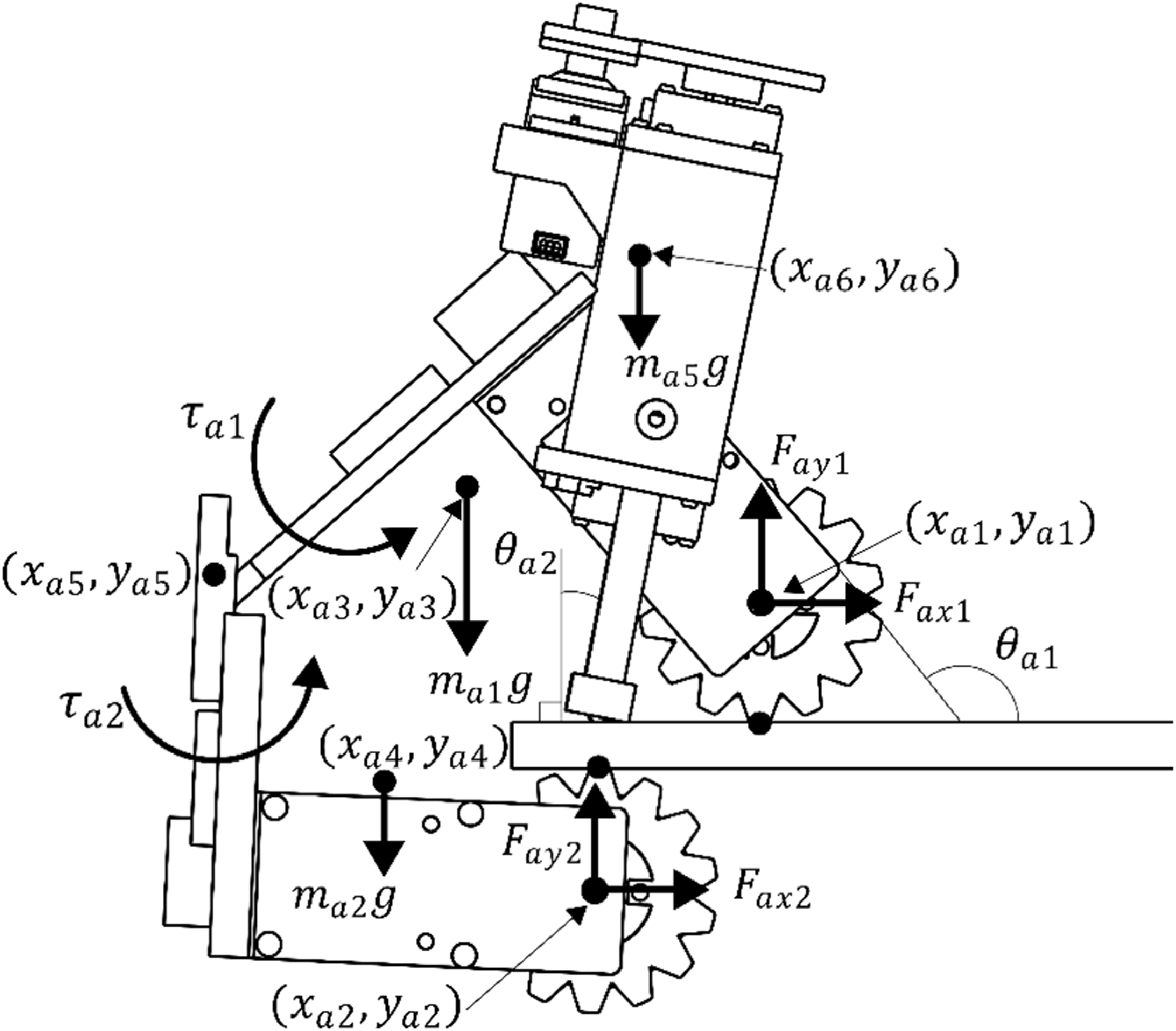
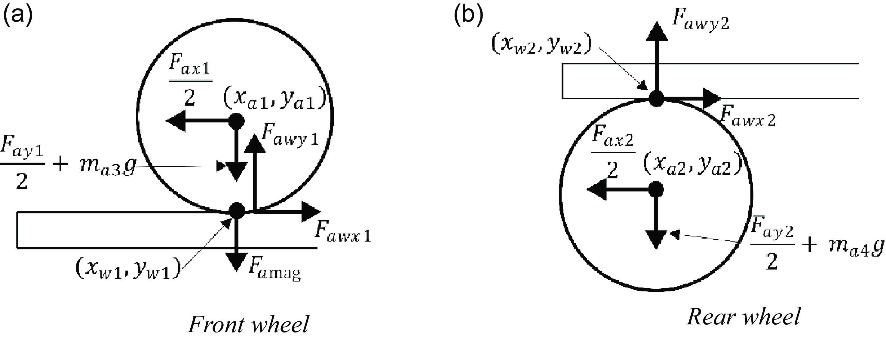
The static running conditions from the underside to the top of the flange (Path 9) were calculated. When the robot traveled along Path 9, the front pushing mechanism was used to lift its body, as shown in Figure 15. In addition, the robot moved forward and transitioned toward the top of the flange. Therefore, calculations were performed based on the situation shown in Figure 15. The most challenging situation for the robot is when it is no longer supported by the push rods. Therefore, static analysis is conducted under the condition where the push rods are not in contact with the running surface. The calculation method was the same as that used for the simplified model described in Section 2.2.
Force and torque applying the chassis.

The forces and torques acting on the chassis are illustrated in Figure 15. Herein,
 $(x_{a1},y_{a1})$
and
 $(x_{a2},y_{a2})$
denote the center position of the front and rear wheels, respectively;
 $(x_{a3},y_{a3})$
and
 $(x_{a4},y_{a4})$
represent the center of gravity of the front chassis and rear chassis combined with the rear pushing mechanism, respectively;
 $(x_{a5},y_{a5})$
represents the hinge position;
 $(x_{a6},y_{a6})$
is the center of gravity of the pushing mechanism;
 $\theta _{a1}$
is the angle between the front chassis and the upper surface of the flange; and
 $\theta _{a2}$
is the angle between the front pushing mechanism and the upper surface of the flange. Additionally,
 $m_{a1}$
and
 $m_{a2}$
denote the mass of the front chassis and the combined mass of the rear chassis and the rear pushing mechanism, respectively;
 $m_{a5}$
is the mass of the front pushing mechanism;
 $F_{ax1}$
and
 $F_{ay1}$
are the forces exerted on the front chassis by the front wheel;
 $F_{ax2}$
and
 $F_{ay2}$
as the forces exerted on the rear chassis by the rear wheel; and
 $\tau _{a1}$
and
 $\tau _{a2}$
are the counter-torque of the motor driving the front and rear wheels, respectively. Additionally, as a condition, the minimum value of
 $\theta _{a1}$
was set to
 $113^{\circ}$
, and
 $\theta _{a2}$
was fixed at
 $10^{\circ}$
.
As the front and rear chassis were connected by hinges, the force balance equations [Eqs. (11) and (12)] and the moment of force balance equations [Eqs. (13) and (14)] were calculated.
The horizontal force balance equation is expressed as
 \begin{equation} F_{ax1}+F_{ax2}=0 \end{equation}
The vertical force balance equation is expressed as
 \begin{equation} F_{ay1}+F_{ay2}-\left(m_{a1}+m_{a2}+m_{a5}\right)g=0 \end{equation}
The moment of force balance around the center of the front wheel is expressed as
 \begin{eqnarray} 2\tau _{a1} &+& 2\tau _{a2}+F_{ax2}\left(y_{a1}-y_{a2}\right)+F_{ay2}\left(x_{a2}-x_{a1}\right)-m_{a1}g\left(x_{a3}-x_{a1}\right)-m_{a2}g\left(x_{a4}-x_{a1}\right) \nonumber\\ && -\, m_{a5}g\left(x_{a6}-x_{a1}\right)=0 \end{eqnarray}
The moment of force balance around the hinge at the rear chassis is expressed as
 \begin{equation} 2\tau _{a2}+F_{ax2}\left(y_{a5}-y_{a2}\right)+F_{ay2}\left(x_{a2}-x_{a5}\right)-m_{a2}g\left(x_{a4}-x_{a5}\right)=0 \end{equation}
Forces acting on the wheels.

By solving the four equations simultaneously, the forces
 $F_{ax1}$
,
 $F_{ay1}$
,
 $F_{ax2}$
, and
 $F_{ay2}$
were determined. Further, by using the wheel-force balance equations, the forces exerted on the wheels by the riding surface were determined. The forces acting on the wheels are illustrated in Figure 16. For ease of calculation, circular wheels were considered. We assumed
 $(x_{w1},y_{w1})$
as the coordinates of the contact point between the front wheel and riding surface, and
 $(x_{w2},y_{w2})$
as the coordinates of the contact point between the rear wheel and the riding surface. Herein,
 $m_{a3}$
and
 $m_{a4}$
denote the mass of the front and rear wheels, respectively;
 $F_{awx1}$
and
 $F_{awy1}$
denote the forces exerted by the riding surface on the front wheel;
 $F_{awx2}$
and
 $F_{awy2}$
denote the forces exerted by the riding surface on the rear wheel; and
 $F_{a{\textrm{mag}}}$
represents the adhesive force of the wheel to the riding surface. Based on equilibrium equations,
 $F_{awx1}$
,
 $F_{awy1}$
,
 $F_{awx2}$
, and
 $F_{awy2}$
were determined as
 \begin{align} F_{awx1} &=\frac{F_{ax1}}{2} \end{align}
 \begin{align} F_{awy1} &=F_{a{\textrm{mag}}}+\frac{F_{ay1}}{2}+m_{a3}g \end{align}
 \begin{align} F_{awx2} &=\frac{F_{ax2}}{2} \end{align}
 \begin{align} F_{awy2} &=-F_{a{\textrm{mag}}}+\frac{F_{ay2}}{2}+m_{a4}g \end{align}
Further,
 $F_{awx1}$
,
 $F_{awy1}$
,
 $F_{awx2}$
, and
 $F_{awy2}$
, which acted on the wheels when the robot was stationary, were determined. Additionally,
 $F_{d1}$
and
 $F_{d2}$
, which acted on the wheels when they were driven, were determined using Eqs. (19) and (20). Herein,
 $\mu$
denotes the maximum static friction coefficient. When the driving force of the wheel was less than the maximum static friction, the force acting on the wheels from the riding surface was the same as the driving force. In addition, when the driving force was greater than the maximum static friction force, the force acting on the wheels from the riding surface was the same as the maximum static friction force. As the contact points were made of steel (SS400), the wheels did not virtually deform. Therefore, the rolling resistance was assumed to be negligible.
 \begin{align} F_{d1} &=\begin{cases} -\displaystyle\frac{\tau _{a1}}{\left(y_{w1}-y_{a1}\right)}\quad \left\{-\displaystyle\frac{\tau _{a1}}{\left(y_{w1}-y_{a1}\right)}\leq \mu F_{awy1}\right\}\\[16pt] \mu F_{awy1}{\textrm{sgn}}\left\{-\displaystyle\frac{\tau _{a1}}{\left(y_{w1}-y_{a1}\right)}\right\}\quad \left\{-\displaystyle\frac{\tau _{a1}}{\left(y_{w1}-y_{a1}\right)}\gt \mu F_{awy1}\right\} \end{cases}\\[-10pt]\nonumber \end{align}
 \begin{align} F_{d2} &=\begin{cases} -\displaystyle\frac{\tau _{a2}}{\left(y_{w2}-y_{a2}\right)}\quad \left\{-\displaystyle\frac{\tau _{a2}}{\left(y_{w2}-y_{a2}\right)}\geq \mu F_{awy2}\right\}\\[16pt] \mu F_{awy2}{\textrm{sgn}}\left\{-\displaystyle\frac{\tau _{a2}}{\left(y_{w2}-y_{a2}\right)}\right\}\quad \left\{-\displaystyle\frac{\tau _{a2}}{\left(y_{w2}-y_{a2}\right)}\lt \mu F_{awy2}\right\} \end{cases} \end{align}
When
 $F_{d1}$
was greater than
 $F_{awx1}$
, the front wheels moved to the right in Figure 15. In addition, when
 $F_{d2}$
was smaller than
 $F_{awx2}$
, the rear wheels moved to the left in Figure 15. Therefore, when Eqs. (21) and (22) were satisfied, the robot moved to the top of the flange.
 \begin{align} F_{d1} &\gt F_{awx1}\\[-10pt]\nonumber \end{align}
 \begin{align} F_{d2} &\lt F_{awx2} \end{align}
Additionally, we verified whether the robot could move upward along the flange when the wheels were driven for
 $\theta _{a1}$
ranging from
 $117^{\circ}$
to
 $129^{\circ}\text{ at }1^{\circ}\text{ intervals }$
. The motors were powered with a supply voltage of 9.0 V. After testing various values for the maximum static friction coefficient, we found that setting approximately
 $\mu = 0.55$
provided good agreement between the calculated and experimental results. Figure 17 shows the results of both calculation and experimentation for
 $\theta _{a1}=117^{\circ}$
,
 $122^{\circ}$
,
 $125^{\circ}$
, and
 $129^{\circ}$
. In Figure 17, the horizontal axis represents the front wheel torque
 $\tau _{a1}$
, and the vertical axis represents the rear wheel torque
 $\tau _{a2}$
. Combinations of
 $\tau _{a1}$
and
 $\tau _{a2}$
that were determined by static analysis to enable traversal along the flange are indicated by blue circles. In addition, combinations where traversal was successful in experiments are shown by red squares, while those that failed are shown by red triangles. Although the value
 $\mu = 0.55$
differs from that listed in Table IV, this discrepancy may be attributed to the tread irregularities of the wheels catching on the painted surface of the flange. However, in Figure 17(b)
 $\theta _{a1}=122^{\circ}$
, the combination
 $\tau _{a1}=0.97$
N· m and
 $\tau _{a2}=0.92$
N· m lies significantly outside the region predicted by the static analysis as traversable, yet successful traversal was achieved. This may be because the wheel treads caught more effectively on the running surface, producing greater driving force, or because the initial position of the wheel was near a corner, allowing it to hook onto the edge from the very beginning and generate sufficient traction for successful traversal. Additionally, among the four measurements at
 $\theta _{a1}=123^{\circ}$
, one data point also exhibited an outlier, which is considered to have arisen from the same cause.
Based on the above results, the calculated and experimental results generally showed good agreement. Both results confirmed that traversal along the flange becomes easier as
 $\theta _{a1}$
decreases.
The parameters used in the static analysis are listed in Table VII.
4. Three-Dimensional Complex Paths Driving Experiment
Running experiments on 3D Paths (1)–(9) were conducted using the robot. As a condition, the robot was moved perpendicular to the path so that the right and left wheels entered the path simultaneously. Additionally, when the robot inspects a steel structure, inspection equipment is mounted on it. In this study, we assumed an ultrasonic flaw detector as the inspection equipment. Therefore, we conducted experiments by hanging a weight on the robot to confirm the possibility of travel with such inspection equipment. A lightweight portable ultrasonic flaw detector has mass in the range of 800–900 g [32, 33]. Therefore, we prepared three types of weights: 1.0, 1.5, and 2.0 kg, which are heavier than the detector, and investigated the relationship between weight and travel feasibility.
Parameters used for calculations.

Combination of
 $\tau _{a1}$
and
 $\tau _{a2}$
of simulation and experiment.

4.1. Outside corner Path (1)–(4) running experiment
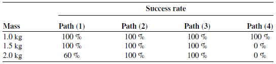
The robot traveled on the external Path (1)–(4) using only the wheel drive. When a 2.0 kg weight was mounted on the robot while it was traveling on Path 1, the motor’s power supply voltage was set to 11 V; otherwise, it was set to 9 V. The success rates for each path are listed in Table VIII, and the robot movements are shown in Figures 18–21.
Success rate of running path (1)–(4).

Experiment for traveling path (1).

Experiment for traveling path (2).

Experiment for traveling path (3).

Experiment for traveling path (4).

4.2. Inner corner Path (5)–(8) travel method
When the robot moved through internal Path (5)–(8), the wheels adhered to both the floor and wall. Therefore, the strong adhesion of the wheel prevented it from rotating. Consequently, the robot became immobile. Therefore, using the front and rear pushing mechanisms, the wheels could be lifted off one of the adhesive surfaces and the robot was freed.
The travel method for Path (7) is shown in Figure 22. The robot traversed Path (7) following the steps:
Method to run through path (7).

(1) Phase 0→Phase 1
The robot moved forward from its initial state [Figure 22(a)] until the front wheels adhered to the wall [Figure 22(b)].
(2) Phase 1→Phase 2
The front wheels could not be lifted from the floor by driving alone. Therefore, by pressing the floor with the front pushing mechanism while driving the front wheels, the wheels were lifted off the floor [Figure 22(c)].
(3) Phase 2→Phase 3
The robot moved forward until the rear wheels adhered to the wall [Figure 22(d)].
(4) Phase 3→Phase 4
The robot was lifted off the floor by pressing the floor with the rear pushing mechanism while driving the rear wheels. Therefore, the robot transitioned to the wall [Figure 22(e)].
Using the travel method, the robot transitioned from the floor to the wall. Additionally, the robot could traverse other internal Paths (5), (6), and (8) using the same method.
4.3. Inner corner path (5)--(8) running experiment
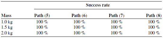
Traveling experiments were conducted on the internal Path (5)–(8). The power supply voltage of the motors was set to 9.0 V. The travel success rates for each path are listed in Table IX, and the robotic movements are shown in Figures 23, 24, 25 and 26. The robot was able to travel along Path (6) without using the method described in Section 4.2. The details are provided in a subsequent discussion.
Success rate of running path (5)–(8).

Experiment for traveling path (5).

Experiment for traveling path (6).

Experiment for traveling path (7).

Experiment for traveling path (8).

Flange section Path (9) travel method
The robot traveled along Path (9) from the underside to the top of the flange using the front pushing mechanism. The travel method on Path (9) is shown in Figure 27. The robot traversed Path (9) following the steps:
Method to traverse through path (9).

(1) Phase 0→Phase 1
The robot moved forward from its initial state [Figure 27(a)] until the front wheels moved to the top of the flange [Figure 27(b)].
(2) Phase 1→Phase 2
The front wheels rotated clockwise while the rear wheels rotated counterclockwise, causing the robot to move to the right. As a result, when the front pushing mechanism was perpendicular to the flange, the push rods pressed on the top surface of the flange [Figure 27(c)].
(3) Phase 2→Phase 3
The front pushing mechanism rotated until it was perpendicular to the flange [Figure 27(d)].
(4) Phase 3→Phase 4
While maintaining the front pushing mechanism as perpendicular to the flange as possible, the top surface of the flange was pressed with push rods. The robot was lifted until the rear chassis approached the flange [Figure 27(e)].
(5) Phase 4→Phase 5
Under the aforementioned conditions, the robot could not travel on the flange. However, when the robot was lifted further, the rear chassis came into contact with the flange. Therefore, the front wheels rotated counter-clockwise, and the rear wheels rotated clockwise. Consequently, the robot moved to a position where it was not in contact with the flange [Figure 27(f)].
(6) Phase 5→Phase 6
The robot was lifted until it traveled along Path (9) using the front pushing mechanism [Figure 27(g)]. Herein, the servomotor was subjected to a high load, making the maintenance of the front pushing mechanism perpendicular difficult. Therefore, the rotation of the mechanism did not occur.
(7) Phase 6→Phase 7
The robot moved forward to the top of the flange and completed its operation [Figure 27(h)].
4.5. Flange section Path (9) running experiment
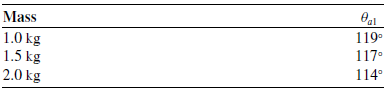
Traveling experiments were conducted from the underside to the top of the flange. The power supply voltage of the motors was set to 9.0 V. The flange thickness was 9.5 mm. When a weight was mounted, the calculated angle
 $\theta _{a1}$
that allowed the robot to travel on Path (9) is presented in Table X.
Minimum
 $\theta _{a1}$
that allows running.

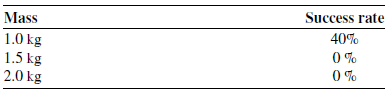
During the traveling experiments, the robot moved forward after being lifted to the maximum possible running condition. The travel success rates for each path are listed in Table XI, and the robotic movements are shown in Figure 28.
Success rate of running path (9).

Experiment of traveling path (10).

5. Considerations From the Driving Experiment
Considerations were made for Path (6), which was traversable using a method different from that described in Section 4.2, and Paths (1), (4), and (9), which the robot failed to traverse.
Path (6) involved traversing from ceiling to wall in the internal corner. During the traveling experiments on Path (6), the front wheels adhered to the wall, while the rear wheels adhered to both the ceiling and wall, as shown in Figure 29(a). In the original method, the rear wheels were lifted using a rear pushing mechanism. However, when the 2.0 kg weight was mounted, the rear wheels were lifted off using only the drive of the front wheel without the rear pushing mechanism. As shown in Figure 29(b), the robot transitioned to the wall. Therefore, gravity acting on the weight and robot was considered beneficial for lifting the rear wheels off the ceiling. Additionally, the robot could travel on internal paths without a pushing mechanism, depending on the path and weight. However, the hinge parts were subjected to high loads and could possibly break. Thus, traversing internal paths using the method should be avoided.
Successful run on path (6) using a different method.

Path (1) mapped from the wall to the floor in an external corner. During the traveling experiments on Path (1), the front and rear wheels adhered to the floor and wall, respectively, as shown in Figure 30(a). Even when the robot moved forward, the rear wheels could not transition to the floor surface, resulting in movement failure. When the front wheels reached the floor, a higher driving power was required to elevate the rear chassis and weight. Therefore, miter gears that transmitted motor torque to the wheels were subjected to high loads, and instances where the gears did not mesh properly were observed. Consequently, the motor torque was not fully transmitted to the wheels by the miter gears, causing the robot to fail to move. In addition, the front wheels did not move from the wall to the floor, as shown in Figure 30(b), because the uneven parts of the wheels could not properly catch the corners, causing the front wheels to continue slipping on the edges. Thus, considering the design of the drive-force transmission part and the shape of the wheels to easily catch the corners was crucial.
Failure to run path (1).

Path (4) mapped from the wall to the ceiling at the external corner. During the traveling experiments on Path (4), the front wheels adhered to the ceiling, and the rear wheels adhered to the wall, as shown in Figure 31(a). The robot maintained its posture while remaining stationary. However, when the robot moved forward, the rear wheels slipped, causing it to fall, as shown in Figure 31(b). The wheel slips were caused by the driving force of the rear wheels and gravity acting on the robot, which exceeded the static frictional force. Therefore, for the robot to travel along Path (4), increasing the coefficient of friction between the wheels and the riding surface was crucial.
Path (9) mapped the path from the bottom to the top of the flange. While traveling along Path (9), when the front and rear wheels were on the floor and ceiling, respectively, the chassis was lifted using the front pushing mechanism [Figure 32(a)]. Then, the robot moved forward, and the rear wheels transitioned to the floor. However, when the robot moved forward, the rear wheels occasionally slipped to the right on the underside, causing failure while traversing Path (9) [Figure 32(b)] because
 $\theta _{a1}$
was about 120°. The angle did not meet the travel conditions for 1.0, 1.5, and 2.0 kg, as listed in Table X. The more the front pushing mechanism was aslant, the less the robot was lifted compared to the amount the push rod extended. Therefore, keeping the pushing mechanism vertical to sufficiently lift the chassis was crucial. However, when the pushing mechanism was kept vertical, as the chassis was lifted, the contact points between the front wheels and riding surface, and that between the pushing mechanism and riding surface, grew closer. Consequently, the front wheels were lifted off the riding surface. Therefore, maintaining a vertical pushing mechanism was difficult. Consequently, increasing the coefficient of friction between the wheels and the riding surface was necessary to enable traversing Path (9) with a weight attached.
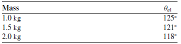
For example, the calculation in Section 3.6 was performed again with only the static friction coefficient between the wheels and the riding surface changed to 0.9. The calculated angle
 $\theta _{a1}$
that allowed the robot to travel on Path (9) is presented in Table XII. The value of
 $\theta _{a1}$
was larger than that presented in Table X. Conversely, the robot traveled with minimal lifting. Consequently, increasing the static friction coefficient was effective for traveling along Path (9).
Minimum
 $\theta _{a1}$
that allows running under the condition of static friction coefficient being 0.9.

Failure to run path (4).

Failure to run path (9) due to insufficient lifting of the robot.

In the experiment with the 2.0 kg weight, the front wheels detached from the top surface of the flange [Figure 33(a)], during the movement of the robot after the first push (Phases 4 and 5) or during the second push (Phases 5 and 6). Consequently, the robot fell [Figure 33(b)] due to the force exerted by the weight and the rod pressure on the flange, which detached the wheels. Therefore, increasing the magnetic attraction force was necessary for the robot to run with a 2.0 kg mounted weight.
Failure to run path (9) due to coming off from the flange.

Additionally, when the robot moved to the left [Figure 34(a)] (Phases 4 and 5), the robot slanted relative to the direction of movement, as shown in Figure 34(b). Therefore, when the chassis was lifted using the front pushing mechanism, the robot contacted the flange and could not move, as shown in Figure 34(c). The mechanism was attributed to the differences in the characteristics of each motor, although the same type of motor was used, and to the uneven distribution of the weight load on the left and right wheels. Therefore, the same failure could occur even without mounting a 2.0 kg weight. Consequently, to ensure that the robot traveled along Path (9), recognizing the posture of the robot and properly controlling the wheel rotation were necessary.
Failure to run path (9) due to contact with the flange.

6. Conclusions
This study proposes a method for traveling over a flange using a pushing mechanism. In addition, static analysis and running experiments are performed with the constructed magnetic-wheeled robot. The following conclusions are drawn from this study.
-
1. A static analysis of robot posture was conducted when the robot traveled from the underside to the top of the flange. Consequently, results suggested that the more the chassis was lifted, the more easily the robot traveled from the underside to the top of the flange. Additionally, by lifting the chassis to an angle greater than a certain threshold using the pushing mechanism, the adverse effects on travel caused by gravity and counter-torque of the motors were reduced. Consequently, the robot traversed the flange. In addition, the calculation results were compared with the experimental data and confirmed that the calculation results were generally accurate.
-
2. The robot was confirmed to travel all paths while carrying a 1.0 kg weight. Notably, this study demonstrated the robot’s ability to traverse from the underside to the topside of the flange while carrying a weight, which has not been shown in previous studies [Reference Tanida, Ono, Kobayashi, Shiba and Takada27, Reference Kawamoto, Matsumura and Takada28]. These results indicate that changing the robot’s posture using the pushing mechanism is effective. However, the proposed method required approximately two minutes to complete the traversal, which is more than three times longer than the 40 s reported in a previous study [Reference Tanida, Ono, Kobayashi, Shiba and Takada27]. Future work will focus on increasing the driving speed. Additionally, the impact on travel varied, depending on the mounting location of the inspection device. Therefore, further experiments using mounted devices are necessary.
-
3. The wheels and traveling surface were both made of metal. Therefore, the coefficient of friction was low, and the wheels tended to slip during travel. Consequently, the robot sometimes failed to travel along the external and flange paths. To achieve stable travel, increasing the adhesion force and the coefficient of friction between the wheels and the traveling surface is necessary. Therefore, the thickness of the iron yoke of the wheels can be increased to enhance the adhesion force, and the wheels can be coated with rubber to increase friction.
As a future prospect, dynamic analysis and control system design are important to ensure that the robot can reliably traverse through three-dimensional paths. Modeling the robot and contact forces are essential for dynamic analysis. Various models of contact force are summarized in reference [Reference Skrinjar, Slavič and Boltežar34], which is useful. Additionally, literature [Reference Enferadi and Jafari35, Reference Lin, Wang, Xu and Gao36] that conducts dynamic analysis of robot using Kane’s method can be referred to. Since this robot experiences contact with the ground surface, a robust control system design is considered necessary. Therefore, the literature [Reference Shafei, Bahrami and Talebi37, Reference Wang, Chen and Zhang38], which discusses the control system design for systems with uncertainties, provides valuable insights.
Acknowledgment
This paper was edited for English language by Editage (www.editage.jp).
Author contributions
All members conceived and designed the study. K. Ono conducted data gathering and wrote the manuscript.
Financial support
This study was supported by JST SPRING (grant number JPMJSP2139) and Measurement industry Co., Ltd.
Conflicts of interest
This study received financial support from Measurement industry Co., Ltd., which may have an interest in the results of the research. In addition, a related patent application is currently pending. No other conflicts of interest are declared.
Ethical approval
Not applicable.