1 Introduction
Transport in magnetic confinement devices is dominated by turbulent fluctuations which originate from small scale instabilities that evolve nonlinearly. The low frequency fluctuations are usually due to drift waves that extract energy from pressure gradients. The study of turbulence and the associated transport involves multiple scales, which can only be tackled by numerical simulations since analytical treatments are extremely hard. Gyrokinetic models have become a widely used tool for numerical simulations of turbulent transport (for a review see Garbet et al. Reference Garbet, Idomura, Villard and Watanbe2010), but unfortunately they are quite expensive and the interpretation of the results is not straightforward. For this reason, it is convenient to perform studies with simpler models that incorporate the essential physical effects. One such scenario is to consider transport in the limit of weak turbulence where the fluctuation spectrum can be assumed fixed and particles move in this field. These models are not self-consistent since they neglect the back reaction of particle motion on turbulence, but can provide a reasonable description of transport when fluctuation levels are not too high.
Test particles can be used advantageously to study transport in a simpler way than considering the self-consistent treatment involving turbulence theories. For electrostatic turbulence the main transport is due to
 $\boldsymbol{E}\times \boldsymbol{B}$
velocities in the fluctuating electric fields (
 $\boldsymbol{E}$
) in presence of the magnetic field (
 $\boldsymbol{B}$
). fields. The behaviour of a single particle is then described by equations of motion for the guiding centre that, for a constant magnetic field, can be cast in the form of a Hamiltonian system, which can be studied using the well-known standard techniques developed for such systems. In particular, the transition to chaos that occurs for time-dependent non-integrable Hamiltonians leads to the establishment of chaotic transport and the conditions for this to happen can be determined. This procedure has been applied in many cases considering different kinds of fluctuating fields involving various numbers of modes. The simplest situation that already exhibits chaotic behaviour is particle dynamics in the presence of two waves with different phase velocities (Kleva & Drake Reference Kleva and Drake1984; del Castillo-Negrete Reference del Castillo-Negrete2000). The relative phase velocity of the waves and its relation to the associated
 $\boldsymbol{E}\times \boldsymbol{B}$
drift velocity determines the conditions for transition to global chaos. In the weak turbulence regime, characterized by a continuum (infinite) spectrum of non-interacting waves, transport becomes more complex (Horton Reference Horton2017). However, if all the waves are assumed to have the same amplitude and wave number, the
 $\boldsymbol{E}\times \boldsymbol{B}$
equations of motion can be reduced to a Hamiltonian symplectic (area preserving) discrete map (see for example Kleva & Drake Reference Kleva and Drake1984; Horton et al.
Reference Horton, Park, Kwon, Strozzi, Morrison and Choi1998). In this case, quasilinear arguments imply that, in the limit of widespread stochasticity, transport is diffusive with a diffusivity proportional to the square of the wave amplitude. When there is a background flow in addition to the waves, particles experience also advection along the flow and the transport properties depend on the shear of the background flow. The case of monotonic shear flows with two drifts waves was studied by del Castillo-Negrete (Reference del Castillo-Negrete1998, Reference del Castillo-Negrete2000). On the other hand, as discussed by del Castillo-Negrete & Morrison (Reference del Castillo-Negrete and Morrison1993) and del Castillo-Negrete (Reference del Castillo-Negrete2000), non-monotonic shear flows are particularly interesting due to the ubiquitousness of the transport barrier associated with robust invariant shearless KAM (Kolmogorov–Arnold–Moser) curves characteristic of non-twist Hamiltonian systems.
It is convenient to emphasize that test-particle models are not self-consistent, which limits the applicability of the results. In this respect, studies using these models do not include modifications of the turbulent fluctuations due to the particle transport and thus cannot describe equilibrium patterns. Applicability is limited to short time behaviour and to small particle response. For the cases with a background flow mentioned above, the possible modification of the transport barrier produced by the particle dynamics is not accounted for, although this is a question of significant interest in problems of transport barrier dynamics (e.g. Chôné et al. Reference Chôné, Beyer, Sarazin, Fuhr, Bourdelle and Benkadda2015). Additionally, if the particle dynamics has a strong response to the wave spectrum, as will be found in this work when a flow is included (where super-ballistic transport results), it is likely that the spectrum will be modified, but this effect should be studied separately.
An important physical aspect that is not included in the
 $\boldsymbol{E}\times \boldsymbol{B}$
guiding centre descriptions discussed above is the role of finite Larmor radius (FLR) effects. Gustafson, del Castillo-Negrete & Dorland (Reference Gustafson, del Castillo-Negrete and Dorland2008) studied these effects by gyroaveraging the
 $\boldsymbol{E}\times \boldsymbol{B}$
test-particle Hamiltonian in the case of two drift waves in a monotonic shear flow. It was found that transport can be non-diffusive in the direction of the flow and that FLR effects can give rise to non-Gaussian probability distribution functions (PDF) with long tails. FLR effects have also been studied in non-monotonic zonal flows by Martinell & del Castillo-Negrete (Reference Martinell and del Castillo-Negrete2013) where it was observed that they have a stabilizing effect in the sense that the level of Hamiltonian chaos is reduced as the Larmor radius increases. This means that particles with a larger Larmor radius have less transport. A similar result was found by Dewhurst, Hnat & Dendy (Reference Dewhurst, Hnat and Dendy2010) where FLR effects in drift-wave turbulence were shown to reduce the radial transport rate in cases without (Manfredi & Dendy Reference Manfredi and Dendy1997) and with zonal flows. However, the transport along the flow direction has a superdiffusive scaling and increases with the Larmor radius. More recently, FLR effects have been studied in the context of Hamiltonian map models of transport in monotonic and non-monotonic flows with a continuum spectrum of drift waves with a one-dimensional spatial structure (da Fonseca, del Castillo-Negrete & Caldas Reference da Fonseca, del Castillo-Negrete and Caldas2014; da Fonseca et al.
Reference da Fonseca, del Castillo-Negrete, Sokolov and Caldas2016).
The more general case of an infinite spectrum of waves with a two-dimensional spatial structure propagating along the
 $y$
-direction (poloidal direction in a tokamak geometry) is of interest because the oscillations in the two spatial directions couple the
 $x$
(radial direction in a tokamak geometry) and the
 $y$
degrees of freedom of the particle. In this case, if all the waves are assumed to have the same wavenumber (
 $k_{i}=k$
) and there is no background shear flow, the
 $\boldsymbol{E}\times \boldsymbol{B}$
guiding centre dynamics (i.e. ignoring FLR effects) is described by the area preserving Hamiltonian map (Kleva & Drake Reference Kleva and Drake1984)
 $$\begin{eqnarray}\displaystyle & x_{+}^{n+1}=x_{+}^{n}-A\sin kx_{-}^{n} & \displaystyle\end{eqnarray}$$
 $$\begin{eqnarray}\displaystyle & x_{-}^{n+1}=x_{-}^{n}+A\sin kx_{+}^{n+1}, & \displaystyle\end{eqnarray}$$
where
 $x_{\pm }=x\pm y$
. Here,
 $A$
is the wave amplitude and
 $n$
refers to the iteration number. The properties of this mapping were studied by Karney (Reference Karney1979) in a study of heating by lower-hybrid waves. In the case of a spectrum of one-dimensional waves propagating along
 $y$
with a linear monotonic shear flow (i.e.
 $v_{y}\sim x$
, where
 $v_{y}$
is the flow velocity in
 $y$
direction) transport is described by the well-known standard map which was studied by Horton et al. (Reference Horton, Park, Kwon, Strozzi, Morrison and Choi1998). This case was extended by da Fonseca et al. (Reference da Fonseca, del Castillo-Negrete and Caldas2014) to include FLR effects where the gyroaveraged standard map (GSM) was introduced to study the resulting transport.
In the present paper we extend the model in (1.1)–(1.2) to include FLR effects. Our specific goal is to study the role of FLR effects on transport in the weak turbulence regime characterized by an infinite spectrum of waves oscillating in the
 $x$
and
 $y$
directions. We first address the case with no background flow and show that the FLR effects tend to maintain non-chaotic orbits until larger wave amplitudes are reached. When the amplitude is large enough to have global chaos for a given Larmor radius, the transport is diffusive. Considering the more realistic case of a thermal plasma with a Maxwellian distribution of Larmor radii, the particle distribution functions (PDF) become non-Gaussian but the transport scaling with time still shows a diffusive character. This feature can be understood with a weighted superposition of Gaussian PDFs. Then, a sheared background flow is introduced which is found to have a strong effect on the transport parallel to the flow. In particular, it produces super-ballistic transport due to a coupling of parallel and perpendicular transport. The perpendicular transport remains diffusive although the diffusion coefficient is enhanced by the flow.
The rest of the paper is organized as follows. In § 2 we describe the transport model used in the analysis of test-particle motion, starting from the guiding centre description and generalizing it to include FLR effects by the appropriate gyroaveraging. The phase space properties of the relevant mapping are described focusing on the Larmor radius dependence. The nature of transport is described in § 3 first for a fixed FLR and later for a thermal distribution of Larmor radii. Section 4 includes the presence of a background flow obtaining a modified mapping and showing that it produces super-ballistic transport. Finally, the conclusions are given in § 5.
2 Transport models
We study transport following a Lagrangian treatment in which a large ensemble of particles is considered whose motions are determined by a prescribed electrostatic field representing drift waves (and possibly an ordered flow). A test-particle approach is followed, so that particles do not modify the fields. This means self-consistency requirements are not enforced but it allows us to perform analytical studies which usually provide simple interpretations.
2.1 Guiding centre model
To first order, the motion of a charged particle in a magnetic field can be described by the motion of its guiding centre. For a constant magnetic field
 $\boldsymbol{B}=B_{0}\hat{\boldsymbol{z}}$
the guiding centre moves at the
 $\boldsymbol{E}\times \boldsymbol{B}$
drift velocity and therefore the trajectory is described by the following equation
 $$\begin{eqnarray}\frac{\text{d}\boldsymbol{r}}{\text{d}t}=\frac{\boldsymbol{E}\times \boldsymbol{B}}{B^{2}},\end{eqnarray}$$
where
 $\boldsymbol{E}$
is the electrostatic field, and
 $\boldsymbol{B}$
is the magnetic field and
 $\boldsymbol{r}$
is the particle position. The particle position can be assumed to be the same as the guiding centre position
 $\boldsymbol{r}=(x,y)$
, when the Larmor radius is small. If the electric field is expressed in terms of the electrostatic potential
 $\boldsymbol{E}=-\unicode[STIX]{x1D735}\unicode[STIX]{x1D719}^{\prime }(x,y,t)$
, the particle dynamics obtained from (2.1) can be written as a Hamiltonian system
 $$\begin{eqnarray}\frac{\text{d}x}{\text{d}t}=-\frac{\unicode[STIX]{x2202}\unicode[STIX]{x1D719}}{\unicode[STIX]{x2202}y},\quad \frac{\text{d}y}{\text{d}t}=\frac{\unicode[STIX]{x2202}\unicode[STIX]{x1D719}}{\unicode[STIX]{x2202}x},\end{eqnarray}$$
where
 $\unicode[STIX]{x1D719}$
plays the role of the Hamiltonian, while the spatial coordinates
 $(x,y)$
are the canonical conjugate phase space variables. Here the potential has been normalized to
 $\unicode[STIX]{x1D719}=\unicode[STIX]{x1D719}^{\prime }/B$
to eliminate the magnetic field.
In the test-particle weak turbulence approximation adopted here, the spectrum of waves drives the particle dynamics but the wave–wave interactions are neglected as well as the feedback of the particles to the waves. To study particle dynamics in this approximation we choose a broad drift-wave spectrum consisting of an infinite number of waves propagating in the
 $y$
-direction which is associated with the poloidal direction in a toroidal plasma. Additionally, there is an oscillatory variation along the
 $x$
direction which represents the radial direction. To simplify the analysis all waves are assumed to have the same wavenumber
 $k$
and amplitude but different velocities, which are positive and negative multiples of a fundamental frequency,
 $\unicode[STIX]{x1D714}_{0}$
. That is, we adopt the following model for the electrostatic potential
 $$\begin{eqnarray}\unicode[STIX]{x1D719}(x,y,t)=A\mathop{\sum }_{n=-\infty }^{\infty }\cos (x+\unicode[STIX]{x1D703}_{n})\cos (y+\unicode[STIX]{x1D703}_{n}-nt),\end{eqnarray}$$
where, following Kleva & Drake (Reference Kleva and Drake1984), the phases
 $\unicode[STIX]{x1D703}_{n}$
are
 $\unicode[STIX]{x1D703}_{n}=0$
if
 $n$
is even and
 $\unicode[STIX]{x1D703}_{n}=\unicode[STIX]{x03C0}/2$
if
 $n$
is odd. This introduces a
 $\unicode[STIX]{x03C0}/2$
phase difference between successive waves in the spectrum. By symmetry, choosing
 $\unicode[STIX]{x1D703}_{n}=0$
for all
 $n$
amounts to simply double the wave’s amplitude. The variables we use are normalized according to
 $x,y\rightarrow kx,ky$
,
 $t\rightarrow \unicode[STIX]{x1D714}_{0}t$
,
 $A\rightarrow (k^{2}/\unicode[STIX]{x1D714}_{0})(\unicode[STIX]{x1D719}_{1}/B)$
where
 $\unicode[STIX]{x1D719}_{1}$
is the electric potential wave amplitude. Notice that
 $A$
represents the ratio of the electric drift velocity associated with the fluctuations to the fundamental fluctuation phase speed,
 $v_{\unicode[STIX]{x1D719}}=\unicode[STIX]{x1D714}_{0}/k$
. Alternatively, it can also be written in terms of the electrostatic energy of the fluctuations,
 $W_{E}$
, relative to the magnetic energy of the magnetic guide field,
 $W_{B}$
, as
 $A=(W_{E}/W_{B})^{1/2}(c/v_{\unicode[STIX]{x1D719}})$
.
Using the identities
 $$\begin{eqnarray}\displaystyle & \displaystyle \mathop{\sum }_{n=-\infty }^{\infty }\cos (nt)=2\unicode[STIX]{x03C0}\mathop{\sum }_{m=-\infty }^{\infty }\unicode[STIX]{x1D6FF}(t-2\unicode[STIX]{x03C0}m), & \displaystyle\end{eqnarray}$$
 $$\begin{eqnarray}\displaystyle & \displaystyle \mathop{\sum }_{n=-\infty }^{\infty }(-1)^{n}\cos (nt)=2\unicode[STIX]{x03C0}\mathop{\sum }_{m=-\infty }^{\infty }\unicode[STIX]{x1D6FF}(t-(2m+1)\unicode[STIX]{x03C0}) & \displaystyle\end{eqnarray}$$
the potential in (2.3) can be written as a sum of jumps every period of the fundamental frequency
 $$\begin{eqnarray}\unicode[STIX]{x1D719}=\unicode[STIX]{x03C0}A\mathop{\sum }_{m=-\infty }^{\infty }\left[\cos (x+y)\unicode[STIX]{x1D6FF}(t-(2m+1)\unicode[STIX]{x03C0})+\cos (x-y)\unicode[STIX]{x1D6FF}(t-2\unicode[STIX]{x03C0}m)\right].\end{eqnarray}$$
Substituting (2.6) into (2.2) the equations of motion can be written in terms of the variables
 $x_{\pm }=x\pm y$
as
 $$\begin{eqnarray}\displaystyle \frac{\text{d}x_{+}}{\text{d}t} & = & \displaystyle -2\unicode[STIX]{x03C0}A\mathop{\sum }_{m=-\infty }^{\infty }\sin (x_{-})\unicode[STIX]{x1D6FF}(t-2\unicode[STIX]{x03C0}m).\end{eqnarray}$$
 $$\begin{eqnarray}\displaystyle \frac{\text{d}x_{-}}{\text{d}t} & = & \displaystyle 2\unicode[STIX]{x03C0}A\mathop{\sum }_{m=-\infty }^{\infty }\sin (x_{+})\unicode[STIX]{x1D6FF}(t-(2m+1)\unicode[STIX]{x03C0}).\end{eqnarray}$$
The periodic delta functions allow us to reduce the equations to a map in two steps, one for each of the equations in (2.7) and (2.8). When combined to a single step the resulting map is (Kleva & Drake Reference Kleva and Drake1984)
 $$\begin{eqnarray}\displaystyle x_{+}^{n+1} & = & \displaystyle x_{+}^{n}-2\unicode[STIX]{x03C0}A\sin (x_{-}^{n})\end{eqnarray}$$
 $$\begin{eqnarray}\displaystyle x_{-}^{n+1} & = & \displaystyle x_{-}^{n}+2\unicode[STIX]{x03C0}A\sin (x_{+}^{n+1}).\end{eqnarray}$$
2.2 Gyroaveraged model
The zero Larmor radius approximation described above is not valid when the particle energies are high or when the electric fields vary on a relatively small spatial scale, since then the fields experienced by the particle in its orbit are quite different from those at the guiding centre position. For these cases it is necessary to include FLR effects which can be done in a simple way by averaging the motion of the particle over one gyro-orbit. In this way, the
 $\boldsymbol{E}\times \boldsymbol{B}$
velocity on the right-hand side of (2.2), is replaced by its value averaged over a ring of radius
 $\unicode[STIX]{x1D70C}$
, where
 $\unicode[STIX]{x1D70C}$
is the Larmor radius (Lee Reference Lee1987). Then, defining the gyrophase average of a function
 $\left\langle \unicode[STIX]{x1D709}\right\rangle _{\unicode[STIX]{x1D703}}$
as
 $$\begin{eqnarray}\langle \unicode[STIX]{x1D709}\rangle _{\unicode[STIX]{x1D703}}\equiv \frac{1}{2\unicode[STIX]{x03C0}}\int _{0}^{2\unicode[STIX]{x03C0}}\unicode[STIX]{x1D709}\left(x+\unicode[STIX]{x1D70C}\cos \unicode[STIX]{x1D703},y+\unicode[STIX]{x1D70C}\sin \unicode[STIX]{x1D703}\right)\text{d}\unicode[STIX]{x1D703}\end{eqnarray}$$
the gyroaveraged equations take the form
 $$\begin{eqnarray}\frac{\text{d}x}{\text{d}t}=-\left\langle \frac{\unicode[STIX]{x2202}\unicode[STIX]{x1D719}}{\unicode[STIX]{x2202}y}\right\rangle _{\unicode[STIX]{x1D703}}=-\frac{\unicode[STIX]{x2202}\left\langle \unicode[STIX]{x1D719}\right\rangle _{\unicode[STIX]{x1D703}}}{\unicode[STIX]{x2202}y},\quad \frac{\text{d}y}{\text{d}t}=\left\langle \frac{\unicode[STIX]{x2202}\unicode[STIX]{x1D719}}{\unicode[STIX]{x2202}x}\right\rangle _{\unicode[STIX]{x1D703}}=-\frac{\unicode[STIX]{x2202}\left\langle \unicode[STIX]{x1D719}\right\rangle _{\unicode[STIX]{x1D703}}}{\unicode[STIX]{x2202}x}.\end{eqnarray}$$
This procedure is similar to the one followed in gyrokinetic models where one follows the motion of the guiding centre but FLR effects are retained. This is appropriate for studying frequencies smaller than the gyrofrequency.
Regular particle orbits in phase space due to infinite spectrum of waves with FLR effects included. There is a periodic array of closed orbits with elliptic and hyperbolic points. Here the wave amplitude is
 $A=0.1$
and the Larmor radius is (a)
 $\unicode[STIX]{x1D70C}=0$
, (b)
 $\unicode[STIX]{x1D70C}=0.7$
.

Applying this averaging to (2.3) gives
 $$\begin{eqnarray}\langle \unicode[STIX]{x1D719}\rangle _{\unicode[STIX]{x1D703}}=\frac{A}{2\unicode[STIX]{x03C0}}\int _{0}^{2\unicode[STIX]{x03C0}}\left[\mathop{\sum }_{n=-\infty }^{\infty }\cos (x+\unicode[STIX]{x1D70C}\cos \unicode[STIX]{x1D703}+\unicode[STIX]{x1D703}_{n})\cos (y+\unicode[STIX]{x1D70C}\sin \unicode[STIX]{x1D703}+\unicode[STIX]{x1D703}_{n}-nt)\right]\text{d}\unicode[STIX]{x1D703}.\end{eqnarray}$$
The same procedure described in the previous subsection can be applied to this gyroaveraged Hamiltonian to convert the resulting differential equation into a one-step map. The averages over the gyrophase are reduced using the integral representation of the Bessel function of order 0 as
 $J_{0}(x)=1/2\unicode[STIX]{x03C0}\int _{0}^{2\unicode[STIX]{x03C0}}\cos (x\sin \unicode[STIX]{x1D703})\,\text{d}\unicode[STIX]{x1D703}$
. The result is
 $$\begin{eqnarray}\displaystyle x_{+}^{n+1} & = & \displaystyle x_{+}^{n}-2\unicode[STIX]{x03C0}AJ_{0}(\sqrt{2}\unicode[STIX]{x1D70C})\sin (x_{-}^{n})\end{eqnarray}$$
 $$\begin{eqnarray}\displaystyle x_{-}^{n+1} & = & \displaystyle x_{-}^{n}+2\unicode[STIX]{x03C0}AJ_{0}(\sqrt{2}\unicode[STIX]{x1D70C})\sin (x_{+}^{n+1}),\end{eqnarray}$$
where
 $\unicode[STIX]{x1D70C}$
is the Larmor radius. Alternatively, one can arrive at this model by first gyroaveraging the equations of motion in (2.7) and then constructing the map, or by directly gyroaveraging of the guiding centre map in (2.9).
2.3 Dependence of phase space topology on FLR effects
The map resulting from the gyroaverage can be represented in the
 $xy$
plane to determine the corresponding topology of the particle trajectories. This is shown in figure 1(a) for zero Larmor radius i.e. with no FLR effects. The amplitude of the waves is quite small (
 $A=0.1$
) to make sure the motion is mostly regular. It is clear that the particles are trapped in the waves, describing closed orbits. The fixed points, defined by
 $x_{+}^{n+1}=x_{+}^{n}\equiv x_{+}^{\ast }$
and
 $x_{-}^{n+1}=x_{-}^{n}\equiv x_{-}^{\ast }$
are given by
 $\sin (x_{\pm }^{\ast })=0$
. This implies that, in terms of
 $x$
and
 $y$
,
 $x^{\ast }=(k+l)\unicode[STIX]{x03C0}/2$
and
 $y^{\ast }=(k-l)\unicode[STIX]{x03C0}/2$
with
 $k$
and
 $l$
integers. The stability analysis shows that these fixed points are stable (elliptic) when
 $k+l$
is even, whereas for odd
 $k+l$
they are hyperbolic points. This character of the fixed points can be observed in figure 1(a); for instance
 $(x,y)=(0,0),(0,\unicode[STIX]{x03C0}),(0,2\unicode[STIX]{x03C0})$
, corresponding to
 $(k,l)=(0,0),(1,-1),(2,-2)$
are elliptic points and
 $(x,y)=(\unicode[STIX]{x03C0}/2,\unicode[STIX]{x03C0}/2),(\unicode[STIX]{x03C0}/2,3\unicode[STIX]{x03C0}/2)$
, corresponding to
 $(k,l)=(1,0),(2,-1)$
are hyperbolic points.
As the wave amplitude increases the presence of chaos becomes apparent near the hyperbolic points and the remaining closed orbits around elliptic points are squeezed. Eventually, when the amplitude is large enough, there will be global chaos. Figure 2(a) shows the small regions of regular motion within the large chaotic region, for
 $A=0.4$
.
The effect of FLR is to stabilize the destabilizing nonlinear effect of the large amplitudes as seen in figures 1(b) and 2(b) which show the phase space for
 $\unicode[STIX]{x1D70C}=0.7$
for the same amplitudes as figures 1(a) and 2(a). When chaos is not apparent there is no appreciable difference with FLR. However, when there is already chaos, as for the amplitude
 $A=0.4$
, the phase space is less chaotic when the Larmor radius is increased up to a value
 $\unicode[STIX]{x1D70C}=x_{01}$
, where
 $x_{01}$
is the first zero of the Bessel function
 $J_{0}(x)$
. If
 $\unicode[STIX]{x1D70C}$
is further increased then the chaotic region gets larger again. This behaviour is repeated according to the oscillating variation of
 $J_{0}(x)$
.
Growth of chaos in phase space for large amplitude
 $A=0.4$
showing bifurcation of elliptic points for
 $\unicode[STIX]{x1D70C}=0$
in (a) an with a finite Larmor radius
 $\unicode[STIX]{x1D70C}=0.7$
in (b) showing a reduction of the chaotic region.

3 Non-diffusive transport due to FLR effects
In this section we discuss numerical results showing evidence of non-diffusive transport due to FLR effects. In particular, it is shown that for a thermal Maxwellian distribution of Larmor radii, particle displacements do not exhibit the Gaussian dependence observed in the case of zero Larmor radius dynamics.
The gyroaveraged map in (2.14)–(2.15) exhibits fairly regular motion for low amplitude
 $A$
and it becomes increasingly chaotic as
 $A$
grows. As mentioned above, chaos appears first around hyperbolic points and it extends to larger regions. For small
 $A$
, a significant fraction of the particles is trapped and moves periodically in well-localized regions of phase space. These closed orbits around the elliptic points form invariant surfaces which are elongated as
 $A$
grows and those farther from the O-point are destroyed. As shown in figure 2(a), when the amplitude
 $A$
exceeds a critical value
 $A_{c}$
the period-one elliptic points bifurcate into two period-2 O-points. At larger amplitudes these regions are eventually lost and there is widespread stochasticity in the system. As observed by comparing (2.9)–(2.10) and (2.14)–(2.15), the main role of the Larmor radius is to rescale the amplitude of the map by the factor
 $J_{0}(\sqrt{2}\unicode[STIX]{x1D70C})$
. Accordingly, if
 $A_{c0}$
denotes the critical value of the amplitude in the absence of FLR effects, then the corresponding critical amplitude for Larmor radius
 $\unicode[STIX]{x1D70C}$
is
 $$\begin{eqnarray}A_{c}=\frac{A_{c0}}{J_{0}(\sqrt{2}\unicode[STIX]{x1D70C})}\approx A_{c0}\left(1+\frac{\unicode[STIX]{x1D70C}^{2}}{2}\right),\end{eqnarray}$$
where the last expression assumes small
 $\unicode[STIX]{x1D70C}$
. The numerical value of
 $A_{c0}$
is found to be
 $A_{c0}\approx 0.3184$
.
Trapped particle fraction (i.e. particles not reaching a surface at
 $r=10$
after 100 iterations) from a thermal distribution of Larmor radii for three values of the thermal radius:
 $\unicode[STIX]{x1D70C}_{th}=0.7$
(green), 1 (blue) and 1.5 (red). Dashed lines are for the initial population at elliptic point (0,0), continuous lines for hyperbolic point (
 $\unicode[STIX]{x03C0}/2,\unicode[STIX]{x03C0}/2$
).

As is well known, in the absence of FLR effects (i.e. for
 $\unicode[STIX]{x1D70C}=0$
), in the weak turbulence limit (i.e. for large values of
 $A$
) there is widespread stochasticity and particles exhibit diffusive Brownian motion. In particular, an ensemble of particles initially located in a small square around
 $(x,y)=(x^{0},y^{0})$
exhibits Gaussian spreading in the
 $x$
and
 $y$
directions. That is, if
 $P_{x}(\unicode[STIX]{x1D6FF}x,t)$
denotes the probability density of displacements in the
 $x$
-direction at time
 $t$
and fixed
 $y=y^{0}$
, then
 $P_{x}(\unicode[STIX]{x1D6FF}x,t)=(1/\unicode[STIX]{x1D70E}_{x}\sqrt{2\unicode[STIX]{x03C0}})\exp (-\unicode[STIX]{x1D6FF}x^{2}/2\unicode[STIX]{x1D70E}_{x})$
where
 $\unicode[STIX]{x1D70E}_{x}=\unicode[STIX]{x1D70E}_{x}(t)$
denotes the variance, with a similar expression for the displacements in
 $y$
. Note that due to isotropy, the variance of the displacements in the
 $x$
and
 $y$
directions is the same. From here it follows that the probability density of radial displacements,
 $r=\sqrt{\unicode[STIX]{x1D6FF}x^{2}+\unicode[STIX]{x1D6FF}y^{2}}$
, is the Rayleigh distribution
 $P(\unicode[STIX]{x1D6FF}r,t)=(1/\unicode[STIX]{x1D70E}^{2})r\exp (-\unicode[STIX]{x1D6FF}r^{2}/2\unicode[STIX]{x1D70E})$
. Moreover, the variance
 $\unicode[STIX]{x1D70E}(t)=\langle r^{2}\rangle =\int _{0}^{\infty }r^{2}P(\unicode[STIX]{x1D6FF}r,t)\,\text{d}r$
exhibits the well-known diffusive linear scaling with time
 $\unicode[STIX]{x1D70E}(t)\sim t$
. When the time evolution is discrete, as in the case of the discrete area preserving maps of interest in this paper,
 $\unicode[STIX]{x1D70E}(n)\sim n$
where
 $n$
is the iteration number and
 $\unicode[STIX]{x1D70E}(n)=\sum _{i}(r_{i}^{n}-r_{i}^{0})^{2}\approx \sum _{i}(r_{i}^{n})^{2}$
with
 $r_{i}^{n}$
denoting the radial displacement of the
 $i$
th particle at time
 $n$
, assuming the initial position
 $r_{i}^{0}\ll r_{i}^{n}$
. In the highly chaotic regime there is no difference in the location of the initial condition; only when chaos is starting to spread out is there a distinction in the transport depending on whether
 $(x^{0},y^{0})$
is an elliptical or a hyperbolic point. This is exemplified in figure 3 where the fraction of particles remaining within a region bounded by a distant surface after a time
 $t$
is plotted for the two types of initial positions. For
 $A\gg 1$
all cases tend to the same value. Following da Fonseca et al. (Reference da Fonseca, del Castillo-Negrete, Sokolov and Caldas2016), in this figure we plot the fraction of trapped particles (i.e. not reaching the surface) as function of the amplitude
 $A$
. Two sets of curves are represented, one in which the initial population is around an elliptic point (dashed lines) and another for a hyperbolic point. For an elliptic point all particles are trapped for small
 $A$
and they start escaping after a threshold
 $A\approx 0.4$
. In the hyperbolic point case, there are always untrapped particles for any value of
 $A$
. The difference gets smaller as
 $A$
increases until it disappears for large enough
 $A$
, when global chaos practically erases any trace of elliptic or hyperbolic points.
PDF of displacements in
 $y$
of an ensemble of particles with a Maxwellian distribution of Larmor radii in (3.2) (continuous blue line) with
 $A=1$
,
 $\unicode[STIX]{x1D70C}_{th}=1$
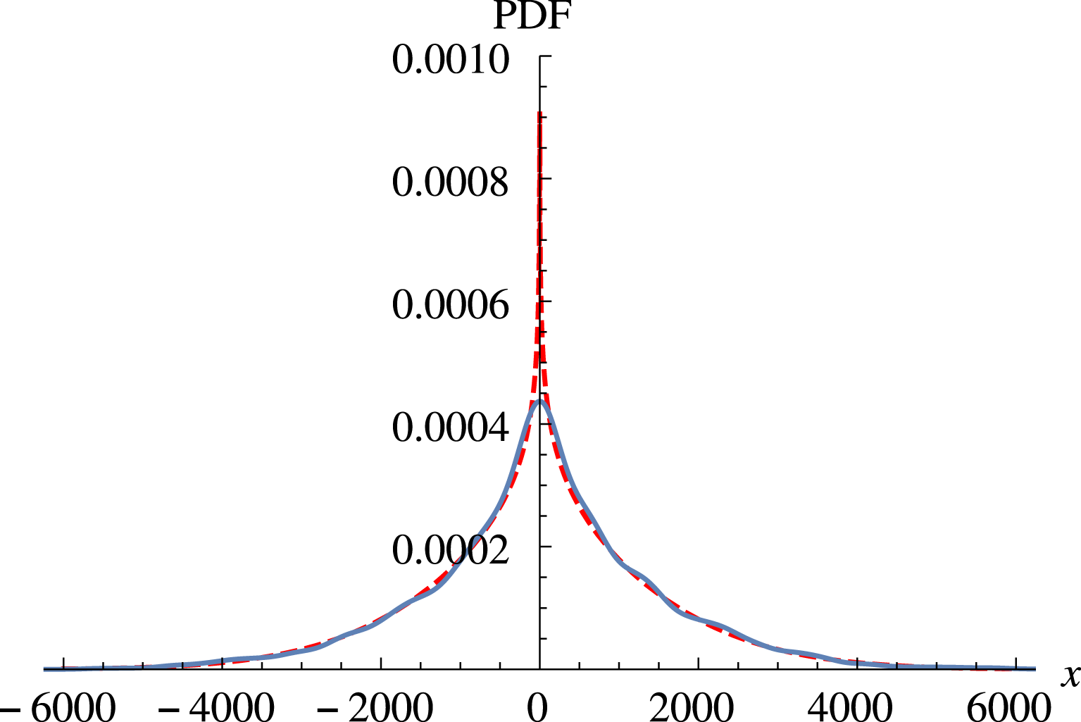
, in log–linear scale (a) and in linear scale (b). The dashed red line is the fit from (3.6). The long tails indicate an exponential-like decay as opposed to the Gaussian decay characteristic of ensembles with zero Larmor radii. Also the relatively high value of the kurtosis,
 $K=6.56$
, indicates strong departures with respect to the
 $K=3$
Gaussian case without FLR effects.

These
 $\unicode[STIX]{x1D70C}=0$
results directly apply to the FLR case provided all the particles have the same Larmor radius, i.e. provided
 $\unicode[STIX]{x1D70C}_{i}=\unicode[STIX]{x1D70C}$
for
 $i=1,2,\ldots$
where
 $\unicode[STIX]{x1D70C}_{i}$
denotes the Larmor radius of the
 $i$
th particle. This is because, as discussed before, when all the particles have the same Larmor radius, FLR effects simply rescale the wave amplitude by the factor
 $J_{0}(\sqrt{2}\unicode[STIX]{x1D70C})$
.
However, in the case when the particles have different Larmor radii, the probability distribution of displacements is in general non-Gaussian and the system can exhibit highly non-trivial statistical behaviour. The study of this problem is one of the main goals of this paper. As a starting point we assume a thermal Maxwellian equilibrium distribution function of Larmor radii of the form
 $$\begin{eqnarray}f(\unicode[STIX]{x1D70C})=(2\unicode[STIX]{x1D70C}/\unicode[STIX]{x1D70C}_{th}^{2})\exp [-(\unicode[STIX]{x1D70C}/\unicode[STIX]{x1D70C}_{th})^{2}],\end{eqnarray}$$
where
 $\unicode[STIX]{x1D70C}_{th}=\sqrt{2mk_{B}T}/(|q|B_{0})$
is the thermal Larmor radius. As before, an initial particle population with gyroradii taken from (3.2) is followed to obtain the PDF. In figure 4 the PDF for motion along the
 $y$
direction is presented in both linear and log-linear scales for the case of
 $\unicode[STIX]{x1D70C}_{th}=1$
and a wave amplitude
 $A=1$
, for which there is already global chaos. It can be seen that the distribution is non-Gaussian, which is better appreciated in the log-linear plot: the central part, near the origin, has a Gaussian shape but it transitions to a long-tailed function for large
 $|y|$
having a falloff that may be fit by a stretched exponential,
 $f(y)\sim \exp (-\unicode[STIX]{x1D6FD}y^{\unicode[STIX]{x1D6FE}})$
with
 $\unicode[STIX]{x1D6FE}\gtrsim 1$
. The kurtosis of this PDF is
 $K=6.56$
, more than twice the value of 3 for a Gaussian. In figure 5 the PDF is also shown for the same
 $\unicode[STIX]{x1D70C}_{th}$
and
 $A=20$
for which the orbits are all chaotic and the same behaviour is observed. For all the values of
 $\unicode[STIX]{x1D70C}_{th}$
and
 $A$
the PDFs have in general kurtosis of the order of 5–7, which means all cases have long tails. Incidentally, it has been checked that the PDF tends to a Gaussian as the thermal radius approaches zero (i.e.
 $T\rightarrow 0$
), as would be expected.
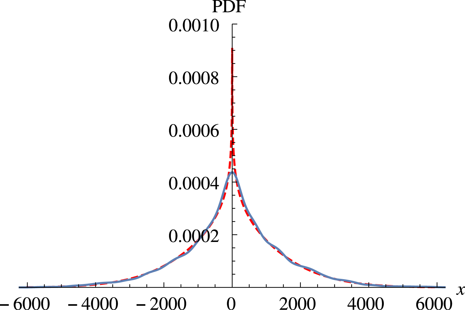
PDF from (3.6) (dashed red) for
 $\unicode[STIX]{x1D70C}_{th}=1$
and
 $A=20$
in log–linear (a) and linear (b) scales fitting the numerically obtained PDF for the same parameters (blue).

Variance of the PDF for thermal particles with
 $\unicode[STIX]{x1D70C}_{th}=1$
as function of time in log–log scale, showing the linear scaling for
 $A=1$
(lower curve) and
 $A=20$
(upper curve). The regression fit is shown with dashed lines and the corresponding equation is shown.

On the other hand, the variance increases in time as
 $\unicode[STIX]{x1D70E}_{y,th}(t)\sim t$
as can be seen in figure 6, indicating that the transport maintains a diffusive scaling. Two values of
 $A$
are shown and we see that the spread of the distribution (given by
 $\unicode[STIX]{x1D70E}_{y,th}$
) increases with
 $A$
due to the increase of chaos level. When
 $A$
is not so large there are more particles with closed orbits which do not diffuse. This effect can be appreciated better if we look at figure 3 which gives the number of particles not reaching a distant surface after a given time. It shows that the fraction of trapped particles always decreases with
 $A$
, for any value of
 $\unicode[STIX]{x1D70C}_{th}$
and it increases with
 $\unicode[STIX]{x1D70C}_{th}$
since the chaotic region is reduced.
The change of the PDF from Gaussian for a fixed Larmor radius to a heavy-tailed non-Gaussian for a thermal distribution of Larmor radii can be explained from the addition of distribution functions. It is a well-known fact that when two Gaussians with different widths are added the result is not a Gaussian but a distribution with kurtosis larger than 3. To use this fact for our case, we start by writing the PDF for a single Larmor radius,
 $\unicode[STIX]{x1D70C}=\unicode[STIX]{x1D70C}_{0}$
. Quasilinear arguments (see for example Lichtenberg & Lieberman Reference Lichtenberg and Lieberman1992) show that in the weak turbulence limit
 $$\begin{eqnarray}\displaystyle P_{\unicode[STIX]{x1D70C}_{0}}(y,t)=\frac{1}{\sqrt{2\unicode[STIX]{x03C0}D(\unicode[STIX]{x1D70C}_{0})t}}\exp \left[\frac{-y^{2}}{2D(\unicode[STIX]{x1D70C}_{0})t}\right], & & \displaystyle\end{eqnarray}$$
where the diffusion coefficient
 $D(\unicode[STIX]{x1D70C}_{0})$
can be obtained from the mapping, by constructing the cumulative square displacements, averaged over all particles (Karney Reference Karney1979)
 $$\begin{eqnarray}\displaystyle S\equiv \mathop{\sum }_{j=1}^{n}\langle (y^{j+1}-y^{j})^{2}\rangle _{p} & = & \displaystyle \frac{1}{4}\mathop{\sum }_{j=1}^{n}\langle ([x_{+}^{\,j+1}-x_{+}^{j}]-[x_{-}^{j+1}-x_{-}^{j}])^{2}\rangle _{p}\nonumber\\ \displaystyle & = & \displaystyle \frac{[A(\unicode[STIX]{x1D70C}_{0})]^{2}}{4}\mathop{\sum }_{j=1}^{n}\langle (\sin (x_{-}^{j})-\sin (x_{+}^{j+1}))^{2}\rangle _{p}\nonumber\\ \displaystyle & = & \displaystyle ([A(\unicode[STIX]{x1D70C}_{0})]^{2}/4)n,\end{eqnarray}$$
where the definition
 $A(\unicode[STIX]{x1D70C}_{0})=2\unicode[STIX]{x03C0}AJ_{0}(\sqrt{2}\unicode[STIX]{x1D70C}_{0})$
was introduced. In the last step it was assumed that the displacements have a random distribution as a result of the prevalence of chaotic orbits, which would be valid only in the large
 $A$
weak turbulence limit. The variance is
 $\unicode[STIX]{x1D70E}_{y}=\langle (y^{n}-y^{0})^{2}\rangle _{p}=S+\sum _{i=1}^{n}\sum _{j\neq i}^{n}\langle (y^{j+1}-y^{j})(y^{i+1}-y^{i})\rangle _{p}=S$
since the second term vanishes for random (independent) displacements. Then, since the iteration number plays the role of time, the diffusion coefficient is
 $$\begin{eqnarray}D(\unicode[STIX]{x1D70C}_{0})=\frac{S}{2n}=\frac{1}{2}\left[\unicode[STIX]{x03C0}AJ_{0}\left(\sqrt{2}\unicode[STIX]{x1D70C}_{0}\right)\right]^{2}.\end{eqnarray}$$
When there is a distribution of Larmor radii given by
 $f(\unicode[STIX]{x1D70C})$
, i.e. when each particle has its own
 $\unicode[STIX]{x1D70C}$
, the resulting PDF should be a weighted average over all Larmor radii, that is,
 $$\begin{eqnarray}P(y,t)=\int _{0}^{\infty }\frac{f(\unicode[STIX]{x1D70C})}{\sqrt{2\unicode[STIX]{x03C0}D_{0}J_{0}^{2}(\sqrt{2}\unicode[STIX]{x1D70C})t}}\exp \left[\frac{-y^{2}}{2D_{0}J_{0}^{2}(\sqrt{2}\unicode[STIX]{x1D70C})t}\right]\text{d}\unicode[STIX]{x1D70C},\end{eqnarray}$$
where
 $D_{0}=\unicode[STIX]{x03C0}^{2}A^{2}$
. In figures 4 and 5 we have plotted the PDF given by (3.6) with the dashed red lines to compare with the numerically obtained PDF. It is clear that there is an almost perfect fit to the non-Gaussian PDF, reproducing especially well the long tails. As expected, the agreement is better for the large
 $A$
in figure 5 although even for
 $A=1$
the matching is good.
As already seen in figure 6, the variance still exhibits diffusive scaling even though the PDF has quite heavy tails. This can be derived from the effective PDF, equation (3.6). Because of symmetry, the odd moments are zero,
 $\langle y^{2n+1}\rangle =0$
, where
 $\langle \unicode[STIX]{x1D701}\rangle =\int _{0}^{\infty }\unicode[STIX]{x1D701}P(y,t)\,\text{d}y$
. The even moments are given by
 $$\begin{eqnarray}\langle y^{2n}\rangle =\int _{0}^{\infty }\text{d}\unicode[STIX]{x1D70C}\frac{f(\unicode[STIX]{x1D70C})}{\sqrt{2\unicode[STIX]{x03C0}D_{0}J_{0}^{2}(\sqrt{2}\unicode[STIX]{x1D70C})t}}\int _{-\infty }^{\infty }y^{2n}\exp \left[\frac{-y^{2}}{2D_{0}J_{0}^{2}(\sqrt{2}\unicode[STIX]{x1D70C})t}\right]\text{d}y.\end{eqnarray}$$
From here
 $$\begin{eqnarray}\langle y^{2n}\rangle =(2n-1)!!D_{0}^{n}t^{n}\int _{0}^{\infty }\text{d}\unicode[STIX]{x1D70C}f(\unicode[STIX]{x1D70C})J_{0}^{2n}(\sqrt{2}\unicode[STIX]{x1D70C})=(2n-1)!!\langle D^{n}\rangle t^{n},\end{eqnarray}$$
which indicates that the time evolution of the moments exhibit diffusive scaling, in particular, the variance
 $\unicode[STIX]{x1D70E}=\langle y^{2}\rangle$
is
 $$\begin{eqnarray}\langle y^{2}\rangle =\langle D\rangle t,\end{eqnarray}$$
where the effective diffusion coefficient is
 $\langle D\rangle /2$
, with
 $$\begin{eqnarray}\langle D\rangle =D_{0}\text{e}^{-\unicode[STIX]{x1D70C}_{th}^{2}}I_{0}(\unicode[STIX]{x1D70C}_{th}^{2}).\end{eqnarray}$$
This is shown in figure 7 as a function of the thermal radius. We notice that for
 $\unicode[STIX]{x1D70C}_{th}\gtrsim 2$
the diffusion is considerably reduced. The expression (3.10) provides also a good representation of the slope of the line in figure 6 for the transport calculations, since, for the values in that plot,
 $10^{0.641}=4.38\approx \langle D\rangle =\unicode[STIX]{x03C0}^{2}\text{e}^{-1}I_{0}(1)=4.59$
. The quasilinear scaling
 $\langle D\rangle \sim A^{2}$
also reproduces the results of figure 6 for the two amplitudes since
 $10^{3.235}/10^{0.641}=392\approx 20^{2}$
.
Effective diffusion coefficient for the transport associated with the PDF in (3.6).

Rescaled PDF as a function of the similarity variable
 $x=y/\sqrt{\langle D\rangle t}$
for 3 different times
 $t=500$
(solid blue),
 $t=1000$
(dashed green) and
 $t=5000$
(dotted red) for the values of
 $\unicode[STIX]{x1D70C}_{th}=0.1$
(a) and
 $\unicode[STIX]{x1D70C}_{th}=1$
(b). They all collapse to a single function that depends on
 $\unicode[STIX]{x1D70C}_{th}$
. Theoretical curves are black dashed.

An interesting property is that, as shown in figure 8, the PDF in (3.6) for a thermal distribution of finite Larmor radii exhibits the self-similar scaling
 $$\begin{eqnarray}P(y,t)=\frac{1}{\sqrt{\langle D\rangle t}}{\mathcal{G}}_{\unicode[STIX]{x1D70C}_{th}}\left(\frac{y}{\sqrt{\langle D\rangle t}}\right),\end{eqnarray}$$
with a scaling function
 ${\mathcal{G}}_{\unicode[STIX]{x1D70C}_{th}}(\unicode[STIX]{x1D709})$
. The plots in figure 8 show the PDF as a function of scaled variables for two values of the thermal radius at three different times, showing that the self-similarity holds. The interesting feature is that the shape of the function
 ${\mathcal{G}}_{\unicode[STIX]{x1D70C}_{th}}(\unicode[STIX]{x1D709})$
depends on the value of the thermal radius and it is a Gaussian for small
 $\unicode[STIX]{x1D70C}_{th}$
. However, it becomes non-Gaussian for
 $\unicode[STIX]{x1D70C}_{th}$
of the order of 1. As it turns out
 ${\mathcal{G}}_{\unicode[STIX]{x1D70C}_{th}}(\unicode[STIX]{x1D709})$
has nearly exponential tails.
Dependence
 $\unicode[STIX]{x1D705}(\unicode[STIX]{x1D70C}_{th})$
of the kurtosis on the thermal radius: the theoretical dependence from (3.12) (solid blue) and the numerical dependences for
 $A=1$
(dashed orange),
 $A=5$
(dot-dashed green) and
 $A=20$
(dotted red).

The agreement of the analytical expression in (3.10) with the numerical calculations of transport is reasonable only when the mapping is sufficiently chaotic, i.e. for large
 $A$
. An analytical expression for the kurtosis can also be obtained, and is valid in the same limit. According to (3.6) it is given by
 $$\begin{eqnarray}\unicode[STIX]{x1D705}=\frac{6\text{e}^{2\unicode[STIX]{x1D70C}_{th}^{2}}}{I_{0}^{2}\left(\unicode[STIX]{x1D70C}_{th}^{2}\right)}\int _{0}^{\infty }\frac{\unicode[STIX]{x1D70C}}{\unicode[STIX]{x1D70C}_{th}^{2}}\text{e}^{-\unicode[STIX]{x1D70C}^{2}/\unicode[STIX]{x1D70C}_{th}^{2}}J_{0}^{4}\left(\sqrt{2}\unicode[STIX]{x1D70C}\right)\,\text{d}\unicode[STIX]{x1D70C}.\end{eqnarray}$$
As shown in figure 9, the agreement of this expression with the numerical results is good for large
 $A$
. This is so because, in that case, most particles in the thermal distribution, even those with large
 $\unicode[STIX]{x1D70C}$
, have chaotic orbits. For small
 $A$
the kurtosis is larger because some fraction of the particles is still trapped while the bulk population travels away from the starting point, which produces a very broad PDF. An interesting relationship can be written for the kurtosis and the diffusion coefficient
 $$\begin{eqnarray}\unicode[STIX]{x1D705}=3\frac{\langle D^{2}\rangle }{\langle D\rangle ^{2}}=3\frac{\langle J_{0}^{4}(\sqrt{2}\unicode[STIX]{x1D70C})\rangle }{[\langle J_{0}^{2}(\sqrt{2}\unicode[STIX]{x1D70C})\rangle ]^{2}}.\end{eqnarray}$$
Asymptotic expressions for large and small
 $\unicode[STIX]{x1D70C}_{th}$
can be found. As
 $\unicode[STIX]{x1D70C}_{th}$
approaches infinity
 $$\begin{eqnarray}\unicode[STIX]{x1D705}\approx \frac{6\,e^{2\unicode[STIX]{x1D70C}_{th}^{2}}}{\left[e^{\unicode[STIX]{x1D70C}_{th}^{2}}/\sqrt{2\unicode[STIX]{x03C0}\unicode[STIX]{x1D70C}_{th}^{2}}\right]^{2}}\int _{0}^{\infty }\frac{\unicode[STIX]{x1D70C}}{\unicode[STIX]{x1D70C}_{th}^{2}}J_{0}^{4}\left(\sqrt{2}\unicode[STIX]{x1D70C}\right)\text{d}\unicode[STIX]{x1D70C}\approx 12\unicode[STIX]{x03C0}\int _{0}^{\infty }\unicode[STIX]{x1D70C}J_{0}^{4}\left(\sqrt{2}\unicode[STIX]{x1D70C}\right)\text{d}\unicode[STIX]{x1D70C}\end{eqnarray}$$
evaluating the integral yields
 $$\begin{eqnarray}\unicode[STIX]{x1D705}(\unicode[STIX]{x1D70C}_{th}\rightarrow \infty )\rightarrow 12\unicode[STIX]{x03C0}(0.77085)\approx 29.06.\end{eqnarray}$$
On the other hand, when
 $\unicode[STIX]{x1D70C}_{th}\rightarrow 0$
 $$\begin{eqnarray}\unicode[STIX]{x1D705}\approx \frac{3(1+2\unicode[STIX]{x1D70C}_{th}^{2})}{\left(1+\unicode[STIX]{x1D70C}_{th}^{4}/4\right)^{2}}\int _{0}^{\infty }\left[\frac{2\unicode[STIX]{x1D70C}}{\unicode[STIX]{x1D70C}_{th}^{2}}e^{-\unicode[STIX]{x1D70C}^{2}/\unicode[STIX]{x1D70C}_{th}^{2}}\right]J_{0}^{4}\left(\sqrt{2}\unicode[STIX]{x1D70C}\right)\,\text{d}\unicode[STIX]{x1D70C}\approx 3(1+2\unicode[STIX]{x1D70C}_{th}^{2})\end{eqnarray}$$
the last step is because the term in square brackets tends to a delta function as
 $\unicode[STIX]{x1D70C}_{th}\rightarrow 0$
. This parabolic-like behaviour for small
 $\unicode[STIX]{x1D70C}_{th}$
can be noticed in figure 9. Although not shown in figure 9, the numerical computations confirm the asymptotic value
 ${\approx}29$
for
 $\unicode[STIX]{x1D70C}_{th}\gg 1$
.
It should be mentioned that, by symmetry, the same analysis made for the
 $y$
transport holds for transport along the
 $x$
direction. That is, when all the particles have the same Larmor radius the PDF of the
 $x$
-displacements is Gaussian, but when the distribution of Larmor radii is Maxwellian, the PDF is not Gaussian. However, in both cases, the variance of displacements in
 $x$
exhibits diffusive scaling in time.
4 Transport analysis in the presence of a background flow
4.1 Transport model
If, in addition to the wave spectrum, there is a background
 $\boldsymbol{E}\times \boldsymbol{B}$
flow, the potential can be modelled as
 $$\begin{eqnarray}\unicode[STIX]{x1D719}=\unicode[STIX]{x1D719}_{0}(x)+A\mathop{\sum }_{n=-\infty }^{\infty }\cos (x+\unicode[STIX]{x1D703}_{n})\cos (y+\unicode[STIX]{x1D703}_{n}-nt),\end{eqnarray}$$
where
 $\unicode[STIX]{x1D719}_{0}(x)$
represents a shear flow in the
 $y$
-direction with velocity
 $v_{0}=\text{d}\unicode[STIX]{x1D719}_{0}/\text{d}x$
. To derive the equations of motion including FLR effects, we gyroaverage the potential,
 $$\begin{eqnarray}\langle \unicode[STIX]{x1D719}\rangle =\langle \unicode[STIX]{x1D719}_{0}(x)\rangle +AJ_{0}(\sqrt{2}\unicode[STIX]{x1D70C})\mathop{\sum }_{n=-\infty }^{\infty }\cos (x+\unicode[STIX]{x1D703}_{n})\cos (y+\unicode[STIX]{x1D703}_{n}-nt),\end{eqnarray}$$
and repeat the procedure outlined in the previous section, converting a two-step map to a one-step map. This time, the new term prevents the map from being exact, but provides a discrete approximation. Thus we arrive at the symplectic discrete mapping model, which in terms of the
 $x_{\pm }$
variables can be written as
 $$\begin{eqnarray}\displaystyle x_{+}^{n+1} & = & \displaystyle x_{+}^{n}-2\unicode[STIX]{x03C0}AJ_{0}(\sqrt{2}\unicode[STIX]{x1D70C})\sin (x_{-}^{n})+\unicode[STIX]{x1D6FA}\left(\frac{x_{+}^{n}+x_{-}^{n}}{2}\right)\end{eqnarray}$$
 $$\begin{eqnarray}\displaystyle x_{-}^{n+1} & = & \displaystyle x_{-}^{n}+2\unicode[STIX]{x03C0}AJ_{0}(\sqrt{2}\unicode[STIX]{x1D70C})\sin (x_{+}^{n+1})-\unicode[STIX]{x1D6FA}\left(\frac{x_{+}^{n+1}+x_{-}^{n+1}}{2}\right),\end{eqnarray}$$
where
 $\unicode[STIX]{x1D6FA}(x^{n})=\unicode[STIX]{x03C0}[(\text{d}\langle \unicode[STIX]{x1D719}_{0}(x)\rangle /\text{d}x)^{n+1/2}+(\text{d}\langle \unicode[STIX]{x1D719}_{0}(x)\rangle /\text{d}x)^{n}]$
and
 $\unicode[STIX]{x1D6FA}(x^{n+1})=\unicode[STIX]{x03C0}[(\text{d}\langle \unicode[STIX]{x1D719}_{0}(x)\rangle /\text{d}x)^{n+1}+(\text{d}\langle \unicode[STIX]{x1D719}_{0}(x)\rangle /\text{d}x)^{n+1/2}]$
are average velocities between steps. Depending on
 $\unicode[STIX]{x1D719}_{0}(x)$
, the flow velocity
 $\unicode[STIX]{x1D6FA}(x)$
can be monotonic or non-monotonic. The first case gives rise to a twist mapping while for the second the map is non-twist.
In general, the map in (4.3)–(4.4) is implicit. For the case of a monotonic, linear velocity profile,
 $\unicode[STIX]{x1D6FA}(x)=Cx$
, it can be written in the explicit form
 $$\begin{eqnarray}\displaystyle x_{+}^{n+1} & = & \displaystyle x_{+}^{n}-2\unicode[STIX]{x03C0}AJ_{0}(\sqrt{2}\unicode[STIX]{x1D70C})\sin (x_{-}^{n})+\frac{C}{2}\left(x_{+}^{n}+x_{-}^{n}\right)\end{eqnarray}$$
 $$\begin{eqnarray}\displaystyle x_{-}^{n+1} & = & \displaystyle \frac{1}{1-C/2}\left[x_{-}^{n}+2\unicode[STIX]{x03C0}AJ_{0}(\sqrt{2}\unicode[STIX]{x1D70C})\sin (x_{+}^{n+1})-\frac{C}{2}x_{+}^{n+1}\right].\end{eqnarray}$$
Here, the dimensionless constant
 $C$
is related to the dimensional electric potential responsible of the flow
 $\unicode[STIX]{x1D719}_{0}$
by
 $C=(k^{2}/\unicode[STIX]{x1D714}_{0})(\unicode[STIX]{x1D719}_{0}/B)$
. This represents the ratio of the background flow velocity to the fluctuations’ fundamental phase speed
 $v_{\unicode[STIX]{x1D719}}$
. This mapping has to be restricted to values of
 $C<2$
since for
 $C=2$
it becomes singular.
4.2 Phase space topology
The phase space trajectories for the mapping (4.5) and (4.6) are shown in figure 10 for four different sets of parameters. The shear flow modifies the phase space topology, creating open orbits corresponding to particles streaming with the flow, when the Larmor radius is zero (see figure 10 a). In general, the presence of shear flows is related to the appearance of transport barriers. This is also the case in the present mapping that exhibits invariant tori represented by the vertical trajectories. The period-one orbits (fixed points) can be found by setting
 $$\begin{eqnarray}A(\unicode[STIX]{x1D70C})\sin x_{\pm }^{\ast }=\frac{C}{2}(x_{+}^{\ast }+x_{-}^{\ast }),\end{eqnarray}$$
with
 $A(\unicode[STIX]{x1D70C})$
defined after (3.4), which can be satisfied when
 $x_{+}^{\ast }=-x_{-}^{\ast }=k\unicode[STIX]{x03C0}$
for any integer
 $k$
. In terms of the original coordinates this means
 $(x^{\ast },y^{\ast })=(0,k\unicode[STIX]{x03C0})$
. The stability analysis shows that the fixed point is stable (elliptic) provided
 $$\begin{eqnarray}[-A(\unicode[STIX]{x1D70C})+(-1)^{k}(C-C^{2}/4)]A(\unicode[STIX]{x1D70C})+C^{3}/8<0,\end{eqnarray}$$
and unstable (hyperbolic) otherwise. When
 $\unicode[STIX]{x1D70C}$
is such that
 $J_{0}(\sqrt{2}\unicode[STIX]{x1D70C})>0$
and
 $k$
is even (as for the fixed point at the origin) the condition to be an elliptic point is
 $C^{3}/8<A(\unicode[STIX]{x1D70C})[A(\unicode[STIX]{x1D70C})-C+C^{2}/4]$
, and thus, as the wave amplitude increases, the hyperbolic points become elliptic (see figure 10
b). On the other hand, the fixed points for odd
 $k$
are elliptic and remain elliptic since the condition
 $C^{3}/8-A(\unicode[STIX]{x1D70C})[A(\unicode[STIX]{x1D70C})+C-C^{2}/4]<0$
is always fulfilled for positive
 $J_{0}(\sqrt{2}\unicode[STIX]{x1D70C})$
and small
 $C$
. For large
 $C$
, orbits are chaotic around hyperbolic points and thus there are no longer fixed points there.
Phase space trajectories for the mapping with flow when
 $C=0.5$
. (a)
 $\unicode[STIX]{x1D70C}=0$
and
 $A=0.02$
; (b)
 $\unicode[STIX]{x1D70C}=0$
and
 $A=0.1$
; (c)
 $\unicode[STIX]{x1D70C}=0.5$
and
 $A=0.1$
; (d)
 $\unicode[STIX]{x1D70C}=0.5$
and
 $A=0.3$
. The streaming regular motion for small wave amplitude and
 $\unicode[STIX]{x1D70C}$
becomes chaotic as
 $A$
grows.

As before, the phase space becomes chaotic when
 $A$
gets large. Chaos starts at hyperbolic points and the elliptic points survive but the surrounding region with closed orbits shrinks, experiencing bifurcations to period-2 orbits (see figure 10
d). The bifurcations occur at smaller values of
 $A$
than when there is no flow. For large enough
 $A$
no trace of regular orbits remains and total chaos is apparent. For this case the effect of the FLR is also to reduce the chaos as seen comparing figure 10(b,c).
4.3 Non-diffusive super-ballistic transport
In the presence of a background flow there is no isotropy and the dynamics in the
 $x$
and
 $y$
directions is quite different. The transport in
 $x$
is not much modified but the flow changes the transport in
 $y$
dramatically. The statistical analysis of the motion along
 $y$
of an ensemble of particles with the same Larmor radius shows a surprising feature: the particle distribution in the chaotic regime evolves in time displaying a highly non-diffusive scaling, i.e. its variance scales as
 $\unicode[STIX]{x1D70E}_{y}\sim t^{3}$
. This is even faster than ballistic transport (
 $\unicode[STIX]{x1D70E}_{y}\sim t^{2}$
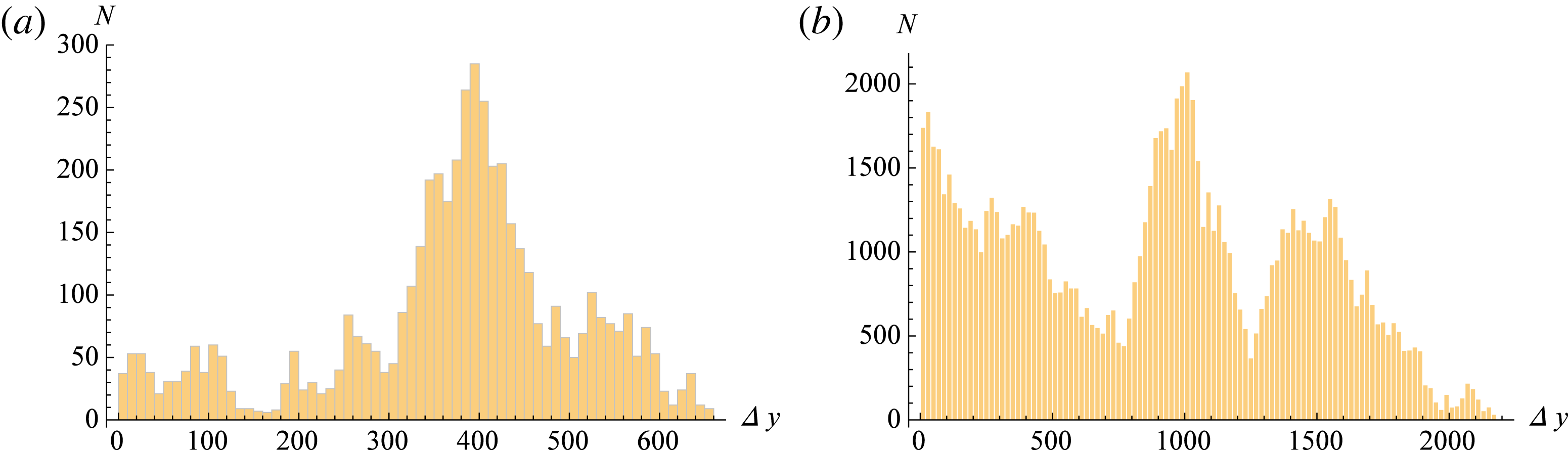
) which means that the particles experience some kind of acceleration when the trajectories are chaotic. Upon examination, it is found that there is a large contribution of large jumps whose size increases with time. This is apparent in the time evolution of the one-step displacements
 $|y_{n+1}-y_{n}|$
. As figure 11 shows, the mean step size grows with the number of iterations and the distribution peaks at very large steps. In the case of a single initial condition (one particle), numerical results indicate that the maximum step size scales as
 $|\unicode[STIX]{x0394}y|\sim t^{1/2}$
. It has to be mentioned that for cases with low or no chaos (small
 $A$
and
 $C$
), the transport is ballistic
 $\unicode[STIX]{x1D70E}_{y}\sim t^{2}$
, as it would be expected, since particles are simply transported by the parallel flow.
Histograms for the step length sizes
 $|y_{n+1}-y_{n}|$
in the chaotic regime with flow. There is a large contribution of very long jumps whose mean size strongly increases with time: (a) is for
 $N=5000$
iterations of the map while (b) is for
 $N=10^{5}$
.
(a) Variance of the
 $y$
displacements for thermal particles with
 $\unicode[STIX]{x1D70C}_{th}=1$
as function of time in log–log scale, showing the cubic scaling for
 $A=1$
(lower curve) and
 $A=20$
(upper curve). (b) Variance for
 $x$
for the same cases of (a). The regression fit is shown with dashed lines together with the corresponding equation.

The cubic scaling of the variance with time is preserved when the particle ensemble has a Maxwellian distribution of Larmor radii. This is shown in figure 12(a) for amplitudes
 $A=1$
and
 $A=20$
. In contrast to this atypical behaviour, the PDF of
 $y$
displacements exhibits a nearly normal distribution with kurtosis around 3 for small values of
 $\unicode[STIX]{x1D70C}_{th}$
. As
 $\unicode[STIX]{x1D70C}_{th}$
increases the PDF departs more and more from a Gaussian – the kurtosis increases. The long-tailed PDF for
 $\unicode[STIX]{x1D70C}_{th}=1$
is shown in figure 13. Notice the large extension spanned as a result of the very fast motions. On the other hand, the kurtosis is almost insensitive to the value of the flow parameter
 $C$
.
PDF in
 $y$
direction with background flow after 1000 time steps in log–linear scale for
 $\unicode[STIX]{x1D70C}_{th}=1$
showing non-Gaussian tails.

The accelerated transport observed for the displacement along the
 $y$
direction is due to the presence of flow combined with the chaotic transport. If the waves are removed (
 $A=0$
) the flow alone produces ballistic transport with no evidence of accelerated motion. On the other hand, the case with no flow analysed previously showed a diffusive transport. Thus, it is the superposition of both that adds up to produce the cubic scaling.
To explore the origin of the super-ballistic scaling note that from (4.5)–(4.6) it follows that
 $$\begin{eqnarray}\displaystyle \unicode[STIX]{x0394}x\equiv x^{n+1}-x^{n} & = & \displaystyle -\frac{A(\unicode[STIX]{x1D70C})}{2-C}[\sin (x_{-}^{n})-\sin (x_{+}^{n+1})]\end{eqnarray}$$
 $$\begin{eqnarray}\displaystyle \unicode[STIX]{x0394}y\equiv y^{n+1}-y^{n} & = & \displaystyle Cx^{n}-\frac{A(\unicode[STIX]{x1D70C})}{2-C}[(1-C)\sin (x_{-}^{n})+\sin (x_{+}^{n+1})].\end{eqnarray}$$
According to (4.9), the step size in
 $x$
is bounded by
 $|\unicode[STIX]{x0394}x|<2A(\unicode[STIX]{x1D70C})/(2-C)$
for
 $C<2$
. On the other hand, the displacement in
 $y$
,
 $\unicode[STIX]{x0394}y$
depends on the instantaneous
 $x$
position across the flow and it is in principle unbounded. This means that, as the particle goes farther from the origin with the usual random walk in
 $x$
, the jumps in
 $y$
get larger; it also has the random contribution but this is bounded to
 $\unicode[STIX]{x0394}y_{\text{max,rand}}=A(\unicode[STIX]{x1D70C})$
. This implies that there is a coupling of the motions across and along the flow. The chaotic displacements across the flow produced by the
 $x$
variation of the waves, transfer energy to the parallel motion.
It is interesting to ask whether the PDF for
 $y$
possesses a self-similar property. Given the cubic scaling one would expect a self-similarity equation of the type
 $$\begin{eqnarray}P(y,t)=\frac{1}{t^{3/2}}{\mathcal{G}}_{\unicode[STIX]{x1D70C}_{th}}\left(\frac{y}{t^{3/2}}\right).\end{eqnarray}$$
Since there is no diffusive transport we cannot associate a transport coefficient with this relation, so it only involves the time. Equation (4.11) was tested for the numerically obtained PDF and it was found that there is indeed this self-similar behaviour as shown in figure 14.
Self-similarity of the PDF in the
 $y$
-direction with flow for
 $\unicode[STIX]{x1D70C}_{th}=1,A=20$
and
 $C=0.7$
plotted for three times:
 $t=500,1000$
and 5000.

In the strongly chaotic regime, the displacements in the
 $x$
-direction exhibit diffusive scaling
 $\unicode[STIX]{x1D70E}_{x,th}\sim t$
as seen in figure 12(b). Thus, the same theoretical analysis made for the case with no background flow regarding the superposition of Gaussian PDFs for a thermal distribution of Larmor radii can be made in this case. As a result the PDF for a thermal population becomes non-Gaussian, although it is closer to a Gaussian for small
 $\unicode[STIX]{x1D70C}_{th}$
. However, the presence of flow in
 $y$
does affect the particle diffusion along
 $x$
. The diffusion coefficient obtained by the same procedure leading to (3.5) is now
 $$\begin{eqnarray}D(\unicode[STIX]{x1D70C})=\frac{1}{2(1-C/2)}(\unicode[STIX]{x03C0}AJ_{0}(\sqrt{2}\unicode[STIX]{x1D70C}))^{2}.\end{eqnarray}$$
This means that the radial diffusion in a toroidal device is increased by the shear flow. With this expression, the PDF for a thermal distribution of Larmor radii can be again calculated with (3.6) and the fit to the numerical results is also very good as seen in figure 15.


5 Conclusions
The
 $\boldsymbol{E}\times \boldsymbol{B}$
transport of test particles in the weak turbulence regime has been studied focusing on the effect of the finite Larmor radius. It was found that inclusion of the FLR changes the properties of transport, turning it less chaotic for
 $\unicode[STIX]{x1D70C}<x_{01}$
, where
 $x_{01}$
denotes the first zero of the Bessel function, and then the chaotic regions size oscillate as
 $\unicode[STIX]{x1D70C}$
grows. In the chaotic regime, corresponding to large wave amplitudes, the particle distribution function is Gaussian and the transport has a diffusive character, meaning that the squared width of the PDF increases linearly with time. When the ensemble of particles has a Maxwellian distribution of Larmor radii, the PDF becomes non-Gaussian. This is a novel result of this work and it can be explained by the fact that the superposition of two or more Gaussians of different widths is in general non-Gaussian. However, it is shown that the transport still has a diffusive scaling in time, with an effective diffusion coefficient that is a decreasing function of the thermal Larmor radius
 $\unicode[STIX]{x1D70C}_{th}$
. It is shown that the PDFs have a self-similar property that scales with time in the same way as diffusive processes. For small
 $\unicode[STIX]{x1D70C}_{th}$
the self-similarity function is Gaussian but for
 $\unicode[STIX]{x1D70C}_{th}>1$
this function is no longer Gaussian and exhibits tails of the type of a stretched exponential.
A consequence of this is that particle orbits with large Larmor radius, such as alpha particles, supra-thermal ions, or electrons associated with auxiliary heating, need a higher level of turbulence to become chaotic and show diffusive transport. Additionally, for the bulk thermal plasma, the effective diffusion is slower for high temperature, which is a desirable effect for having good confinement in burning plasmas. Also, the statistical distribution of particles departs from a normal distribution as the temperature increases. This implies that increasingly larger numbers of particles can reach farther locations as a result of FLR effects. The same results are obtained for motions in both
 $x$
and
 $y$
directions (i.e. radial and poloidal).
In the presence of a background flow with linear shear a symplectic mapping can be constructed with properties strikingly different from the mapping without flow. In particular, the chaotic transport in the direction of the flow becomes strongly non-diffusive: the spread of particle distribution scales as
 $\unicode[STIX]{x1D70E}_{y}\sim t^{3}$
. For wave amplitudes that still do not produce significant chaos the transport is ballistic
 $\unicode[STIX]{x1D70E}_{y}\sim t^{2}$
due to the convection produced by the flow. In contrast, the transport in the direction perpendicular to the flow is still diffusive. In this case, the same properties seen in the case with no flow are observed but with an increase in the diffusion due to the presence of flow. In particular, the non-Gaussian PDF resulting from a thermal distribution of FLRs, can be fit by a theoretical PDF produced by an effective diffusion coefficient.
The accelerated transport along the flow can be understood by the presence of an important contribution of long jumps that grow in size with time. These growing flights give rise to an accelerated motion parallel to the flow that is due to the coupling of chaotic transversal displacements with the ballistic transport along the flow. The two-dimensional waves have the effect of transferring energy from perpendicular to parallel motion. This is produced by the fact that the waves involve oscillations in both
 $x$
and
 $y$
directions. This is not an FLR effect but deserves further study.
However, regarding transport in toroidal plasmas, the accelerated transport does not have consequences for confinement since it is associated with the poloidal motion, which is also the direction of the flow. It just means that the poloidal spread of particles could be extremely fast. On the other hand, the radial transport has the diffusive properties found in the case with no flow except that the effect of a sheared poloidal rotation produces a faster diffusion.
Acknowledgements
This work was supported by DGAPA-UNAM PAPIIT project IN109115. N.K. is under a postdoc fellowship from CONACYT-SENER. D.dCN was sponsored by the Oak Ridge National Laboratory, managed by UT-Battelle, LLC, for the US Department of Energy under Contract No. DE-AC05- 00OR22725