1 Introduction
The phrase Grapheme-to-Phoneme (G2P) conversion is typically used to refer to the process of automatically generating pronunciation candidates for previously unseen words, or generating alternative pronunciations for known words.
G2P conversion is an important problem in both the areas of Automatic Speech Recognition and Text-to-Speech synthesis. In the case of Automatic Speech Recognition, the true vocabulary is often dynamic in nature. This means that new words, or new pronunciation candidates for existing words may need to be added to the system on a regular basis. Analogous problems arise in the case of Text-to-Speech synthesis. In both cases, building accurate G2P systems is typically both difficult and resource intensive. This difficulty derives from the fact that the letter-to-sound rules for natural spoken languages tend to be rife with special rules, inconsistencies and conflicts.
The Phonetisaurus G2P approach, which is the subject of this work, is another variation on the well-known joint multigram approach, and can be summarized in four steps. The first step is data preparation, which involves collecting a suitable pronunciation lexicon for training. This should include a list of known words and their corresponding pronunciations. The second step is to align the training lexicon, so as to approximate a mapping between the graphemes and phonemes in the lexicon. In the third step, the aligned corpus is utilized as the input to estimate a standard n-gram model, which is subsequently converted into a Weighted Finite-State Transducer (WFST). In the fourth and final step, pronunciations for previously unseen words are predicted by using weighted composition (Mohri, Pereira and Riley Reference Mohri, Pereira and Riley2002) to compute the intersection of the WFST representation of the target word and the joint n-gram model. The most likely pronunciation is determined by extracting the shortest-path through the combined machine. In depth discussion of each of these steps is provided in the following pages, starting with the pronunciation dictionary below.
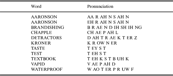
The pronunciation dictionary is typically constructed by expert linguists with experience in phonetics and phonology. Table 1 provides an example of several entries taken from the English-language, open source CMU pronunciation dictionary (Weide Reference Weide1998). Once a suitable training dictionary has been obtained or created, the next step towards training a G2P model is to align the graphemes and phonemes in the dictionary. In some cases, if the number of graphemes and phonemes is the same, as depicted in Table 2, this may be very simple.
Sample entries from the CMU pronunciation dictionary

Example alignments for ‘TEST → T EH S S T’ and ‘TASTE → T EY S T’, the latter of which requires a phonemic null

If the number of letters or phonemes does not match, it may be necessary to map letters or phonemes to a null symbol (ε) such as depicted in the second example from Table 2. In yet other instances, the number of graphemes and phonemes may be equal, but a one-to-one alignment may still be incorrect. An example of this situation is depicted on the left-hand side of Table 3.
Two example alignments for the word ‘TEXTBOOK → T EH K S T B UH K’. The first depicts a naive one-to-one alignment, the second an arguably more natural one-to-many alignment

In the TEXTBOOK example, graphemic and phonemic nulls could be used to produce a reasonable alignment, however it will almost certainly be more intuitive to instead permit one-to-many alignments between the grapheme and phoneme sequences. An example of this is depicted on the right-hand side of Table 3.
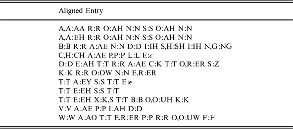
Section 3 describes a fully automated approach to acheive this sort of flexible alignment result utilizing the Expectation–Maximisation (EM) framework based on Yianilos and Ristad (Reference Ristad and Yianilos1998), and Jiampojamarn, Kondrak and Sherif (Reference Jiampojamarn, Kondrak and Sherif2007), and the WFST paradigm. The result of the alignment step then, is an aligned dictionary, as depicted in Table 4.
Results of aligning and reformatting the dictionary as a corpus of joint sequences. A ‘,’ indicates a one-to-many relationship, while ‘ε’ represents a null

The corpus of aligned joint sequences may be used directly to train a joint n-gram model. The first variation of this approach was proposed in Deligne, Yvon and Bimbot (Reference Deligne, Yvon and Bimbot1995) and various extensions and reformulations were proposed in Galescu and Allen (Reference Galescu and Allen2001), Caseiro and Trancoso (Reference Caseiro and Trancoso2002), Chen (Reference Chen2003), and Damper et al. (Reference Damper, Marchand, Adsett, Soonklang and Marsters2005). In Bisani and Ney (Reference Bisani and Ney2008), the authors propose another joint n-gram approach which combines the alignment, segmentation and model estimation procedures into one integrated framework based on maximum-likelihood EM. In the latter case, the authors also released their toolkit, Sequitur G2P (Bisani and Ney Reference Bisani and Ney2008). This has represented the gold standard in joint n-gram models for G2P for some time. A detailed and comprehensive review of further related work in this area is provided in Bisani and Ney (Reference Bisani and Ney2008). The central advantage of the joint n-gram approach is that is both fairly simple, and facilitates the use of research and tools developed by the Statistical Language Modeling community over the past twenty years.
The final step in most G2P solutions is the decoding step. Here, the model trained on the input corpus is utilized to produce pronunciation hypotheses for input words. The simplest-possible solution is to compose an Finite-State Acceptor (FSA) representation of the target word with the G2P model, and extract the shortest-path through the resulting lattice of pronunciations. This is the same basic approach described in Caseiro and Trancoso (Reference Caseiro and Trancoso2002). More sophisticated decoding procedures may also be applied, some of which are investigated in Section 6.
The main contribution of the current work can be summarised as the synthesis of the most effective components of previously proposed solutions in the literature, with a clear focus on achieving a balance between speed, accuracy and flexibility. In contrast to Bisani and Ney (Reference Bisani and Ney2008), the proposed toolkit opts to decouple the the alignment and joint multigram training stages, in the interest of increasing flexibility and reducing training time. This also makes it possible to compare several of the previously proposed approaches on an equal footing within the same framework. In contrast to earlier approaches (Galescu and Allen Reference Galescu and Allen2001; Caseiro and Transcoso Reference Caseiro and Trancoso2002; Chen Reference Chen2003; Damper et al. Reference Damper, Marchand, Adsett, Soonklang and Marsters2005), the current work provides support for training multiple-to-multiple, multiple-to-one / one-to-multiple alignments based on Jiampojamarn et al. (Reference Jiampojamarn, Kondrak and Sherif2007), as well as the ability to optionally utilise full alignment lattices for the purpose of training models based on fractional counts. In contrast to Galescu and Allen (Reference Galescu and Allen2001), Chen (Reference Chen2003), Damper et al. (Reference Damper, Marchand, Adsett, Soonklang and Marsters2005), and Bisani and Ney (Reference Bisani and Ney2008), the proposed toolkit employs the WFST framework in order to leverage the flexibiility and practical efficiency that this provides. It also implements a novel solution for the handling of back-off transitions in a joint n-gram model under the WFST framework. Finally, the toolkit provides native support for direct decoding of joint multigram-based Recurrent Neural Network Language Models, which represents a novel contribution in this area.
In the present work, we make the argument that the simple, decoupled G2P approach, based on the joint n-gram model has not yet been thoroughly exploited, and more generally that simple solutions can often provide surprisingly good results, sufficient to encourage their adoption in business and industry contexts, and to suggest avenues for further research in academic circles, especially in the case of large lexica.
The remainder of the paper is structured as follows. Section 2 introduces the WFST framework. Section 3 describes the alignment training procedure. Section 4 provides a synopsis of several Statistical Language Modeling techniques, WFST-based representations of G2P models, and descriptions of joint sequence RnnLMs for G2P conversion. Section 6 explains the model decoding processes for joint n-gram models and joint sequence RnnLMs. Section 7 provides a wide range of experiments using the proposed toolkit with n-gram based models, RnnLMs and ensemble methods. Section 8 provides final analysis, concluding remarks and possible directions for future work. Appendix A provides several basic examples of the available tools and their usage.
2 Weighted finite-state transducer preliminaries
The WFST framework has gained considerable popularity in the speech and NLP communities in recent years, in part because it provides a unified representational framework applicable to a wide range of different modeling and decoding techniques. Casting the G2P problem in the language of WFST provides us with access to a broad array of tools suitable for combination, optimization, training and decoding. Before proceeding further, we present a short introduction to the WFST framework including several important definitions and frequently used algorithms.
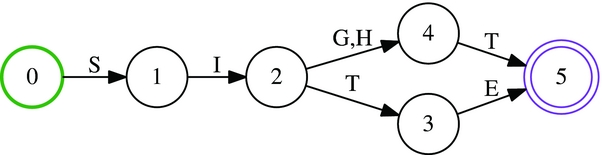
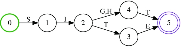
The starting point for the WFST framework is the familiar unweighted FSA. An example of an FSA describing possible graphemic representations of two words is depicted in Figure 1. Valid paths through the machine are defined as the concatenation of labels connecting the start state to one of the final states in the machine. In the case of Figure 1, there are two valid paths: one for ‘S I G,H T’, where the ‘G’ and ‘H’ are encoded as a cluster, and one that represents the homonym ‘S I T E’. The language represented by an FSA may be informally described as the set of valid paths that it encodes.
Example FSA depicting possible graphemic representations of the homonyms ‘SIGHT’ and ‘SITE’.
WFST extend the concept of the acceptor in two important ways. Namely, each arc or transition in the machine is extended to encode both a weight, and an output label, in addition to the input labels in the original FSA. The weight of a complete, valid path through the WFST is then determined by computing the product of the arc weights along the path. In a WFST, the output labels describe a second output language comprising again valid paths through the machine. The transducer itself then encodes a relation that maps paths from the input language to paths in the output language. Figure 2 illustrates another example relevant to the present work.
Example WFST mapping the homophones ‘SIGHT’ and ‘SITE’ to the pronunciation ‘S AY T’. The ‘ε’ symbol indicates null output.

In this example, the input language corresponds to the words ‘SIGHT’ and ‘SITE’, and the output language to the pronunciation ‘S AY T’. The ‘ε’ symbol indicates null-output.
Depending on the structure of the relation between the input and output languages, the transducer may produce a single output, or it may produce multiple different outputs for a given input. The example depicted in Figure 2 illustrates the former case. Both input orthographies, ‘S I G,H T’, and ‘S I T E’ will produce the same pronunciation output, ‘S AY T’. In the example, the weights of the two outputs are differentiated by their relative unigram frequency in English. In the event that an input path is not contained in the input language of the WFST, the transducer will not produce any output; rather it will reject the input. An FSA or Weighted Finite-State Acceptor (WFSA), on the other hand does not perform any mapping, but is said to represent, or accept a particular input language.
The WFST framework provides a wide range of known operations for manipulating machines. Many of these, including determinization, minimization and epsilon-removal, alter the structure of the WFST (e.g. the number of states, arcs, epsilon transitions, or the positions of weights and labels) without changing the language that the machine recognizes, the relation that it encodes or the associated total path weights. Others such as shortest-path and composition result in the creation of new machines.
All of these operations are underpinned by algebraic structures called semirings (Mohri Reference Mohri2002). Informally, these structures govern the way that path weights are computed by overloading the properties of the Plus (⊕), Times (⊗), Zero / annihilator (0) and One / identity (1) operators, as well as the set of values over which the operations are valid for a given semiring. The example in Figure 2 employs the familiar probability semiring. The current work relies primarily on two particular semirings: the log semiring and the tropical semiring, which are defined, along with the probability semiring in Table 5. The particular properties of each semiring influence its suitability for different applications.
Definition of the log and tropical semirings utilized in this work. Note that ⊕ log is defined as: x⊕ log y = −log(e − x + e − y )

In particular, the ⊕-operation for the log semiring indicates a summation of partial path weights. This makes it the right choice for the EM driven alignment algorithm described in Section 3. The ⊕-operation in the tropical semiring, by contrast, considers only the least costly partial path, making it suitable for the decoding stage described in Section 6, where the goal is to find the shortest-path through a lattice of pronunciation hypotheses. It is also suitable for using negative log probabilities, which matches with the language model representations employed throughout the current work. A detailed formal discussion of semirings is provided in Mohri (Reference Mohri2002).
There exists a wide variety of different algorithms to combine, manipulate and optimise WFSTs. It is beyond the scope of this work to discuss these algorithms in detail, however there are three in particular that bear mention, as they are utilised frequently by the proposed system. In the current work, the most fundamental of these operations is weighted composition, which is used to hierarchically cascade multiple WFSTs. Informally, given two input WFSTs, A and B, the composition algorithm works by matching paths in the output language of A with paths in the input language of B. The result of composition, C=A○B, is a new WFST, C where each input path u mapping to output path w in C is determined by matching input path u mapping to output path v in A, to input path v mapping to output path w in B. The weights of paths in the composition result, C are determined by computing the ⊗-product of the corresponding paths in A and B, according to the specified semiring (Mohri et al. Reference Mohri, Pereira and Riley2002). The process may be applied to an acceptor by simply mirroring the input labels to output labels to produce an equivalent transducer.
Other operations ultized in the current work include projection, which is used to transform a WFST into a WFSA representing just the input language or just the output language of the original machine. In the current work, this operation is utilized to obtain pronunciation lattices during the decoding stage. The shortest distance operation, which is used to compute the shortest distance from the start state to every other state, is utilized by the EM-alignment stage in the current work. Finally, the shortest-path operation, which is used to compute the shortest-path through the input machine starting from the start to a final state, is utilized during both the alignment and decoding stages. Formal definitions and in-depth discussions of these algorithms and many more can be found in Mohri et al. (Reference Mohri, Pereira and Riley2002) and Mohri (Reference Mohri2002). Similarly, robust open-source implementations and examples of these algorithms are provided in the OpenFst toolkit (Allauzen et al. Reference Allauzen, Riley, Schalkwyk, Wojciech and Mohri2007).
3 Grapheme-to-Phoneme alignment
3.1 Algorithm motivation and overview
The typical first step in training a G2P system involves aligning the corresponding grapheme and phoneme sequences in the input training dictionary. The approach adopted in this work is based on the EM driven multiple-to-multiple alignment algorithm proposed in Jiampojamarn et al. (Reference Jiampojamarn, Kondrak and Sherif2007) and extended in Jiampojamarn and Kondrak (Reference Jiampojamarn and Kondrak2010). This algorithm is capable of learning complex G↔P relationships like PH → /F/, and represents an improvement over earlier one-to-one stochastic alignment algorithms such as that introduced in Yianilos and Ristad (Reference Ristad and Yianilos1998). This approach is also similar to that proposed in Deligne et al. (Reference Deligne, Yvon and Bimbot1995), but appears to have been independently discovered.
The alignment algorithm utilized in this work includes three minor modifications to the work of Jiampojamarn et al. (Reference Jiampojamarn, Kondrak and Sherif2007): (1) A constraint is imposed such that, in addition to one-to-one relationships, only multiple-to-one and one-to-multiple relationships are considered during training. (2) During initialization, a joint alignment lattice is constructed for each input entry, and any unconnected arcs are deleted. (3) All arcs, including deletions and insertions are initialized to, and constrained to maintain a non-zero weight. These minor modifications appear to result in a small but consistent improvement in terms of Word Error Rate (WER) on G2P tasks. Finally, the training procedure is cast in the WFST framework, which admits a very concise representation and implementation of the algorithm.
The first step in the WFST-based version is to generate an alignment lattice for each word-pronunciation pair, based on the user-supplied input parameters.
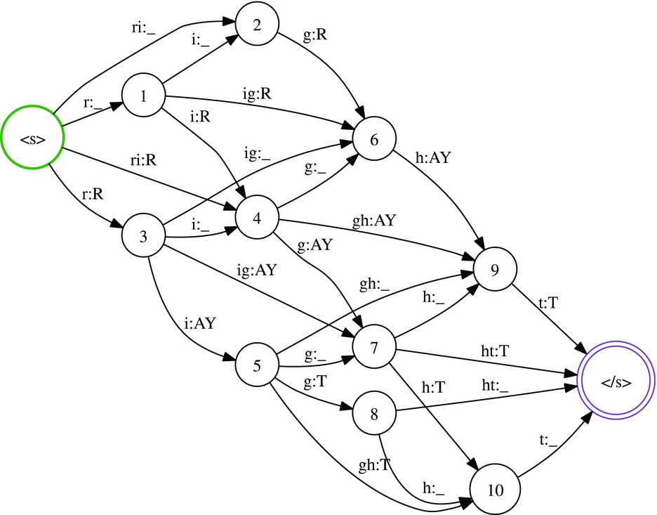
Figure 3 illustrates an example FST that encodes all permissible alignments for the word-pronunciation pair ‘RIGHT’, ‘R AY T’, given the constraints that (a) the maximum length for a grapheme subsequence is two, (b) the maximum phoneme subsequence length is and deletions are permitted only on the phoneme side.
Example alignment lattice for the word↔pronunciation pair ‘RIGHT’, ‘R AY T’ illustrating all possible alignments between the graphemes and phonemes in the given entry. In this example, the maximum length for a grapheme subsequence has been set to two, the maximum phoneme subsequence length to one, and deletions were permitted only on the phoneme side.
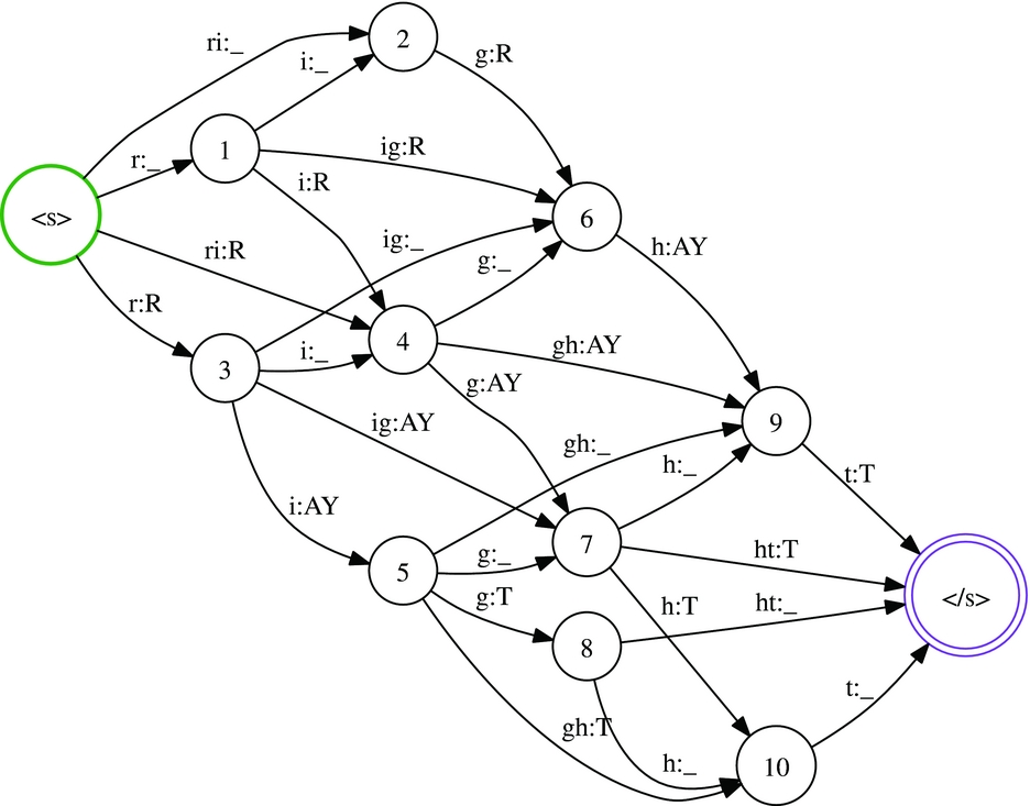
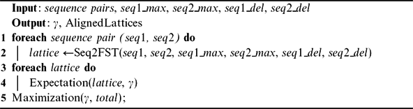
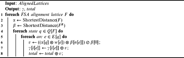
Once an alignment lattice has been generated for each entry in the training dictionary, the EM training procedure is initialized by setting all possible grapheme–phoneme alignment pairs to uniform probability. Next, the set of alignment lattices are passed to the expectation function. The WFST-based version of the algorithm is summarized in Algorithm 1. The procedure is initialized with a lexicon and a set of user-supplied constraints. Lines 1–2 process each word/pronunciation pair and generate a WFST lattice like the example depicted in Figure 3. The EM steps described in lines 3–5 are then repeated until the algorithm either converges, or until a prespecified maximum number of iterations is reached. The expectation step is described in Algorithm 2; this is fundamentally the same as the approach described in Jiampojamarn et al. (Reference Jiampojamarn, Kondrak and Sherif2007), with the exception that it has been reformulated to take advantage of the WFST framework.
EM-driven M2One/One2M

Expectation step

Maximization step

Here, the traditional forward and backward steps are implemented in lines 2–3 using the shortest-distance algorithm. This is computed in the log semiring because we wish to compute the sum of all paths leading into each state. Next, the alpha and beta values are used to compute the arc posteriors according to the standard formula,
 $\gamma _{ij}=\frac{\alpha _{i}\cdot w_{ij}\cdot \beta _{j}}{\beta _{0}}$
. Here, α
i
represents the shortest distance in the log semiring from the start state to state i, and is represented by α[q] on line 6 in Algorithm 2. Similarly, β
j
represents the shortest distance in the log semiring from the final state to state j and is represented by β[n[e]] on line 6. Finally, wij
represents the original weight for the arc connecting states i and j, and corresponds to w[e] on line 6. Line 7 sums the arc posteriors for each possible grapheme–phoneme correspondence over the set of alignment lattices, and Line 8 keeps a running total, which is utilized to normalize the arc weights during the maximization step.
The maximization step in this case corresponds to normalizing the partial counts that were accumulated during the expectation step. This is outlined in 3. It is possible to perform a conditional maximization using the FST formalism, in which case the partial counts are normalized on a per-grapheme or per-phoneme basis, or jointly in which case the partial counts are normalised over the complete set of grapheme–phoneme correspondences (Shu and Hetherington Reference Shu and Hetherington2002).
In the present work, we focus on joint maximization, which reduces to normalizing the partial counts for each correspondence using the final value of total returned at the end of the expectation step. Finally, the lattice arc weights are reset to the new values and the expectation step is called again. This process terminates either when it reaches the maximum number of iterations, or when the change between the current iteration and previous iteration is less than some prespecified threshold.
Once the EM training process has successfully terminated, the most likely alignment can be extracted by mapping each alignment lattice to the tropical semiring and running the shortest-path algorithm (Mohri Reference Mohri2002). This is necessary as the Shortest-path algorithms require that the associated semiring have the path property, and be right distributive (Mohri Reference Mohri2002). The alignments may be printed out to create a corpus such as that depicted in Table 4. The n-best alignments may also be extracted, however in this case the resulting fractional counts will complicate downstream model training. It is similarly possible to utilize the full alignment lattices however, in practice this tends to be extremely resource intensive, even for small corpora, and results in little gain in terms of word or phoneme accuracy.
4 Joint sequence n-gram models for G2P conversion
4.1 Introduction
Once the input pronunciation dictionary has been successfully aligned, the next step is to train a model that can be used to produce pronunciation hypotheses for previously unseen words. In this work, we focus exclusively on joint n-gram models, which continue to enjoy considerable success in the area of G2P conversion. The training approach in the proposed system is identical to that used for modeling word sequences except for the fact that the ‘words’ are joint G↔P chunks learned during the alignment process. This means that any standard statistical language modeling toolkit may be used to train a joint n-gram model for the proposed system.
In the current work, we focus on two popular smoothing approaches: Witten–Bell smoothing (Bell, Cleary and Witten Reference Bell, Cleary and Witten1990; Witten and Bell Reference Witten and Bell1991), and Kneser–Ney smoothing (Kneser and Ney Reference Kneser and Ney1995). Kneser–Ney and its variations consistently outperform Witten–Bell smoothing, however Witten–Bell smoothing generalizes naturally to fractional counts. This means it can be used with lattices and n-best results such as those produced during the G2P alignment process.
In addition to standard n-gram language modeling techniques, maximum-entropy language models have been shown to perform competitively in G2P tasks (Chen Reference Chen2003). The maximum-entropy formulation admits a direct conversion to ARPA-format without loss of information (Wu Reference Wu2002), and an open-source implementation of this algorithm, which focuses on n-gram features, can be found in the SRILM toolkit (Stolcke Reference Stolcke2002; Alumäe and Kurimo Reference Alumäe and Kurimo2010). Evaluations with maximum-entropy joint n-gram models are also provided in Section 7.2.
4.2 WFSA and WFST representations
In order to utilize a joint n-gram model in the proposed WFST-based G2P system, it is first necessary to convert the model from the standard ARPA format representation to an equivalent transducer. Several algorithms and implementations suitable for representing a standard n-gram language model as an equivalent WFSA are proposed in Allauzen, Mohri and Roark (Reference Allauzen, Mohri and Roark2003), Roark et al. (Reference Roark, Sproat, Allauzen, Riley, Sorensen and Tai2012).
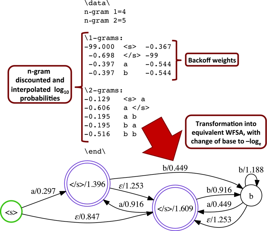
An example of the result of converting a standard ARPA format n-gram model to WFSA format is depicted in Figure 4.
Example transforming an ARPA format statistical language model into equivalent WFSA format. This is a bi-gram model trained on a small toy corpus, using interpolated Kneser–Ney smoothing. Note that the conventional base for the ARPA format and the tropical semiring differ, and that the sentence-begin (<s>) and sentence-end (</s>) tags are given special treatment during model estimation.
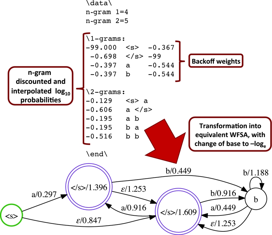
In this representation, both the sentence-begin (<s>) and sentence-end (</s>) tokens are implicitly represented by the start and final states in the WFSA, but are not explicitly represented in the graph. As noted in Roark et al. (Reference Roark, Sproat, Allauzen, Riley, Sorensen and Tai2012), this representation is more concise and also allows the sentence-begin and sentence-end tokens to be specified at run-time. It is also worth noting here that the ARPA format traditionally represents n-gram probabilities in log 10 format, while the WFST framework conventionally employs − loge .
Note also that the <s> and </s> tokens are given special treatment during the model estimation phase. Each sentence is implicitly understood to begin with <s> and this token is not counted as a unigram event, although it is included in the model vocabulary. Similarly, the </s> token is implicitly defined as marking the end of a sentence, and thus has no back-off weight associated with it.
In the case of a joint n-gram model, the model must be represented not as an acceptor but as a transducer. Here, the joint tokens learned during the alignment process are reseparated. Input labels represent graphemes, while the output labels represent phonemes.
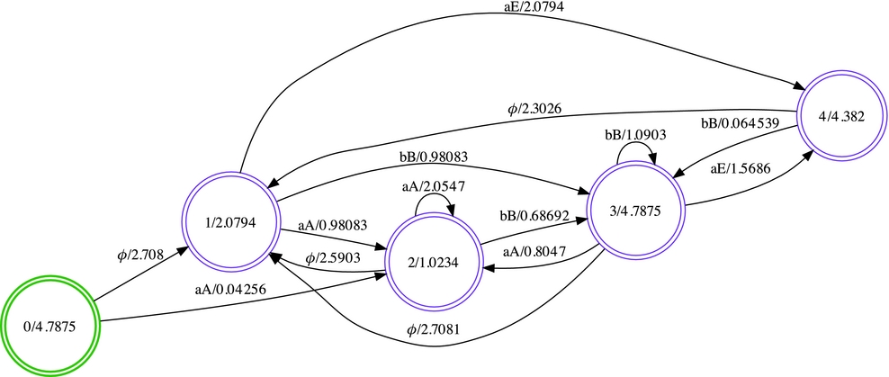
This final step will allow downstream composition with novel input words, which are represented as unweighted acceptors. The default approach in Phonetisaurus utilizes standard epsilon transitions to represent back-off weights. Strictly speaking, this is not correct as it means that the back-off arc will be traversed regardless of whether or not a higher-order n-gram exists. In Allauzen et al. (Reference Allauzen, Mohri and Roark2003), an alternative solution is proposed using special failure arcs, which are only traversed when no other valid match is found. Two algorithms for adapting this approach to joint n-gram models are proposed in Novak, Minematsu and Hirose (Reference Novak, Minematsu and Hirose2013). These are summarized in Section 4.3 and implementations are provided in the proposed toolkit.
4.3 Failure transitions and joint n-gram models
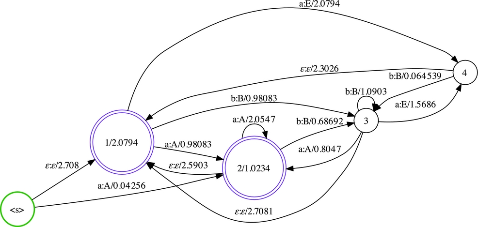
The starting point for model transformation is to utilize ε-based back-off transitions. This is an approximate solution which works well in practice, but is both inexact, and tends to generate redundant paths which differ only in the placement of back-off transitions. An example of this starting point is depicted in Figure 5.
G2P n-gram model representation using ε back-off transitions.
Utilizing the ϕ-based method from Allauzen et al. (Reference Allauzen, Mohri and Roark2003) will largely produce incorrect results.
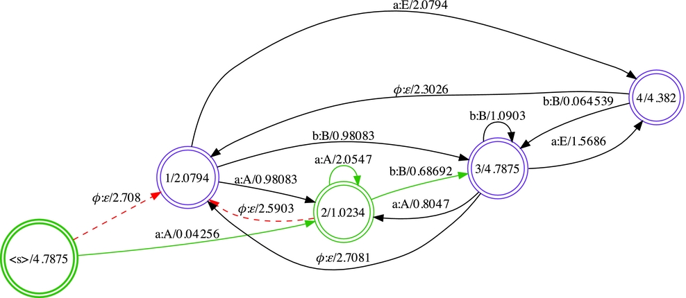
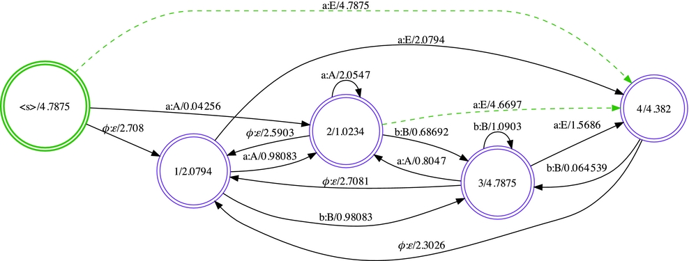
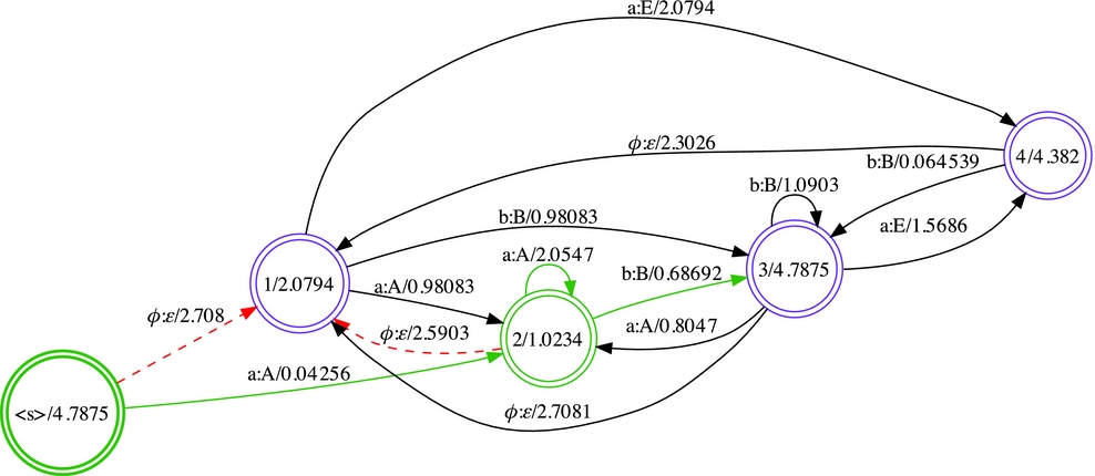
A ϕ-based equivalent of Figure 5, is depicted in Figure 6. The green arcs depict the result of composing the word ‘aab’ with the model. This produces the hypothesis ‘AAB’, but the hypotheses, ‘EAB’, ‘EEB’, ‘AEB’ are ignored because the failure arc is not traversed. Two solutions to this problem follow.
Illustration of attempting to compose linear FSA ‘aab’ with a WFST representation of a joint n-gram model while interpreting back-off transitions as ϕ arcs. Green arrows indicate arcs that are traversed, while red, dashed arcs indicate arcs that are incorrectly ignored.
4.3.1 Encode-based solution
The first solution is to encode the input and output labels in the joint n-gram model, creating an acceptor. The same is done with the input test word, taking care to generate all possible grapheme–phoneme alignments that were learned during the training phase. Once this has been done, the standard ϕ-based approach from Allauzen et al. (Reference Allauzen, Mohri and Roark2003) can be used. An example illustrating this solution is depicted in Figure 7.
Example of ϕ-enabled, WFSA version of the G2P joint n-gram model where the input–output labels have been encoded.

4.3.2 Transition modification solution
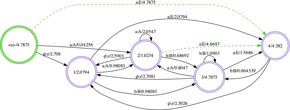
The second solution augments the original algorithm (Allauzen et al. Reference Allauzen, Mohri and Roark2003), by inspecting the input label of each outgoing arc, and adding new transitions wherever necessary in order to guarantee that all valid grapheme–phoneme correspondences are supported in the final result.

Listing 1: Python pseudocode for the fsa_phi algorithm. add_explicit_arc() iterates across the back-off arcs until an arc with the missing il/ol pair is found. A new arc is created connecting the original state to the destination state, and the weight is set to the accumulated back-off cost.
An example of the second solution is shown in Figure 8. New transitions have been added to guarantee that all valid pronunciation hypotheses will be considered during composition.
Example of modified ϕ-enabled WFST version of the G2P joint n-gram model. Explicit transitions have been added for each missing grapheme–phoneme correspondence at each state. Transitions added by the algorithm are dashed and green.
4.3.3 Comparison of methods
In practice, the three methods summarized above produce equivalent PER/WER results. The two ϕ-transition based methods produce the exact same results, while the standard ε based method produces slight variation but no consistent improvement or degradation in accuracy.
In terms of run times, the ε based solution is the fastest for one-best, but slows down dramatically when generating n-best. This is due to the fact that there are often multiple variations of each pronunciation hypothesis, which differ only in the placement of back-off transitions. In the case of n-best, it is more efficient to employ the fsa_phi or fst_phi solution instead. Further details regarding the performance and accuracy characteristics for the three methods mentioned above can be found in Novak, Minematsu and Hirose (Reference Novak, Minematsu and Hirose2013).
5 Joint sequence RnnLMs for G2P conversion
5.1 Introduction
Recurrent Neural Network Language Models have recently enjoyed a resurgence in popularity in the context of Automatic Speech Recognition applications (Mikolov et al. Reference Mikolov, Karafiat, Burget, Černocký and Khundanpur2010). In another recent publication (Novak et al. Reference Novak, Dixon, Minematsu, Hirose, Horie and Kashioka2012), we investigated the applicability of this approach to G2P conversion with joint sequence models, by providing rescoring support for the rnnlm toolkit (Mikolov et al. Reference Mikolov, Kombrink, Anoop, Burget and Černocký2011).
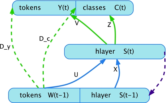
Here, we provide a brief description of the RnnLM architecture, and introduce a series of recommendations that serve to optimize the approach for G2P conversion. Finally, we provide a mechanism and implementation for performing efficient direct decoding using a joint token G2P RnnLM. The full architecture of the RnnLM is depicted in Figure 9.
Full RnnLM architecture utilized for G2P conversion.

The network is represented using specially partitioned input, hidden and output layers. These have corresponding weight matrices U and X, which map between the input and hidden layers; V and Z, which map between the hidden and output layers; and D y and D c , which map directly between the input and output layers (Mikolov Reference Mikolov2012). The network is trained using the backpropagation through time (BPTT) algorithm, with the goal of maximizing the likelihood of the training data.
The input layer consists of an indexed vector representing the vocabulary, which corresponds to the set of joint multigrams in the G2P case. This is augmented with a copy of the hidden layer activations from the previous time step. This two-component input layer feeds into the hidden layer. The hidden layer then feeds separately into an output layer, which is again split into two components. The first component partitions the vocabulary into disjoint classes based on unigram frequency. The second represents the class conditional probabilities for the vocabulary. The goal of this partitioning is primarily to speed up computation. Finally, the direct connections between the input and output layers simulate maximum-entropy features based on n-gram histories. In practice, the n-gram histories are hashed into a fixed size array. This serves to keep the number of direct-connections tractable, while at the same time effect a pruning process where more frequently occurring features are favored when collisions occur. Output values for the various layers are then computed as described in Mikolov (Reference Mikolov2012).
5.2 RnnLM training caveats for G2P conversion
In practice, training efficient, effective and accurate RnnLMs requires the use of considerable tuning both at the implementation and training levels. Recommendations for efficient training, as well as an implementation are provided in Mikolov et al. (Reference Mikolov, Kombrink, Anoop, Burget and Černocký2011), and Mikolov (Reference Mikolov2012), however these focus on applying the work to textual data, specifically in the area of Large Vocabulary Speech Recognition. In the case of G2P conversion, there are a couple additional concerns.
First, it is important to always treat each dictionary entry independently during training. By default, the RnnLM toolkit treats the input text as a continuous stream of tokens. In this situation, BPTT training is conducted across sentence boundaries. This makes sense for Large Vocabulary Speech Recognition tasks, but it is ill suited to pronunciation dictionaries.
Second, it is essential that the training corpus be provided in randomized order. Pronunciation dictionaries are typically provided in lexicographically sorted order. If the sorted dictionary is utilized directly during training then the online or mini-batch variants of gradient descent have a strong tendency to find a poor local minimum.
Phonetisaurus also provides a further set of RnnLM-based examples suitable for training high-quality joint sequence RnnLMs for G2P conversion.
6 G2P decoding in the WFST framework
6.1 Introduction
The default decoder used in the proposed WFST-based approach, and implemented in the proposed toolkit, is similar to that described in Caseiro and Trancoso (Reference Caseiro and Trancoso2002). This version of the decoding process is summarized in Equation (1),
 $$\begin{equation}
p_{best} = shortestpath(project_{o}(w\circ M) ).
\end{equation}$$
In the proposed approach, it is necessary to make several modifications to the input FSA. The multiple-to-multiple EM alignment process may produce grapheme and phoneme tokens that consist of a cluster of two or more symbols from the original grapheme or phoneme alphabets. If these clustered tokens are not accounted for when constructing the input FSA, any examples of these clusters in the joint n-gram model will be ignored during composition. There are two possible solutions to this problem. One solution is to create a single-state FST that maps any longer grapheme subsequences to a single cluster label, while passing through single graphemes, then compose it with the linear FSA w, and apply projecto ( · ) to the result. The alternative is to build the combined FSA explicitly. The WFST-based solution is arguably more flexible, however it is also somewhat more computationally intensive. Implementations for both approaches are provided in the proposed toolkit.
One final potential pitfall needs to be mentioned. If the data utilized to train the alignments is limited and certain subsequences occur only in clustered contexts, this might result in an aligned corpus that does not contain examples of every individual grapheme in isolation. In order to ensure that creation of the linear FSA representation succeeds, it is necessary to add all individual graphemes to the input symbols table, even if some do not appear in the aligned corpus.
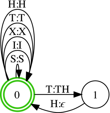
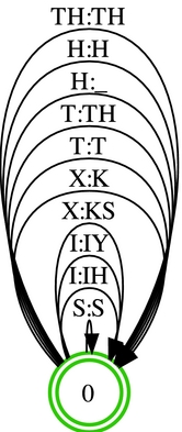
An example of the component machines and conversion process for the input word ‘SIXTH’ is illustrated in Figures 10–14. Figure 10 depicts a linear FSA w, representing the word ‘SIXTH’. Figure 11 depicts a flower transducer C (Kempe Reference Kempe2001), that may be used to augment w with cluster arcs. Figure 13 depicts the result of computing RmEps(Projecto (w○C)). Figure 12 depicts a single state flower transducer that may be used to map G2P correspondences. Here, the ‘_’ indicates that the grapheme ‘H’ may optionally map to a null phoneme output. Figure 14 depicts the result of computing RmEps(Min(Det(w′○F))). This final result is an FST w′′, that encodes all possible paths through the joint n-gram model, based on the set of G↔P correspondences learned during the alignment process. Note that the optimization routines are not strictly necessary at this stage, and may require label-encoding to succeed in the general case.
Example result of converting the word ‘SIXTH’ to an equivalent linear FSA w. This example does not utilize insertion self-loops.

Flower transducer C, suitable for expanding clusters.

Flower transducer F, suitable for mapping G↔P correspondences.

FSA w′, result of computing RmEps(Projecto (w○C)). This is utilized to expand grapheme clusters learned during the alignment process. It is necessary in order to guarantee that all valid pronunciation hypotheses can be generated.

FST w′′, result of computing RmEps(Min(Det(w′○F))).

If only one-to-one correspondences are permitted during the alignment process, then it is sufficient to simply use the linear FSA w. If clusters are permitted, then it will be necessary to utilize w′. If one prefers to interpret the back-off transitions in M as ϕ-transitions then it will be necessary to utilize w′′. The latter case also requires modifying the input model according to one of the approaches described in 4.3.
If phoneme insertions are permitted, then it is also necessary to augment w with an insertion self-loop at each state, or to use one of the more sophisticated techniques described earlier.
6.2 Direct decoding with joint sequence RnnLMs
The structure of the joint sequence RnnLMs requires a specialized decoding approach (Auli et al. Reference Auli, Galley, Quirk and Zweig2013). We have implemented an efficient decoder suitable for direct decoding of joint sequence RnnLMs, and released it as part of the Phonetisaurus toolkit. The decoder uses a strategy similar to the phrase-based decoder described in Auli et al. (Reference Auli, Galley, Quirk and Zweig2013). First, the input word is converted into an equivalent FSA, in the same manner as the n-gram based decoder. Next, a vector of priority queues is initialized, one for each state in the linear input FSA. The input network is a directed, linear, acyclic acceptor, thus is it sufficient to cycle once through the list of states. The first priority queue in the vector is initialized with an empty token. Next, a token is created for each grapheme–phoneme combination leaving from the start state. Each token tracks the history, hidden-layer activations, total score, current label score and a pointer to the parent token. The score for the current arc is computed using the feed-forward formula described in Mikolov (Reference Mikolov2012). The tokens are inserted into the priority queue associated with the destination state of the current input arc, subject to a possible beam constraint. The decoding process then proceeds to the next state in the input FSA and begins exploring the set of tokens associated with the appropriate priority queue, in order of least total cost. The algorithm terminates when a final state is encountered, and returns the best hypothesis. In practice, it is only necessary to explore the first 15–20 tokens in the priority queues associated with each state, thus the overall decoding process, while slower, is still competitive with the joint n-gram solution, and does not suffer from an exponential explosion in the state space. The algorithm extends naturally to N-best results, and the implementation is released as a companion module to Phonetisaurus.
7 Experiments
In this section, we present experimental results covering alignment, standard n-gram models, direct decoding with joint sequence RnnLMs, model combination and finally summarize the results of independent third-party experiments.
7.1 Alignment experiments
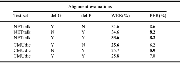
Here, we present a short series of alignment evaluations using the proposed toolkit, exploring several basic parameters. These include whether or not deletions are allowed in the grapheme or phoneme sequences. The maximum subsequence length is fixed to two, and a joint maximization function is used. These settings were chosen after replicating the recommendations from Jiampojamarn et al. (Reference Jiampojamarn, Kondrak and Sherif2007).
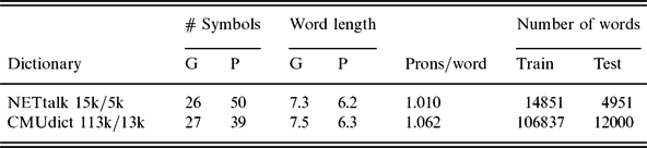
Here, two popular English language pronunciation dictionaries are considered, the NETtalk dictionary (Sejnowski and Rosenberg Reference Sejnowski and Rosenberg1993) and the CMUdict dictionary (Weide Reference Weide1998). These two dictionaries are utilized throughout this work, primarily because they are open-source and available for download via the web. Furthermore, widely used training/testing splits exist for both of these dictionaries, making it straightforward to replicate and compare experiments from previous work. Details on the NETtalk 15k/5k split and the CMUdict 113k/13k split are reproduced from Bisani and Ney (Reference Bisani and Ney2008) in Table 6. These are faithful replications of the splits from Chen (Reference Chen2003).
Overview of the NETtalk (Sejnowski and Rosenberg Reference Sejnowski and Rosenberg1993), and CMUdict (Weide Reference Weide1998) dictionary splits from Bisani and Ney (Reference Bisani and Ney2008)

The results of applying different alignment parameters to these two test sets are displayed in Table 7. The purpose of these experiments was to determine what, if any impact the choice of alignment parameters might have on downstream accuracy of the G2P system. In order to focus on the impact of the alignment process, the parameters for the joint n-gram model were fixed. In both cases, the Google OpenGrm (Roark et al. Reference Roark, Sproat, Allauzen, Riley, Sorensen and Tai2012) toolkit was used to train the joint n-gram model, using standard Kneser–Ney smoothing. For the comparatively small NETtalk dataset, the order of the n-gram model was set to seven, and for the CMUdict to thirteen. Ultimately, the results indicate that the choice of deletion parameters has little impact on the downstream accuracy, however allowing deletions on both sides increases the computational complexity of the alignment algorithm. As a result, the choice was made to permit deletions on the grapheme side but not the phoneme side as the default configuration for further experiments. In Section 4, further discussion of language model tuning for G2P will illustrate several simple ways to further improve these results.
Impact of allowing deletions (del G,del P), in the alignment lattice. Here, WER refers to Word Error Rate and PER to Phoneme Error Rate for the NETtalk 15k/5k split and the CMUdic 113k/13k split

The del G and del P parameters indicate whether deletions were permitted in the grapheme and phoneme sequences respectively. A joint maximization was performed over the full set of joint G↔P correspondences. WER refers to Word Error Rate, which is C(Pc
)/C(W), the percentage of exactly correct pronunciations, C(Pc
), in full set of unique test words, C(W). In the event that a test word has multiple correct pronunciations, the word is counted exactly once towards the total, and a pronunciation hypothesis is counted correct if it matches one of the acceptable variants. PER corresponds to Phoneme Error Rate. This is equivalent to WER for speech recognition, and is computed based on the Levenshtein distance,
 $PER = 1.0 - \frac{N-(S+D+I)}{N}$
where N refers to the number of phonemes in the reference pronunciation, and S, D and I refer to substitutions, deletions, and insertions respectively.
7.2 Smoothing experiments
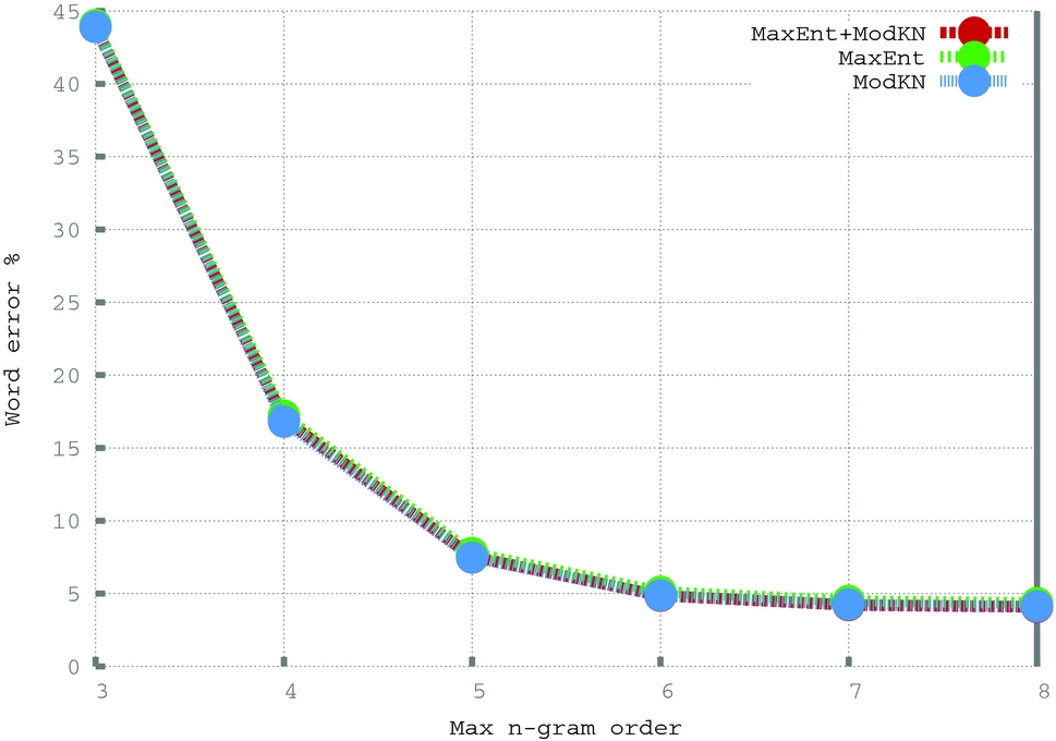
Here, we present a series of evaluations looking at the effect of different n-gram orders and smoothing techniques. In these experiments, the language models were all trained utilizing either the Google OpenGrm tools (Roark et al. Reference Roark, Sproat, Allauzen, Riley, Sorensen and Tai2012) or SRILM (Stolcke Reference Stolcke2002). In particular, the system was evaluated using the Modified Kneser–Ney, Absolute and Witten–Bell smoothing techniques for n-gram orders 3–8 using the CMU dataset. In addition, the SRILM toolkit with the maximum-entropy extension was utilized to train a parallel maximum-entropy n-gram model, which was then interpolated with the Modified Kneser–Ney model at each n-gram order. Empirically, this last combination provides the best results. The WER versus n-gram order results for these experiments are plotted in Figure 15. These results indicate that accuracy gains plateau around n = 6. Independent results for several larger datasets, which are reproduced in Section 7.6 indicate that this plateau point is fairly consistent, at least for European languages.
Plot of WER vs. n-gram order for several different smoothing algorithms on the CMU dataset.

In order to illustrate the scalability of the proposed toolkit and approach, we also conducted experiments using a much larger, proprietary Russian language lexicon, which is currently in use at Yandex as a component of their Automatic Speech Recognition system. The Russian language has a comparatively regular G2P relationship (Stüker and Schultz Reference Stüker and Schultz2004), however the lexicon also contains a wide variety of proper names, abbreviations and acronyms. Details for this lexicon are presented in Table 8.
Overview of the Yandex Russian training and testing lexica. Note: this is the first report on this particular dataset

The training set for this lexicon contains roughly 1.7 million entries, while the test set contains approximately 188 thousand words. To the best of our knowledge, this is the largest test set for which any G2P results have previously been reported. This is also the first report on this particular dataset. Unfortunately, no other available open-source tools were efficient enough to scale to this task, so we do not have a comparison for this benchmark. The alignment and n-gram model training processes for this experiment utilized exactly the same parameters as were applied for the CMU evaluations. Based on the results from the CMU experiments, we decided to only train Modified Kneser–Ney, maximum-entropy, and an interpolated variant of the two for this experiment. The results for this experiment are depicted in Figure 16.
Plot of WER vs. n-gram order for several different smoothing algorithms on the Yandex-ru dataset.
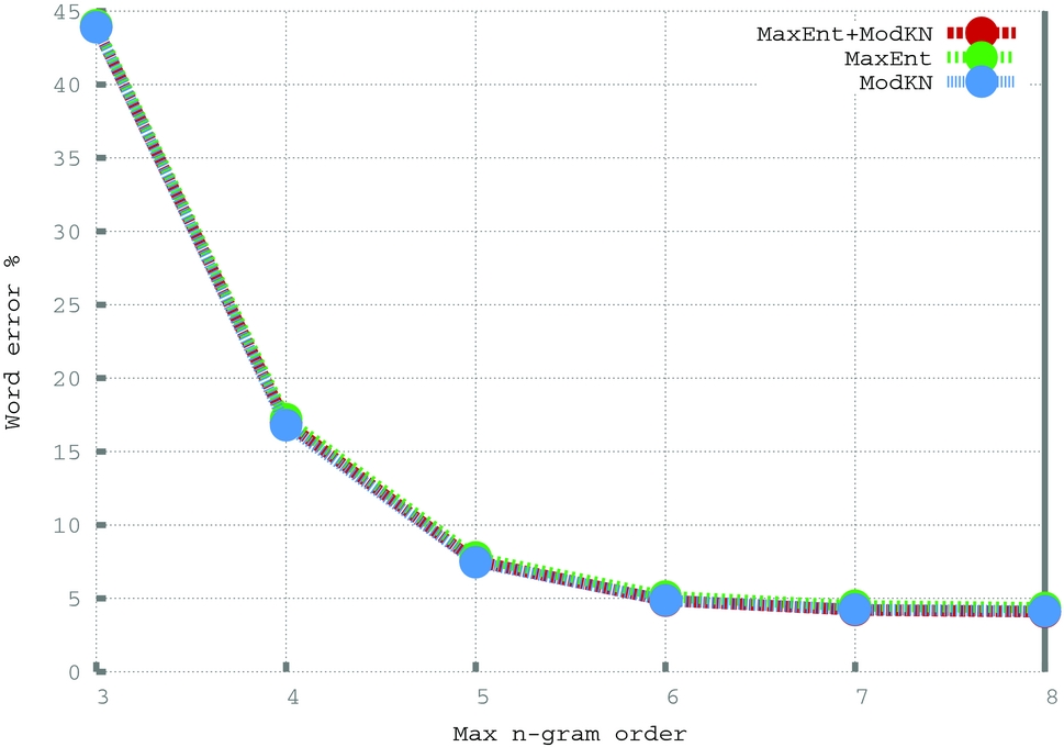
In this case, the accuracy gains again plateau around n = 6. The minimum WER and PER achieved were 4.09 per cent and 0.64 per cent for the interpolated MaxEnt + ModKN system, however there was not a significant WER difference in this case between the three evaluated systems. In terms of training time, it required approximately three hours to perform the alignment step, five minutes to train the eight-gram Kneser–Ney model, and fifteen minutes to train the eight-gram maximum-entropy model. Decoding the test set required approximately eight minutes.
7.3 N-best alignments and fractional counts
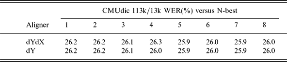
The preceding experiments all focused on training joint n-gram models based on the one-best alignment for each word in the training corpus, however as mentioned in Section 3, phonetisaurus-align is also capable of outputting n-best alignments or full alignment lattices. In practice, most standard language modeling techniques focus on integral counts, and do not naturally generalize to the sort of fractional counts that are encoded in a lattice. The Witten–Bell smoothing technique does however generalize naturally to fractional counts and we present results looking at oracle n-best results using this technique and various values of n in Table 9. The purpose of these experiments was to ascertain what, if any potential there might be in further investigating system combination and reranking techniques.
WER% for the CMUdic 113k/13k split using N-best alignments with 1 ⩽ N ⩽ 8, Witten–Bell smoothing, and n-gram order seven. Here, dY means deletions were allowed on the output side only

The results from these experiments indicate that there is minor room for further improvement using the n-best alignments, assuming a effective reranking methodology, but that this tapers off around N = 5. Using the full lattices is also an option, however computing counts in this case quickly becomes very expensive, and the return in terms of accuracy improvements is likely to minimal or non-existent. Although the n-best results potentially provides minor accuracy improvements within Witten–Bell smoothing, even at N = 5 Modified Kneser–Ney using one-best alignments is still superior. The standard formulation for Kneser–Ney smoothing is based on integral counts, and thus cannot be directly applied to lattices, however in recent years, two generalizations to fractional counts have been proposed (Bisani and Ney Reference Bisani and Ney2008; Tam Reference Tam2009).
The approach proposed in Tam (Reference Tam2009) is compared with Witten–Bell using bigram models in the context of latent semantic analysis, where they achieve small accuracy gains in the speaker adaptation domain. In our results, we note that for n ⩽ 3, Kneser–Ney smoothing only marginally outperforms Witten–Bell, whereas for higher order models the difference becomes quite significant. This may suggest that further gains could be expected from implementing fractional Kneser–Ney or extending the approach to multiple discount parameters. The approach proposed in Bisani and Ney (Reference Bisani and Ney2008) is very similar, however in this case, the authors do not compare the fractional method they propose to a standard Kneser–Ney or Modified Kneser–Ney joint n-gram model trained on one-best alignments. This may suggest that much of the gains from this approach derive from the implicit use of n-best alignments via lattice pruning. In any case, this implies that there is yet room for improvement using the proposed loosely-coupled approach via more sophisticated language modeling techniques.
7.4 Direct decoding with joint RnnLMs
In this section, we present G2P results using joint sequence RnnLMs directly to decode pronunciations for novel words. This is the first instance of this approach in the G2P literature. We describe the training and testing procedures below, and report results for both the CMUdict and the much larger Yandex-ru lexicon.
7.4.1 Brute force parameter search
In order to find reasonable parameters, the full CMUdict was randomly partitioned into a 10per cent test set and 90per cent training set. A further 10per cent of the training data was held out as validation data. Next, a series of brute force experiments were used to search the parameter space for the -bptt, -bptt-block, -direct, -direct-order, -hidden and -class parameters for the rnnlm tool. These determine how many time steps to propagate error backwards during BPTT training, at what step size to perform the propagation, the maximum number of direct connections, the maximum n-gram order for direct connections, the number of nodes in the hidden layer, and the number of classes respectively.
The best set of parameters, as determined by WER performance on the held out test set, were then used to train five networks using the standard test/train split described in Table 6. The training data was randomly shuffled for each training procedure, but all networks utilized the set of parameters described in Table 10.
G2P training values determined during brute force search

Finally, these parameters were also utilized to train five reversed models, as these have also been shown to perform well in practice (Schuster and Paliwal Reference Schuster and Paliwal1997). The same procedure was also used to train five forward and five backward models for the Yandex-ru lexicon.
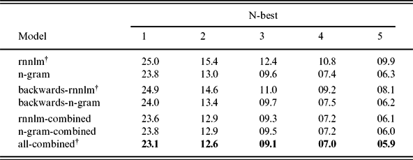
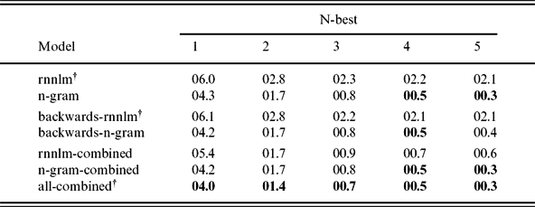
The N-best oracle results (with N = 1 − 5) for the RnnLM experiments for the CMUdict are described in Table 11, and for the Yandex-ru lexicon in Table 12. The tables also illustrate best results from the preceding n-gram smoothing experiments for comparison. Finally, we present model combination and reranking results, as these have proven quite fruitful in this area in recent years (Hahn, Vozila and Bisani Reference Hahn, Vozila and Bisani2012; Schlippe, Quaschningk and Schultz Reference Schlippe, Quaschningk and Schultz2014; Cortesa, Kuznetsov and Mohri Reference Cortes, Kuznetsov and Mohri2014).
Oracle N-best CMUdict WER results for direct decoding with joint RnnLMs.† Averaged over five randomized trials

Oracle N-best Yandex-ru WER results for direct decoding with joint RnnLMs.† Averaged over five randomized trials

For the reranking experiments, a simple formula was used to combine and re-rank N-best results for the various models. First, the the log posteriors for each N-best list, for each system, were normalized to sum to one. Next, a new score was computed for each unique hypothesis by summing the normalized scores across all N models according to the formula hnew = ∑ N n Score(hn ), where Score(hn ) equals the normalized score for hypothesis h and model n, if the hypothesis was predicted by the model, and zero otherwise.
From the results in both tables, it is clear that, while the direct RnnLM results are competitive, they still fall consistently short of the best n-gram only models. The relative superiority of the n-gram models also increases as the size of the N-best increases. There is no statistically significant improvement with regard to the choice of backward and forward models, nevertheless combination of backward and forward models have been shown to be effective in previous works (Schuster and Paliwal Reference Schuster and Paliwal1997), and ensemble methods tend to provide strong and consistent improvements, especially when modeling techniques differ significantly (Schlippe et al. Reference Schlippe, Quaschningk and Schultz2014; Cortesa et al. Reference Cortes, Kuznetsov and Mohri2014). Indeed, all three ensemble reranking results show consistent gains across all N-best orders and both test sets. The all-combined one-best results for the CMUdict also represent a new state-of-the-art on this data set.
The above model combination approach is surprisingly effective, however much more promising techniques are suggested in Cortesa et al. (Reference Cortes, Kuznetsov and Mohri2014), and we expect that these would further improve the above results. In addition, incorporating additional complementary models such as linear-chain conditional random fields (CRFs) (Wu et al. Reference Wu, Allauzen, Hall, Riley and Roark2014) should again further improve the ensemble system. We plan to incorporate these ideas into future work.
The results on the Yandex lexicon indicate the utility of the proposed toolkit to extremely large pronunciation lexica. Nevertheless, another interesting question is whether or not all this training data is in fact necessary. For certain highly regular languages like Spanish or Italian, it is likely that WER/PER improvements plateau with much less data. In order to determine the case for the Yandex dataset, we also investigated the accuracy on the stated test set when utilizing an array of considerably smaller training subsets. In this case, we look only at the performance on the basic forward n-gram models. The results of these experiments are presented in Table 13.
N-best Yandex-ru WER results for forward n-gram models using various subsets of the training corpus. Results are averaged over five randomized trials

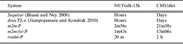
Training times for the smallest (15k entries) and largest (113k entries) training sets (Novak et al. Reference Novak, Minematsu and Hirose2012)

From the table it is clear that, at least in the current case there is ample cause to utilize the full training dataset. While the basic rules are quite simple, the lexicon contains a large number of idiosyncratic entries, acronyms, names and other special words. This may account for the majority of the continued improvement.
7.5 Training and decoding efficiency
The proposed toolkit is both flexible and highly competitive in terms of accuracy, however perhaps its largest advantage is speed. Table 14 from Novak, Minematsu and Hirose (Reference Novak, Minematsu and Hirose2012) compares training times for the proposed toolkit with previously reported results.
The m2m-fst-P for system for the large 113k entry CMUdict training set requires just a tiny fraction of the training time. This turn-around time may be very important for rapid system development. The RNNLM rescoring approach requires more time, however it is still significantly faster than other available options.
7.6 Independent experiments
The proposed toolkit has recently been independently evaluated by several third-party groups in industry and academia. In particular, a series of experiments using large scale pronunciation dictionaries for several different European languages, and comparing a selection of different industry and open-source tools was recently reported in Hahn et al. (Reference Hahn, Vozila and Bisani2012). These experiments were conducted without any input from the authors of this work, however we mention the results here as they represent a completely independent evaluation, which illustrates the flexibility, competitive accuracy and real-world utility of the proposed toolkit and the approach that it embodies.
The experiments in Hahn et al. (Reference Hahn, Vozila and Bisani2012) investigated five different European languages including English, German, French, Italian and Dutch, using large-scale industry pronunciation dictionaries, which all contained over 200k unique words. Six different G2P systems from industry and academia were then evaluated on these dictionaries.
The results of these independent experiments clearly showed that the proposed system is highly competitive with other available industry standard tools. In particular, it consistently outperforms all but seq on each of the large scale datasets, even using the default decoder setup and a relatively simple language model. The performance is also competitive with seq.
Experimental results with the CMU dictionary were also recently successfully replicated in Wu et al. (Reference Wu, Allauzen, Hall, Riley and Roark2014), and the toolkit has been compared and utilized successfully in the ensemble methods described in Schlippe et al. (Reference Schlippe, Quaschningk and Schultz2014).
8 Conclusions
In this work, we have presented the open-source G2P conversion toolkit, Phonetisaurus.
The toolkit provides a variety of standalone, loosely-coupled applications, which can be used to rapidly train sophisticated, high quality G2P conversion models suitable for use in a variety of speech applications.
This work provided detailed discussion on theoretical and practical issues in this area, as well as several novel contributions. A variety of standard language modeling techniques and tools were compared on an equal footing in the context of joint n-gram G2P, using well-known, open-source pronunciation dictionaries.
Detailed discussion of the decoding framework for WFST-based G2P with joint n-gram models was also provided. This also included a decoder suitable for efficient direct decoding of joint sequence RnnLMs.
A suite of experimental results were provided, including the first instance in the literature of using joint sequence RnnLMs for G2P conversion. Ensemble results achieved a new state-of-the-art WER on the well-known CMUdict dataset. In future work in this area, we plan to explore the incorporation of linguistically motivated maximum entropy features as well as the possibility of bi-directional models such as those described in Schuster and Paliwal (Reference Schuster and Paliwal1997).
Independent experimental results as well as preliminary exploratory experimental results for two decoder extensions were also provided. These results illustrated that the proposed toolkit is highly competitive with or superior to the leading solutions in both industry and academia. Experiments illustrating the speed and efficiency of the proposed toolkit were also provided, showing that it dramatically outperforms other solutions in from this perspective.
In the past, many publications have been made describing different joint n-gram models in the context of G2P conversion, however it was difficult to compare these on an even footing due to the lack of a common framework. The loosely-coupled nature of the proposed system, and the ability to directly leverage other mature tools from the Statistical Language Modeling community have made it possible to conduct such evaluations. Furthermore, standard approaches to language model combination, interpolation, class-based models and rescoring are all applicable to the G2P domain, and in many cases may be explored without any direct modification to the proposed toolkit.
The WFST framework also provides a unified ecosystem suitable for incorporating rule-based or language-specific constraints, such as those discussed in Caseiro and Trancoso (Reference Caseiro and Trancoso2002). This is another area ripe for further exploration. Furthermore, the incorporation of additional model types such as linear-chain CRFs (Wu et al. Reference Wu, Allauzen, Hall, Riley and Roark2014), and more advanced ensemble techniques (Schlippe et al. Reference Schlippe, Quaschningk and Schultz2014; Cortesa et al. Reference Cortes, Kuznetsov and Mohri2014) stand to significantly improve the overall quality of the system.
Finally, in recent years other evaluation metrics for G2P have been proposed (Hixon, Schneider and Epstein Reference Hixon, Schneider and Epstein2011), which may correlate better with downstream model usage. Further investigation, implementation and combination of these methods may stand to further improve the validity and utility of results in this area.
The proposed toolkit is released under the BSD license, and is freely available for download (Novak Reference Novak2011). It is our hope that it will continue to enjoy use among speech researchers in industry and academia, and help to further promote innovation in G2P conversion and related areas. Bug reports, fixes and contributions are also welcome.
Acknowledgments
We would like to thank the speech team at Yandex for their help and support in this work.
Appendix A: Tool usage
This section provides several basic usage examples for the main tools provided by the toolkit. Most of the tools contain a wide variety of additional, tunable parameters. The interested reader is referred to the Phonetisaurus toolkit homepage (Novak Reference Novak2011) for more detailed usage instructions and tutorials. The downloads section also includes self-contained experiments suitable for reproducing results from previous publications.