


1. Introduction
The phenomena of particles moving in a density stratified environment is a common occurrence in nature since both the atmosphere and the oceans are, on average, stably stratified. Considering the oceans, for instance, there exist examples of both active (aquatic swimming organisms) and passive (so-called marine snow) particles moving through the stratified pycnocline (Magnaudet & Mercier Reference Magnaudet and Mercier2020), the former often as part of a diurnal migration pattern that has been termed the largest migration on Earth (Martin et al. Reference Martin2020). This work was originally motivated by a rather provocative suggestion (Katija & Dabiri Reference Katija and Dabiri2009; Subramanian Reference Subramanian2010) of the aforementioned migratory pattern leading to an additional biogenic contribution to the mixing of the ocean waters; this is in addition to the two well-known mechanisms of winds and tides (Munk Reference Munk1966). In contrast to the latter two, the energy input in the proposed biogenic contribution occurs at the smallest scales, since the vast majority of the aquatic biomass is concentrated at these scales (the zooplankton or copepods involved in the migration range in size from tens of microns to a few millimetres) (Kunze et al. Reference Kunze, Dower, Beveridge, Dewey and Bartlett2006; Visser Reference Visser2007). As is evident from the arguments put forth in Katija & Dabiri (Reference Katija and Dabiri2009), the validity of the biogenic mixing hypothesis is rooted in the ability of a single small active organism, or a passive particle, to drag along a large amount of fluid during its migration, thereby contributing to the (vertical) mixing of the ocean waters on larger scales. Interestingly, in a homogeneous fluid medium and for any finite Reynolds number, a passive particle can drag an arbitrarily large volume of fluid, over sufficiently long times, on account of the slowly decaying velocity field in its viscous wake (Eames, Gobby & Dalziel Reference Eames, Gobby and Dalziel2003; Chisholm & Khair Reference Chisholm and Khair2017). However, as pointed out by Subramanian (Reference Subramanian2010), the oceans being stably stratified, this dragging motion incurs a potential energy penalty on large enough length scales. The limit of a vanishing stratification (corresponding to a homogeneous fluid medium) is therefore a singular one, in that a small but finite stratification is expected to render the volume dragged by the particle – the so-called drift volume (Darwin Reference Darwin1953; Lighthill Reference Lighthill1956) – finite.
The above description makes it clear that at the heart of the validity of the biogenic mixing hypothesis is the nature of fluid motion induced by an active or passive particle in a stably stratified medium. This study examines the latter problem, that of a small passive particle translating in a stably stratified medium, where ‘small’ refers to the dominance of viscous forces. Consideration of a passive particle is not overly restrictive since even active swimmers, moving along the vertical, attain neutral buoyancy only at a certain instant in time (corresponding to a depth at which the ambient and swimmer densities equal each other). At all other times, such swimmers exert a net force on the ambient. Despite the near field being dominated by the fluid motion induced by the slip velocity on the swimmer surface (Doostmohammadi, Stocker & Ardekani Reference Doostmohammadi, Stocker and Ardekani2012), one expects the net force to invariably play a dominant role in the far field on account of the longer-ranged disturbance velocity field. With this in mind, we consider a passive sphere translating along the direction of stratification at small Reynolds numbers ( $Re$) and viscous Richardson numbers (
 $Ri_v$), the translation assumed to be the result of a density difference. Here,
 $Ri_v ={\gamma a^3 g}/{\mu U}$ measures the relative importance of viscous and buoyancy forces, and is therefore the key dimensionless parameter for motion of small particles in a stratified ambient;
 $\gamma =-{{\rm d}\rho }/{{\rm d}z}$ is the constant density gradient in the ambient(
 $\gamma >0$ for stable stratification, with
 $z$ increasing vertically upwards),
 $a$ the sphere radius,
 $g$ the acceleration due to gravity,
 $\mu$ the fluid viscosity, and
 $U$ the speed of translation. Note that
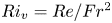 $Ri_v={Re}/{Fr^2}$, where
 $Fr= {U}/{Na}$ is the Froude number that is the usual measure of the importance of stratification in the inviscid limit,
 $N=\sqrt {{g\gamma }/{\rho }}$ here being the Brunt–Väisälä frequency (Turner Reference Turner1979). In a significant departure from most earlier efforts (discussed below), and keeping in mind the oceanic scenario, we consider the Péclet number – defined as
 $Pe = {Ua}/{D}$, where
 $D$ is the diffusivity of the stratifying agent (salt in the oceanic case) – to be large.
As mentioned above, earlier efforts, particularly the ones devoted to analysis of the fluid motion around a moving particle or swimmer, have mostly been restricted to small  $Pe$; an exception is the very recent effort of Shaik & Ardekani (Reference Shaik and Ardekani2020b), and we discuss this in § 4. Motivated by the need to understand laminar jets in a stratified ambient, List (Reference List1971) was the first to characterize the analogue of a Stokeslet (the limiting scenario of a small translating particle, for
 $Re = 0$, approximated as a point force) in a linearly stratified fluid, and for small
 $Pe$. The author considered both vertical and horizontal Stokeslet orientations in two and three dimensions; for the vertical orientation, relevant to the problem analysed here, the motion although fore–aft symmetric was shown to decay away much more rapidly than the
 $O({1}/{r})$ decay characteristic of a Stokeslet in a three-dimensional homogeneous ambient. The resulting weak far-field motion, shown in the paper only for the two-dimensional case, was in the form of toroidal recirculation cells stacked along the direction of stratification. ‘Far field’ here refers to (in units of
 $a$) length scales of
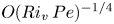 $O(Ri_v\,Pe)^{-{1}/{4}}$, the stratification screening length for
 $Pe \ll 1$; as will be seen below, in Appendix A, the number of such cells is finite. Much later, Ardekani & Stocker (Reference Ardekani and Stocker2010) considered the same problem, but for both passive and active particles modelled as point force and force-dipole singularities, respectively. The density and velocity fields were obtained numerically using a fast Fourier transform technique, the singularities being termed ‘stratlets’. More recently, Fouxon & Leshansky (Reference Fouxon and Leshansky2014) examined the role of turbulence, within the Boussinesq framework, in disrupting the stratification-induced signatures on the flow field around passive particles and active swimmers. As part of their analysis, the authors derived an asymptotic expression for the far-field flow in the absence of turbulence, and that exhibited a rapid algebraic decay, consistent with the findings of the aforementioned studies. Candelier, Mehaddi & Vauquelin (Reference Candelier, Mehaddi and Vauquelin2014) calculated the correction to the Stokes drag on a sedimenting passive particle, for small
 $Pe$, arising from stratification effects in the outer region characterized by scales of
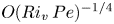 $O(Ri_v\,Pe)^{-{1}/{4}}$; see the discussion in the paragraph after the next one. The authors also determined the history force that characterizes the approach to the terminal settling regime. Wagner, Young & Lauga (Reference Wagner, Young and Lauga2014) examined the mixing efficiencies associated with the flow induced by micro-swimmers, for small
 $Pe$, finding them to be negligibly small.
While the aforementioned efforts have analysed the fluid motion around both passive particles and active swimmers primarily in the small  $Pe$ regime, the motion of a typical particle or small-sized swimmer (zooplankton) in the oceanic ambient, relevant to the biogenic mixing hypothesis, pertains to large
 $Pe$; for instance, a zooplankton of size
 $0.1$ mm moving at speed
 $1$ mm s
 $^{-1}$ in a typical oceanic stratification
 $\gamma =1.67\times 10^{-3}$ kg m
 $^{-4}$ yields
 $Re=0.116$,
 $Ri_v=1.84\times 10^{-8}$ and
 $Pe=100$. Note that the large-
 $Pe$ regime pertains generically to cases where salt is the stratifying agent for particles larger than a few microns, the aforementioned oceanic ambient being only one such instance. The first theoretical effort in this regime is that of Zvirin & Chadwick (Reference Zvirin and Chadwick1975), who calculated the drag enhancement in what we term the Stokes stratification regime below, defined by
 $Re \ll Ri_v^{{1}/{3}} \ll 1$. The calculation was restricted to determining the drag enhancement arising from buoyancy effects in the outer region, on scales of
 $O(Ri_v^{-{1}/{3}})$, corresponding to the stratification screening length – this is the screening length for large
 $Pe$, in contrast to the
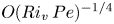 $O(Ri_v\,Pe)^{-{1}/{4}}$ screening length above, for small
 $Pe$, that was obtained by List (Reference List1971) and Ardekani & Stocker (Reference Ardekani and Stocker2010). Similar to the determination by Childress (Reference Childress1964) of the drag correction for the axial motion of a sphere in a rotating fluid, and the calculation by Saffman (Reference Saffman1965) of the inertial lift on a sphere in an ambient simple shear flow, the analysis was done in Fourier space, with the enhancement to the Stokes drag turning out to be
 $O(Ri_v^{{1}/{3}})$, the inverse of the aforementioned screening length. Mehaddi, Candelier & Mehlig (Reference Mehaddi, Candelier and Mehlig2018) have extended the efforts of Candelier et al. (Reference Candelier, Mehaddi and Vauquelin2014) and Zvirin & Chadwick (Reference Zvirin and Chadwick1975) for small and large
 $Pe$, respectively, with
 $Re = 0$, and have obtained the outer-region drag correction for any
 $Pe$, and for small but finite
 $Re$ and
 $Ri_v$. In the process, the authors show that the Zvirin & Chadwick (Reference Zvirin and Chadwick1975) calculation remains valid over an unexpectedly large interval of
 $Pe$, corresponding to
 $Pe \gg Ri_v^{{1}/{3}}$, an aspect that is mirrored in the calculation of the stratification-induced torque for sedimenting anisotropic particles (Varanasi, Marath & Subramanian Reference Varanasi, Marath and Subramanian2022). More recently, Zhang, Mercier & Magnaudet (Reference Zhang, Mercier and Magnaudet2019), by using detailed numerical calculations and an ingenious splitting procedure, showed that the enhancement in drag at low Reynolds numbers comes primarily from the induced baroclinic torque and the resulting change in the flow structure. The enhancement was found to be proportional to
 $Ri_v^{{1}/{3}}$, in agreement with the Zvirin–Chadwick result above, but in opposition to the observations of Yick et al. (Reference Yick, Torres, Peacock and Stocker2009), who obtained a scaling closer to
 $Ri_v^{{1}/{2}}$; the latter mismatch is likely due to additional non-Boussinesq contributions arising from heavily deformed isopycnals close to the sphere.
Very recently, Mercier et al. (Reference Mercier, Wang, Péméja, Ern and Ardekani2020) and Dandekar, Shaik & Ardekani (Reference Dandekar, Shaik and Ardekani2020) have analysed the drag and torque acting on anisotropic disk-shaped particles (and the resulting orientation dynamics) sedimenting in a stratified medium. The experiments reported in Mercier et al. (Reference Mercier, Wang, Péméja, Ern and Ardekani2020) pertain to finite  $Re$ and
 $Ri_v$, and highlight the existence of an edgewise settling regime for sufficiently large
 $Ri_v$ or small
 $Fr$ (in this regard, see also Doostmohammadi & Ardekani Reference Doostmohammadi and Ardekani2014; Mrokowska Reference Mrokowska2018, Reference Mrokowska2020a,Reference Mrokowskab); this is in contrast to the broadside-on settling regime known for small to moderate
 $Re$ in a homogeneous ambient (Cox Reference Cox1965; Dabade, Marath & Subramanian Reference Dabade, Marath and Subramanian2015; Anand, Ray & Subramanian Reference Anand, Ray and Subramanian2020). The theoretical effort of Dandekar et al. (Reference Dandekar, Shaik and Ardekani2020) evaluates the hydrodynamic force and torque on an arbitrarily shaped body in a linearly stratified ambient for arbitrary
 $Pe$, and finds a torque, arising from the ambient stratification, for chiral particles. The role of stratification in the orientation dynamics of achiral particles, such as the ones used in Mercier et al. (Reference Mercier, Wang, Péméja, Ern and Ardekani2020), has been analysed in detail in Varanasi et al. (Reference Varanasi, Marath and Subramanian2022). In the present context, we only note that although the aforementioned studies, for both spherical and non-spherical particles, pertain to the large-
 $Pe$ limit, the fluid motion induced by the translating particle was not examined in detail.
The primary motivation for our calculation is to determine eventually the drift volume associated with a particle translating in a stably stratified ambient, and thereby estimate the importance of the biogenic mixing contribution. Now, as mentioned above, the infinite-time drift volume is divergent, for any finite  $Re$, in a homogeneous ambient (Eames et al. Reference Eames, Gobby and Dalziel2003; Chisholm & Khair Reference Chisholm and Khair2017; Subramanian Reference Subramanian2010), this divergence arising from the slow
 $O({1}/{r})$ decay of velocity field within the far-field wake,
 $r$ being the distance downstream from the translating particle. For
 $Re = 0$, the velocity field decays as
 $O({1}/{r})$, at distances large compared to the particle size, regardless of the direction, and as a result, the drift volume diverges for any finite time. This implies that the finiteness of the drift volume, for a weakly stratified ambient pertaining to the aforementioned Stokes stratification regime, must arise from the transition of the far-field fluid motion from an
 $O({1}/{r})$ Stokesian decay to a more rapid decay beyond the
 $O(Ri_v^{-{1}/{3}})$ stratification screening length. Thus for small
 $Re$, unlike the drag problem considered in Zvirin & Chadwick (Reference Zvirin and Chadwick1975), one expects the dominant contribution to the drift volume to arise from the fluid motion far from the sphere, or in other words, the outer region. It is with this in mind that the analysis here is restricted to the linearized equations in the far field. One may nevertheless question the relevance of this linearization, given that the motion in the outer region is influenced indirectly by the heavily deformed isopycnals, close to the sphere, for large
 $Pe$. However, these deformed isopycnals contribute to a localized buoyant envelope around the sphere, and at large distances, one may regard the combination of the envelope and the sphere as an effective point force, albeit of a different magnitude, as far as the outer region is concerned; the linearity of the outer-region equations implies that the nature of fluid motion is independent of the magnitude of the force. More detailed scaling arguments pertaining to the velocity and density fields in the inner region (length scales of
 ${O}(a)$) are given in § 4.
The remainder of the paper is organized as follows. In the next section, we present the quasi-steady governing equations for the fluid motion under the Boussinesq approximation, and a scaling analysis to determine the screening lengths arising from the effects of inertia and stratification, the latter in the limit of large  $Pe$. The linearized equations in the outer region are then solved using a Fourier transform approach (Childress Reference Childress1964; Saffman Reference Saffman1965). The velocity and density fields are written as Fourier integrals in the aforementioned large-
 $Pe$ limit, and in the so-called Stokes stratification regime (defined by
 $Re \ll Ri_v^{1/3}$) when buoyancy forces are dominant over inertial ones. In § 3, we first obtain the streamline patterns and isopycnals from a numerical evaluation of the Fourier integrals. Later, in § 3.3, the results are compared to analytical approximations valid for distances much greater than the
 $O(Ri_v^{-{1}/{3}})$ screening length; the results obtained are also contrasted with analogous results, obtained in the small-
 $Pe$ limit, in Appendix A. Regardless of
 $Pe$, the role of stratification, at distances of order the stratification screening length, is to suppress vertical motion. For small
 $Pe$, this suppression is complete, while for large
 $Pe$, vertical motion remains confined to the region near the rear stagnation streamline in the form of a reverse jet. The near-horizontal motion, at distances greater than the screening length above, is restricted to a far-field ‘horizontal’ wake surrounding the translating particle. As shown (for large
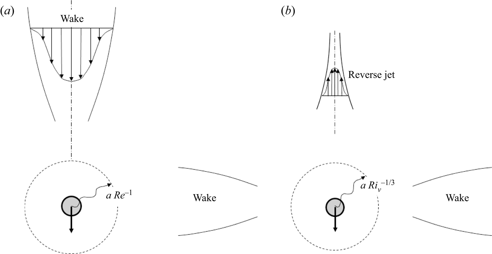
 $Pe$) in figure 1, via a simple schematic, such a wake is in contrast to the familiar vertical wake that arises behind the particle in a homogeneous ambient. The various scalings pertaining to the flow structure in figure 1(b) are developed in more detail in § 3.4. In the concluding § 4, we summarize our work, and follow this up with scaling arguments pertaining to the inner region dynamics and drift volume.
Schematic comparing the far-field flow structure induced by the slow translation of a sphere in (a) a homogeneous ambient for  $Re \ll 1$ (with a vertical viscous trailing wake), and (b) a stratified ambient for
 $Re,Ri_v \ll 1$,
 $Pe \gg 1$ (with a horizontal axisymmetric wake and a reverse jet).

2. The disturbance fields in a stable linearly stratified ambient
Considering a sphere moving vertically in an unbounded stably stratified fluid with a linear stratification profile  ${{\rm d}\rho }/{{\rm d}z}=-\gamma$ (
 $\gamma > 0$),
 $z$ being the vertical coordinate, and using
 $a$,
 $U$ and
 $\gamma a$ for the length, velocity and density scales, respectively, the non-dimensional continuity equation, the Navier–Stokes equations and the convection–diffusion equation, in a sphere-fixed reference frame, are as follows:
 \begin{gather} \boldsymbol{\nabla} \boldsymbol{\cdot} \boldsymbol{u}=0, \end{gather}
 \begin{gather}Re\,[\boldsymbol{u} \boldsymbol{\cdot} \boldsymbol{\nabla} \boldsymbol{u}]={-}\boldsymbol{\nabla} p+\nabla^2 \boldsymbol{u} - Ri_v\,\rho_f \boldsymbol{1_z}, \end{gather}
 \begin{gather}1-w+\boldsymbol{u} \boldsymbol{\cdot} \boldsymbol{\nabla} \rho_f= \frac{1}{Pe}\,\nabla^2 \rho_f, \end{gather}
with the boundary conditions
 \begin{gather} \boldsymbol{u}=0, \quad \boldsymbol{n} \boldsymbol{\cdot} \boldsymbol{\nabla}{\rho_f} ={-}\boldsymbol{n} \boldsymbol{\cdot} \boldsymbol{1}_{\boldsymbol{z}} \quad \text{at} \ r=1, \end{gather}
 \begin{gather}\boldsymbol{u} \rightarrow \boldsymbol{1}_{\boldsymbol{z}}, \quad \rho_f \rightarrow 0 \quad \text{as} \ r \rightarrow \infty, \end{gather}
where  $r (=|\boldsymbol {x}|)$ is the non-dimensional distance from the sphere, and
 $w$ in (2.3) is the vertical velocity component (Candelier et al. Reference Candelier, Mehaddi and Vauquelin2014; Mehaddi et al. Reference Mehaddi, Candelier and Mehlig2018; Shaik & Ardekani Reference Shaik and Ardekani2020a). The total density in the aforementioned reference frame is given by
 $\rho (z)=\rho _0+t-z+\rho _f$, and the term involving
 $1-w$ in (2.3) denotes the convection of the base-state stratification (along the vertical) by the perturbation velocity field. Note that the Boussinesq approximation has been used above to neglect the density disturbance in the convective terms of the equations of motion, so
 $Re$ in (2.2) is based on an appropriate reference density. Further, in taking
 $\rho _f$ in particular to be independent of time, we have assumed a quasi-steady state to be achieved for long times. This assumption is examined in § 4 for both the inner (
 $r \sim O(1)$) and outer (
 $r \geq O(Ri_v^{-{1}/{3}})$) regions.
As is well known, although we examine the limit  $Re, Ri_v \ll 1$, the inertial and stratification terms in (2.2) cannot be neglected. The Stokes equations are not a uniformly valid approximation, and the aforementioned terms become comparable to the leading-order viscous terms at distances large compared to the particle size. As discussed in the Introduction, for a weakly stratified ambient, such length scales are expected to determine the drift volume, the large magnitude of which underlies the biogenic mixing hypothesis. For a homogeneous fluid, the length scale (in units of
 $a$) at which inertial forces first become comparable to viscous forces is
 $Re^{-1}$, referred to here as the inertial screening length. Obtaining a similar estimate for the buoyancy forces requires one to obtain the far-field behaviour of the density field, which in turn depends on whether
 $Pe$ is large or small.
For  $Pe \rightarrow \infty$, one neglects the diffusion term in (2.3) to obtain
 $\boldsymbol {u} \boldsymbol {\cdot } \boldsymbol {\nabla }\rho _f \sim (1-w)$. Using
 $(1-w) \sim O({1}/{r})$ for the Stokeslet field, one has
 $\rho _f \sim O(1)$, so the buoyancy forcing term in (2.2) is
 $O(Ri_v)$. Equating this to the decaying viscous forces of
 $O(1/r^3)$, one obtains the large-
 $Pe$ stratification screening length
 $l_c \sim Ri_v^{-{1}/{3}}$, as shown originally by Zvirin & Chadwick (Reference Zvirin and Chadwick1975). Keeping in mind the Stokesian rates of decay for
 $r \gg 1$, the disturbance fields on length scales of order the aforementioned screening length, which define the outer region, may be expanded as
 $\boldsymbol {u}=\boldsymbol {1}_{\boldsymbol {z}}+Ri_v^{{1}/{3}}\,\tilde {\boldsymbol {u}}(\tilde {\boldsymbol {r}})$,
 $p=p_{\infty }+Ri_v^{{2}/{3}}\,\tilde {p}(\tilde {\boldsymbol {r}})$ and
 $\rho _f=\tilde {\rho }_f(\tilde {\boldsymbol {r}})$, where here,
 $\tilde {\boldsymbol {r}} = Ri_v^{{1}/{3}}\,{\boldsymbol r}$ is the scaled outer-region coordinate. One obtains the following outer-region equations:
 \begin{gather} \tilde{\boldsymbol{\nabla}}\boldsymbol{\cdot} \tilde{\boldsymbol{u}}=0, \end{gather}
 \begin{gather}\alpha_\infty\,\frac{\partial \tilde{\boldsymbol{u}}}{\partial \tilde z}={-}\tilde{\boldsymbol{\nabla}} \tilde p +\tilde \nabla^2 \tilde{\boldsymbol{u}}-[\tilde{\rho}_f+6{\rm \pi}\,\delta(\boldsymbol{ \tilde r})]\,\boldsymbol{1}_{\boldsymbol{z}}, \end{gather}
 \begin{gather}-\boldsymbol{1}_{\boldsymbol{z}}\boldsymbol{\cdot}\tilde u+ \frac{\partial\tilde{\rho}_f}{\partial \tilde z} = \beta_\infty\,\tilde \nabla^2 \tilde{\rho}_f. \end{gather}
Here,  $\alpha _\infty$ and
 $\beta _\infty ^{-1}$ are given by
 ${Re}/{Ri_v^{1/3}}$ and
 ${Pe}/{Ri_v^{1/3}}$, respectively, and denote the ratios of the large-
 $Pe$ stratification screening length to the inertial (
 $Re^{-1}$) and convective (
 $Pe^{-1}$) screening lengths. Note that the boundary condition on the particle surface has now been replaced by a point force on the right-hand side of (2.7). In the Stokes stratification regime, corresponding to
 $Re \ll Ri_v^{{1}/{3}}$, one can set
 $\alpha _\infty$ in (2.7) to zero. Although our primary focus is on the limit
 $\beta _\infty \rightarrow 0$ (
 $Pe\rightarrow \infty$), retaining a small but finite
 $\beta _\infty$ is important. While the structure of the disturbance fields almost everywhere in the domain is independent of
 $\beta _\infty$ in this limit, in § 3.2 it is shown that a small but finite
 $\beta _\infty$ crucially affects the structure of the fields right behind the translating sphere. Further, a non-zero
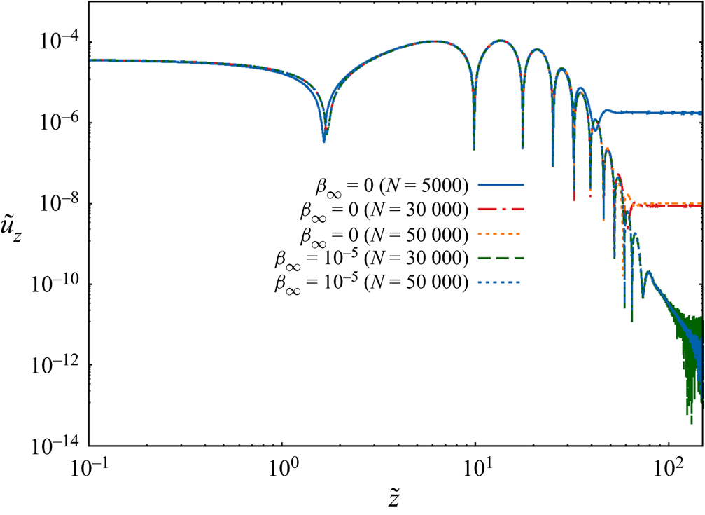
 $\beta _\infty$ is also important for obtaining numerically converged results for the Fourier integrals (see Appendix C).
Defining the relations between the physical space and Fourier transformed disturbance fields as
 \begin{gather} \hat{f}(\boldsymbol{k})= \int f(\boldsymbol{x}) \,{\rm e}^{-{\rm i}\boldsymbol{k}\boldsymbol{\cdot}\boldsymbol{r}} \,{\rm d}\kern0.06em \boldsymbol{x}, \end{gather}
 \begin{gather}f(\boldsymbol{x})= \frac{1}{(2{\rm \pi})^3}\int \hat{f}(\boldsymbol{k})\, {\rm e}^{{\rm i}\boldsymbol{k}\boldsymbol{\cdot}\boldsymbol{r}} \,{\rm d}\boldsymbol{k}, \end{gather}
with  $f(\boldsymbol {x})$ denoting the relevant disturbance field, and Fourier transforming (2.6)–(2.8), one obtains, after some algebra, the velocity and density disturbance fields as the integrals
 \begin{gather} \tilde{\boldsymbol{u}} (\boldsymbol{\tilde{r}}) = \frac{-3}{4{\rm \pi}^2} \int \frac{({\rm i}k_3+\beta_\infty k^2)k^2 (\boldsymbol{1}_{\boldsymbol{z}}-k_3\boldsymbol{k}/k^2)}{({\rm i}k_3+\beta_\infty k^2)k^4+k_t^2} \,{\rm e}^{{\rm i}\boldsymbol{k}\boldsymbol{\cdot}\tilde{\boldsymbol{r}}} \,{\rm d}\boldsymbol{k}, \end{gather}
 \begin{gather}\tilde{\rho}_f(\tilde{\boldsymbol{r}}) = \frac{-3}{4{\rm \pi}^2} \int \frac{k_t^2}{({\rm i}k_3+\beta_\infty k^2)k^4+k_t^2} \,{\rm e}^{{\rm i}\boldsymbol{k}\boldsymbol{\cdot} \tilde{\boldsymbol{r}}} \,{\rm d}\boldsymbol{k}. \end{gather}
Here,  $k_t = (k^2-{k_3}^2)^{{1}/{2}}$ is the magnitude of the wavevector projected onto the plane perpendicular to the translation direction.
3. Results and discussion
Herein, we analyse the axial velocity and density disturbance fields, and the associated streamline and isopycnal patterns, in the convection-dominant limit, by using a combination of numerics (Gauss–Legendre quadrature integration) and far-field asymptotics. As already mentioned in the Introduction, the results are for the case of buoyancy forces being dominant (the Stokes stratification regime), corresponding to  $\alpha _\infty \ll 1$. Analogous results for the diffusion dominant limit are obtained in Appendix A, and are used below for comparison purposes. The role of weak inertial effects, and the resulting large-scale structure of the flow field, in both the diffusion and convection-dominant limits, is discussed via scaling arguments towards the end of this section.
The Fourier integrals given by (2.11) and (2.12) are expressed in a spherical coordinate system with its polar axis aligned with the translation direction. The integral over the azimuthal angle ( $\phi$) can then be carried out analytically, and the resulting expressions for the axial velocity and density disturbance are given by
 \begin{gather} \tilde{u}_{z}={-}\frac{3}{2{\rm \pi}}\int_0^\infty {\rm d}k \int_0^{\rm \pi} {\rm d}\theta\, \frac{\sin^3\theta\,({\rm i}k^3\cos\theta+\beta_{\infty}k^4)\,J_0(k\tilde{r}_t\sin \theta)\,{\rm e}^{{\rm i}k\tilde{z}\cos\theta}}{{\rm i}k^3\cos\theta+\beta_{\infty}k^4+\sin^2\theta}, \end{gather}
 \begin{gather}\tilde{\rho}_f=\frac{-3}{2{\rm \pi}}\int_0^\infty {\rm d}k \int_0^{\rm \pi} {\rm d}\theta\,\frac{k^2\sin^3\theta\, J_0(k\tilde{r}_t\sin \theta)\,{\rm e}^{{\rm i}k\tilde{z}\cos\theta}}{{\rm i}k^3\cos\theta+\beta_{\infty}k^4+\sin^2\theta}, \end{gather}
where  $J_0(x)$ is the zeroth-order Bessel function of the first kind. Note that since the problem is axisymmetric, the fields are written as functions of (
 $\tilde r_t,\tilde z$), with
 $\tilde r_t$ and
 $\tilde z$ being the distances along and orthogonal to the direction of translation. Not including the complex exponential, the Fourier integrand for the density disturbance field in (3.2), for large
 $k$, decays as
 ${1}/{k^{5/2}}$ for
 $\beta _\infty \neq 0$, and as
 ${1}/{k^{3/2}}$ for
 $\beta _\infty = 0$; that for the axial velocity in (3.1) decays only as
 ${1}/{k^{1/2}}$ regardless of
 $\beta _\infty$, this slow decay reflecting the
 ${1}/{r}$ decay of the Stokeslet for small
 $r$. As a result, an accurate evaluation of (3.1) relies essentially on cancellation induced by the complex Fourier exponential. To facilitate numerical evaluation, we therefore separate out the Stokeslet contribution, writing the axial velocity integral above as
 \begin{equation} \tilde{u}_{z}=\frac{-3(2+\tilde{r}_t^2/\tilde{z}^2)}{4\,|\tilde{z}|\,(1+\tilde{r}_t^2/\tilde{z}^2)^{{3}/{2}}} +\frac{3}{2{\rm \pi}}\int_0^\infty {\rm d}k \int_0^{\rm \pi} {\rm d}\theta\,\frac{\sin^5\theta\,J_0(k\tilde{r}_t\sin \theta)\,{\rm e}^{{\rm i}k\tilde{z}\cos\theta}}{{\rm i}k^3\cos\theta+\beta_{\infty}k^4+\sin^2\theta}, \end{equation}
where the integrand in (3.3) now decays as  ${1}/{k^{9/2}}$, for sufficiently large
 $k$, for any finite
 $\beta _\infty$. The Stokes streamfunction may be found using the relation
 $\bar {u}_z=({1}/{\tilde {r}_t})({\partial \tilde {\psi }_s}/{\partial \tilde {r}_t})$ and is given by
 \begin{equation} \tilde{\psi}_s=\frac{-3\tilde{r}_t^2}{4(\tilde{r}_t^2+\tilde{z}^2)^{{1}/{2}}} +\frac{3\tilde{r}_t}{2{\rm \pi}}\int_0^\infty {\rm d}k \int_0^{\rm \pi} {\rm d}\theta\,\frac{\sin^4\theta\,J_1(k\tilde{r}_t\sin \theta)\,{\rm e}^{{\rm i}k\tilde{z}\cos\theta}}{k({\rm i}k^3\cos\theta+\beta_{\infty}k^4+\sin^2\theta)}. \end{equation}
Note from (3.2) and (3.3) that although our interest is in the limit  $\beta _\infty = 0$, corresponding to convection effects being infinitely dominant, we have retained the terms proportional to
 $\beta _\infty$ in the integrands. One reason is ease of numerical evaluation (see Appendix C). The second reason is the sensitive dependence of the structure of both the velocity and density fields, in the neighbourhood of the rear stagnation streamline, on
 $\beta _\infty$; the density field in particular diverges for
 $\beta _\infty = 0$ (see Appendix D).
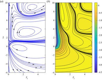
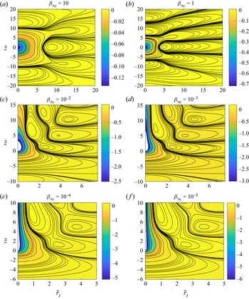
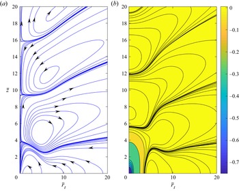
Figure 2 shows the streamline pattern and the isopycnal contours for the smallest  $\beta _\infty (=10^{-5})$ accessed in our calculations. The numerical evaluation of the above integrals, leading to these patterns, is carried out using Gauss–Legendre quadrature after first using
 $k=\tan \hat {k}_f$ to transform the original
 $k$ interval to a finite one in
 $\hat {k}_f$. The limited spatial extent of the domain in figure 2 is on account of the numerical difficulties involved in calculating the far-field isopycnals; the streamline pattern alone, over a larger spatial domain, appears later, in figure 8(f). Nevertheless, the fore–aft asymmetry of both the streamline and isopycnals patterns is evident readily from figure 2, and is in contrast to those in the diffusion-dominant limit (figure 12 in Appendix A). Buoyancy forces are seen to transform the essentially vertical motion close to the origin, to primarily horizontal motion at larger radial distances, with this horizontal motion occurring within multiple recirculating cells stacked along the vertical. Interestingly and perhaps surprisingly (if one's intuition is based on the cellular disturbance, flow fields set up internal gravity waves in an unbounded stratified ambient), the far-field analysis in the next subsection shows the number of such cells to be finite, likely on account of the neglect of inertial effects.
(a) Streamlines and (b) isopycnals, for a translating sphere in a linearly stratified fluid, in the convection-dominant limit ( $\beta _\infty = 10^{-5}$), in the Stokes stratification regime (
 $Re \ll Ri_v^{{1}/{3}}$). In the point-particle approximation used, the sphere is at the origin and moving vertically downwards.

The streamline pattern in figure 2(a) is, in fact, quite analogous to figure 2(d) in Zhang et al. (Reference Zhang, Mercier and Magnaudet2019), which, although it pertains to the region around a finite sphere of order its own size, corresponds to a relationship between  $Re$ and
 $Ri_v$ consistent with the Stokes stratification regime. The fore–aft asymmetry seen in figure 2 may be anticipated from the integral expressions in (3.1)–(3.4), where, unlike the
 $Pe = 0$ (
 $\beta _\infty = \infty$) limit, one can no longer replace the complex exponential by a cosine (see (A8) in Appendix A). Apart from the different shapes and numbers of the recirculating cells in front of and behind the translating sphere, there is also the appearance of a radially localized but vertically extended structure, in the streamline pattern, in the rear. As will be seen below, this corresponds to a buoyant reverse jet that develops behind the particle with decreasing
 $\beta _\infty$ (see figures 8a–f). The far-field analysis in the subsections below points to both a stratification-induced wake in the convection-dominant limit with a structure that is insensitive to
 $\beta _\infty$ (for
 $\beta _\infty \ll 1$), and the buoyant reverse jet mentioned above whose structural features depend essentially on
 $\beta _\infty$.
3.1. Far-field wake analysis
At radial distances much greater than the stratification screening length, one expects largely horizontal motion. As a consequence, the characteristic length scale in the vertical direction will be much smaller than that along the horizontal. The Fourier integrals in (2.11) and (2.12), for length scales large compared to  $Ri_v^{-{1}/{3}}$, may therefore be simplified using
 $k_3 \gg k_t$, leading to
 \begin{gather} \tilde{u}_z (\tilde{\boldsymbol{r}}) = \frac{-3}{4{\rm \pi}^2} \int \frac{{\rm i}k_3k_t^2}{{\rm i}k_3^5+k_t^2} \,{\rm e}^{{\rm i}\boldsymbol{k}\boldsymbol{\cdot}\tilde{\boldsymbol{r}}} \,{\rm d}\boldsymbol{k}, \end{gather}
 \begin{gather}{\tilde{\rho}_f}(\tilde{\boldsymbol{r}}) = \frac{-3}{4{\rm \pi}^2} \int \frac{k_t^2}{{\rm i}k_3^5+k_t^2} \,{\rm e}^{{\rm i}\boldsymbol{k}\boldsymbol{\cdot}\tilde{\boldsymbol{r}}} \,{\rm d}\boldsymbol{k}, \end{gather}
where we have set  $\beta _\infty = 0$. The integrals in (3.5) and (3.6), which govern the structure of the stratification-induced wake at large radial distances, may be reduced to the following one-dimensional integrals, written in terms of the similarity variable
 $\tilde {\eta } = {\tilde z}/{\tilde {r}_t^{{2}/{5}}}$, via contour integration (see Appendix B for details):
 \begin{align} \tilde{u}_{z}&=\begin{cases} {-\dfrac{15{\rm i}}{2\tilde{r}_t^{14/5}}}\displaystyle\int_0^\infty m^6\,J_0[m^{5/2}][Q_1q_1\,{\rm e}^{{\rm i}q_1m\tilde{\eta}}+Q_2q_2\,{\rm e}^{{\rm i}q_2m\tilde{\eta}}+Q_3q_3\,{\rm e}^{{\rm i}q_3m\tilde{\eta}}]\,{\rm d}m & (\tilde \eta>0),\\ \dfrac{15{\rm i}}{2\tilde{r}_t^{14/5}}\displaystyle\int_0^\infty m^6\,J_0[m^{5/2}][Q_4q_4\,{\rm e}^{{\rm i}q_4m\tilde{\eta}}+Q_5q_5\,{\rm e}^{{\rm i}q_5m\tilde{\eta}}]\,{\rm d}m & (\tilde \eta<0),\end{cases} \end{align}
 \begin{align} \tilde{\rho}_f &=\begin{cases} {-\dfrac{15}{2\bar{r}_t^{12/5}}}\displaystyle\int_0^\infty m^5\,J_0[m^{5/2}][Q_1\,{\rm e}^{{\rm i}q_1m\tilde{\eta}}+Q_2\,{\rm e}^{{\rm i}q_2m\tilde{\eta}}+Q_3\,{\rm e}^{{\rm i}q_3m\tilde{\eta}}]\,{\rm d}m & (\tilde \eta>0), \\ \dfrac{15}{2\tilde{r}_t^{12/5}}\displaystyle\int_0^\infty m^5\,J_0[m^{5/2}][Q_4\,{\rm e}^{{\rm i}q_4m\tilde{\eta}}+Q_5\,{\rm e}^{{\rm i}q_5m\tilde{\eta}}]\,{\rm d}m & (\tilde \eta<0),\end{cases} \end{align}
 \begin{align} \tilde u_{r_t}&=\begin{cases} {-\dfrac{15}{2\tilde{r}_t^{11/5}}}\displaystyle\int_0^\infty m^{9/2}\,J_1[m^{5/2}][Q_1q_1^2\,{\rm e}^{{\rm i}q_1m\tilde{\eta}}+Q_2q_2^2\,{\rm e}^{{\rm i}q_2m\tilde{\eta}}+Q_3q_3^2\,{\rm e}^{{\rm i}q_3m\tilde{\eta}}]\,{\rm d}m & (\tilde \eta>0),\\ \dfrac{15}{2 \tilde{r}_t^{11/5}}\displaystyle\int_0^\infty m^{9/2}\,J_1[m^{5/2}][Q_4q_4^2\,{\rm e}^{{\rm i}q_4m\tilde{\eta}}+Q_5q_5^2\,{\rm e}^{{\rm i}q_5m\tilde{\eta}}]\,{\rm d}m & (\tilde \eta<0).\end{cases} \end{align}
Here, the  $Q_n$ and
 $q_n$ (
 $n=1,2,3,4,5$) are complex-valued constants given in Appendix B. The fore–aft asymmetry implies that one has different asymptotic approximations depending on the sign of
 $\tilde {\eta }$ (or
 $\tilde {z}$). Nevertheless, the above self-similar forms point to a far-field wake that includes the horizontal plane containing the settling sphere, and whose vertical extent grows as
 $z \propto Ri_v^{-{1}/{5}}\,{r}_t^{{2}/{5}}$, with
 $z$ and
 $r_t$ being measured in units of
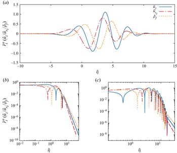
 $a$. The axial and radial velocity profiles, and the density disturbance profiles, obtained from a numerical evaluation of the one-dimensional integrals above, are shown on both linear and logarithmic scales in figure 3, with the logarithmic plot clearly highlighting the zero-crossings at larger distances. The logarithmic plot also shows that while there are a finite number of zero-crossings, implying a finite number of recirculating cells (similar to
 $Pe = 0$; see figure 13 in Appendix A), they differ in number for negative and positive
 $\tilde {\eta }$, with fewer zero-crossings for negative
 $\tilde {\eta }$. This implies fewer recirculating cells below the settling sphere, and is consistent with the streamline pattern in figure 2 (see also figure 8f below). One may also obtain the large-
 $\tilde {\eta }$ asymptotic forms from (3.7)–(3.9), which govern the eventual algebraic decay of the disturbance fields beyond the final zero-crossing; these are given by
 $\lim _{|\tilde {\eta }| \rightarrow \infty } [\tilde {u}_z^+,\tilde {u}_z^-] \equiv [{3240}/{(r_t^{{14}/{5}}\tilde {\eta }^7)},-{2160}/{(r_t^{{14}/{5}}\tilde {\eta }^7)}]$,
 $\lim _{|\tilde {\eta }| \rightarrow \infty } [\tilde {u}_{r_t}^+,\tilde {u}_{r_t}^-] \equiv [{11\,340}/{(r_t^{{11}/{5}}\tilde {\eta }^8)},-{7560}/{(r_t^{{11}/{5}}\tilde {\eta }^8)}]$ and
 $\lim _{|\tilde {\eta }| \rightarrow \infty } [\tilde {\rho }_f^+,\tilde {\rho }_f^-] \equiv [-{540}/{(r_t^{{12}/{5}}\tilde {\eta }^6)}, {360}/{(r_t^{{12}/{5}}\tilde {\eta }^6)}]$, where the ‘
 $+$’ and ‘
 $-$’ superscripts correspond to positive and negative
 $\tilde {\eta }$, respectively. These asymptotes, and the above approximate profiles based on the one-dimensional integrals above, will be compared to the exact (numerical) fields in § 3.3. Analogous asymptotes pertaining to the diffusion-dominant limit are derived in Appendix A, the difference being the definition of the similarity variables (
 $\bar {\eta } \propto r/z^{{1}/{3}}$, which reflects the growth of the small-
 $Pe$ wake) and the identity of the positive and negative
 $\bar {\eta }$ asymptotes due to fore–aft symmetry.
The axial velocity, radial velocity and density disturbance profiles, within the far-field wake region, in the convection-dominant limit ( $Pe \gg 1$) pertaining to the Stokes stratification regime: (a) the disturbance fields on a linear scale. The absolute value of the disturbance fields on a logarithmic scale is shown for (b) negative
 $\tilde \eta$, and (c) positive
 $\tilde \eta$. Here,
 $n = 14/5$,
 $11/5$ and
 $12/5$ for
 $u_z$,
 $u_{r_t}$ and
 $\rho _f$, respectively. The aforementioned wake includes the plane of the settling sphere, and grows in vertical extent as
 $z \propto Ri_v^{{2}/{15}}\,{r}_t^{{2}/{5}}$.

The structure of the far-field wake may also be characterized in terms of the  $\tilde {\eta }$-moments of the disturbance fields above. The motion being largely horizontal, it is the moments of the radial velocity field that are the most important. A calculation using the far-field approximation above (see (3.9)) shows that the zeroth and first moments of the radial velocity field in the wake vanish, and that the second moment, given by
 $\int _{-\infty }^\infty \tilde {\eta }^2 \tilde {u}_{r_t} \,{\rm d}\tilde {\eta } = 6$, is the first non-trivial member of the moment hierarchy. (Interestingly, this may also be seen from direct neglect of the viscous term
 $ik_3k^4$ in the original Fourier integral (2.11), and additionally setting
 $\beta _\infty = 0$; the radial velocity may now be obtained in terms of generalized functions as
 $\tilde u_{r_t} = ({3}/{\tilde {r}_t})\delta ''(z)$, which yields the same value for the second moment.) The moment-based characterization above offers an interesting contrast to the known solution for the motion induced by a sphere settling through a linearly stratified ambient in the linearized inviscid approximation, when stratification forces are (infinitely) dominant. As shown in Vladimirov & Li'in (Reference Vladimirov and Li'in1991), the motion is strictly horizontal and restricted to an infinite horizontal slab whose upper and lower planes bound the sphere. Within this slab, the fluid moves radially inwards (outwards) in the rear (front) half of the translating sphere. The nature of this motion is understood easily from the changing size of the sphere cross-section in a given horizontal plane, and the requirement of satisfying the impenetrability condition at the sphere surface. In two dimensions (that is, a settling circular cylinder), the horizontal velocity field is a constant, while in three dimensions (a settling sphere), the radial motion in a transverse plane would have a
 $1/r_t$ dependence consistent with incompressibility. Such a motion has a dipolar character with a non-trivial first moment for the radial velocity. In contrast, as already seen, the structure of the far-field wake above does not exhibit the aforementioned structure. This is because although the Stokeslet in the inner region has a radial component consistent with the symmetry of the linearized inviscid solution above (directed inwards behind the sphere and outwards in front of it), the Stokeslet is screened by the buoyancy forces induced in a surrounding volume with a linear dimension of
 $O(Ri_v^{-{1}/{3}})$. As a result, the wake velocity field on length scales much larger than
 $O(Ri_v^{-{1}/{3}})$ has the symmetry pertaining to a force-dipole consisting of the original Stokeslet and an effective upward force arising from the volumetric distribution of induced buoyancy forces.
3.2 Far-field jet analysis
The large- $\tilde {\eta }$ asymptotes for the axial velocity and density disturbance fields in the convection-dominant limit, given in the previous subsection, are seen to be independent of
 $\tilde {r}_t$, with the radial disturbance field being
 $O(\tilde {r}_t)$ for
 $\tilde {z} \rightarrow 0$. Thus one expects these asymptotes to remain valid along the stagnation streamline (
 $\tilde {r} = 0$) at distances large compared to
 $Ri_v^{-{1}/{3}}$ (that is, for large
 $\tilde {z}$). While this is true for the diffusion-dominant limit, it is valid only for the front stagnation streamline for
 $Pe \gg 1$; thus
 $\tilde {u}_z = -{2160}/{\tilde {z}^7}$ and
 $\rho _f = {360}/{\tilde {z}^6}$ for large negative
 $\tilde {z}$. However, the wake approximation in the subsection above, and therefore the large-
 $\tilde {\eta }$ approximations derived from it, are no longer valid in the vicinity of the rear stagnation streamline. The pronounced asymmetry in the streamline pattern in figure 2, and the predominantly vertical motion behind the sphere, are already indicative of the breakdown of this approximation. The neighbourhood of the rear stagnation streamline, at large distances, corresponds to large positive
 $\tilde {z}$ and small
 $\tilde {r}_t$. In Fourier space, this is equivalent to
 $k_3 \ll k_t$, the opposite of the wake approximation above, and the Fourier integrals now take the form
 \begin{gather} \tilde{\boldsymbol{u}} (\tilde{\boldsymbol{r}}) ={-}\frac{3 {\rm i}}{4{\rm \pi}^2}\int \frac{k_3k_t^2 (\boldsymbol{1}_{\boldsymbol{z}}-k_3\boldsymbol{k}/k^2)}{{\rm i}k_3k_t^4+k_t^2+\beta_\infty k_t^6} \,{\rm e}^{{\rm i}\boldsymbol{k}\boldsymbol{\cdot}\tilde{\boldsymbol{r}}}\,{\rm d}\boldsymbol{k}, \end{gather}
 \begin{gather}{\tilde{\rho}_f} (\tilde{\boldsymbol{r}}) ={-}\frac{3}{4{\rm \pi}^2}\int \frac{k_t^2}{{\rm i}k_3k_t^4+k_t^2+\beta_\infty k_t^6}\,{\rm e}^{{\rm i}\boldsymbol{k}\boldsymbol{\cdot}\tilde{\boldsymbol{r}}}\,{\rm d}\boldsymbol{k}. \end{gather}
Unlike the wake approximation above, we retain the  $O(\beta _\infty )$ terms in the integrands, in anticipation of the fact that the reverse jet that we find below has a structure that depends crucially on
 $\beta _\infty$ even in the limit
 $\beta _\infty \ll 1$. The integrals in (3.10) and (3.11) can be simplified further by contour integration in the complex-
 $k_3$ plane. From the denominator of the integrand in (3.10) and (3.11), one notes that the only pole exists in the upper half of the complex plane, being given by
 $k_3={\rm i}({(\beta _\infty k_t^4+1)}/{k_t^2})$, and contributes for positive
 $z$. Performing the integral over the azimuthal angle, and accounting for the contribution of the aforementioned pole in the
 $k_3$ integration, the disturbance fields reduce to the following one-dimensional integrals:
 \begin{gather} \tilde{u}_{z}=3\int_0^\infty \frac{J_0(k_t\tilde{r}_t)\,{\rm e}^{-\tilde{z}(\beta_\infty k_t^2+{1}/{k_t^2})}}{k_t^3} \,{\rm d}k_t, \end{gather}
 \begin{gather}\tilde{\rho}_{f}={-}3\int_0^\infty \frac{J_0(k_t\tilde{r}_t)\,{\rm e}^{-\tilde{z}(\beta_\infty k_t^2+{1}/{k_t^2})}}{k_t} \,{\rm d}k_t. \end{gather}
For  $\tilde {r}_t=0$, the integrals in (3.12) and (3.13) may be evaluated analytically, giving
 \begin{gather} \tilde{u}_{z}=3\sqrt{\beta_\infty}\,K_1[2\sqrt{\beta_\infty}\,\tilde{z}], \end{gather}
 \begin{gather}\tilde{\rho}_{f}={-}3K_0[2\sqrt{\beta_\infty}\,\tilde{z}]. \end{gather}
Here,  $K_0$ and
 $K_1$ are the zeroth- and first-order modified Bessel functions of the second kind, respectively. The crucial role of weak diffusion on the jet structure may now be seen. On using
 $K_1(2\sqrt {\beta _\infty }\,\tilde {z}) \approx {1}/{2\sqrt {\beta _\infty }\,\tilde {z}}$ in the limit
 $\beta _\infty \rightarrow 0$, (3.14) is found to be independent of
 $\beta _\infty$ at leading order, reducing to
 $\tilde u_z \approx {3}/{2\tilde z}$. Rather remarkably, this implies that the axial velocity, although pointing in the reverse direction (that is, opposite to the translating sphere), decays in the exact same manner as the Stokeslet on length scales much larger than
 $O(Ri_v^{-{1}/{3}})$ – this is the infinite-
 $Pe$ reverse jet. On using the small argument form
 $K_0(2\sqrt {\beta _\infty }\,\tilde {z}) \approx - \ln (2\sqrt {\beta _\infty }\,\tilde {z})$, the density disturbance given by (3.15) is seen to be logarithmically singular all along the rear stagnation streamline for
 $Pe = \infty$. We comment further on this singular behaviour in the context of figure 5.
The far-field behaviour above changes fundamentally for any small but finite  $\beta _\infty$. Now, there exists a second screening length across which the buoyant jet transitions from the
 ${1}/{z}$ decay above to a much faster exponential one, this arising from the exponentially decaying forms of the large-argument asymptotes of the modified Bessel functions above; likewise, the density disturbance transitions from the logarithmic form above, again to a far-field exponential decay. From (3.14) and (3.15), this second screening length is seen to be
 $O(\beta _\infty ^{-{1}/{2}})$ in units of
 $a\,Ri_v^{-{1}/{3}}$, or
 $O(Ri_v^{-{1}/{2}}\, Pe^{{1}/{2}})$ in units of
 $a$. The radial extent of the reverse-Stokeslet behaviour, which may be interpreted as the width of the jet region, can be inferred from (3.10) and (3.11). Setting
 $\beta _\infty =0$, one notes that
 $\tilde z \sim O(k_t^2) \sim O(\tilde r_t^{-2})$ for the argument of the exponential integrand to be of order unity. Thus the reverse-Stokeslet behaviour above is valid in a region
 $\tilde {r}_t \propto \tilde {z}^{-{1}/{2}}$ for
 $\beta _\infty =0$; the buoyant jet narrows as
 $O(\tilde {z}^{-{1}/{2}})$ with increasing downstream distance, until the effects of diffusion become important. The diffusive smearing of the jet, and the transition to an exponentially decaying reverse flow, occur across a second screening length of
 $O(\beta _\infty ^{-{1}/{2}})$ when the jet has a width of
 $O(\beta _\infty ^{{1}/{4}})$, both in units of
 $a\,Ri_v^{-{1}/{3}}$; interestingly, this transition width is
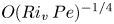 $O(Ri_v\,Pe)^{-{1}/{4}}$, the small-
 $Pe$ screening length in units of
 $a$. Although the existence of a rearward jet is well known for moderate Reynolds numbers from earlier computations (see Hanazaki, Kashimoto & Okamura Reference Hanazaki, Kashimoto and Okamura2009; Hanazaki, Nakamura & Yoshikawa Reference Hanazaki, Nakamura and Yoshikawa2015), its appearance has been attributed primarily to the inertial effects (for instance, see Eames & Hunt Reference Eames and Hunt1997); this belief, of the importance of inertia, has recently found explicit mention in Okino et al. (Reference Okino, Akiyama, Takagi and Hanazaki2021). The existence of such a jet in the Stokes stratification regime therefore comes as a surprise. It is also worth emphasizing that unlike the usual case of the laminar (or turbulent) wake or jet, the buoyant jet above does not conserve momentum flux; the implication of the jet region for the drift volume in a stratified fluid is discussed briefly in § 4.3.
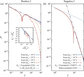
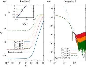
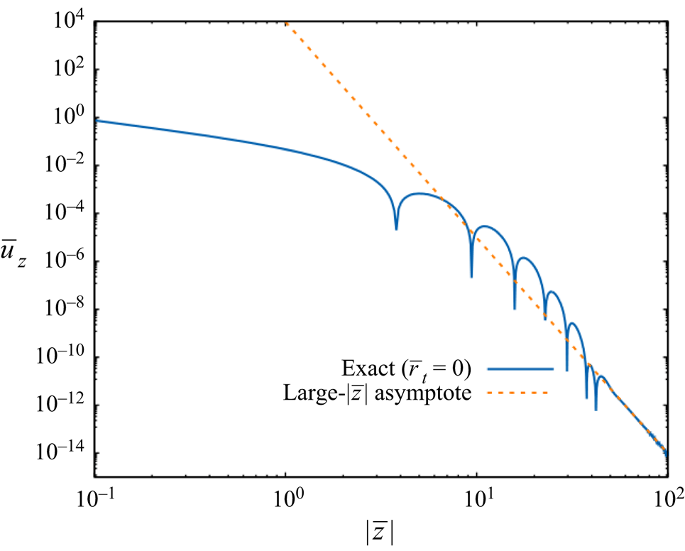
Figures 4 and 5 show plots of the axial velocity and density disturbance fields evaluated numerically at points along the stagnation streamline, based on (3.1) and (3.2), with  $\tilde {r}_t = 0$. Figure 4(b) shows the transition of the axial velocity field, for negative
 $\tilde {z}$, from an
 $O(1/\tilde {z})$ Stokeslet decay in the inner region to the more rapid
 $O(1/\tilde {z}^7)$ decay of the large-
 $\tilde {\eta }$ asymptote derived earlier (see § 3.1), on length scales greater than the (primary) screening length. Note that this transition is accompanied by a reversal in direction, as is evident from the sharp dip around
 $|\tilde {z}| \approx 8.85$ (
 $z \approx -8.85\,Ri_v^{-1/3}$) in the aforementioned logarithmic plot. Thus the axial flow in the neighbourhood of the front stagnation streamline, and at distances larger than the screening length, points towards the sphere. Importantly, the axial velocity profiles are virtually coincident for
 $\beta _\infty \leq 10^{-2}$, implying that the flow pattern in the vicinity of the front stagnation streamline converges to a limiting form for
 $Pe \rightarrow \infty$ that is characterized by the primary screening length of
 $O(Ri_v^{-{1}/{3}})$. In contrast, figure 4(a), for positive
 $\tilde {z}$, shows a transition from the inner region Stokeslet decay to an eventual exponential decay at the largest distances, with this transition being postponed to progressively larger
 $\tilde {z}$ with decreasing
 $\beta _\infty$. For the smallest
 $\beta _\infty$ values (
 $10^{-4}$ and
 $10^{-5}$), one can see the emergence of an intermediate asymptotic regime, corresponding to
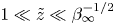 $1 \ll \tilde {z} \ll \beta _\infty ^{-{1}/{2}}$, where the velocity conforms to the reverse-Stokeslet behaviour predicted above. Note that both the Stokeslet and reverse-Stokeslet behaviours appear as the same asymptote (the black dot-dashed line), since the plot is for the absolute value of the velocity field on a logarithmic scale, and the indication of the reversal in direction is again the intervening sharp dip corresponding to
 $\tilde {z} \approx 1.15$ (
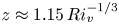 $z \approx 1.15\,Ri_v^{-{1}/{3}}$). The inset in this plot shows that the axial velocity profiles collapse onto a universal exponential behaviour when the ordinate and abscissa are rescaled with
 $\beta _\infty ^{{1}/{2}}$ and
 $\beta _\infty ^{-{1}/{2}}$, respectively, the latter corresponding to the axial distance being scaled by the secondary screening length. This collapse is consistent with (3.14), although since the distance corresponding to the reversal in direction scales with the primary screening length, the dips of the curves in the inset plot are no longer coincident for varying
 $\beta _\infty$.
The axial velocity field plotted along the stagnation streamline for both (a) positive  $\tilde {z}$ and (b) negative
 $\tilde {z}$, and for different small
 $\beta _\infty$. (a) Both the Stokeslet and reverse-Stokeslet asymptotes appear as the black dot-dashed line; the inset shows the collapse of the far-field profiles onto a common far-field decay, when plotted as a function of
 $\beta _\infty ^{{1}/{2}}\tilde {z}$, consistent with (3.14). (b) The transition from the near-field Stokeslet decay (blue dashed line) to the far-field decay given by
 $-{2160}/{\tilde {z}^7}$ (the black dot-dashed line).

The density disturbance field plotted along the stagnation streamline for both (a) positive  $\tilde {z}$ and (b) negative
 $\tilde {z}$, and for different small
 $\beta _\infty$. (a) The inset shows the collapse of the density disturbance profiles onto a common far-field asymptote, given by (3.15), when plotted as a function of
 $\beta _\infty ^{{1}/{2}}\tilde {z}$. (b) The small-
 $\beta _\infty$ density profiles converge to a common limiting form given by
 ${360}/{\tilde {z}^6}$; although in agreement with the far-field asymptote, the numerical approximations (with
 $N=150\,000$) break down for large axial distances, with this breakdown being delayed the most for
 $\beta _\infty = 10^{-2}$.

The plots in figure 5 again highlight the contrast between the density disturbance fields along the front and rear stagnation streamlines. Figure 5(b), for negative  $\tilde {z}$, shows that the density disturbance converges to a limiting form for
 $\beta _\infty \leq 10^{-2}$, with an
 $O(1/\tilde {z}^6)$ far-field decay, consistent with the large-
 $\tilde {\eta }$ asymptote obtained in § 3.1; although, the numerics break down beyond a certain
 $|\tilde z|$ that is a function of the number of quadrature points used. In contrast, figure 5(a) shows that the density disturbance transitions from a near-field plateau to a far-field exponential decay, with this plateau increasing in magnitude logarithmically with decreasing
 $\beta _\infty$, consistent with (3.15), and thereby precluding a collapse of the density profiles for small
 $\beta _\infty$. The inset plots the density profiles as a function of the rescaled abscissa,
 $\beta _\infty ^{{1}/{2}}\tilde {z}$, so as to highlight their collapse onto a common curve (the modified Bessel function asymptote given by (3.15)). The individual curves deviate from this common asymptote on account of the near-field plateauing behaviour, with this deviation occurring at a progressively smaller distance with decreasing
 $\beta _\infty$; for
 $\beta _\infty \rightarrow 0$, the said plateau regime becomes vanishingly small, while the exponential decay is pushed off to infinitely large distances (in units of the primary screening length), so the density field becomes logarithmically singular along the entire rear stagnation streamline. While the singularity itself is an expected consequence (for
 $Pe = \infty$) of the steady-state assumption, the nature of the divergence is an artefact of the outer-region analysis. The logarithmic singularity implies that the density disturbance, obtained from a time-dependent analysis, should diverge logarithmically for long times. However, as will be seen in Appendix D via simple physical arguments, the density along the rear stagnation streamline of a finite-sized sphere must instead diverge linearly in time, this divergence arising due to the asymptotically large residence time of fluid elements in the immediate neighbourhood of the rear stagnation point. There is no notion of a stagnation point in an outer-region analysis, and therefore, unlike the velocity field given by (3.14), the density field given by (3.15) is not valid exactly on the rear stagnation streamline (
 $\tilde {r}_t = r_t = 0$). One must instead interpret (3.15) as being valid for
 $\tilde {r}_t \ll 1$, but with
 $r_t$ still being much greater than
 $a$. The (negative) logarithmic divergence for
 $\beta _\infty \rightarrow 0$ can then be attributed to the logarithmically divergent (in time) downward drift displacements arising from the
 $O(1/z)$ Stokesian disturbance field.
3.3 Comparison of numerical profiles with the far-field approximations: transition from the jet to the wake regimes
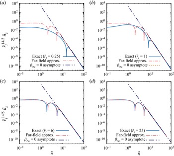
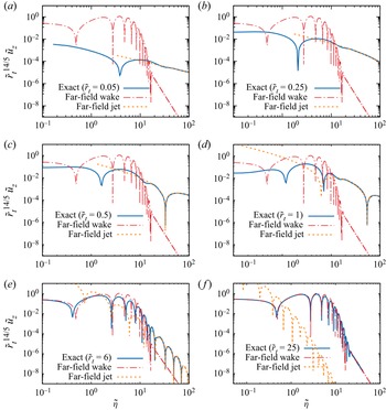
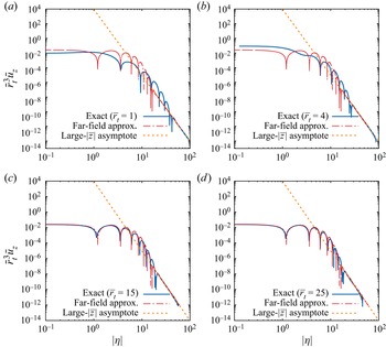
Having characterized the far-field approximations for the disturbance fields in both the buoyant jet (§ 3.2) and wake (§ 3.1) regions, we now compare the exact results for the axial velocity, obtained from a numerical evaluation of (3.1), for  $\beta _\infty = 10^{-5}$, with these approximations. The comparison is shown in figures 6 and 7 for negative and positive
 $\tilde \eta$, respectively. Motivated by the self-similar one-dimensional integral approximation given by (3.7), both figures plot
 $\bar {r}_t^{{14}/{5}}|\tilde {u}_z|$ as a function of
 $\tilde {\eta }$. Only the wake similarity profile (3.7) is relevant for negative
 $\tilde {\eta }$, and it is shown alongside the exact numerical profiles in figure 6 for different
 $\tilde {r}_t$, together with its large-
 $\tilde {\eta }$ asymptotic form given by
 $2160/\tilde {\eta }^7$. The agreement between the analytical and numerical profiles is poor for small to order unity
 $\tilde {r}_t$, with the number of zero-crossings also being in disagreement, but improves with increasing
 $\tilde {r}_t$. There is good agreement for
 $\tilde {r}_t = 6$, and almost a perfect match between the two sets of profiles for
 $\tilde {r}_t = 25$; an analogous comparison for the diffusion-dominant case is presented in Appendix A.
Comparison, for negative  $\tilde z$, between the numerically evaluated axial velocity profile and the far-field wake approximation given by (3.7), in the convection-dominant limit, and in the Stokes stratification regime (
 $Re \ll Ri_v^{{1}/{3}}$); the exact profile is obtained from a numerical integration of (3.1) with
 $\beta _\infty = 10^{-5}$.

Comparison, for positive  $\tilde z$, between the numerically evaluated axial velocity profile and the far-field jet and wake approximations given by (3.14) and (3.7), respectively. The profiles pertain to the convection-dominant limit and the Stokes stratification regime (
 $Re \ll Ri_v^{{1}/{3}}$); the numerical profile is obtained from an integration with
 $\beta _\infty = 10^{-5}$.

The comparison for positive  $\tilde {\eta }$ is more elaborate since one now has both far-field wake and jet approximations in different regions of the half-space. One expects the axial velocity profile to transition from a jet-like profile to a wake-like one as one moves away from the rear stagnation streamline, that is, for a fixed
 $\tilde {z}$ and with increasing
 $\tilde {r}_t$. This is seen in figure 7, where the numerically determined axial velocity profiles are shown for six different
 $\tilde {r}_t$ values ranging from
 $0.05$ to
 $25$, together with the far-field wake and jet approximations developed in the earlier two subsections. For the smallest
 $\tilde {r}_t (=0.05)$, the exact calculation matches the far-field jet approximation for
 $\tilde {z}$ greater than about
 $10$; for the chosen
 $\beta _\infty$, this jet approximation is virtually identical (in magnitude) to a Stokeslet decay over the range of
 $\tilde {\eta }$ examined. For the aforementioned
 $\tilde {r}_t$, similar to figure 4, the numerical profile has a zero-crossing at a smaller
 $\tilde {z} \approx 1.15$, and continues to diverge at smaller
 $\tilde {z}$, in accordance with the expected Stokeslet behaviour in the inner region, with the beginning of a plateau at the smallest
 $\tilde {z}$ values. For
 $\tilde {r}_t = 0.25$, the plateauing tendency for small
 $\tilde z$ is more readily evident, with there is still good agreement with the jet approximation for large
 $\tilde z$. The plateauing behaviour arises for any finite
 $\tilde {r}_t$ since the disturbance velocity field is now finite in the plane
 $\tilde {z} = 0$; the continued divergence down to
 $\tilde {z} = 0$ occurs only along the rear stagnation streamline (see figure 4). For
 $\tilde {r}_t$ values greater than unity, the exact profile starts to agree better with the wake approximation, and for
 $\tilde {r}_t=25$, this agreement is near perfect, with the jet approximation being virtually irrelevant. Although not shown, an analogous scenario prevails for the density disturbance profiles.
From figures 4 and 7, one sees that although the axial profile velocity exhibits only a single zero-crossing along the rear stagnation streamline (corresponding to the Stokeslet–reverse-Stokeslet transition for  $\beta _\infty = 0$), the jet approximation for any non-zero
 $\tilde {r}_t$ (see (3.12)) appears to exhibit multiple zero-crossings (likely a denumerable infinity of them) as is evident from the plots in the latter figure for
 $\tilde {r}_t = 6$ and
 $\tilde {r}_t = 25$. These zero-crossings suggest additional recirculating cells in the region
 $\tilde {z} \gg \tilde {r}_t$ for
 $\tilde {z},\tilde {r}_t \gg 1$. In fact, with
 $\beta _\infty = 0$ and
 $\hat {k}_t = k_t/\tilde {z}^{{1}/{2}}$ as a rescaled wavenumber, (3.12) is easily shown to be of the form
 $\tilde {z}^{-1}\,F(\tilde {r}_t \tilde {z}^{{1}/{2}})$, with
 $F$ having an oscillatory character, implying that the reverse Stokeslet identified above is only the central part of a far more elaborate axial flow structure behind the particle, one that exhibits multiple reversals as one proceeds outwards from the rear stagnation streamline, with successive reversals separated by a distance that decreases as
 $\tilde {z}^{-{1}/{2}}$. Note that this predominantly vertical flow structure is not in conflict with the finite number of zero-crossings predicted by the wake approximation, since the latter is restricted to the region
 $\tilde {z} \ll \tilde {r}_t$. Thus although the self-similar profiles in the wake predict an eventual algebraic decay, this decay might not extend to indefinitely large axial distances. Instead, with increasing
 $\tilde {z}$, one will again have zero-crossings in the region
 $\tilde {z}\gg \tilde {r}_t$. As of now, however, this is difficult to verify, given the near-impossibility of accurate numerical evaluation at such large distances. Nevertheless, and although not evident from figures 2 and 3, the implication is that the flow field in the convection-dominant limit exhibits an infinite number of recirculating cells; this is unlike the diffusion-dominant limit examined in Appendix A.
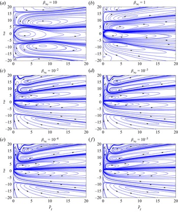
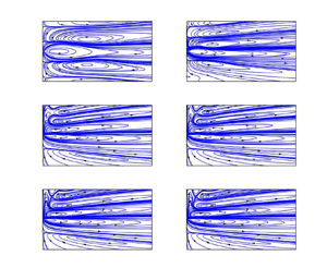
Finally, figures 8 and 9 show the streamline and isopycnal patterns, respectively, for  $\beta _\infty$ varying over the range
 $10^{-5}\unicode{x2013}10$. The departure of both patterns from fore–aft symmetry, with decreasing
 $\beta _\infty$, is evident, with the buoyant jet clearly evident in the streamline patterns for
 $\beta _\infty \leq 10^{-2}$. The spatial extent of all the streamline patterns shown corresponds to
 $|\tilde {z}|,\tilde {r} \leq 20$. For
 $\beta _\infty = 10^{-5}$, this implies that the streamline pattern includes the first two zero-crossings that appear in the large-
 $\tilde {r}_t$ axial velocity profile in figure 7, while including both zero-crossings that appear in the profiles in figure 6. Note that the length scale characterizing the streamline and isopycnal patterns changes from
 $Ri_v^{-{1}/{3}}$ to
 $(Ri_v\,Pe)^{-{1}/{4}}$ with increasing
 $\beta _\infty$. In units of
 $a\,Ri_v^{-{1}/{3}}$, this corresponds to the characteristic length scale increasing as
 $\beta _\infty ^{{1}/{4}}$. Thus for the same range in
 $\tilde {z}$ and
 $\tilde {r}_t$, one samples a proportionately smaller region of the streamline pattern with increasing
 $\beta _\infty$. This reduction in the spatial extent is evident from a comparison of the streamline pattern for
 $\beta _\infty = 10$ to the one in figure 12 (Appendix A). In figure 9, the isopycnals are seen to become heavily compressed and distorted for the smallest
 $\beta _\infty$ values, in a manner consistent with the density disturbance approaching being infinitely large (and negative) along the rear stagnation streamline (
 $\bar {r}_t = 0$,
 $\tilde {z} >0$), and as a result, numerically resolving the isopycnal becomes very difficult; this difficulty is reflected in the range of accessible
 $\tilde {r}_t$ and
 $\tilde {z}$ in figure 9 decreasing progressively with decreasing
 $\beta _\infty$ (this is not an issue for the streamline patterns, given that the axial velocity remains finite along the rear stagnation streamline even for
 $\beta _\infty = 0$).
Streamline patterns pertaining to the Stokes stratification regime (defined by the stratification screening length being the smallest of all relevant scales), for various  $\beta _\infty$. The plot for
 $\beta _\infty = 10$ is in the diffusion-dominant limit and nearly fore–aft symmetric; the plot for
 $\beta _\infty = 10^{-5}$ shows the buoyant reverse jet in the rear.

Isopycnals pertaining to the Stokes stratification regime, for various  $\beta _\infty$. The plot for
 $\beta _\infty = 10$ is in the diffusion-dominant limit and nearly fore–aft symmetric; the plots for the smallest
 $\beta _\infty$ values are suggestive of a developing singularity along the rear stagnation streamline.

3.4 Effects of weak inertia or convection
In our calculations thus far, we have completely neglected the role of inertia. This is equivalent to assuming the inertial screening length (of  $O(Re^{-1})$) to be much larger than the relevant stratification screening length, the latter being
 $(Ri_v\,Pe)^{-{1}/{4}}$ for
 $Pe \ll 1$ and
 $O(Ri_v^{-{1}/{3}})$ for
 $Pe \gg 1$, with this ordering of the screening lengths corresponding to the Stokes stratification regime. With regard to the calculations above, this is equivalent to setting
 $\alpha _0=0$ in (A2), and
 $\alpha _\infty =0$ in (2.7), for small and large
 $Pe$, respectively. While the detailed calculation of the flow field in the presence of competing effects of inertia and buoyancy is beyond the scope of the present paper, the effect of weak inertia on the larger-scale structure of the velocity field may nevertheless be inferred via scaling arguments.
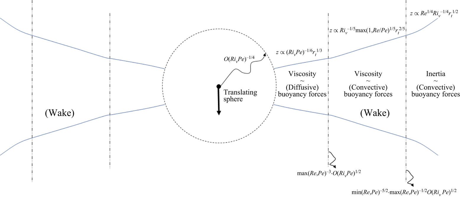
We begin with the diffusion-dominant case ( $Pe \ll 1$), where for small but finite
 $\alpha _0$ the denominator of the Fourier integrals for the disturbance fields, obtained from Fourier transforming (A1)–(A3), takes the form
 $\alpha _0\beta _0k_3^2k^2+\mathrm {i}k_3(\alpha _0+\beta _0)k^4+k^6+k_t^2$, with
 $k$ here being scaled by
 $(Ri_v\,Pe)^{{1}/{4}}$. Note that the term proportional to
 $\beta _0k_3k^4$ denotes effects arising from the (weak) convection of the density disturbance field, and is typically associated with a screening length of
 $O(Pe^{-1})$ (Leal Reference Leal2007); the fore–aft asymmetry in the far field arising from this term alone was already seen in the streamline and isopycnal patterns corresponding to the largest
 $\beta _\infty$ values in figures 8 and 9. Assuming buoyancy forces to first become important with increasing distance from the settling sphere, we now know from Appendix A that the dominant motion is restricted to an axisymmetric wake on distances greater than
 $O(Ri_v\,Pe)^{-{1}/{4}}$, and is primarily horizontal. Thus in order to examine inertia-induced transitions in the wake-scaling at larger distances, one may set
 $k_3 \gg k_t$, whence the aforementioned Fourier space expression takes the form
 $\alpha _0\beta _0k_3^4+\mathrm {i}(\alpha _0+\beta _0)k_3^5+k_3^6+k_t^2$. For
 $\alpha _0 = \beta _0 = 0$, one obtains the balance
 $k_3^6 \approx k_t^2$, and the vertical extent of the aforesaid wake grows as
 $z \propto (Ri_v\,Pe)^{-{1}/{6}}r_t^{{1}/{3}}$ (in units of
 $a$), as shown in Appendix A. For
 $\alpha _0, \beta _0$ small but finite, the neglected terms invariably become important, and balance buoyancy forces (instead of viscosity) on larger length scales, corresponding to smaller
 $k$ values. For
 $\alpha _0 \ll \beta _0$ (or
 $Re \ll Pe$), one obtains the balance
 $\beta _0 k_3^5 \approx k_t^2$ beyond a radial length scale of
 $O(Ri_v^{{1}/{2}}\,Pe^{-{5}/{2}})$; this balance is the same as that in § 3.1, and therefore implies a wake that grows as
 $z \propto Ri_v^{-{1}/{5}}\,r_t^{{2}/{5}}$. Thus even for
 $Pe \ll 1$, one obtains the large-
 $Pe$ wake-scaling derived in § 3.1, but only beyond the aforementioned secondary screening length. Note, however, that there is no buoyant jet on these scales, implying that the jet structure seen in figure 8(c) does not ‘come in’ from infinity with decreasing
 $\beta _\infty$. Finally, on the largest scales, the leading-order balance is between inertial and buoyancy forces, and takes the form
 $\alpha _0\beta _0 k_3^4 \approx k_t^2$, leading to a wake that grows as
 $z \propto Re^{{1}/{4}}\,Ri_v^{-{1}/{4}}\,r_t^{{1}/{2}}$ beyond a radial scale of
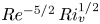 $Re^{-{5}/{2}}\,Ri_v^{{1}/{2}}$ that may be termed a tertiary screening length, again for
 $Re \ll Pe$. Thus in the diffusion-dominant limit, weak convection (small but finite
 $Pe$) and inertia effects (small but finite
 $Re$) alter the far-field wake-scaling, causing it grow progressively faster beyond the screening lengths obtained above. Although the difference in the growth exponents is marginal (
 $1/3 \rightarrow 2/5 \rightarrow 1/2$), one expects a more significant alteration of the wake structure; the change in structure accompanying the first transition in growth exponent (
 $1/3 \rightarrow 2/5$) involves a departure from fore–aft symmetry, and the details may already be inferred from §§ A.1 and 3.1. Provided that the stratification screening length
 $(Ri_v\,Pe)^{-{1}/{4}}$ remains the smallest of the three possible primary screening lengths, namely
 $(Ri_v\,Pe)^{-{1}/{4}}$,
 $Re^{-1}$ and
 $Pe^{-1}$, an assumption that defines the Stokes stratification regime for small
 $Pe$, the screening lengths derived above remain well-ordered under the assumption
 $Re \ll Pe$. If we allow for convection and inertial effects to be small but of comparable importance (
 $Re \sim Pe$), so that
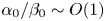 $\alpha _0/\beta _0 \sim O(1)$, then the growth exponents found above remain the same, but the secondary and tertiary screening lengths are now given by
 $\max (Re,Pe)^{-3}(Ri_v\,Pe)^{{1}/{2}}$ and
 $\min (Re,Pe)^{-5/2}\max (Re,Pe)^{-{1}/{2}}(Ri_v\,Pe)^{{1}/{2}}$. A schematic of the different wake-scaling regimes in the diffusion-dominant limit is given in figure 10; fluid motion outside the wake remains negligibly small.
Schematic of the different wake growth regimes in the diffusion-dominant limit ( $Pe \ll 1$).

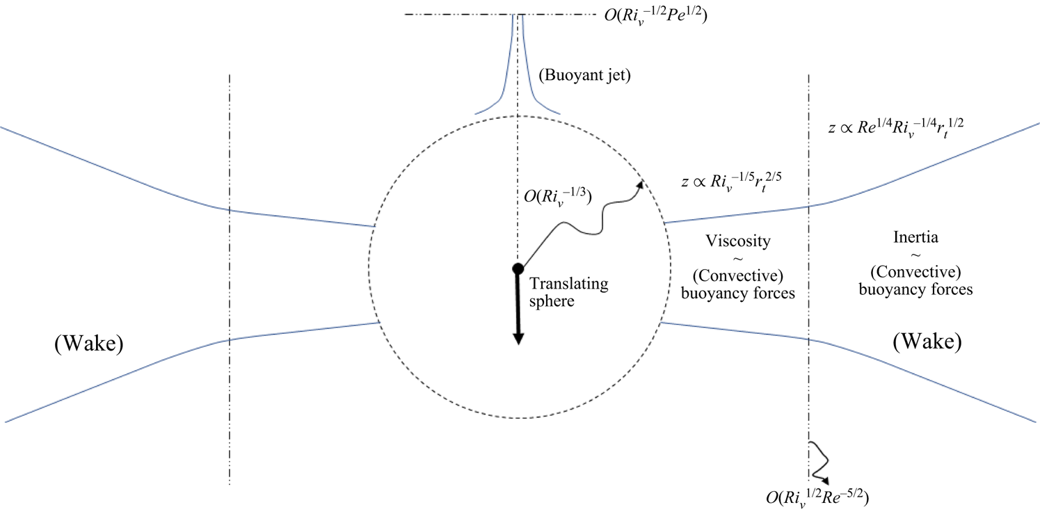
The effects of inertia in the convection-dominant limit, corresponding to  $Pe \gg 1$, are based on the same expression as that in the preceding paragraph, except that
 $k$ is now scaled with
 $Ri_v^{{1}/{3}}$, and accordingly, one has the form
 $-\alpha _\infty k_3^2 k^2+ {\rm i} \alpha _\infty \beta _\infty k_3k^4+\mathrm {i}k_3k^4+\beta _\infty k^6+k_t^2$. Outside of the buoyant jet, one may neglect
 $\beta _\infty k^6$ and use
 $k_3 \gg k_t$, implying the dominance of horizontal motion. Setting
 $\alpha _\infty = \beta _\infty = 0$ then leads to the balance
 $k_3^5 \approx k_t^2$, which, as already seen in § 3.1, and again in the analysis of the diffusion-dominant case above, yields the wake-scaling
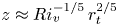 $z \approx Ri_v^{-{1}/{5}}\,r_t^{{2}/{5}}$. At length scales larger than a radial threshold of
 $O(Re^{-{5}/{2}}\,Ri_v^{{1}/{2}})$, the balance is between inertial and buoyancy forces, leading to the same square-root scaling
 $z \propto r_t^{{1}/{2}}$ seen above. Thus the difference with regard to the wake-scalings, in relation to the diffusion-dominant limit analysed above, is that the initial scaling regime
 $z \propto r_t^{{1}/{3}}$ is now absent, and one directly transitions to the
 $z \propto r_t^{{2}/{5}}$ scaling regime at distances much greater than the stratification screening length of
 $O(Ri_v^{-{1}/{3}})$. As already mentioned in § 3.2, a novel feature in the large-
 $Pe$ regime is the emergence of a buoyant jet that is smeared out by diffusion beyond a length scale of
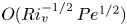 $O(Ri_v^{-{1}/{2}}\,Pe^{{1}/{2}})$. The diffusion-screening length for the jet is asymptotically smaller than the secondary screening length, of
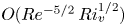 $O(Re^{-{5}/{2}}\,Ri_v^{{1}/{2}})$ above, provided that
 $Re\ll Ri_v^{{2}/{5}}\,Pe^{-{1}/{5}}$. A schematic of the various scaling regimes, in the convection-dominant limit, is given in figure 11.
Schematic of various regions in the convection-dominant limit for non-zero Reynolds and Péclet numbers in the Stokes stratification regime.

While the discussion in this paper has been restricted to the Stokes stratification regime, we mention briefly the screening lengths relevant to the inertia stratification regime that, for large  $Pe$, is defined by
 $Ri_v^{{1}/{3}} \ll Re$, or
 $\alpha _\infty \gg 1$; the inertial screening length of
 $O(Re^{-1})$ is now the primary screening length. For
 $Re \ll 1$, the fore–aft symmetric flow field in the inner Stokesian region first transitions, on scales of
 $O(Re^{-1})$, to a far-field structure consisting of an
 $O(1/r^2)$ source flow everywhere except for a viscous wake behind the translating sphere that acts as a directed sink (Batchelor Reference Batchelor1967; Subramanian Reference Subramanian2010). In terms of the Fourier space expression given in the preceding paragraph, the viscous wake corresponds to the balance
 $\mathrm {i}k_3k^4 \sim \alpha _\infty k_3^2 k^2$, leading to the familiar scaling
 $r_t \sim (z/Re)^{{1}/{2}}$ for the wake growth in physical space. This source-wake structure is expected to be modified by buoyancy forces when
 $k_t^2$ becomes comparable to the terms in the aforementioned balance. This happens for
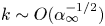 $k \sim O(\alpha _\infty ^{-{1}/{2}})$, which gives a secondary screening length of
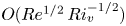 $O(Re^{{1}/{2}}\,Ri_v^{-{1}/{2}})$ in the inertia stratification regime (Zhang et al. Reference Zhang, Mercier and Magnaudet2019). The structure of the flow field on these length scales is currently under investigation.
4. Conclusions and discussion
4.1. Summary of main results
We have analysed in detail both the disturbance velocity and density fields induced by a sphere translating in a linearly stratified ambient fluid otherwise at rest. The analysis pertains to the Stokes stratification regime when buoyancy forces are dominant over inertial ones, so the transition from the well-known Stokesian behaviour, in the inner region, first occurs across a screening length determined by a balance between viscous and buoyancy forces. Our main focus is on the convection-dominant limit ( $Pe \gg 1$) when the screening length is
 $Ri_v^{-{1}/{3}}$. While we also analyse the diffusion-dominant limit in Appendix A, this has been the subject of earlier work (List Reference List1971; Ardekani & Stocker Reference Ardekani and Stocker2010), and our analysis is primarily for purposes of contrasting the nature of the fluid motion in the diffusion and convection-dominant limits.
In the aforementioned convection-dominant limit, and within the Stokes stratification regime defined by  $Re \ll Ri_v^{{1}/{3}} \ll 1$, we show through both computations (§ 3) and asymptotic analysis (§ 3.1) that the far-field fluid motion consists of an axisymmetric wake surrounding the sphere whose vertical extent grows as
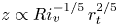 $z \propto Ri_v^{-{1}/{5}}\,r_t^{{2}/{5}}$, and wherein the fluid motion is predominantly horizontal. An analogue of this wake also exists in the diffusion-dominant limit (as explained in Appendix A), in which case it grows as
 $z \propto (Ri_v\,Pe)^{-{1}/{6}}\,r_t^{{1}/{3}}$, where
 $z$ and
 $r_t$ are here scaled by
 $a$. Although not obvious from the figures in earlier sections, the amplitude of fluid motion at a given non-dimensional distance (measured in units of the relevant screening length) is significantly greater for
 $Pe \gg 1$. In sharp contrast to the diffusion-dominant limit, we have shown (§ 3.2) that there also exists a buoyant reverse jet in the vicinity of the rear stagnation streamline for
 $Pe \gg 1$. Unlike the usual laminar or turbulent jets, which broaden with increasing distance downstream on account of the momentum flux being conserved, the buoyant jet region above narrows down with increasing distance downstream as
 $r_t \propto Ri_v^{-{1}/{6}}\,z^{-{1}/{2}}$, with a velocity field that, although oppositely directed, decays in the same manner as a Stokeslet for
 $Pe = \infty$; the jet is screened by diffusion beyond a length scale of
 $O(Ri_v^{-{1}/{2}}\, Pe^{{1}/{2}})$ for large but finite
 $Pe$. The recent effort of Shaik & Ardekani (Reference Shaik and Ardekani2020b) has investigated the flow pattern due to a towed (translating) particle in the aforementioned ‘convection-dominant’ limit, based on a numerical fast Fourier transform technique (figure 1a therein). Although the primary emphasis was on calculating the drift volume, their examination of the fluid motion shows the existence of a strong reverse flow along the rear stagnation streamline, beyond a threshold distance. This is broadly consistent with our findings, although there are quantitative discrepancies. Finally, in § 3.4, we comment briefly on the role of weak inertial (and convection) effects on the structure of the fluid motion beyond the primary buoyancy-induced screening length.
The fore–aft asymmetry of the large- $Pe$ disturbance velocity field found here has implications for pair interactions. A vertically oriented particle pair will experience a repulsive interaction for sufficiently large separations (on scales of
 $O(Ri_v^{-{1}/{3}})$). This is in contrast to the Stokesian scenario where the particle pair separation remains invariant with time, as may be established using reversibility arguments; note that the fore–aft symmetry of the
 $Pe = 0$ velocity field, obtained in Appendix A, implies that the particle pair separation, in a stratified fluid, is conserved to leading order in the diffusion-dominant limit. For
 $Pe \gg 1$, the aforementioned repulsive pair interaction is initially controlled by the greater magnitude of the velocity field along the front stagnation streamline, because the zero-crossing along the front stagnation streamline (
 $\approx 8.85\,Ri_v^{-{1}/{3}}$) occurs at a greater distance than that on the rear stagnation streamline (
 $\approx 1.15\,Ri_v^{-{1}/{3}}$). However, for distances a little beyond approximately
 $2\,Ri_v^{-{1}/{3}}$, the more rapid
 $O(1/z^7)$ decay of the disturbance velocity in front of the particle implies that the repulsion is controlled by the slowly decaying
 $O(1/z)$ disturbance along the rear stagnation streamline. Succinctly put, the rear particle pushes the one in front for smaller separations, while the opposite is true at larger separations. The range of repulsion is limited to a length scale of
 $O(Ri_v^{-{1}/{2}}\,Pe^{{1}/{2}})$ by the effects of diffusion. The above repulsive interaction is also in contrast to the homogeneous inertial case (
 $Re$ finite,
 $Ri_v = 0$), where the well-known drafting–kissing–tumbling scenario prevails, implying that a vertically oriented particle pair experiences an initial attraction (Joseph et al. Reference Joseph, Liu, Poletto and Feng1994). For a horizontally oriented particle pair in the large-
 $Pe$ limit, the inward radial velocities (not shown) imply an attractive interaction, again in contrast to the repulsion in the homogeneous inertial case (which leads to a self-similar expansion of sedimenting clusters; see Subramanian & Koch Reference Subramanian and Koch2008; Daniel et al. Reference Daniel, Ecke, Subramanian and Koch2009), but consistent with the recent work of Doostmohammadi & Ardekani (Reference Doostmohammadi and Ardekani2013) for a stratified medium, although the pair separations in this latter study were of
 $O(a)$. It is worth adding that the more complicated structure of the large-
 $Pe$ velocity field (see figure 8) implies that, unlike the homogeneous case, considering horizontal and vertically-aligned particle pairs alone does not really encompass the spectrum of pair interactions possible for other orientations.
4.2. Discussion: the inner-region scaling estimates
It was indicated in the Introduction as to how the validity of a linearized approximation is not obvious at large  $Pe$, given that the ambient isopycnals in the inner region are severely distorted by the sphere velocity field. An examination of the density disturbance in the inner region for large
 $Pe$ should help to identify possible restrictions on the results obtained in the paper, and a few comments in this regard are in order. We begin with the simpler case of small
 $Pe$ when the density perturbation around the sphere, on length scales of
 $O(a)$ (the inner region), quickly approaches a finite quasi-steady state for all subsequent times. The no-flux condition on the sphere surface causes the ambient isopycnals to tilt, so as to meet the sphere in a normal orientation. This tilting effect is significant in a region of
 $O(a^3)$, implying that the density perturbation associated with the aforementioned quasi-steady state is
 $O(\gamma a)$. The resulting baroclinically induced vorticity drives a flow of
 $O(\gamma a^3g/\mu )$, or
 $O(Ri_v)$ in non-dimensional terms (scaled by
 $U$; see Varanasi et al. Reference Varanasi, Marath and Subramanian2022). For
 $Ri_v \ll 1$, this weak flow may evidently be neglected compared to the primary Stokesian field. On larger length scales, convection of the base-state stratification by the perturbation Stokeslet field leads to a density perturbation that grows as
 $O(Pe\,r)$ in the inner region. The buoyancy forcing due to this density perturbation becomes comparable to viscous forces on length scales of
 $O(Ri_v\,Pe)^{-{1}/{4}}$, the small-
 $Pe$ stratification screening length identified first by List (Reference List1971) and Ardekani & Stocker (Reference Ardekani and Stocker2010); see also Appendix A. Importantly, for small
 $Pe$ and
 $Ri_v$, the Stokesian flow remains a valid leading-order approximation in the inner region for all times.
For large  $Pe$, the density perturbation in the inner region can become much larger than the nominal
 $O(\gamma a)$ estimate above. This may be seen by considering the limiting case of
 $Pe = \infty$, when the isopycnals are affinely convected by the sphere velocity field, there being no steady state. The sphere, as it settles through the stably stratified medium, continuously entrains positively buoyant fluid in a quasi-spherical annular region that extends behind it in a narrow wake that lengthens with time. The amplitude of the density perturbation near the sphere increases linearly with time as
 $O(\gamma Ut)$, leading to a buoyancy forcing per unit volume of
 $O(\gamma Ut g)$. Clearly, for large enough times, this buoyancy forcing will become comparable to the viscous terms even in the inner region, and for
 $Ri_v \ll 1$. Since the viscous terms in the equations of motion are
 $O({\mu U}/{a^2})$ in the inner region, the threshold time at which buoyancy forces are of a comparable magnitude is
 $O({\mu }/{\gamma a^2 g})$, or
 $O(({a}/{U})\,Ri_v^{-1})$. This is therefore the time at which the flow in the inner region must deviate from the leading Stokesian approximation on account of buoyancy forces; as mentioned in the Introduction, it is still possible for the structure of the fluid motion to remain similar to that detailed in this paper, but for a buoyancy-induced renormalization of the force exerted by the particle, although only a detailed examination of the inner region would confirm this. Moving to the outer region, in the Stokes stratification regime, the time scale associated with the development of the flow field in this region may be estimated as the time required for momentum to diffuse to a distance of
 $O(a\,Ri_v^{-1/3})$, which is
 $O(({a^2}/{\nu })\,Ri_v^{-2/3})$. The ratio of this latter time to the time scale estimated above, for the inner region to depart from a homogeneous Stokesian evolution, is
 $O(Re\,Ri_v^{1/3})$, and therefore, asymptotically small for
 $Re,Ri_v \ll 1$. Thus there is an asymptotically long interval of time corresponding to
 $({a^2}/{\nu })\,Ri_v^{-2/3} \ll t \ll ({a}/{U})\,Ri_v^{-1}$ where one has a quasi-steady response in the outer region, with the motion in the inner region still governed by the Stokes equations at leading order. The findings with regard to the nature of the fluid motion, detailed in § 3, are certainly valid in this time period. Note that for any finite
 $Pe$, however large, the distortion of the isopycnals will not continue indefinitely. Instead, there will eventually be a steady-state boundary layer, of thickness
 $O(a\,Pe^{-{1}/{3}})$, as far as the density gradient is concerned (although not for the density itself, which will continue to increase with time for an assumed constant
 $U$).
Scaling arguments similar to those in the preceding paragraph may also be used to assess the possibility of observing quasi-steady dynamics on scales beyond the primary screening length, and thereby to examine the relevance of the wake-scaling regimes sketched in § 3.4; see figures 10 and 11. Focusing on the Stokes stratification regime for large  $Pe$, the arguments in § 3.4 pointed to a secondary screening length of
 $O(a\,Re^{-{5}/{2}}\,Ri_v^{{1}/{2}})$ across which the dominant balance shifted from one between buoyancy and viscous forces to one between buoyancy and inertial forces. Given that the inertial forces enter the dominant balance, the time scale for a quasi-steady wake to be established on the aforementioned secondary screening length may be estimated as
 ${a\, Re^{-{5}/{2}}\,Ri_v^{{1}/{2}}}/{U}$. The ratio of this time scale to
 ${a\,Ri_v^{-1}}/{U}$ gives us
 $Re^{-{5}/{2}}\,Ri_v^{{3}/{2}}$, with this ratio needing to be much less than unity in order for a quasi-steady analysis of the fluid motion to hold; this yields
 $Re \gg Ri_v^{{3}/{5}}$. Combining this with the primary criterion for the large-
 $Pe$ Stokes stratification regime gives
 $Ri_v^{{3}/{5}} \ll Re \ll Ri_v^{{1}/{3}}$ for the dynamics in both the primary and secondary outer regions to be quasi-steady, in the time that the inner region has a Stokesian character.
4.3. Discussion: the drift volume scaling estimates
We now turn to the drift volume estimate for a sphere settling in a density stratified fluid, which, as mentioned in the Introduction, was one of the motivations for the analysis in this paper. The rapid algebraic decay of the far-field velocity disturbance, induced by buoyancy forces, implies that the drift volume  ${\mathcal {D}}$ will be finite in the presence of an ambient stratification, as argued originally by Subramanian (Reference Subramanian2010). More precise estimates for
 ${\mathcal {D}}$ as a function of
 $Ri_v$ and
 $Re$, in the Stokes and inertia stratification regimes, are obtained below. For the homogeneous Stokesian scenario, the
 $O(1/r)$ decay of the disturbance field implies a divergent drift volume for any finite time. As shown originally by Eames et al. (Reference Eames, Gobby and Dalziel2003), it therefore becomes necessary to define a partial drift volume
 ${\mathcal {D}}_p$ where, in contrast to Darwin (Reference Darwin1953), one considers only an initial material plane of a finite spatial extent. In a recent effort, Chisholm & Khair (Reference Chisholm and Khair2017) have shown that at leading order in
 $a/h$,
 ${\mathcal {D}}_p \sim ah^2 \sinh ^{-1} (Ut/h)$, where
 $t$ and
 $h$ here are the time and radius of the aforementioned material plane, respectively; the
 $h$-scaling clearly points to the finite-time divergence of
 ${\mathcal {D}} (= \lim _{h \rightarrow \infty } {\mathcal {D}}_p$) in the Stokesian limit. In the limits
 $Ut/h \ll 1$ and
 $Ut/h \gg 1$, the authors find
 ${\mathcal {D}}_p$ to be
 $O(ahUt)$ and
 $O[ah^2\ln (Ut/h)]$, respectively. These scalings may be obtained readily without a detailed calculation: for
 $Ut \ll h$, the flux through the original plane is independent of time, and due to the
 $U$-component of the Stokesian field, in the transverse plane containing the sphere. This component is
 $3Ua/(4r_t)$, and the flux through a circular section of radius
 $h$ is therefore given by
 $\int _0^h 3U(a/4r_t) 2{\rm \pi} r_t \,{\rm d}r_t \approx (3{\rm \pi} /2)Uah$, implying
 ${\mathcal {D}}_p \approx (3{\rm \pi} /2)Uah t$; here, the lower limit of the integral is taken to be
 $0$ since the leading contribution comes from
 $r_t$ of
 $O(h)$ (this is also the reason why a Stokeslet approximation suffices for the leading-order estimate). In the long-time limit of interest, when the distance of the material plane from the sphere is much larger than its radial extent, the flux is due primarily to the velocity
 $u_z \approx 3U/az$ along the rear stagnation streamline. The drift displacement due to this disturbance velocity field may be estimated as
 $\textstyle \int ^t {\rm d}t\,u_z = \int ^{Ut} ({\rm d}z'/U)u_z = \int ^{Ut} {\rm d}z'\,(3a/2z') \sim (3a/2)\ln (Ut)$, and is logarithmically divergent in time. A subtle point here is with regard to the argument of the logarithm; the approximate estimate above gives a dimensional argument for the logarithm, and one needs an additional length with respect to which
 $Ut$ in the logarithm is measured. Although an obvious choice would be
 $a$, the correct choice is
 $h$ (as is also evident from the exact result above), and this is because the onset of the logarithmic divergence is dependent on the transverse radial location of the fluid element. The decreasing magnitude of the disturbance field implies that it takes a progressively longer time for an element, further off from the translation axis, to be displaced through a distance of
 $O(a)$; evidently, the logarithmic divergence in time can begin only after the drift displacement has attained a magnitude of
 $O(a)$. For an element at a transverse distance of
 $O(h)$, the scale that contributes dominantly to
 ${\mathcal {D}}_p$ this time is
 $O(h/U)$, implying that the argument of the logarithm, in the expression for the drift displacement above, should be
 $t/(h/U)$; multiplication by
 ${\rm \pi} h^2$ gives the estimate
 ${\mathcal {D}}_p \approx ({3{\rm \pi} }/{2}) ah^2\ln (Ut/h)$.
In the Stokes stratification regime, one expects the dominant contribution to the drift volume to come from the range  $h \sim l_c$, where
 $l_c$ is the relevant stratification screening length;
 $l_c \sim O[(Ri_v\,Pe)^{-{1}/{4}}]$ for
 $Pe \ll 1$, and
 $O(Ri_v^{-{1}/{3}})$ for
 $Pe \gg 1$. However, for elements at these distances (from the translation axis), the drift displacement attains a magnitude of
 $O(a)$ only in the
 $O(l_c/U)$ time taken for the sphere to translate through a screening length. Since the velocity field decays faster for larger separations, there cannot be the analogue of the aforementioned logarithmic-in-time behaviour, for larger times, that occurred in the homogeneous case. This implies that
 ${\mathcal {D}}$ for the Stokes stratification regime can be obtained from the aforementioned long-time estimate for the Stokesian case by replacing
 $h$ with
 $l_c$, but removing the logarithm. One therefore obtains
 ${\mathcal {D}} \sim O[a^3(Ri_v\,Pe)^{-{1}/{2}}]$ and
 $O(a^3\,Ri_v^{-{2}/{3}}$), for small and large
 $Pe$, the latter estimate being relevant to the oceanic scenario (Katija & Dabiri Reference Katija and Dabiri2009; Subramanian Reference Subramanian2010); both estimates diverge in the limit of a homogeneous ambient (
 $Ri_v \rightarrow 0$), as must be the case. The numerical pre-factors in these estimates would require a detailed calculation of the drift displacements on length scales of order the stratification screening length. Note that fluid elements that start off at distances
 $h \ll l_c$ from the translation axis will suffer drift displacements of
 $O(a \ln Ri_v^{-{1}/{3}})$, and one therefore expects higher-order terms involving logarithms in a small
 $Ri_v$ expansion of
 ${\mathcal {D}}$ in the limit
 $Re \ll Ri_v^{{1}/{3}} \ll 1$. Recent efforts by Shaik & Ardekani (Reference Shaik and Ardekani2020a,Reference Shaik and Ardekanib) have obtained
 ${\mathcal {D}}_p$ numerically, in both the small and large
 $Pe$ limits. Consistent with the results of Chisholm & Khair (Reference Chisholm and Khair2017),
 ${\mathcal {D}}_p$ exhibits an
 $O(h^2)$ scaling with respect to the radial extent of the material plane under consideration. Further,
 ${\mathcal {D}}_p$ was found to increase logarithmically with
 $h/l_c$ in the limit
 $h/l_c \rightarrow 0$, this being consistent with logarithmic-in-time divergence in a homogeneous ambient being cut off for
 $t \sim O(l_c/U)$ (see, for instance, figure 5b in Shaik & Ardekani (Reference Shaik and Ardekani2020b)). The scaling arguments above imply that even the algebraic divergence of
 ${\mathcal {D}}_p$ with
 $h$ must be cut off once
 $h \sim O(l_c)$. Finally, it is also important to note that the narrowing down of the buoyant jet as
 $1/z^{{1}/{2}}$ with downstream distance implies that the
 $O(1/z)$ (reverse) Stokes-like decay of the axial velocity field within this jet region will not lead to divergent drift displacements, and therefore does not affect the above drift volume estimates.
In the inertia stratification regime ( $Ri_v^{{1}/{3}} \ll Re \ll 1$), discussed briefly towards the end of § 3.4, the disturbance velocity field attains the familiar source–sink structure on length scales larger than the primary (inertial) screening length of
 $O(a\,Re^{-1})$ (Batchelor Reference Batchelor1967). It is well known that the presence of a viscous wake leads to
 ${\mathcal {D}}$ diverging linearly in time for the homogeneous scenario (Subramanian Reference Subramanian2010; Chisholm & Khair Reference Chisholm and Khair2017). This divergence is seen readily from the constant flux through a fixed plane driven by the viscous wake. This flux is given by
 $u_z (r_t^{wake})^2$, where
 $r_t^{wake}\sim (az/Re)^{{1}/{2}}$, and is
 $O(Ua^2/Re)$, leading to
 ${\mathcal {D}} \sim (Ua^2/Re)t$ for the homogeneous case. For the stratified case, and for
 $Pe \gg 1$, this viscous wake persists only until the secondary screening length of
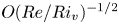 $O(Re/Ri_v)^{-{1}/{2}}$ obtained in § 3.4, and therefore the linear divergence above will be cut off for
 $t \sim O({a(Re/Ri_v)^{-{1}/{2}}}/{U})$, when stratification forces screen the wake velocity field, and one obtains
 ${\mathcal {D}} \sim a^3 (Re\,Ri_v)^{-{1}/{2}}$ in the inertia stratification regime. Note that this scaling is consistent with the scaling obtained above in the Stokes stratification regime, in that it reduces to
 $O(Ri_v^{-2/3})$ for
 $Re/Ri_v^{1/3} \sim O(1)$. In summary, for a fixed
 $Ri_v \ll 1$,
 ${\mathcal {D}}$ is expected to scale as
 $O(a^3\,Ri_v^{-{2}/{3}})$ until a
 $Re$ of
 $O(Ri_v^{{1}/{3}})$, decreasing thereafter as
 $O(a^3\,Re^{-{1}/{2}}\,Ri_v^{-{1}/{2}})$ for
 $Re \gg Ri_v^{{1}/{3}}$. A more detailed examination of pathlines and drift volume calculation to support the scaling arguments in this paragraph will be reported in a separate communication.
Acknowledgements
Numerical computations reported here were carried out using the Param Yukti facility provided under the National Supercomputing Mission, and the Nalanda-2 computational cluster available with JNCASR. The authors thank the institute for providing these facilities.
Declaration of interests
The authors report no conflict of interest.
Appendix A. Diffusion-dominant limit: analysis and results
Here, we present both numerical and analytical results pertaining to the velocity and density disturbance fields in the diffusion-dominant limit, corresponding to  $Pe = 0$. Although this limit has been examined earlier in the literature (List Reference List1971; Ardekani & Stocker Reference Ardekani and Stocker2010; Fouxon & Leshansky Reference Fouxon and Leshansky2014), the analysis below includes new results pertaining to the far-field disturbance decay, and the structure of the wake; importantly, the results here serve as a useful contrast to those obtained in the convection-dominant limit in the main text. We begin by obtaining the stratification-induced screening length in this limit.
For  $Pe \rightarrow 0$, the density perturbation on length scales of
 $O(1)$ arises from the no-flux boundary condition on the surface of the particle, and decays as
 $O({1}/{r^2})$ for
 $r \gg 1$. The convective correction to the density field satisfies
 $({1}/{Pe})\,\nabla ^2 \rho _f \sim (1-w)$; using
 $(1-w) \sim O({1}/{r})$ for the Stokeslet field leads to
 $\rho _f \sim Pe \, r$. The buoyancy forces arising from the convective perturbation grow as
 $O(Ri_v\,Pe\, r)$. Equating them to the decaying viscous forces of
 $O({1}/{r^3})$ leads to the small-
 $Pe$ stratification screening length
 $l_c \sim (Ri_v\,Pe)^{-{1}/{4}}$. The equations governing the disturbance fields on scales of order the aforementioned screening length may be obtained by using the expansions
 $\boldsymbol {u}=\boldsymbol {1}_z+(Ri_v\,Pe)^{1/4}\,\bar {\boldsymbol {u}}(\bar {\boldsymbol {r}})$,
 $p=p_{\infty }+(Ri_v\,Pe)^{{1}/{2}}\,\bar {p}(\bar {\boldsymbol {r}})$ and
 $\rho _f=Pe\,(Ri_v\,Pe)^{-{1}/{4}}\,\bar {\rho }_f(\bar {\boldsymbol {r}})$, with
 $\bar {\boldsymbol {r}}=(Ri_v\,Pe)^{{1}/{4}}{\boldsymbol r}$ being the scaled outer-region coordinate. Note that these scalings are based on the variation of the velocity, pressure and density disturbance as
 ${1}/{r}$,
 ${1}/{r^2}$ and
 $Pe\,r$, respectively, in the inner Stokesian region far away from the particle (that is, for
 $1 \ll r \ll (Ri_v\,Pe)^{-{1}/{4}}$). The outer-region equations are given by
 \begin{gather} \bar{\boldsymbol{\nabla}}\boldsymbol{\cdot} \bar{\boldsymbol{u}}=0, \end{gather}
 \begin{gather}-\alpha_0\,\frac{\partial \bar{\boldsymbol{u}}}{\partial \bar z}={-}\bar{\boldsymbol{\nabla}} \bar p +\bar \nabla^2 \bar{\boldsymbol{u}}-[\bar{\rho}_f+6{\rm \pi}\,\delta(\bar{\boldsymbol{r}})]\,\boldsymbol{1}_{\boldsymbol{z}}, \end{gather}
 \begin{gather}-\boldsymbol{1}_{\boldsymbol{z}}\boldsymbol{\cdot}\bar u+\beta_0\, \frac{\partial\bar{\rho}_f}{\partial \bar z} = \bar \nabla^2 \bar{\rho}_f. \end{gather}
Here,  $\alpha _0$ and
 $\beta _0$ are given by
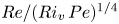 ${Re}/{(Ri_v\,Pe)^{1/4}}$ and
 ${Pe}/{(Ri_v\,Pe)^{1/4}}$, respectively, and denote the ratios of the small-
 $Pe$ stratification screening length to the inertial (
 $Re^{-1}$) and convective (
 $Pe^{-1}$) screening lengths. Similar to the large-
 $Pe$ case in § 2, the boundary condition on the particle surface has been replaced by a point force on the right-hand side of (A2). For
 $Pe,Re \ll (Ri_v\,Pe)^{{1}/{4}}$, one may ignore the terms proportional to
 $\alpha _0$ and
 $\beta _0$, with the velocity and density disturbance fields reducing to the following Fourier integrals:
 \begin{gather} \bar{\boldsymbol{u}} (\bar{\boldsymbol{r}}) = \frac{-3}{4{\rm \pi}^2} \int \frac{k^4 (\boldsymbol{1}_{\boldsymbol{z}}-k_3\boldsymbol{k}/k^2)}{k^6+k_t^2} \,{\rm e}^{{\rm i}\boldsymbol{k}\boldsymbol{\cdot}\bar{\boldsymbol{r}}} \,{\rm d}\boldsymbol{k}, \end{gather}
 \begin{gather}{\bar{\rho}_f}(\bar{\boldsymbol{r}}) = \frac{-3}{4{\rm \pi}^2} \int \frac{k_t^2}{k^6+k_t^2} \,{\rm e}^{{\rm i}\boldsymbol{k}\boldsymbol{\cdot}\bar{\boldsymbol{r}}} \,{\rm d}\boldsymbol{k}. \end{gather}
List (Reference List1971) used residue theory to enable the reduction of (A4) and (A5) to one-dimensional integrals for both the two- and three-dimensional cases. We use a different method that reduces the disturbance fields to two-dimensional integrals instead, this being conveniently applicable in both the diffusion-dominant and convection-dominant limits. Thus, similar to § 2, (A4) and (A5) are expressed in a spherical coordinate system with its polar axis aligned with the translation direction, the integral over the azimuthal angle ( $\phi$) then being carried out analytically, with the resulting expressions given by
 \begin{gather} \bar{u}_{z}=\frac{-3(2+bar{r}_t^2/\bar{z}^2)}{4\,|\bar{z}|\,(1+\bar{r}_t^2/\bar{z}^2)^{{3}/{2}}} +\frac{3}{2{\rm \pi}}\int_0^\infty {\rm d}k \int_0^{\rm \pi} {\rm d}\theta\,\frac{\sin^5\theta\, J_0(k\bar{r}_t\sin \theta)\cos(k\bar{z}\cos\theta)}{k^4+\sin^2\theta}, \end{gather}
 \begin{gather}\bar{\rho}_{f}=\frac{-3}{2{\rm \pi}}\int_0^\infty {\rm d}k \int_0^{\rm \pi} {\rm d}\theta\,\frac{k^2\sin^3 \theta\,J_0(k\bar{r}_t\sin \theta)\,{\rm e}^{{\rm i}k\bar{z}\cos\theta}}{k^4+\sin^2\theta}. \end{gather}
Note that for reasons already mentioned in § 2, the Stokeslet contribution in (A6) has been separated out to aid the numerical evaluation of the second integral term. The associated Stokes streamfunction is given by
 \begin{equation} \boldsymbol{\bar{\psi}}_s=\frac{-3\bar{r}_t^2}{4(\bar{r}_t^2+\bar{z}^2)^{{1}/{2}}} +\frac{3\bar{r}_t}{2{\rm \pi}}\int_0^\infty {\rm d}k \int_0^{\rm \pi} {\rm d}\theta\,\frac{\sin^4\theta\,J_1(k\bar{r}_t\sin \theta)\cos(k\bar{z}\cos\theta)}{k(k^4+\sin^2\theta)}. \end{equation}
The density disturbance and axial velocity fields, and the Stokes streamfunction, given by (A7), (A6) and (A8), respectively, are evaluated using Gaussian quadrature. The instantaneous streamline and isopycnal patterns, in a reference frame with a far-field quiescent ambient, are shown in figure 12, and are seen to be fore–aft symmetric, as may also be inferred from the cosine in (A6) and (A8). As found originally by List (Reference List1971) and Ardekani & Stocker (Reference Ardekani and Stocker2010), buoyancy forces suppress the long-range vertical motion associated with the Stokeslet at distances of  $O(Ri_v\,Pe)^{-{1}/{4}}$, leading to the development of recirculating cells aligned with the direction of stratification, and wherein the motion is predominantly horizontal.
(a) Streamlines and (b) isopycnals, for a translating sphere in a linearly stratified fluid in the diffusion-dominant limit ( $Pe = 0$). In the point-particle approximation used, the sphere is at the origin and moving vertically downwards.

A.1. Far-field analysis
At distances large compared to  $(Ri_v\,Pe)^{-{1}/{4}}$, one expects largely horizontal motion, as is evident from the rather small aspect ratios of the recirculating cells in figure 12(a). This translates to the assumption
 $k_3 \gg k_t$ in Fourier space, and the Fourier integrals in (A4) and (A5) take the following simplified forms:
 \begin{gather} \bar{\boldsymbol{u}} (\bar{\boldsymbol{r}}) ={-}\frac{3}{4{\rm \pi}^2}\int \frac{k^4 (\boldsymbol{1}_{\boldsymbol{z}}-k_3\boldsymbol{k}/k^2)}{k_3^6+k_t^2} \,{\rm e}^{{\rm i}\boldsymbol{k}\boldsymbol{\cdot}\bar{\boldsymbol{r}}} \,{\rm d}\boldsymbol{k}, \end{gather}
 \begin{gather}\bar{\rho}_f (\bar{\boldsymbol{r}}) ={-}\frac{3}{4{\rm \pi}^2}\int \frac{k_t^2}{k_3^6+k_t^2} \,{\rm e}^{{\rm i}\boldsymbol{k}\boldsymbol{\cdot}\bar{\boldsymbol{r}}} \,{\rm d}\boldsymbol{k}. \end{gather}
In a cylindrical coordinate system aligned with the translation direction, and after carrying out the  $\phi$ integration, the axial and radial velocity components, and the density field, are given by
 \begin{gather} \bar{u}_{z}=\frac{-3}{2{\rm \pi}}\int_{-\infty}^\infty {\rm d}k_3 \int_0^\infty {\rm d}k_t\, \frac{k_3^2k_t^3\, J_0(k_t\bar{r}_t)\,{\rm e}^{{\rm i}k_3\bar{z}}}{k_3^6+k_t^2}, \end{gather}
 \begin{gather}\bar{u}_{r_t}=\frac{3i}{2{\rm \pi}}\int_{-\infty}^\infty {\rm d}k_3 \int_0^\infty {\rm d}k_t\, \frac{k_3^3k_t^2\, J_1(k_t\bar{r}_t)\,{\rm e}^{{\rm i}k_3\bar{z}}}{k_3^6+k_t^2}, \end{gather}
 \begin{gather}\bar{\rho}_{f_1}=\frac{-3}{2{\rm \pi}}\int_{-\infty}^{\infty} {\rm d}k_3 \int_0^\infty {\rm d}k_t\, \frac{k_t^3\,J_0(k_t\bar{r}_t)\,{\rm e}^{{\rm i}k_3\bar{z}}}{k_3^6+k_t^2}. \end{gather}
Next, one uses contour integration to evaluate the  $k_3$ integral. Contributions arise from the existence of six poles in the complex-
 $k_3$ plane, with these poles being symmetrically disposed about the real
 $k_3$-axis, consistent with the fore–aft symmetry of the disturbance fields. The contour integration yields the following one-dimensional integrals:
 \begin{gather} \bar{u}_{z}={-}3{\rm i}\int_0^\infty k_t^2\,J_0(k_t \bar{r}_t)\,(lq_1^2\,{\rm e}^{{\rm i} q_1 k_t^{{1}/{3}} |\bar{z}|}+mq_2^2\,{\rm e}^{{\rm i} q_2 k_t^{{1}/{3}} |\bar{z}|}+nq_3^2 \,{\rm e}^{{\rm i} q_3 k_t^{{1}/{3}} |\bar{z}|})\,{\rm d}k_t, \end{gather}
 \begin{gather}\bar{u}_{{r_t}}={-}3{\rm sgn}{\bar{z}} \int_0^\infty k_t^{{4}/{3}}\,J_1(k_t \bar{r}_t)\,(lq_1^3 \,{\rm e}^{{\rm i} q_1 k_t^{{1}/{3}} |\bar{z}|}+mq_2^3 \,{\rm e}^{{\rm i} q_2 k_t^{{1}/{3}} |\bar{z}|}+nq_3^3 \,{\rm e}^{{\rm i} q_3 k_t^{{1}/{3}} |\bar{z}|})\,{\rm d}k_t, \end{gather}
 \begin{gather}\bar{\rho}_{f}={-}3{\rm i}\int_0^\infty k_t^{{4}/{3}}\,J_0(k_t \bar{r}_t)\,(l \,{\rm e}^{{\rm i} q_1 k_t^{{1}/{3}} |\bar{z}|}+m \,{\rm e}^{{\rm i} q_2 k_t^{{1}/{3}} |\bar{z}|}+n \,{\rm e}^{{\rm i} q_3 k_t^{{1}/{3}} |\bar{z}|})\,{\rm d}k_t. \end{gather}
Here,  $q_1$,
 $q_2$,
 $q_3$,
 $l$,
 $m$ and
 $n$ are complex-valued constants given by
 \begin{gather} [q_1,q_2,q_3,q_4,q_5,q_6]=[{\rm e}^{{{\rm \pi} {\rm i}}/{6}}, {\rm e}^{{{\rm \pi} {\rm i}}/{2}},{\rm e}^{{5 {\rm \pi}{\rm i}}/{6}}, {\rm e}^{{7 {\rm \pi}{\rm i}}/{6}}, {\rm e}^{{9 {\rm \pi}{\rm i}}/{6}},{\rm e}^{{11 {\rm \pi}{\rm i}}/{6}}], \end{gather}
 \begin{gather}l=\frac{1}{(q_1-q_2)(q_1-q_3)(q_1-q_4)(q_1-q_5)(q_1-q_6)}, \end{gather}
 \begin{gather}m=\frac{1}{(q_2-q_1)(q_2-q_3)(q_2-q_4)(q_2-q_5)(q_2-q_6)}, \end{gather}
 \begin{gather}n=\frac{1}{(q_3-q_1)(q_3-q_2)(q_3-q_4)(q_3-q_5)(q_3-q_6)}. \end{gather}
Setting  $(k_t\bar {r}_t)^{{1}/{3}} = p$ as the integration variable, and using
 $\bar {\eta }={\bar {z}}/{\bar {r}_t^{{1}/{3}}}$, with some simplification, yields
 \begin{gather} \bar{u}_{z}=\frac{-9{\rm i}}{\bar{r}_t^3}\int_0^\infty p^8\,J_0(p^3)\,(lq_1^2\,{\rm e}^{{\rm i}q_1p|\bar{\eta}|}+mq_2^2\,{\rm e}^{{\rm i}q_2p|\bar{\eta}|}+nq_3^2\,{\rm e}^{{\rm i}q_3p|\bar{\eta}|})\,{\rm d}p, \end{gather}
 \begin{gather}\bar{\rho}_{f}=\frac{-9{\rm i}}{\bar{r}_t^{7/3}}\int_0^\infty p^6\,J_0(p^3)\,(l\,{\rm e}^{{\rm i}q_1p|\bar{\eta}|}+m\,{\rm e}^{{\rm i}q_2p|\bar{\eta}|}+n\,{\rm e}^{{\rm i}q_3p|\bar{\eta}|})\,{\rm d}p, \end{gather}
 \begin{gather}\bar{u}_{{r_t}}=\frac{-9{\rm sgn}(\eta)}{\bar{r}_t^{7/3}}\int_0^\infty p^6\, J_1(p^3)\,(lq_1^3\,{\rm e}^{{\rm i}q_1p|\bar{\eta}|}+mq_2^3\,{\rm e}^{{\rm i}q_2p|\bar{\eta}|}+nq_3^3\,{\rm e}^{{\rm i}q_3p|\bar{\eta}|})\,{\rm d}p. \end{gather}
The above self-similar forms point to a thin axisymmetric wake bracketing the horizontal plane containing the settling sphere, in the far field, whose vertical extent grows as  $z \propto (Ri_v\,Pe)^{-{1}/{6}}\,{r}_t^{{1}/{3}}$, where
 $z$ and
 $r_t$ are now in units of
 $a$; the self-similarity is also evident from figure 12, where the number and shapes of recirculating cells is invariant for large
 $r_t$, with their vertical extents alone increasing with increasing
 $r_t$. Even within the self-similar wake, it can be seen from (A21)–(A23) that the disturbance fields decay more rapidly compared to the
 $O(1/r)$ decay of the Stokeslet, reinforcing the fact that buoyancy forces screen the originally long-ranged Stokesian fields. The one-dimensional integrals in (A21)–(A23) are readily evaluated numerically, and furthermore, the large-
 $\bar {\eta }$ asymptotes, obtained from using the small-argument approximation for the Bessel function, are given by
 $\bar {u}_{z}\approx {181\,440}/{(\bar {r}_t^3|\bar {\eta }|^9)}$,
 $\bar {u}_{{r_t}}\approx {\rm sgn}(\eta )\,({816\,480}/{(\bar {r}_t^{7/3}|\bar {\eta }|^{10})})$, and
 $\bar {\rho }_{f}\approx {-3240}/{(\bar {r}_t^{7/3}|\bar {\eta }|^{7})}$.
The comparison between one-dimensional profiles of the axial velocity field, obtained from the exact calculations above (which led to the streamline pattern in figure 12), and those obtained from the far-field self-similar approximation given by (A21) is shown in figure 13 for various  $\bar {r}_t$ values. The plots correspond to
 $\bar {r}_t^3 \bar {u}_z$ as functions of
 $|\eta |$, as a result of which the far-field approximation shown remains invariant to a change in
 $\bar {r}_t$. In the log-log plots shown, the zero-crossings of the axial velocity (which correlate roughly to the boundaries between recirculating cells) appear as sharp dips (to negative infinity). There exist significant differences between the numerical and far-field predictions for
 $\bar {r}_t$ values of order unity; for instance, the number of zero-crossings in the numerical field depends on
 $\bar {r}_t$, being
 $7$ for
 $\bar {r}_t=1$,
 $6$ for
 $\bar {r}_t=4$, and increasing to
 $8$ (the same as the far-field approximation) for
 $\bar {r}_t \geq 15$. The agreement improves with increasing
 $\bar {r}_t$, and there is near-quantitative agreement for the largest
 $\bar {r}_t\ (=25)$; note that the streamline pattern in figure 12(a) includes only three of the eight zero-crossings for
 $\bar {r}_t = 25$. Finally, for
 $\bar {r}_t$ values greater than that corresponding to the final zero-crossing, the axial velocity profiles conform to the algebraic asymptote above, namely
 $\bar {r}_t^3\bar {u}_{z}\approx {181\,440}/{|\bar {\eta }|^9}$, shown as the dashed orange line in figure 13. An analogous scenario prevails for the density disturbance field.
The axial velocity profiles in the diffusion-dominant limit ( $Pe = 0$): comparison between the exact numerical profiles and the far-field approximation given by (A21) for various
 $\bar {r}_t$ values. The large-
 $\bar {\eta }$ analytical asymptote is shown as a dashed orange line.

As one approaches the translation axis (the stagnation streamline corresponding to  $\bar {r}_t=0$),
 $\bar {\eta }$ becomes asymptotically large for any finite
 $\bar {z}$, and only the large-
 $\bar {\eta }$ asymptotes are of relevance. On substituting for
 $\bar {\eta }$, the large-
 $\bar {\eta }$ asymptotes for the axial velocity and density fields above are seen to be functions of only
 $|\bar {z}|$, suggesting that these asymptotes remain valid far-field (large-
 $|\bar {z}|$) approximations even along the translation axis. The radial velocity is, of course, zero along the stagnation streamline, with the large-
 $\bar {\eta }$ approximation above being
 $O(\bar {r}_t)$ for small
 $\bar {r}_t$. In figure 14, we compare the exact axial velocity field for
 $\bar {r}_t = 0$, again obtained numerically, with the large-
 $\bar {\eta }$ asymptote that is now proportional to
 $\bar {z}^{-9}$. Although the locations of the (seven) zero-crossings of the exact profile can no longer be predicted, the far-field algebraic decay nevertheless conforms to the asymptote above. For
 $\bar {r}_t = 0$ alone, the velocity field given by (2.11) is expressible in terms of a one-dimensional integral that again yields the aforementioned large-
 $\bar {z}$ asymptote (Fouxon & Leshansky Reference Fouxon and Leshansky2014).
Axial velocity, as a function of  $|\bar {z}|$, for
 $\bar {r}_t = 0$ (the translation axis), in the diffusion-dominant limit (
 $Pe = 0$). The large-
 $\bar {z}$ asymptote is shown as a dashed orange line.

Appendix B. The far-field wake velocity and density fields in the convection-dominant ( $Pe \rightarrow \infty$ or $\beta _\infty \rightarrow 0$) limit


We again start with the expressions appropriate for the far-field wake, given by (A9) and (A10), where the approximation of nearly horizontal motion has been made. In a cylindrical coordinate system aligned with the translation direction, and after carrying out the  $\phi$ integration, the expressions for the axial and transverse velocities, and the density disturbance, reduce to
 \begin{gather} \bar{u}_{z}=\frac{-3{\rm i}}{2{\rm \pi}}\int_{-\infty}^\infty {\rm d}k_3 \int_0^\infty {\rm d}k_t\, \frac{k_3k_t^3\, J_0(k_t\bar{r}_t)\,{\rm e}^{{\rm i}k_3\bar{z}}}{{\rm i}k_3^5+k_t^2}, \end{gather}
 \begin{gather}\bar{u}_{r_t}=\frac{3{\rm i}}{2{\rm \pi}}\int_{-\infty}^\infty {\rm d}k_3 \int_0^\infty {\rm d}k_t\, \frac{k_3^2k_t^2\, J_1(k_t\bar{r}_t)\,{\rm e}^{{\rm i}k_3\bar{z}}}{{\rm i}k_3^5+k_t^2}, \end{gather}
 \begin{gather}\bar{\rho}_{f_1}=\frac{-3}{2{\rm \pi}}\int_{-\infty}^{\infty} {\rm d}k_3 \int_0^\infty {\rm d}k_t\, \frac{k_t^3\,J_0(k_t\bar{r}_t)\,{\rm e}^{{\rm i}k_3\bar{z}}}{{\rm i}k_3^5+k_t^2}. \end{gather}
As for the diffusion-dominant case analysed in Appendix A, the next step is to evaluate the  $k_3$ integral using contour integration. There now exist five poles in the complex-
 $k_3$ plane, with two poles in the lower half and three poles in the upper half of the complex plane; the differing number of poles in the two halves of the plane translates to fore–aft asymmetry of the axial velocity and density disturbance fields. The residue integration then yields the following one-dimensional integrals for positive and negative
 $\tilde {z}$:
 \begin{align} \tilde{u}_{z}&=\begin{cases} {-3}{\rm i}\displaystyle\int_0^\infty k_t^{9/5}\,J_0[k_tr_t]\,[Q_1q_1\,{\rm e}^{{\rm i}q_1k_t^{{2}/{5}}\tilde{z}}+Q_2q_2\,{\rm e}^{{\rm i}q_2k_t^{{2}/{5}}\tilde{z}}+Q_3q_3\,{\rm e}^{{\rm i}q_3k_t^{{2}/{5}}\tilde{z}}]\,{\rm d}k_t & (\textrm{for } \tilde z>0), \\ 3{\rm i}\displaystyle\int_0^\infty k_t^{9/5}\,J_0[k_tr_t]\,[Q_4q_4\,{\rm e}^{{\rm i}q_4k_t^{{2}/{5}}\tilde{z}}+Q_5q_5\,{\rm e}^{{\rm i}q_5k_t^{{2}/{5}}\tilde{z}}]\,{\rm d}k_t & (\textrm{for } \tilde z<0),\end{cases} \end{align}
 \begin{align} \tilde{\rho}_{f}&=\begin{cases} {-3}\displaystyle\int_0^\infty k_t^{7/5}\,J_0[k_tr_t]\,[Q_1\,{\rm e}^{{\rm i}q_1k_t^{{2}/{5}}\tilde{z}}+Q_2\,{\rm e}^{{\rm i}q_2k_t^{{2}/{5}}\tilde{z}}+Q_3\,{\rm e}^{{\rm i}q_3k_t^{{2}/{5}}\tilde{z}}]\,{\rm d}k_t & (\textrm{for } \tilde z>0), \\ 3\displaystyle\int_0^\infty k_t^{7/5}\,J_0[k_tr_t]\,[Q_4\,{\rm e}^{{\rm i}q_4k_t^{{2}/{5}}\tilde{z}}+Q_5\,{\rm e}^{{\rm i}q_5k_t^{{2}/{5}}\tilde{z}}]\,{\rm d}k_t & (\textrm{for } \tilde z<0),\end{cases} \end{align}
 \begin{align} \tilde{u}_{r_t}&=\begin{cases} {-3}\displaystyle\int_0^\infty k_t^{6/5}\,J_0[k_tr_t]\,[Q_1q_1^2\,{\rm e}^{{\rm i}q_1k_t^{{2}/{5}}\tilde{z}}+Q_2q_2^2\,{\rm e}^{{\rm i}q_2k_t^{{2}/{5}}\tilde{z}}+Q_3q_3^2\,{\rm e}^{{\rm i}q_3k_t^{{2}/{5}}\tilde{z}}]\,{\rm d}k_t & (\textrm{for } \tilde z>0), \\ 3\displaystyle\int_0^\infty k_t^{6/5}\,J_0[k_tr_t]\,[Q_4q_4^2\,{\rm e}^{{\rm i}q_4k_t^{{2}/{5}}\tilde{z}}+Q_5q_5^2\,{\rm e}^{{\rm i}q_5k_t^{{2}/{5}}\tilde{z}}]\,{\rm d}k_t & (\textrm{for } \tilde z<0).\end{cases} \end{align}
Here,  $q_1$,
 $q_2$,
 $q_3$,
 $q_4$,
 $q_5$,
 $Q_1$,
 $Q_2$,
 $Q_3$,
 $Q_4$ and
 $Q_5$ are complex-valued constants given by
 \begin{gather} [q_1,q_2,q_3,q_4,q_5]=[{\rm e}^{{{\rm \pi} {\rm i}}/{10}}, {\rm e}^{{{\rm \pi} {\rm i}}/{2}},{\rm e}^{{9 {\rm \pi}{\rm i}}/{10}}, {\rm e}^{-{7 {\rm \pi}{\rm i}}/{10}}, {\rm e}^{-{3 {\rm \pi}{\rm i}}/{10}}], \end{gather}
 \begin{gather}Q_1=\frac{1}{(q_1-q_2)(q_1-q_3)(q_1-q_4)(q_1-q_5)}, \end{gather}
 \begin{gather}Q_2= \frac{1}{(q_2-q_1)(q_2-q_3)(q_2-q_4)(q_2-q_5)}, \end{gather}
 \begin{gather}Q_3= \frac{1}{(q_3-q_1)(q_3-q_2)(q_3-q_4)(q_3-q_5)}, \end{gather}
 \begin{gather}Q_4= \frac{1}{(q_4-q_1)(q_4-q_2)(q_4-q_3)(q_4-q_5)}, \end{gather}
 \begin{gather}Q_5= \frac{1}{(q_5-q_1)(q_5-q_2)(q_5-q_3)(q_5-q_4)}. \end{gather}
Setting  $k_t\bar {r}_t = p$ as the integration variable, and using
 $\tilde {\eta }={\tilde {z}}/{\tilde {r}_t^{{2}/{5}}}$, yields (3.7), (3.8) and (3.9).
Appendix C. Effects of diffusion and quadrature points on the fields
The rationale behind the retention of weak diffusion effects (small but finite  $\beta _\infty$) is illustrated in figure 15, where we compare the numerically evaluated axial velocity profiles at
 $r_t=25$ for
 $\beta _\infty = 0$ and
 $10^{-5}$ for varying numbers of quadrature points. The
 $\beta _\infty = 0$ profile deviates from the true profile, asymptoting instead to a spurious plateau beyond a certain
 $\tilde {z}$. Further, there is only a modest effect of quadrature resolution on this threshold
 $\tilde {z}$, and as a result, for
 $\beta _\infty = 0$, the eventual algebraic decay regime remains numerically inaccessible regardless of the number of quadrature points. On the other hand, the profile for
 $\beta _\infty = 10^{-5}$ does access the algebraic decay regime, and the numerical error does reduce with increase (from 30 000 to 50 000) in the number of quadrature points.
The comparison given highlights the importance of weak diffusive effects (small but finite  $\beta _\infty$) in obtaining an accurate representation of the disturbance fields in the convection-dominant limit. The profiles for
 $\beta _\infty = 0$ asymptote to a spurious plateau regardless of
 $N$; here,
 $N$ represents the number of quadrature points used for numerical integration. The axial velocity calculations shown here are performed for
 $r_t=25$.

Appendix D. The density disturbance field along the rear stagnation streamline for $Pe = \infty$

Any fluid element on the rear stagnation streamline that starts off at a finite distance behind the particle, at  $t = 0$, will end up infinitely far behind it for
 $t \rightarrow \infty$. In the laboratory reference frame, this may be attributed to the fluid element being either pushed up (for sufficiently large distances) or dragged down by a velocity disturbance that is smaller (in magnitude) than the particle translation velocity. Thus, in a reference frame moving with the particle, fluid elements at any finite distance along the rear stagnation streamline, for
 $t \rightarrow \infty$, must have started in an infinitesimally small neighbourhood of the rear stagnation point at
 $t = 0$. The downward distances travelled by these fluid elements and the particle must both diverge linearly in time, at leading order, for
 $t \rightarrow \infty$. Since for
 $Pe = \infty$ each fluid element carries the density value corresponding to its initial location, the ambient linear stratification implies that the density disturbance at the locations of these fluid elements must also diverge (to negative infinity) linearly in time.
We now obtain the above linear-in-time divergence of the disturbance density field, for  $Pe = \infty$, in a more formal manner, starting from the advection equation in the laboratory reference frame
 $(\hat {z},t)$ given by
 \begin{equation} \frac{\partial \rho_f}{\partial t} + u_z(\hat{z},t)\,\frac{\partial \rho_f}{\partial \hat{z}} = 0 \end{equation}
along the rear stagnation streamline, with  $u_z$ being time-dependent on account of the changing position of the translating spherical particle. In the particle-fixed reference frame
 $(z,t)$, with vertical coordinate
 $z = \hat {z} + Ut$, one may write
 \begin{equation} \frac{\partial \rho'_f}{\partial t} + (U+u_z')\,\frac{\partial \rho'_f}{\partial z} = \gamma u'_z \end{equation}
in terms of the disturbance velocity and density fields (note that (D2) includes the nonlinear convective contribution). An analytically simple representation of the zero- $\beta _\infty$ velocity field found in the text may be taken as
 $u'_z = -{Ua}/{z} + ({2Ua}/{z})\,{\mathcal {H}}(z - 1.15 a\,Ri_v^{-{1}/{3}})$ which includes the Stokeslet–reverse-Stokeslet transition across a threshold downstream distance (
 $1.15 a\,Ri_v^{-{1}/{3}}$); here,
 ${\mathcal {H}}(x)$ is the Heaviside function. One solves (D2) for
 $\rho '_f$ in the region
 $z \geq a$, with
 $z = a$ corresponding to the rear stagnation point. Note that unlike a translating particle, the above model velocity field only has a Stokeslet term in the inner region (
 $r \sim O(a)$), and is therefore more representative of a translating bubble. As a result, the total velocity field
 $U+ u_z'$ goes to zero linearly for
 $z \rightarrow a^+$, instead of the quadratic scaling behaviour expected in the neighbourhood of a no-slip surface. This does not affect the long-time behaviour of the density disturbance, however, as should also be evident from the arguments in the previous paragraph. As a final simplification, we retain only the Stokeslet component of the disturbance velocity in the convective term on the left-hand side of (D2), which retains the essential ingredient of the velocity going to zero at the rear stagnation point; the neglect of the reverse Stokeslet contribution in the convecting velocity field is of no consequence since the dominant convection is by the ambient flow
 $U$ for
 $z \gg O(a)$.
Defining the scaled variables  $\tilde {z} = z/a\,Ri_v^{-{1}/{3}}$,
 $\tilde {t} = t/(a\,Ri_v^{-{1}/{3}}/U)$, and using the scale
 $\gamma a$ for
 $\rho '_f$ (while continuing to use the same symbol), one obtains
 \begin{equation} \frac{\partial \rho'_f}{\partial \tilde{t}} + \left(1-\frac{Ri_v^{{1}/{3}}}{\tilde{z}}\right)\frac{\partial \rho'_f}{\partial \tilde{z}} ={-}\frac{1}{\tilde{z}} + \frac{2}{\tilde{z}}\,{\mathcal{H}}(\tilde{z} - 1.15), \end{equation}
with  $\tilde {z} = Ri_v^{{1}/{3}}$ now denoting the scaled stagnation point coordinate. One now defines the convected coordinate via the relation
 ${{\rm d}\tilde {z}}/{{\rm d}t} = 1 - {Ri_v^{{1}/{3}}}/{\tilde {z}}$, which may be solved to obtain
 \begin{equation} \tilde{z} - \tilde{z}_0 + Ri_v^{{1}/{3}} \ln \frac{\tilde{z} - Ri_v^{{1}/{3}}}{\tilde{z}_0 - Ri_v^{{1}/{3}}} = \tilde{t}, \end{equation}
where  $\tilde {z}_0$ denotes the initial position of the fluid element, and serves as the convected coordinate. Although not lending itself to an explicit inversion, (D4) may nevertheless be understood as follows. For small times
 $\tilde {t} \ll Ri_v^{{1}/{3}}$, for fluid elements starting close to the rear stagnation point (
 $\tilde {z}_0 \approx Ri_v^{{1}/{3}}$), the logarithmic term is dominant and one obtains
 $\tilde {z} - Ri_v^{{1}/{3}} \approx (\tilde {z}_0 - Ri_v^{{1}/{3}}) \,{\rm e}^{Ri_v^{-{1}/{3}}\tilde {t}}$, corresponding to the initial exponential increase in distance from the rear stagnation point under the action of a linear extensional flow. For
 $\tilde {t} \gg Ri_v^{{1}/{3}}$,
 $\tilde {z} \approx \tilde {t} - Ri_v^{{1}/{3}}\ln \tilde {t} + Ri_v^{{1}/{3}} \ln (\tilde {z}_0 - Ri_v^{{1}/{3}})$, the linear increase at leading order corresponding to convection by the ambient uniform flow. From both the short- and long-time approximations, one sees that
 $\tilde {t} \rightarrow \infty$ for
 $\tilde {z}_0 \rightarrow Ri_v^{{1}/{3}}$ with
 $\tilde {z}$ finite – that is, the time required to traverse a finite distance, along the rear stagnation streamline, diverges with increasing vicinity to the rear stagnation point.
Having clarified the nature of the convected coordinate, we transform from  $(\tilde {z},\tilde {t})$ to
 $(\tilde {z}_0,t)$, with the functional form
 $\tilde {z}(\tilde {z}_0,\tilde {t})$ being defined implicitly by (D4). The left-hand side of (D2) now takes the form of a partial time derivative, and one may readily write the formal solution for the density disturbance as
 \begin{equation} \rho'_f(\tilde{z}_0,t) = \int_0^{\tilde{t}}\left[ - \frac{1}{\tilde{z}(\tilde{z}_0,\tilde{t}')} + \frac{2}{\tilde{z}(\tilde{z}_0,\tilde{t}')}\,{\mathcal{H}}(\tilde{z}(\tilde{z}_0,\tilde{t}')-1.15)\right] {\rm d}\tilde{t}'. \end{equation}
Although this integral cannot be evaluated analytically owing to the absence of an explicit expression for  $\tilde {z}(\tilde {z}_0,\tilde {t})$, simplifications are possible for the limit of interest:
 $\tilde {t} \gg 1$ with
 $\tilde {z}$ finite. In the said limit,
 $\tilde {z}_0 \rightarrow Ri_v^{{1}/{3}}$, and the long-time approximation takes the form
 $\tilde {z}(\tilde {z}_0,\tilde {t}) \approx \tilde {t} + Ri_v^{{1}/{3}} \ln (\tilde {z}_0 -Ri_v^{{1}/{3}})$. One may use this approximation to evaluate the second integral in (D5) as
 \begin{equation} \int_0^{\tilde{t}} \frac{2}{\tilde{z}(\tilde{z}_0,\tilde{t}')}\,{\mathcal{H}}(\tilde{z}(\tilde{z}_0,\tilde{t}')-1.15) \,{\rm d}\tilde{t}' =\int_{\tilde{t}^*}^{\tilde{t}} \frac{2}{\tilde{t}'+ Ri_v^{{1}/{3}}\ln (\tilde{z}_0 - Ri_v^{{1}/{3}})} \,{\rm d}\tilde{t}', \end{equation}
where  $\tilde {t}^* = 1.15 - Ri_v^{{1}/{3}} \ln (\tilde {z}_0 -Ri_v^{{1}/{3}})$. On evaluation, one obtains
 $2 \ln (\tilde {z}/1.15)$ provided that
 $\tilde {z} > 1.15$ (
 $\tilde {t} > \tilde {t}^*$), and zero otherwise. Importantly, this second integral is seen to evaluate to a finite value in the long-time limit, in the particle-fixed reference frame. Note that one may also interpret the above contribution in the laboratory reference frame: since the laboratory coordinate (
 $\hat {z}$) corresponds to
 $\tilde {z}$ in the above logarithm, increasingly linearly with
 $t$, the second integral now contributes to a positive
 $\rho _f'$ that diverges for
 $t \rightarrow \infty$, this being consistent with the positive and logarithmically divergent drift displacement suffered by any fluid element, for sufficiently long times, on account of the reverse-Stokeslet region along the rear stagnation streamline.
Now we consider the first integral in (D5). The dominant contribution to this integral comes from the vicinity of the rear stagnation point, and to illustrate the long-time divergence, it is sufficient to assume  $\tilde {z}$ to be at a small but fixed distance away from the stagnation point. This assumption is not a limiting one, since it takes only a finite time for the fluid element to be convected to any other larger
 $\tilde {z}$; the ambient uniform flow starts to be dominant for such
 $\tilde {z}$, and would lead to an additional contribution proportional to
 $-\ln \tilde {z}$. Neglecting this latter logarithmic contribution, and using the invert corresponding to the short-time approximation in the first integral, (D5) takes the form
 \begin{equation} \rho'_f(\tilde{z}_0,t) ={-} \int_0^t {\rm d}t'\,\frac{1}{[Ri_v^{{1}/{3}} + (\tilde{z}_0 - Ri_v^{{1}/{3}}) \,{\rm e}^{Ri_v^{-{1}/{3}} t'}]}, \end{equation}
where the second integral in (D5) is neglected on account of the small- $\tilde {z}$ assumption. On integrating, one obtains
 \begin{equation} \rho'_f(\tilde{z}_0,t) =\ln \left[ \frac{Ri_v^{{1}/{3}}\,{\rm e}^{{-}Ri_v^{-{1}/{3}} t} + (\tilde{z}_0 - Ri_v^{{1}/{3}})}{z_0} \right], \end{equation}
or, rewriting in terms of  $\tilde {z}$,
 \begin{equation} \rho'_f(\tilde{z},t) =\ln \left[ \frac{z}{Ri_v^{{1}/{3}}\,{\rm e}^{Ri_v^{-{1}/{3}} t} + (\tilde{z} - Ri_v^{{1}/{3}})} \right]. \end{equation}
For finite  $\tilde {z}$ and
 $t \rightarrow \infty$, one has
 $\rho '_f \approx -\ln (Ri_v^{{1}/{3}}\, {\rm e}^{Ri_v^{-{1}/{3}} t}) \approx - t$, the expected linear growth in time.