1. Introduction
Shock-wave/boundary-layer interaction (SWBLI) has been the subject of many studies during the last 60 years (Dolling Reference Dolling2001). Three configurations are commonly studied: the case of a compression ramp; the oblique shock impinging on a flat-plate boundary layer; and the normal shock on a wall (or profile). The latter configuration, which is the focus of the current study, is common in air intakes, nozzle exits or in transonic flow over aerofoils.
Regardless of the configuration, many experimental and numerical studies have shown the coexistence of two distinct characteristic frequencies: shock motions involve low frequencies, while the mixing layer downstream of the separation exhibits unsteadiness whose frequencies are higher than those observed in the shock motions, but are still below the energetic scales of incoming turbulence. Inside the recirculation bubble both motions are at play. Turbulent boundary layer fluctuations are referred to as high-frequency unsteadiness.
As commonly done in SWBLI (Erengil & Dolling Reference Erengil and Dolling1991b
), one can introduce a dimensionless frequency (or Strouhal number) defined as
 $St_{L}=fL_{int}/U_{e}$
where
 $U_{e}$
is the external velocity and
 $L_{int}$
is the interaction length scale. Using this scaling, Dussauge, Dupont & Debiève (Reference Dussauge, Dupont and Debiève2006) have shown that a value of
 $St_{L}=0.02{-}0.05$
characterises the shock motions in several configurations. Concerning medium-frequency motions in the mixing layer, typical values spanning
 $St_{L}=0.1$
to
 $St_{L}=0.5$
are common for shock-induced separations. Those motions have been associated to Kelvin–Helmholtz instabilities, which can generate a vortex shedding phenomenon.
The origin of low-frequency motions affecting shock waves is controversial. One of the first answers was suggested by Plotkin (Reference Plotkin1975), who developed a mathematical model where the shock foot is affected by the passage of turbulent eddies, while the ‘stability’ of the mean flow tends to restore the shock to its original position. The hypothesis of shock motions caused by organised structures in the incoming flow has been assessed by several experimental investigations: Andreopoulos & Muck (Reference Andreopoulos and Muck1987) found that the frequency of the shock unsteadiness is of the same order as the bursting frequency of the upstream boundary layer. Subsequently, Erengil & Dolling (Reference Erengil and Dolling1991a ) and Dolling & Erengil (Reference Dolling and Erengil1991) found correlations between pressure fluctuations in the upstream boundary layer and the shock velocity, but in a more recent study Beresh, Clemens & Dolling (Reference Beresh, Clemens and Dolling2002) suggest that a thickening/thinning boundary layer is not the cause of the shock unsteadiness, and that shock motions are inherited from eddies in the incoming flow.
While the shock is undoubtedly affected by the passage of low- or high-speed perturbations, upstream events might be only one of several causes of shock unsteadiness. To prove it, Touber & Sandham (Reference Touber and Sandham2009) performed large-eddy simulations (LES) in a shock-reflection configuration, where special care was devoted to prevent the development of coherent structures in the incoming flow. Low-frequency shock motions could still be observed. Dupont, Haddad & Debiève (Reference Dupont, Haddad and Debiève2006) also found very weak coherence between the pressure fluctuations in the upstream boundary layer and those at the shock foot. On the contrary, fluctuations at the shock were strongly correlated with the separated zone. According to those studies, low-frequency oscillations are not caused by incoming turbulent eddies, but by the coupling between the dynamics of the separated zone and the shock, either through global instability of the separation bubble, or through some mechanism of self-sustainment.
The two theories described above, even if in disagreement on the location, support the idea that the instability is driven by a unique source. However, a plausible model is that the interaction responds as a dynamical system which is forced by external disturbances (Clemens & Narayanaswamy Reference Clemens and Narayanaswamy2014). In this respect, Touber & Sandham (Reference Touber and Sandham2011) proposed an original derivation of the Plotkin (Reference Plotkin1975) equation and stated that the low-frequency unsteadiness was related to a fundamental property of the shock wave. The model combines numerical evidence and analytical theory to prove that the coupling between the shock and the boundary layer is mathematically equivalent to a first-order low-pass filter: low-frequency unsteadiness is not caused by a forcing, either from upstream or downstream of the shock, but is an intrinsic property of the global system.
Linear stability analysis has become a tool commonly used in fluid dynamics, which can often help to understand flow unsteadiness (Sipp et al. Reference Sipp, Marquet, Meliga and Barbagallo2010; Theofilis Reference Theofilis2011). According to Huerre (Reference Huerre, Batchelor, Moffatt and Worster2000), occurrences of unsteadiness can be classified into two main categories: the flow can behave as an oscillator, with an absolute instability imposing its own dynamics, or as a noise-amplifier, if the system filters and amplifies existing environmental noise. In the first case, a global-mode decomposition has the ability to identify the mechanism responsible for the self-sustained unsteadiness. Otherwise the unsteadiness is characterised by a broadband spectrum and requires an external forcing to persist. The flow does not exhibit any unstable global mode and the linearised Navier–Stokes operator acts as a linear filter of the upstream disturbance environment. In such cases a singular-value decomposition of the Navier–Stokes or the resolvent operators highlights optimal growth or pseudo-resonance phenomena (Trefethen et al. Reference Trefethen, Trefethen, Reddy and Driscoll1993; Schmid & Henningson Reference Schmid and Henningson2001). The connection between transient growth and convective instability has been discussed by Cossu & Chomaz (Reference Cossu and Chomaz1997) and numerous studies have successfully applied these methods to different configurations (Ehrenstein & Gallaire Reference Ehrenstein and Gallaire2005; Abdessemed et al. Reference Abdessemed, Sharma, Sherwin and Theofilis2009; Alizard, Cherubini & Robinet Reference Alizard, Cherubini and Robinet2009; Brandt et al. Reference Brandt, Sipp, Pralits and Marquet2011).
In SWBLI, only few studies have tried to answer the question of the origins of the unsteadiness through stability analyses. In a laminar interaction, Robinet (Reference Robinet2007) found an unstable global mode. However, the mode was three-dimensional and non-oscillatory and cannot therefore account for the low-frequency shock oscillations. In a transonic flow over a profile, Crouch et al. (Reference Crouch, Garbaruk, Magidov and Travin2009) and Sartor, Mettot & Sipp (Reference Sartor, Mettot and Sipp2015) showed that an unstable global mode appears at a critical value of the angle of attack (or Mach number), above which the shock starts to oscillate. Also, it was found that the oscillation frequency accurately matches the global mode frequency. This picture is similar to the case of vortex shedding in a cylinder wake (Jackson Reference Jackson1987) and may be described as a Hopf bifurcation. In a shock impinging on a turbulent boundary layer configuration, Touber & Sandham (Reference Touber and Sandham2009) performed a global-mode decomposition of a mean flow obtained by time- and span-averaging of a three-dimensional LES computation. The most unstable global mode was stationary, so the result cannot be considered as relevant to explain flow unsteadiness. Following a similar approach, Pirozzoli et al. (Reference Pirozzoli, Larsson, Nichols, Bernardini, Morgan and Lele2010) confirmed the presence of a non-oscillatory exponentially growing mode, but documented also the presence of slightly damped oscillatory eigenvalues. Those modes, even if stable, display frequencies comparable to the unsteadiness observed in full LES.
These partial results indicate that the interaction dynamics could be captured by a linear stability analysis. Yet an eigenvalue decomposition may not be the correct approach. If the interaction behaves as a noise amplifier, then the unsteady behaviour of the flow could be better characterised by an input/output analysis focusing on the receptivity of the flow to external forcing. In separation bubbles, the existence of optimal growth phenomena has been proven by Marquet et al. (Reference Marquet, Sipp, Chomaz and Jacquin2008) and Blackburn, Barkley & Sherwin (Reference Blackburn, Barkley and Sherwin2008), who described the flow dynamics by determining the optimal initial perturbations which maximise the energy gain over a given time horizon. In configurations where there is a strong frequency-selection process, working in the frequency instead of the temporal domain has a deeper physical meaning (Farrell & Ioannou Reference Farrell and Ioannou1996). Hence, following Alizard et al. (Reference Alizard, Cherubini and Robinet2009) and Cerqueira & Sipp (Reference Cerqueira and Sipp2014), the existence of pseudo-resonances in a given frequency range may explain the existence of a peak in the frequency spectrum of an unsteady flow. A singular-value decomposition of the resolvent operator may be able to identify these pseudo-resonances. The outcome of such an analysis yields for all frequencies an optimal gain, an optimal forcing and an optimal response. The peaks of the optimal gain curve may then correspond to the preferred frequencies of the flow, the structure of the optimal response to the structure of the flow unsteadiness, while the spatial structure of the optimal forcing may indicate where upstream noise or turbulence could optimally trigger this perturbation. This approach has already been used to describe the most amplified modes in a channel flow configuration (Jovanovic & Bamieh Reference Jovanovic and Bamieh2005), in a turbulent pipe flow (McKeon & Sharma Reference McKeon and Sharma2010) and in a Blasius boundary layer (Brandt et al. Reference Brandt, Sipp, Pralits and Marquet2011).
Linear stability analyses are rigorous and widely used in the case of laminar, transitional flows. Extension to turbulent flows is not straightforward (Mettot, Sipp & Bézard Reference Mettot, Sipp and Bézard2014b ). In the case of turbulent flows for which the scale decoupling assumption holds (Rodi Reference Rodi1997; Iaccarino et al. Reference Iaccarino, Ooi, Durbin and Behnia2003; Lawson & Barakos Reference Lawson and Barakos2011), the dynamics of the large scales of the flow may be captured using unsteady Reynolds-averaged Navier–Stokes (RANS) equations. The impact of the small scale dynamics on the large ones is accounted for by a turbulence model, which results in an additional viscosity (eddy viscosity). Stability analyses involving the linearization of the full RANS equations have already successfully been performed in the case of transonic flow over a profile (Crouch et al. Reference Crouch, Garbaruk, Magidov and Travin2009; Sartor et al. Reference Sartor, Mettot and Sipp2015) or open cavity flow (Mettot, Renac & Sipp Reference Mettot, Renac and Sipp2014a ). Both configurations exhibit well-defined peaks in the frequency spectrum linked to the existence of a globally unstable mode. In the present article, we will follow this line of thought and assume that the above-mentioned low- and medium-frequencies of the SWBLI are captured by time integration, while the high-frequency motions are taken into account by the turbulence model.
In this work, we propose to characterise the unsteadiness of the well-documented transonic SWBLI over the Délery bump (Délery Reference Délery1978; Bur et al. Reference Bur, Benay, Galli and Berthouze2006). We will compare experimental measurements to linear stability analyses. First (§ 2), the frequency selection process is highlighted using wall-pressure and skin-friction measurements. Then, Fourier-mode decompositions of Schlieren photography reveal the spatial location of low- and medium-frequency unsteadiness, whilst cross-correlation maps illustrate their spatial structures. Second (§ 3), we will perform linear stability analyses of a mean-flow obtained by a RANS approach. After a brief presentation of the stability approaches and of the discretisation choices, we will discuss the results of the global-mode decomposition – the eigenvalues of the full linearised RANS equations – and those of the singular-value decomposition of the resolvent. We will assess the ability of stability both approaches to predict the flow unsteadiness observed experimentally.
2. Experimental investigation
The experiments were conducted in the S8Ch transonic wind tunnel of the ONERA Meudon centre, a continuous open-loop facility supplied with desiccated atmospheric air. Total pressure and temperature were near ambient conditions:
 $p_{st}=0.96\times 10^{5}\pm 300$
Pa and
 $T_{st}=300\pm 10$
K. The unit Reynolds number is around
 $Re=14\times 10^{6}~\text{m}^{-1}$
, which leads to a value of
 $Re_{{\it\Theta}}=3500$
for the incoming boundary layer. An air dryer is placed after the air inlet to control the flow humidity: during every test, the temperature rise was lower than
 $2\,^{\circ }\text{C}$
, and the dew point is maintained around
 $-50\,^{\circ }\text{C}$
.
The transonic S8Ch wind tunnel in the ONERA Meudon centre. (a) Photo of the test section. (b) Schematic diagram.

The test section (figure 1) has a span of
 $100\times 120$
mm and its lower wall is a profile designed to produce a uniform supersonic flow. A second throat of adjustable cross section is placed at the outlet and causes by choking effect a shock wave whose position and intensity can be adjusted in a continuous manner. The ratio between the two sections is 1.12, and the shock occurs at Mach number
 $Ma=1.4$
outside the interaction region.
Two-component laser Doppler velocimetry (LDV) measurements performed in the same configuration and facility (Bur, Corbel & Délery Reference Bur, Corbel and Délery1998; Bur, Coponet & Carpels Reference Bur, Coponet and Carpels2009) have shown that upstream of the shock, the boundary layer on the bump is fully turbulent with a physical thickness
 ${\it\delta}=4$
mm and a momentum thickness
 ${\it\Theta}=0.25$
mm. The shock position is monitored by the evolution of static pressure through 36 pressure taps on the lower wall (see figure 12
b). The mean velocity field has been analysed by Sartor, Losfeld & Bur (Reference Sartor, Losfeld and Bur2012), who performed a particle image velocimetry (PIV) investigation on the same configuration. Downstream of the shock, the nominal Mach number is approximately
 $Ma=0.75$
in the upper zone, and its value increases up to
 $Ma=0.95$
on approaching the triple point where the two shock legs merge together, as shown in figure 5. The second throat produces a further supersonic zone which acts like a filter to the existing downstream noise coming from the wind-tunnel engines. A Schlieren apparatus is used to visualise the flow and monitor the shock position.
2.1. Unsteadiness at the wall
Low- and medium-frequency fluctuations have been investigated through sensors placed on the lower wall (figure 2). Both Kulite and hot-film sensors are employed, giving access to pressure and skin-friction fluctuations, respectively. The output was amplified and digitised at a sampling frequency of 100 kHz, then Fourier analysis has been performed using 50 % overlap and a Hanning window function, on blocks of 32 768 samples each. This yields, for every spectrum and for both measurement techniques, a frequency resolution of
 $f=3$
Hz. The unsteadiness being not very energetic, 500 blocks were recorded for averaging the spectra and obtaining smooth results.
Sensors position on the bump for wall-pressure and skin-friction measurement. (a) Kulite sensors: unsteady pressure; (b) hot-film: skin-friction measurements.

2.1.1. Pressure fluctuations
Pressure fluctuations are investigated through high-frequency response pressure transducers (Kulite series XCQ-093-15A, XCS-093-15D and XCS-093-5D) following the work of Dupont et al. (Reference Dupont, Haddad and Debiève2006). As displayed in figure 2, all the sensors were located on the lower wall: one at the shock foot (
 $x=315$
mm), one inside the recirculating bubble on the bump (
 $x=335$
mm), one on the reattachment point (
 $x=395$
mm) and two next to it, respectively at
 $x=390$
mm and
 $x=400$
mm.
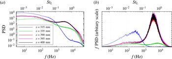
As shown in figure 3(a), the unsteadiness is broadband, without a single predominant peak. All sensors display high power spectral density (PSD) in the low-frequency range, regardless of their location. Then, depending on the distance from the shock-foot, the spectra can present a medium-frequency bump, with a PSD one order of magnitude lower than the one in the low-frequency zone. The high-frequency content due to the turbulent structures in the boundary layer probably occurs at frequencies higher than 50 kHz, not measured because of the bandwidth of the sensors (around 20 kHz).
Figure 3(b) displays the weighted PSD, where the product between the PSD and the frequency
 $f$
is shown as a function of the frequency logarithm. This representation, called premultiplied spectrum, gives access to the frequency content of the energy fluctuations. The area below this curve corresponds to the total fluctuating energy. The sensor at the shock foot reveals that most of the energy is in the low-frequency range, whilst the one in the separated zone indicate that medium-frequency motions are the most energetic.
The top horizontal axis of all figures presents the Strouhal number, obtained with a characteristic length
 $L=35$
mm, corresponding to the distance between the separation point and the impingement location of the lambda shock on the wall, and a velocity of
 $U=300~\text{m}~\text{s}^{-1}$
, corresponding to the flow speed above the recirculation bubble. This scaling yields, for the sensor placed at the shock foot, a maximum
 $f\cdot \text{PSD}$
around 0.04, which corresponds to a frequency of 300 Hz.
Wall-pressure fluctuations on the centreline of the test section. (a) Power spectral density; (b) premultiplied spectrum.

The line corresponding to
 $x=335$
mm in figure 3 illustrates that the spectrum of a pressure transducer placed close to the shock and after separation exhibits the low-frequency unsteadiness due to the shock, but also the medium-frequency due to the mixing layer. This indicates that the sensor was in an intermediary zone midway between the two phenomena. The last three sensors, placed close to the end of the separation bubble, display a very similar spectrum, indicating that pressure fluctuations inside the recirculation zone propagate downstream without changing their frequency content.
The most energetic perturbations in this zone are around 4000 Hz (
 $St_{L}=0.5$
). The scale in the premultiplied spectrum of figure 3(b) is arbitrary, but the whole spectrum is known up to a multiplicative constant, which is the same for all frequencies: the fact that the peak in the medium-frequency motions is more energetic than the low-frequency one suggests that shock motions contribute less to the total amount of unsteadiness. However, even if less energetic, low-frequency motions are present in the whole interaction, as indicated by figure 3(a), where the low-frequency spectral density is high for all the sensors. Thus, even if the weighted PSD in figure 3(b) displays a peak in the low-frequency range only at the shock foot, one can find low-frequency fluctuations also in the separated zone. On the contrary, the PSD distribution at the separation point reveals that the shock foot is only affected by low-frequency motions, with a maximum located at the zero-frequency. The frequency distribution is close to a low-pass filter, with a cutoff frequency around
 $f=300{-}400$
Hz, which corresponds to the peak of the weighted PSD in figure 3(b).
2.1.2. Skin-friction fluctuations
The purpose of this section is to present frequency spectra of skin-friction fluctuations. We used hot-film sensors, based on a thin metal film deposited on an electrically insulating substrate. Three sensors were located after the end of the bump (figure 2): one inside the recirculating bubble (
 $x=360$
mm), one around the end of the separated region (
 $x=390$
mm) and one downstream of it (
 $x=420$
mm).
The sensors (glue-on probe model 55-R47) consist of a
 $0.1\times 0.9$
mm nickel film deposited on a 0.05 mm thick polyamide foil carrying a
 $0.5~{\rm\mu}\text{m}$
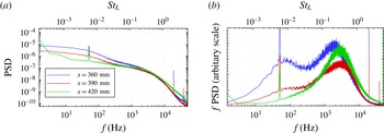
quartz coating, and were operated with a constant temperature circuit (model DISA 55M10). The signals were amplified, digitised and processed as previously described. Figure 4 presents the classic and weighted spectra: in all cases the spectrum displays a high level of PSD in the low-frequency region, and a bump at medium-frequencies. In the weighted PSD, the bump is represented by a broadband peak centred around
 $St_{L}=0.03$
, at slightly smaller frequency than in the wall-pressure fluctuations.
When a sensor is placed inside the recirculation zone and close to the shock foot (solid line corresponding to
 $x=360$
mm in figure 4) both low- and medium-frequency motions are clearly visible: the premultiplied spectrum presents a bump in the low-frequency range whose energy content is analogous to the one of the medium-frequency bump. This low-frequency content is still visible when the sensor is at the end of the recirculation zone (
 $x=390$
mm), and disappears completely for the hot-film sensor in the most downstream position (
 $x=420$
mm). The peak corresponding to
 $f=50$
Hz identified in all curves of figure 4 is a consequence of the commercial electric power distribution system and is not linked to any physical phenomenon.
Skin-friction fluctuations on the centreline of the test section. (a) Power spectral density; (b) premultiplied spectrum.

The frequency content of the low-frequency fluctuations seems however not the same when analysed with hot-films or with unsteady pressure sensors: the weighted PSD presents a maximum value at
 $f=70{-}100$
Hz when computed with hot-films signals, whilst the peak was around
 $f=300{-}400$
Hz for the Kulite sensors. We do not have a clear explanation of this discrepancy, except the fact that the two sensors have different spatial integration because of their size (the hot-film surface area is greater than those of a Kulite). Note however that if we compare hot-film and pressure curves obtained at the same location (here at the end of the recirculation zone
 $x=390$
mm), then the skin-friction and pressure spectra are close: the medium-frequency peak is located at
 $f=4$
kHz in the premultiplied pressure spectrum, while it is located at
 $f=3$
kHz in the skin-friction spectrum.
Despite the small difference in the peak location, both measurement techniques confirm the presence of low-frequency motions, mostly located at the shock foot but also in the separated region, and medium-frequency motions, localised after the separation point and not limited to the recirculation zone. This observation compares favourably with all the SWBLI studies discussed in the literature. By scaling the frequency with appropriate length and velocity scales, we obtain satisfactory agreement with results obtained in other configurations, such as compression ramps (Dolling & Brusniak Reference Dolling and Brusniak1989; Wu & Martin Reference Wu and Martin2008) or a shock impinging on a turbulent boundary layer (Dupont et al. Reference Dupont, Haddad and Debiève2006).
2.2. High-speed Schlieren visualisation
Pressure and skin-friction measurements, although very reliable, are only at few points and located at the wall. In order to have a global description of the unsteady behaviour of the interaction, we consider high-speed Schlieren visualisation. If Kulite and hot-film measurements are too local, Schlieren visualisation may suffer the opposite problem; the image obtained corresponds to a spanwise integration of the light beam, and may include three-dimensional effects due to the lateral boundary layers on the wind-tunnel walls.
Schlieren visualisation is a technique based on light deflection by a refractive index whose level is related to the flow density gradient. The deflected light beam is compared to the undeflected one by blocking the undisturbed light with a knife edge. A shadow pattern is then produced, representing the expansions and compressions in the flow. The magnitude of the density gradient is proportional to the light intensity measured by the camera sensor; a dark point on the image corresponds to negative density gradient whilst a bright point implies the presence of a positive one.
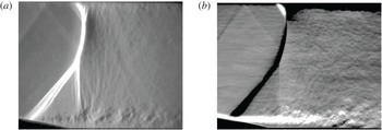
Horizontal and vertical density gradients obtained with the Schlieren apparatus. (a)
 $\partial {\it\rho}/\partial x$
: vertically-oriented knife edge; (b)
 $\partial {\it\rho}/\partial y$
: horizontally-oriented knife edge.

A high speed camera (Vision Research Phantom V710) with a
 $7~\text{Gpx}~\text{s}^{-1}$
throughput and 300 ns digital exposure is placed on the side of the wind tunnel, and 60 000 images (
 $464\times 360$
pixels) are recorded at 35 kHz frame rate. The magnification ratio is around
 $3.3~\text{px}~\text{mm}^{-1}$
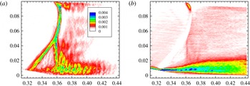
, producing an image 140 mm wide which spans the whole channel height. Both horizontal and vertical knife-edge are considered: the light intensity is proportional, respectively, to the vertical and horizontal components of the density gradient (figure 5).
Figure 5(a) presents the horizontal density gradient; the shock wave has a positive gradient and is therefore white. The boundary layers are not visible, as they are not identified by any gradient in the streamwise direction. In the instantaneous Schlieren image, the mixing layer downstream the shock foot presents a succession of positive and negative density gradients, due to the vortices shed from the separation point. Here, small and medium scale structures are responsible for the high- and medium-frequency unsteadiness. Figure 5(a) also indicates that the mixing layer is a source of noise, generating acoustic waves under the form of almost vertical Mach lines which perturb the shock.
Figure 5(b) has been obtained with a horizontal edge-oriented knife. The boundary layers exhibit wall-normal density gradients due to the fact that the flow temperature is warmest near the walls and that the wall-normal pressure gradient is zero in these regions. Hence the picture is bright on the lower wall and dark on the upper one, corresponding to positive and negative
 $\partial {\it\rho}/\partial y$
, respectively. The mixing layer on the lower-wall is bright since it is generated from the attached lower boundary layer, which was also bright. Across the shock wave, the density gradient is positive in the flow direction. The bump curvature yields a vertical velocity component which is negative, and thus the density gradient is negative.
Schlieren photography is now used to investigate the spatial structure of unsteadiness at low- and medium-frequencies. For this, we perform a Fourier-mode decomposition of the images and investigate the two-point correlations of the density gradient. The camera was equipped with a 12-bit colour depth sensor: the light intensity measured by each pixel is associated to a number between 0 and 4095. The available range is too small to describe at the same time the shock density gradient and the small variations in the mixing layer caused by the vortex shedding. For this reason, the images often exhibit colour saturation. Examples can be found in figure 5(b) on the shock (black region caused by the absence of light) or at the beginning of the mixing layer (white region associated to too much light intensity). This problem can cause signal truncation, adding high-frequency energy to the Fourier mode in the saturated zone, or showing 100 % correlation because of the absence of texture in the images.
2.2.1. Fourier-mode decomposition
In image processing, the time resolved image sequence can be written as
 $I(i,j,n)$
where
 $I$
is the light intensity of each pixel. In this study,
 $i$
and
 $j$
vary from 1 to 464 and 1 to 360,
 $n$
is the snapshot number (from 1 to
 $N=60\,000$
). The sampling frequency is 35 kHz. The time series describing the light intensity evolution at a given pixel
 $(i,j)$
can be written as
 $I_{ij}(n)$
. Assuming a linear correspondence between light intensity and density gradient, we compute the Fourier transform of
 $I_{ij}(n)$
using a FFT algorithm with a Hanning window function and 60 blocks with 50 % overlap of 2048 images.
Fourier mode at
 $f=300$
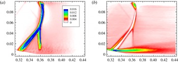
Hz for the horizontal and vertical density gradients. (a) Horizontal density gradient
 $\partial {\it\rho}/\partial x$
; (b) vertical density gradient
 $\partial {\it\rho}/\partial y$
.

Because of the reduced amount of data, the spectrum has a resolution of
 $f=17$
Hz and the blocks are insufficient to converge the statistics of the lowest frequencies. The computed frequency spectrum is noisy and may not be compared to the frequency spectra presented in § 2.1, where we used 500 blocks. Yet, relying on the informations obtained in the previous section, we consider in the following the spatial structures of a low- and a medium-frequency Fourier mode, corresponding to the peaks displayed in the premultiplied pressure spectrum of figure 3(b).
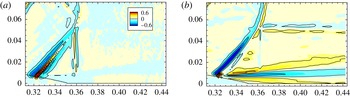
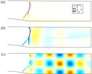
Figure 6 shows the spatial structure of the low-frequency Fourier mode at
 $f=300$
Hz. In figure 6(a) the fluctuations are located on the whole shock wave, without small scale structures after the separation point. Figure 6(b), which presents the vertical density gradient, shows that this Fourier mode has its maximum strength at the shock foot (also in the upper wall), even though the mode is located on the entire shock. The low-frequency mode is energetic also in the core of the mixing layer, where the PIV investigation of Sartor et al. (Reference Sartor, Losfeld and Bur2012) has indicated that the turbulence production has its maximal value. The absence of energy inside the shock is a consequence of the lack of light in the Schlieren images and should not be interpreted as a stationary flow region.
In the upper left side of figure 6(a) and (b) two oblique lines reveal the presence of a compression wave, generated at the sonic throat and propagating across the flow at Mach angle
 ${\it\alpha}=\sin ^{-1}(1/Ma)$
. As it will be shown in the global stability analysis, those compression waves play an important role in the flow dynamics since they indicate the directions along which informations propagate in the supersonic zone.
Figure 7 displays the Fourier mode at
 $f=4000$
Hz, located in the mixing layer region downstream of the separation point. Figure 7(a) also indicates the presence of small scale structures above the bump in the mixing layer (similar structures are also visible near the upper wall). In the shock region, the energy distribution is similar to the one in the low-frequency mode, but the energy levels are four times smaller than in the case of figure 6. Although similar features have been observed in the DNS simulations of Wu & Martin (Reference Wu and Martin2008), who documented the presence of small-amplitude spanwise wrinkling on the shock, it is believed that in the present case the medium-frequency energy comes from the truncated signal due to colour saturation.
Fourier mode at
 $f=4000$
Hz for the horizontal and vertical density gradients. (a) Horizontal density gradient
 $\partial {\it\rho}/\partial x$
; (b) vertical density gradient
 $\partial {\it\rho}/\partial y$
.

The medium-frequency mode in figure 7(b) suggests that the most energetic fluctuations are in the mixing layer, whilst the shock does not present any medium-frequency unsteadiness. This result confirms that medium-frequency motions on the shock are spurious, and only the mixing layer is affected by those motions.
Although less detailed in frequencies, the Fourier-mode decomposition confirms the presence of two characteristic modes. Medium-frequency perturbations are mainly located in the mixing layer. Using LES flow fields, Pirozzoli et al. (Reference Pirozzoli, Larsson, Nichols, Bernardini, Morgan and Lele2010) performed a Fourier analysis and found similar results in a shock-impinging configuration. We also found that low-frequency perturbations are not only restricted to the shock foot, but affect the whole shock wave and even the top of the recirculation bubble. The mixing layer has therefore energetic contributions in both the low- and medium-frequency Fourier modes. A similar result has recently been observed in a compression ramp configuration (Grilli et al. Reference Grilli, Schmid, Hickel and Adams2012), where a dynamic mode decomposition (Schmid Reference Schmid2010) documented the presence of a low-frequency mode associated to the pulsation of the separation bubble and accompanied by a forward–backward shock motion.
2.2.2. Two-point correlations
In this section, a set of
 $N=20\,000$
images is employed for analysing two-point correlations, which can give insights on the coherent structures of the flow, regardless of the frequency. As before, the light intensity of a given pixel at time
 $n$
can be written as
 $I_{ij}(n)$
. If we consider another pixel on the image, with coordinates
 $(k,l)$
, one can compute the correlation between the time series at point
 $(k,l)$
, indicated as
 $I_{kl}(n)$
, and the time series at all other points
 $I_{ij}(n)$
. When processing images where the brightness varies from image to image due to lighting, it is recommended to first subtract the mean and then normalise the results by dividing by the standard deviation of each data sequence. The cross-correlation coefficient is then given by:
 $$\begin{eqnarray}C_{kl}(i,j)=\frac{1}{N}\mathop{\sum }_{n=1}^{N}\frac{[I_{ij}(n)-\overline{I_{ij}}][I_{kl}(n)-\overline{I_{kl}}]}{{\it\sigma}_{ij}{\it\sigma}_{kl}},\end{eqnarray}$$
where
 $\overline{I_{ij}}$
is the mean value of the light intensity and
 ${\it\sigma}_{ij}$
and
 ${\it\sigma}_{kl}$
are the standard deviations. The result of this operation is a set of
 $464\times 360$
fields which represent, for each interrogation point
 $(k,l)$
, the correlation between the chosen pixel and the whole image. The approach proposed in this section consists in fixing an interrogation point, for example at the shock foot or in the mixing layer, and investigating the zones of the flow where the density gradients are correlated to that point. Contrary to the correlation analyses based on wall-pressure measurements (Dolling & Erengil Reference Dolling and Erengil1991; Dupont et al.
Reference Dupont, Haddad and Debiève2006) or on numerical simulation data (Larchevêque et al.
Reference Larchevêque, Dupont, De Martel, Garnier and Debiève2010; Touber & Sandham Reference Touber and Sandham2008), the correlations computed here are based on light intensity.
Correlations when the reference point (
 $+$
symbol) is at the shock foot. (a) Horizontal density gradient
 $\partial {\it\rho}/\partial x$
; (b) vertical density gradient
 $\partial {\it\rho}/\partial y$
.

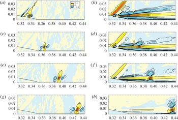
Figure 8 presents the correlation maps when the reference point is at the shock foot. A strong correlation exists with the whole shock wave, suggesting that shock movements are rigid-body displacements. The horizontally elongated correlated regions observed in the mixing layer of figure 8(b) reveal that the shock movements are linked to vertical displacements of the separated zone: due to the bump slope, shock movements correspond to vertical displacements of the separation point, which induce contractions and expansions of the recirculation bubble. This result has already been observed by Kussoy et al. (Reference Kussoy, Brown, Brown, Lockman, Horstman, Hirata and Kasagi1988) in flow past a flared cylinder.
Correlations when the reference point (
 $+$
symbol) is in the mixing layer. (a) Horizontal density gradient
 $\partial {\it\rho}/\partial x$
; (b) vertical density gradient
 $\partial {\it\rho}/\partial y$
.

We have also found that the boundary layer fluctuations are not correlated to the shock or the mixing layer fluctuations, even if this observation is limited by the spatial resolution of the Schlieren pictures. On the contrary, when considering a point in the mixing layer, the spatial resolution of the Schlieren images is sufficiently fine to identify vortices generated near the separation point, as in figure 9. For example, when considering the horizontal density gradient, the correlation maps reveal the presence of large scale structures which can be linked to vortex shedding.
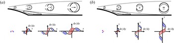
The sketch in figure 10(a) helps understanding of the horizontal density gradient distribution generated by three downstream travelling co-rotating vortical structures; on the lower part of the image, the density gradient is represented for two realisations. The correlation map highlights the region in the mixing layer with similar density gradient distributions, due to the passage of vortical structures. The result is a positive correlation on the reference point (red arrows) in the mixing layer, surrounded by two negatively correlated regions upstream and downstream of this point (blue arrows). A similar behaviour can be observed in figure 10(b) with the negatively correlated regions above and below the correlation point. The distance between the positive and negative correlation regions indicates the characteristic size of the shed vortices, which evolve spatially as moving downstream.
Density gradient distribution when vortical structures are shed in the mixing layer. (a) Horizontal density gradient
 $\partial {\it\rho}/\partial x$
; (b) vertical density gradient
 $\partial {\it\rho}/\partial y$
.

When considering the vertical density gradient correlations (figure 9 b), the relation between the mixing layer movements and the shock displacements is even more evident; close to the separation, the shock foot and the mixing layer are highly correlated. In this region, the Fourier-mode decomposition showed high energy at low frequencies. Considering reference points more downstream in the mixing layer, the shock movements become less correlated, while vortical structures begin to appear. These structures are generated by Kelvin–Helmholtz type instabilities linked to the inflection point of the shear layer. Similar circular periodic patterns have also been observed in a shock reflection configuration by Agostini et al. (Reference Agostini, Larchevêque, Dupont, Debiève and Dussauge2012) and associated to medium-frequency unsteadiness using band-pass filtering.
3. Numerical approach
The experimental investigations have shown that the low- and medium-frequency perturbations exhibit characteristic frequencies and spatial wavenumbers below those of the small scale motions representative of turbulence. It seems therefore reasonable that the scale-decoupling assumption holds within such a flow. Hence, the dynamics of the large scales might be captured by time-integration of RANS equations, while the impact of small scale dynamics on the large ones is accounted for by a turbulence model.
In this section, we consider a numerical model based on RANS equations closed with a Spalart–Allamaras turbulence model. First (§ 3.1) we will march in time these equations and observe that the flow converges to a steady-state solution. This indicates that unforced RANS equations are not able to capture the low- and medium-frequency perturbations. The asymptotic two-dimensional solution is then considered as a base flow for linear stability analyses. Both global modes of the Jacobian (§ 3.2) and singular modes of the Resolvent (§ 3.3) are computed.
3.1. Base flow
The simulations were performed using the finite volume solver elsA v3.3, developed at ONERA and CERFACS (Cambier, Heib & Plot Reference Cambier, Heib and Plot2013). Numerical computations were performed in parallel over up to 64 cores on ONERA’s high-performance computer Stelvio, using
 $2.8$
GHz Intel Xeon 5560 (Nehalem) processors. After spatial discretisation, the governing equations can be recast in the general conservative form:
 $$\begin{eqnarray}\frac{\text{d}\boldsymbol{w}}{\text{d}t}=\mathscr{R}(\boldsymbol{w}),\end{eqnarray}$$
where
 $\boldsymbol{w}\in \mathbb{R}^{N}$
represents the set of conservative variables describing the flow at each spatial location in the domain and
 $\mathscr{R}$
represents the discrete residual. Using a finite volume method, the dimension of
 $\boldsymbol{w}$
corresponds to the number of cells in the mesh times the number of variables. Note that all boundary conditions are included in the discrete operator
 $\mathscr{R}$
.
The Spalart–Allmaras (S–A) turbulence model (Spalart & Allmaras Reference Spalart and Allmaras1992) has been chosen because previous studies (Deck Reference Deck2005; Crouch, Garbaruk & Magidov Reference Crouch, Garbaruk and Magidov2007; Sartor et al. Reference Sartor, Mettot and Sipp2015) proved its ability to correctly reproduce the challenging buffet configuration. A second-order AUSM+(P) upwind scheme is employed for the convective fluxes in the mass, momentum and energy conservation equations (Mary, Sagaut & Deville Reference Mary, Sagaut and Deville2000). Roe and Jameson schemes were not considered due to difficulties to converge to a steady-state solution. The convective flux associated to the turbulence equation is discretised with the first-order Roe scheme with Harten’s correction (Harten & Hyman Reference Harten and Hyman1983), whilst a central-difference scheme is used for the turbulent diffusive flux.
The boundary conditions have been chosen to match the experimental configuration described in § 2; both upper and lower walls are considered as adiabatic walls and the boundary layers start developing in the settling chamber. The outlet pressure condition is adjusted to place the shock wave close to the position in the experimental configuration (approximately
 $p=62$
kPa at
 $x=0.65$
m). The computational domain, partly visible in figure 11, is a two-dimensional single-block representation of the S8Ch wind tunnel, composed of 120 000 nodes; 300 in the vertical direction, and 400 in the streamwise direction. In the shock region, the average distance between two mesh points is 0.45 mm. Considering the interaction length
 $L$
as a characteristic dimension, this corresponds to a resolution of
 ${\it\Delta}_{x}/L=0.013$
. Eighty cells have been used to discretise the wall-normal gradients in the boundary layers, while the first point is located at
 $y^{+}=0.6$
.
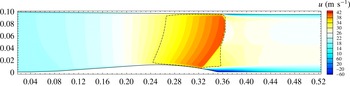
RANS simulation: steady-state solution of the wind-tunnel test section. Iso-contour of streamwise velocity and dashed-dotted sonic line.

To assess the spatial convergence of the solutions, two other meshes are considered; a coarser mesh, with
 ${\it\Delta}_{x}/L=0.020$
in the interaction region, and a finer one, with
 ${\it\Delta}_{x}/L=0.065$
. All grids converge to the same RANS solution in terms of shock location, size of the recirculation bubble and separation-point position, but the shock thickness increases with decreasing the cell size. As will be shown in the next sections, this does not impact the results of the global-mode decomposition, but slightly influences those of the singular-value.
3.1.1. Results
The resulting velocity field is displayed in figure 11, with a dashed-dotted sonic line. On the upper wall, the shock pressure gradient induces separation of the turbulent boundary layer, and a small separation bubble is formed.
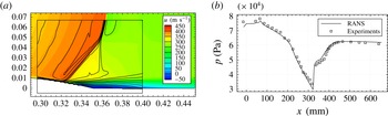
Figure 12(a) shows a comparison between the experimental time-averaged PIV measurements obtained by Sartor et al. (Reference Sartor, Losfeld and Bur2012) and those of the RANS simulation. The shock position compares favourably on the top, but in the numerical simulation the shock foot is slightly downstream. Moreover, the PIV results indicate a thicker shock, but this may come from the averaging of the shock unsteadiness in the experiments. The average pressure on the wall is depicted in figure 12(b); a rise of static pressure begins at
 $x=320$
mm, corresponding to the shock foot. The recirculation bubble is characterised by a small pressure plateau, and after the separated zone the pressure reaches the value imposed at the downstream boundary.
Comparison between the experimental results (pressure taps and PIV measurements from Sartor et al. (Reference Sartor, Losfeld and Bur2012)) and the base flow (RANS solution). (a) Velocity field; (b) wall pressure.

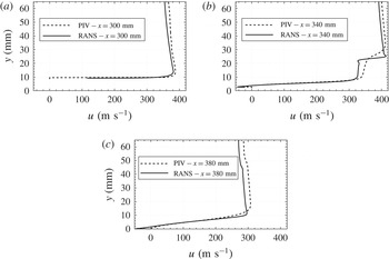
Velocity profiles from the numerical investigation and the PIV measurement. (a) Upstream of the shock; (b) in the interaction region; (c) downstream of the bubble.

Figure 13 presents three velocity profiles, taken upstream of the shock wave (
 $x=300$
mm), in the interaction region (
 $x=340$
mm) and downstream of the separated zone (
 $x=380$
mm). The PIV measurement and the RANS result are in fair agreement outside the separated region, with a slight velocity deficit in the numerical simulation (figure 13
a,c). In figure 13(b), PIV measurements indicate similar velocities inside the recirculation zone and in the supersonic region, but a different distribution across the shear layer. This discrepancy can be attributed to the different lambda shape of the shock, probably due to three-dimensional effects in the wind tunnel.
Overall, RANS computations are in a fair agreement with the experimental investigation. Note that the characteristic length and velocity scales used in the following to obtain the Strouhal number are those of the experimental investigation.
Unsteady RANS simulations with a time step of
 ${\rm\Delta}t=10^{-6}$
s (corresponding to a maximum CFL number of 20) indicate a stationary solution. The velocity field obtained is the same as the steady-state result obtained with a local time stepping. This is not surprising since Knight & Degrez (Reference Knight and Degrez1998) analysed the numerical capabilities of RANS approaches and stated that turbulent interaction predictions are correct only in terms of mean-pressure distribution: in this case, (unforced) RANS computations fail to predict the intermittent separation stage and to capture the high levels of unsteadiness.
As will be shown in the next section, inviscid phenomenon can have a strong signature on the results of the stability analysis. To separate the effect of the interaction with the boundary layers form the acoustic resonances, we considered a configuration with an equivalent geometry, but with slip conditions on both upper and lower walls. A new base flow is obtained, without any boundary layers and separated regions, with a normal shock impinging on the bump. The outlet pressure was adapted to locate the shock at approximately the same position as the configuration with boundary layers. The absence of viscous effects allows for the investigation of the role of the shock in the perturbation dynamics independently from those of the separated region.
The flow is governed by (3.1). The unsteady RANS computations indicate that a steady solution
 $\boldsymbol{w}_{\mathbf{0}}\in \mathbb{R}^{N}$
exists, referred to as the base flow. This solution is defined by the equation:
 $$\begin{eqnarray}\mathscr{R}(\boldsymbol{w}_{\mathbf{0}})=\mathbf{0}.\end{eqnarray}$$
Since the governing system contains the Spalart–Allmaras equation, the base flow
 $\boldsymbol{w}_{\mathbf{0}}$
takes into account the Reynolds stresses involved in the turbulence model. The vector
 $\boldsymbol{w}_{\mathbf{0}}$
thus represents
 $$\begin{eqnarray}\boldsymbol{w}_{\mathbf{0}}=({\it\rho}_{0},{\it\rho}U_{0},{\it\rho}V_{0},{\it\rho}E_{0},{\it\rho}{\it\nu}_{0})^{\text{T}},\end{eqnarray}$$
where
 ${\it\rho}{\it\nu}$
is introduced by the turbulence model. The subscript 0 indicates that all the variables refer to the steady-state solution of the RANS simulation. The stability of the flow is probed by analysing the evolution of small amplitude perturbations, superimposed on the base flow, which involve variations of the turbulent quantities.
3.2. Global modes
The equation governing small-amplitude perturbations is given by the first-order linearization of the discretised equations (3.1):
 $$\begin{eqnarray}{\displaystyle \frac{\text{d}\boldsymbol{w}^{\prime }}{\text{d}t}}=\unicode[STIX]{x1D645}\boldsymbol{w}^{\prime }.\end{eqnarray}$$
The Jacobian operator
 $\unicode[STIX]{x1D645}\in \mathbb{R}^{N\times N}$
corresponds to the linearization of the discrete Navier–Stokes operator
 $\mathscr{R}$
around the base flow
 $\boldsymbol{w}_{\mathbf{0}}$
. The proposed formalism does not assume homogeneity of the base flow in a given direction, and corresponds to the BiGlobal linear-stability analysis as introduced by Theofilis (Reference Theofilis2003). The analysis is two-dimensional, and we assume that the base flow and the fluctuations are homogeneous in the third direction.
The stability of a base flow is determined by scrutinising the spectrum of the matrix
 $\unicode[STIX]{x1D645}$
. To this end, particular solutions of (3.4) are sought in the form of normal modes
 $\boldsymbol{w}^{\prime }=\hat{\boldsymbol{w}}\text{e}^{{\it\lambda}t}$
, where
 ${\it\lambda}={\it\sigma}+\text{i}{\it\omega}$
describes the temporal behaviour (
 ${\it\sigma}$
is the amplification rate and
 ${\it\omega}$
the frequency) and
 $\hat{\boldsymbol{w}}\in \mathbb{C}^{N}$
the spatial structure. Since the governing equations involve a turbulence model, the perturbation includes variations of the turbulent quantities, and the turbulence model equation is also linearised. Hence (3.4) may be recast into the following eigenvalue problem:
 $$\begin{eqnarray}\unicode[STIX]{x1D645}\hat{\boldsymbol{w}}={\it\lambda}\hat{\boldsymbol{w}}.\end{eqnarray}$$
If at least one of the eigenvalues
 ${\it\lambda}$
exhibits a positive growth rate
 ${\it\sigma}$
, the base flow
 $\boldsymbol{w}_{\mathbf{0}}$
is unstable. To compute the linearised operator, we follow a strategy based on a finite difference method, introduced by Mettot et al. (Reference Mettot, Renac and Sipp2014a
), where the Jacobian coefficients are computed by repeated residual evaluations provided by the numerical code. More details on the numerical strategy can be found in Mettot et al. (Reference Mettot, Renac and Sipp2014a
), Sartor et al. (Reference Sartor, Mettot and Sipp2015) or Beneddine, Mettot & Sipp (Reference Beneddine, Mettot and Sipp2015), who successfully applied this method to open-cavity flow, transonic buffet and under-expanded screeching jets.
3.2.1. Results
To ease comparison with the experimental investigation, the results will be discussed using the dimensional frequency
 $f$
(expressed in Hertz) and the Strouhal number
 $St_{L}$
instead of the pulsation
 ${\it\omega}$
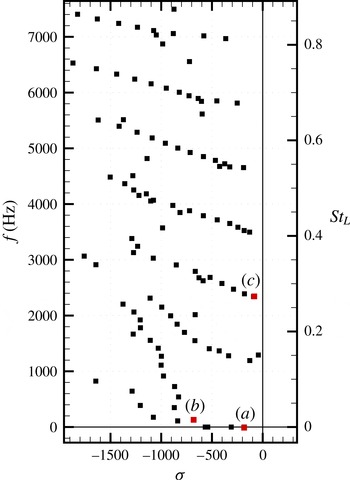
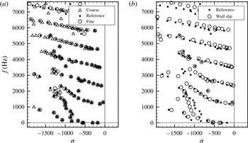
. The spectrum and the global modes, depicted in figures 14 and 15, are obtained by computing the five closest eigenvalues with respect to a given shift. Among the eigenvalues, which are all damped since they display a negative real part, one can recognise a group of modes in the lower part of the spectrum in the range of Strouhal numbers corresponding to the low-frequency unsteadiness.
Spectrum.

Stable global modes. (a) Real part of the stable mode at
 $f=0$
Hz; (b) real part of the stable mode at
 $f=130$
Hz; (c) real part of the stable mode at
 $f=2340$
Hz.

Figure 15 shows the real part of some of those modes. The first (figure 15 a) is located on the shock wave and represents a global movement of the shock structure. Yet, since the mode is stationary, it does not carry any information about the unsteady behaviour of the interaction. Similarly, the second one (figure 15 b) is also located on the shock, but with the addition of the slip line and a weak large scale streamwise oscillation in the subsonic region. Such a structure could correspond to an acoustic wave that resonates with the test section, and which triggers solid-body movements of the shock wave.
Considering higher Strouhal numbers, one can recognise that the eigenvalues in figure 14 are grouped in periodic quasi-horizontal line, with some scattering when the damping rate becomes strong. The spatial structure of the least damped mode on one of those lines is presented in figure 15(c); the shock wave is still visible, but the horizontal and vertical wavy structures suggest that the mode is probably acoustic. Those structures propagate upstream preserving their shape while travelling towards the shock wave. All the stable modes just discussed are probably not linked to the unsteady dynamics of the SWBLI, but rather to some acoustic resonance of the channel flow.
In this configuration, as for a generic flow in a duct, if the acoustic wavelength has the same size as the device, the acoustic standing wave resonances may dominate the flow (Koch Reference Koch2005). The spatiotemporal structure of the mode actually reveals that all the modes correspond to acoustic resonance modes linked to the channel height. All the modes belonging to the same periodic quasi-horizontal line are characterised by the same number of zeros in the vertical direction; one zero for the group characterised by
 $f\approx 1200$
Hz, two zeros for the group of eigenvalues such that
 $f\approx 2400$
Hz, etc. Regarding the size of the structures in the streamwise direction, we have verified that the streamwise wavelength
 $L$
is related to the frequency
 $f$
and the upstream travelling velocity of acoustic waves
 $|u-a|$
through
 $L=|u-a|/f$
, where
 $u$
is the local flow speed.
None of the analysed global modes in the medium-frequency range (more than 100 modes have been scrutinised) exhibit a spatial structure that can be linked to mixing layer instabilities, as would have been expected from the experimental investigation. We believe that such modes exist, but that they are even more damped. This suggests that in some cases the global mode decomposition is not the most convenient approach to explore medium-frequency perturbations in a transonic channel flow.
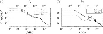
As previously introduced, a coarser and a finer mesh have been considered to assess grid convergence. Figure 16(a) shows the superposition of the spectra obtained with different meshes; nearly all the eigenvalues are converged, especially for low frequencies. Some discrepancies appear at higher frequencies, consistent with the fact that these modes are associated to small scale structures, and coarser meshes can cause spatial filtering. However, the frequencies associated to those structures are outside the range of interest of the study, so the reference grid can be considered adapted for the purpose of the investigation. Figure 16(b) presents the comparison between the eigenvalues of the reference case and those obtained when considering a base flow with slip conditions (see § 3.1). The absence of boundary layers and recirculation bubble barely influences the spectrum; the eigenvalues are still grouped into quasi-horizontal lines, confirming that these modes represent acoustic resonances and not the interaction dynamics. Low-frequency eigenvalues are slightly more damped, and no high-frequency modes appear or disappear from the reference spectrum.
Eigenvalue decomposition of the Jacobian matrix. (a) Grid convergence; (b) effect of boundary layers.

3.3. Singular modes
If all the global modes are stable, the interaction behave as a noise amplifier. In this case, the transient energy growth is intrinsically linked to the non-normality of the Jacobian matrix (Trefethen et al.
Reference Trefethen, Trefethen, Reddy and Driscoll1993; Schmid Reference Schmid2007) and an external driving term is now required to sustain the perturbations. This term stands for the environmental disturbance, which is naturally present in any real flow. The stability analysis aims at quantifying the input/output dynamics by identifying the pseudo-resonances of the interaction. We therefore consider the response of the flow to a small-amplitude forcing
 $\boldsymbol{f}^{\prime }$
:
 $$\begin{eqnarray}\frac{\text{d}\boldsymbol{w}}{\text{d}t}=\mathscr{R}(\boldsymbol{w})+\boldsymbol{f}^{\prime },\end{eqnarray}$$
 $\boldsymbol{w}$
is the superposition of the base flow
 $\boldsymbol{w}_{\mathbf{0}}$
plus a small-amplitude response
 $\boldsymbol{w}^{\prime }$
and is driven by the external forcing
 $\boldsymbol{f}^{\prime }$
. Considering a first-order Taylor expansion of the residual, the response
 $\boldsymbol{w}^{\prime }$
is governed by the forced linearised Navier–Stokes equations. We consider a harmonic forcing
 $\boldsymbol{f}^{\prime }(x,y,t)$
at frequency
 ${\it\omega}$
and a harmonic response
 $\boldsymbol{w}^{\prime }(x,y,t)$
in the form
 $\boldsymbol{f}^{\prime }=\hat{\boldsymbol{f}}(x,y)\text{e}^{\text{i}{\it\omega}t}$
and
 $\boldsymbol{w}^{\prime }=\hat{\boldsymbol{w}}(x,y)\text{e}^{\text{i}{\it\omega}t}$
, with
 $\hat{\boldsymbol{f}},\hat{\boldsymbol{w}}\in \mathbb{C}^{N}$
. Simplifying and re-arranging the equation for
 $\hat{\boldsymbol{w}}$
yields:
 $$\begin{eqnarray}\hat{\boldsymbol{w}}=\unicode[STIX]{x1D64D}\hat{\boldsymbol{f}},\end{eqnarray}$$
where
 $\unicode[STIX]{x1D64D}({\it\omega})$
is the global resolvent matrix
 $\unicode[STIX]{x1D64D}=(\text{i}{\it\omega}\unicode[STIX]{x1D644}-\unicode[STIX]{x1D645})^{-1}$
and
 $\unicode[STIX]{x1D644}$
is the identity.
The resolvent matrix
 $\unicode[STIX]{x1D64D}({\it\omega})$
is defined for any real forcing frequency
 ${\it\omega}$
since all eigenvalues of
 $\unicode[STIX]{x1D645}$
are strictly damped. The relation in (3.7) gives access, for a given frequency, to the harmonic response of the system when forced with a harmonic forcing of a given spatial form. We now introduce the gain
 $G$
, function of the external forcing
 $\hat{\boldsymbol{f}}$
and defined for every frequency, as the ratio between the energy of the response and the energy of the forcing itself:
 $$\begin{eqnarray}G(\hat{\boldsymbol{f}})=\frac{\langle \hat{\boldsymbol{w}},\hat{\boldsymbol{w}}\rangle _{\boldsymbol{Q}_{\boldsymbol{e}}}}{\langle \,\hat{\boldsymbol{f}},\hat{\boldsymbol{f}}\rangle _{\boldsymbol{Q}_{\boldsymbol{f}}}},\end{eqnarray}$$
where
 $\langle \cdot ,\cdot \rangle _{\boldsymbol{Q}_{\boldsymbol{e}}}$
and
 $\langle \cdot ,\cdot \rangle _{\boldsymbol{Q}_{\boldsymbol{f}}}$
respectively refer to the scalar products that quantify the strength of the response and of the forcing. Here we chose the kinetic energy of the perturbation for the response
 $\hat{\boldsymbol{w}}$
and the energy of the momentum forcing for
 $\hat{\boldsymbol{f}}$
.
Among all the possible forcings, we are looking for the one that causes the strongest gain
 $G$
, called the optimal forcing. Inserting (3.7) into (3.8) yields, for each frequency
 ${\it\omega}$
, an optimisation problem that can be solved through a singular-value decomposition of the global resolvent
 $\unicode[STIX]{x1D64D}({\it\omega})$
, which may also be written as:
 $$\begin{eqnarray}\unicode[STIX]{x1D64D}^{\dagger }\unicode[STIX]{x1D64D}\hat{\boldsymbol{f}}={\it\lambda}^{2}\hat{\boldsymbol{f}}.\end{eqnarray}$$
where
 $\unicode[STIX]{x1D64D}^{\dagger }$
is the operator adjoint to
 $\unicode[STIX]{x1D64D}$
. The real eigenvalue
 ${\it\lambda}^{2}$
is related to the forcing
 $\hat{\boldsymbol{f}}$
, which we choose of unit norm
 $\langle \hat{\boldsymbol{f}},\hat{\boldsymbol{f}}\rangle _{\boldsymbol{Q}_{\boldsymbol{f}}}=1$
. The largest eigenvalue of this eigenproblem is
 ${\it\lambda}_{max}^{2}$
, which corresponds to the optimal gain
 $G$
. Once the corresponding optimal forcing is computed, the associated optimal response
 $\hat{\boldsymbol{w}}$
can be obtained solving (3.7) and verifies
 $\langle \hat{\boldsymbol{w}},\hat{\boldsymbol{w}}\rangle _{\boldsymbol{Q}_{\boldsymbol{e}}}={\it\lambda}_{max}^{2}$
. For more details and an application of this approach the reader is referred to Sipp & Marquet (Reference Sipp and Marquet2013) and Sartor et al. (Reference Sartor, Mettot and Sipp2015).
3.3.1. Results
The singular values
 ${\it\lambda}^{2}$
have been non-dimensionalised with the reference length, velocity and density scales (
 $L=35$
mm,
 $U=300~\text{m}~\text{s}^{-1}$
and
 ${\it\rho}=0.73$
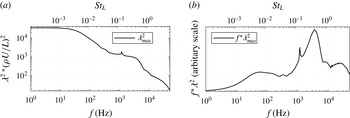
). Note that the value one does not define a threshold between damping and amplification; the role of the gain curve is to determine if there exist preferred frequencies in a flow excited by broadband white noise forcing. The optimal gain
 ${\it\lambda}^{2}({\it\rho}U/L)^{2}$
has been represented as a function of frequency in figure 17. We observe that the strongest flow responses are obtained for low frequencies up to 50 Hz; then the gain decreases rapidly and reaches a plateau for frequencies within 1–4 kHz. This curve strongly resembles the experimental PSD curves obtained when processing pressure (figure 3
a) and skin-friction measurements (figure 4
a). For example, we both recover the strong flow response at low frequencies and the weaker plateau at medium frequencies.
Most energetic singular value of the global resolvent. (a) Gain function, logarithmic scale; (b) normalised premultiplied optimal gain.

The weighted gain
 $f{\it\lambda}^{2}$
has been represented in figure 17(b) as a function of frequency. This curve closely resembles the weighted PSD curves presented in figures 3(b) and 4(b). It displays a peak near
 $f=50$
Hz, indicating the frequency where the energy content of the flow response is maximal. This peak occurs approximately at the same frequency as the one obtained with the hot-film sensors (figure 4
b). Concerning the medium-frequency unsteadiness, the experimental measurements predicted a peak in pressure and skin-friction unsteadiness around
 $f=2{-}5$
kHz (figures 3 and 4), in good agreement with the value of
 $f=3{-}4$
kHz of figure 17(b). In spite of this, the reader should keep in mind that the results of the experimental investigation are issued from local measurements, while the gain function is a global quantity.
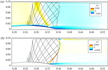
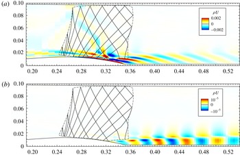
The optimal forcing obtained at the low frequency
 $f=50$
Hz is shown in figure 18(a); it is located mostly in the boundary layer on the divergent part of the bump and is strongest at the shock foot. Starting from the top of the bump, the optimal forcing forms an oblique pattern that bounces on the upper sonic line and then hits the shock foot. To investigate the nature of this line we consider the theory of characteristics (Délery Reference Délery2010). The oblique part of the forcing in figure 18(a) follows exactly the right characteristic line that impacts on the shock foot, where the recirculation bubble begins; the separation point therefore has a fundamental importance in the dynamics of the flow, and forcing at this position optimally influences the low-frequency dynamics. As the information propagates along the characteristic lines, the optimal forcing is energetic on the lines along which information propagates and impacts the separation point. More details can be found in Sartor et al. (Reference Sartor, Mettot and Sipp2015), where a similar structure has been found in the case of a transonic flow over aerofoils, and has been observed in the adjoint unstable global mode associated to transonic buffet.
Real part of the optimal forcing and associated response at
 $f=50$
Hz. Sonic line (dash-dotted) and characteristics (solid) superimposed. (a) Optimal forcing; (b) optimal response.

The optimal response associated to the low-frequency forcing is presented in figure 18 b: the mode is located mostly on the shock wave, with a spatial form similar to what has been observed for the low-frequency Fourier mode of figure 6. Part of the response is located in the core of the mixing layer, with a horizontal structure of large wavelength. The presence of a negative value of the mode in the mixing layer, associated to a positive value on the shock, implies that the contraction of the bubble is related to a downstream motion of the reflected shock, whereas its expansion is related to intense reverse flow and, consequently, upstream motion of the reflected shock. This observation is consistent with the model proposed by Piponniau et al. (Reference Piponniau, Dussauge, Debiève and Dupont2009).
Real part of the optimal forcing and associated response at
 $f=4000$
Hz. Sonic line (dash-dotted) and characteristics (solid) superimposed. (a) Optimal forcing; (b) optimal response.

The medium-frequency optimal forcing at
 $f=4$
kHz and its induced response are shown in figure 19. The spatial structure of the forcing is now more elaborated. It is still located both in the supersonic and subsonic regions, with strong values at the shock foot and at the beginning of the mixing layer. Yet, it is not anymore located along the characteristic lines. Similarly to the results of Marquet et al. (Reference Marquet, Sipp, Chomaz and Jacquin2008), we observe forcing structures which lay against the shear, confirming that the Orr (Orr Reference Orr1907) mechanism is at play here. The medium-frequency forcing induces a response which is not localised on the shock-wave inside and along the mixing layer. Note that no acoustic wave pattern can be seen in the channel, indicating that this mode couples only weakly with acoustic waves. The present picture reminds the medium-frequency Fourier mode presented in figure 7. Finally, we observe medium scale wavelength structures due to Kelvin–Helmholtz type (Drazin & Reid Reference Drazin and Reid1980) instabilities, indicating that the medium-frequency unsteadiness is associated to vortex shedding.
To describe those motions, a Strouhal number based on the local mixing layer thickness
 ${\it\delta}_{{\it\omega}}(x)$
, rather than on the interaction length
 $L$
, is probably more significant. This quantity can be evaluated using the PIV measurement or the RANS result, and its value in a streamwise location corresponding to the centre of the separated zone (
 $x=355$
mm) is
 ${\it\delta}_{{\it\omega}}=6$
mm. The most appropriate velocity to compute the Strouhal number for Kelvin–Helmholtz instability is the mixing layer average speed, given by
 ${\rm\Delta}U=(U_{1}-U_{2})/2=180~\text{m}~\text{s}^{-1}$
, where
 $U_{1}$
and
 $U_{2}$
are the flow velocities outside the mixing layer. This scaling would yield
 $S_{{\it\delta}}=0.13$
for the medium-frequency unsteadiness, instead of
 $St_{L}=0.5$
when using the interaction length and the reference velocity.
Grid convergence is assessed in figure 20(a). It is shown that medium- and high-frequency motions are well converged, while at low frequencies the gain is more energetic for a finer grid. This is not surprising since in this case the response of the flow is located on the shock, while we know that a finer grid has a strong impact on the representation of the shock wave (see § 3.1). We believe that even finer grids are required to converge the optimal gain curve at low frequencies. Yet, the main features presented here should remain unchanged.
Optimal gain as a function of frequency. (a) Grid convergence; (b) effect of boundary layers.

Isolated peaks, located around
 $f=1200$
Hz and its multiples, are visible in the gain function. To investigate their nature, we consider again the wall-slip configuration introduced in § 3.1. The new gain function (figure 20
b) presents isolated peaks at the above mentioned frequencies. The associated responses are shown to be similar to the mode presented in figure 15(c). This indicates that these peaks are linked to acoustic resonance phenomena. Also, these peaks reflect the presence of weakly damped global modes in the spectrum shown in figure 16. Without boundary layers and recirculation region, it is seen that the evolution of the optimal gain still reveals a higher gain at low frequencies than at medium frequencies. Hence, even in this simplified case, the shock should react preferentially to low-frequency motions.
4. Conclusions
The main purpose of this study was twofold: to describe experimentally the unsteady dynamics of the transonic interaction between a strong shock and a turbulent boundary layer developing over the Délery bump; and to address the problem of unsteadiness in SWBLI employing stability analyses.
In the experimental investigation, wall-pressure and skin-friction fluctuations gave access to a local description of the unsteadiness. Near the shock foot, the low frequencies dominate the spectrum, while after the separation point medium-frequency fluctuations are most energetic. The recirculation zone displays both low- and medium-frequency unsteadiness. Similarly to other SWBLI, the fluctuations are broadband and weak in amplitude. The Strouhal numbers representative of low- and medium-frequency unsteadiness compare favourably with other configurations. An innovative investigation using high-speed Schlieren photography allowed for a more complete characterisation of the interaction: Fourier-mode decomposition indicated where low- and medium-frequency unsteadiness are most energetic. The results confirm the separation of temporal scales between the unsteadiness in the shock and the mixing layer. Cross-correlation maps showed that shock motions undergo rigid-body displacements accompanied by expansion and contraction of the recirculation bubble. In the mixing layer region, the medium-frequency perturbations are due to Kelvin–Helmholtz instabilities, which generate vortex shedding.
The interaction has been investigated numerically. It has been shown that unsteady RANS simulations converge toward a steady-state solution, which compares favourably with the mean PIV and wall-pressure measurements. Global stability analyses have then been conducted: the RANS equations were linearised around the base flow, and the Jacobian matrix explicitly extracted. The eigenvalue decomposition indicates that the flow is globally stable for two-dimensional perturbations, and the least stable eigenvalues cannot be related to the unsteadiness. Pseudo-resonances of the flow have then been identified by computing the singular values of the global resolvent. Such an input/output approach aims at characterising the receptivity of the flow to external forcings. It has been confirmed that low-frequency unsteadiness is due to a preferred response of the flow to existing environmental noise at low frequencies. The optimal forcings are concentrated both upstream and downstream of the shock, with a strong sensitivity at the shock foot. In the supersonic region, low-frequency forcings are also located along the right characteristic lines that impinge on the separation point. Medium-frequency unsteadiness is linked to Kelvin–Helmholtz instabilities, which exist regardless of the presence of the shock wave.
From a broader perspective, the considered two-dimensional interaction has potential for transient growth. If this behaviour were typical of all SWBLI, such flows would be better characterised by analysing the singular values and vectors of the global resolvent, and not the eigenvalues of the Jacobian matrix. Regarding the origin of the unsteadiness, it has been shown that both perturbations in the incoming flow and in the recirculation bubble may trigger shock unsteadiness. If this behaviour is conserved in three-dimensional cases, the source of low-frequency motions may not be unique. The authors support the idea that the interaction responds as a dynamical system which is affected by external or internal disturbances; if forced by an external agent, the flow will respond. However, even in the absence of this forcing, low-frequency oscillations can be caused by coupling between the dynamics of the separation bubble and the shock.
Acknowledgements
The authors would like to acknowledge the financial support of the French agency ANR through the DECOMOS program (compressible separated flows and self-sustained oscillations, ANR-10-BLANC-914). This work wouldn’t have been possible without the constant guidance of Professor J.-P. Dussauge and P. Dupont, from the Supersonic Group of the IUSTI lab (Aix-Marseille Université). We are also grateful to Y. Le Sant, from ONERA – DAFE Department, for the wonderful tool that he developed for analysing and post processing the Schlieren images.