The Paradox of Voter Participation? A Laboratory Study

DAVID K. LEVINE; THOMAS R. PALFREY

doi:10.1017/S0003055407070013

The Paradox of Voter Participation? A Laboratory Study

Published online by Cambridge University Press: 05 February 2007

DAVID K. LEVINE and

THOMAS R. PALFREY

Show author details

DAVID K. LEVINE: Affiliation:
Washington University
THOMAS R. PALFREY: Affiliation:
California Institute of Technology

Article contents

Abstract
THE MODEL
THE EXPERIMENTAL DESIGN AND HYPOTHESES
COMPARATIVE STATICS HYPOTHESES
EXPERIMENTAL PROTOCOL
RESULTS
QUANTAL RESPONSE EQUILIBRIUM MODEL OF TURNOUT
CONCLUSIONS
APPENDIX: SAMPLE INSTRUCTIONS FOR 9 PERSON SESSION
References

Rights & Permissions

Abstract

It is widely believed that rational choice theory is grossly inconsistent with empirical observations about voter turnout. We report the results of an experiment designed to test the voter turnout predictions of the rational choice Palfrey–Rosenthal model of participation with asymmetric information. We find that the three main comparative statics predictions are observed in the data: the size effect, whereby turnout goes down in larger electorates; the competition effect, whereby turnout is higher in elections that are expected to be close; and the underdog effect, whereby voters supporting the less popular alternative have higher turnout rates. We also compare the quantitative magnitudes of turnout to the predictions of Nash equilibrium. We find that there is undervoting for small electorates and overvoting for large electorates, relative to Nash equilibrium. These deviations from Nash equilibrium are consistent with the logit version of Quantal Response Equilibrium, which provides a good fit to the data, and can also account for significant voter turnout in very large elections.

Information

Type: ARTICLES
Information: American Political Science Review , Volume 101 , Issue 1 , February 2007, pp. 143 - 158
DOI: https://doi.org/10.1017/S0003055407070013 [Opens in a new window]
Copyright: © 2007 by the American Political Science Association

The rational choice theory of turnout, as originally formulated by Downs (1957) as a decision theoretic model, and later formulated by political scientists in a game theoretic structure, is perhaps the most controversial formal theory in political science. The main reason for this controversy is that in its purest instrumental form—where voting is costly, all voters are perfectly rational, no voter obtains direct utility from the act of voting itself, and benefits are discounted by the probability of casting a pivotal vote—the basic theory grossly underpredicts turnout rates in mass elections. This should not be a huge surprise—it is probably more than mere coincidence that the act of voting is one of the least well-understood phenomena in the study of politics. Why do some people vote and others not? What affects turnout rates? Indeed, differences between poll predictions and actual electoral outcomes can often be accounted for by a failure to accurately predict turnout.

This underprediction of turnout rates in mass election has been called “the paradox of voter turnout.” This paradox has kindled intense debate about the value of the rational choice approach to the study of political behavior in general. Green and Shapiro (1994), in their harsh critique of rational choice theory use it as a centerpiece, and it serves as a poster boy for critics of the “homo economicus” approach to political science. Morris Fiorina, himself sympathetic to the rational choice approach, dubbed it “the paradox that ate rational choice theory.”¹

Grofman (1993), p. 93.

A variety of modifications to the basic model lead to a correction of the underprediction of turnout, but such revisions are justifiably criticized as being ad hoc and narrowly tailored to the voter turnout problem itself. There has been extensive empirical work that examines the comparative static predictions of the theory, and some that even try to estimate parametric models of the rational choice theory of turnout. But with rare exceptions, field data sets provide too little control over the distribution of voter preferences and voting costs to give much power to the tests. However, regardless of the scientific nature of these tests, in elections with over 100 million voters, the parameters required to justify turnout rates much above 0, using a model where voting is instrumental and costly, would seem implausible to many.

What about other implications of the rational choice theory of turnout? For example, there are a number of comparative static effects. This paper focuses on three of them. First, an increase in the size of the electorate should lead to lower turnout rates. We call this the size effect. Second, turnout should be higher in elections that are expected to be closer if everyone voted. We call this the competition effect. Third, turnout among supporters of the more popular candidate or party should be less than turnout among supporters of the less popular candidate. We call this the underdog effect. These “comparative static” properties of the rational choice theory of turnout are only true according to the theory if absolutely every other factor affecting turnout is held constant. That includes voter information, the distribution of voting costs, candidate quality, weather, election technology, age, income, education, voter accessibility to poll sites, and on and on. Some of these variables can and have been controlled for in empirical studies. It turns out that the theory is hard to reject, but this is partly due to weak tests, and the fact that all these tests are highly parametric. Consequently, the theory may fit a particular dataset well with one parametrization of the distribution of voting costs and benefits and less well under other parametric assumptions. The choice of parameter space is usually made for reasons of convenience or analytical tractability, rather than a priori theoretical reasons.

This paper takes a different approach. We use laboratory experiments to fully control for the preferences, voter information, costs, electorate size, and competitiveness. We choose a voting environment that, for very large elections, would predict very low turnout.²

Previous voter-turnout experiments have explored environments where theoretical turnout is always large, regardless of the number of voters. Not surprisingly, they observe high turnout rates. We choose a parametrization that leads to relatively rapidly declining turnout for two reasons: first, it enables us to test that turnout declines as the theory predicts. Second, if we allowed many voters with negative costs, we would have many fewer useful observations.

Although our experiments do not employ 100 million subjects, they are large by the standards of laboratory experiments—large enough for us to obtain great variation in predicted turnout rates. We have a two-dimensional design that allows us to simultaneously test the size effect, the competition effect, and the underdog effect. Perhaps even more significantly, we have chosen parameters for our experimental voting environments that imply a unique quantitative prediction of the rational choice theory of turnout for each of the treatments. By varying the parameters the design enables us to see where the theory fares well and where it fares less well, both qualitatively (the comparative static predictions) and quantitatively (the exact turnout rates).

Previous papers by Schram and Sonnemans (1996), Cason and Mui (2005), Grosser, Kugler, and Schram (2005), and Grosser and Schram (2006) have studied strategic voter participation in the laboratory. However, these experiments have focused on homogeneous voting costs. This implies a plethora of mixed-strategy equilibria as characterized in Palfrey and Rosenthal (1983), and so makes it difficult to determine how well the theory performs. In the field, of course, voter participation costs are heterogeneous. Here we study a model with heterogeneous and privately known participation costs, as in Palfrey and Rosenthal 1985. This leads to strong predictions, as the symmetric Nash equilibrium under our parameters is unique. We find in the laboratory that the theory performs remarkably well at the aggregate level, predicting participation rates and comparative statics well, and doing a good job predicting participation even in relatively large elections. At the individual level, the model fares less well, as individual behavior is too noisy to be consistent with Nash equilibrium.

A quantal response equilibrium model based on stochastic choice, on the other hand, does better in the aggregate, while also accounting for much of the variation in individual behavior. One feature of strategic voting that deserves emphasis is that in very large elections Nash equilibrium and quantal response equilibrium make very different predictions about turnout. Nash equilibrium predicts that as the population increases without bound, turnout should drop to 0%. By way of contrast, when we account for the heterogeneity of voter responses using quantal response equilibrium, the asymptotic equilibrium turnout rate is surprisingly large: 17%, for the cost distribution used in the experiment. Consequently, although comparative static predictions are the same for both strategic voting models, and their quantitative predictions are quite close for small populations, they have vastly different asymptotic properties.

THE MODEL

The experiments are based on the Palfrey and Rosenthal (1985) model of turnout when voters have privately known voting costs. There are N voters, divided into two groups, the supporters of candidate A and the supporters of candidate B. In Palfrey and Rosenthal 1985, it was assumed that the two groups were equal in size, but here we consider the minor extension where the size of group A is N_A and the size of group B is N_B; and N_A < N_B. The two sizes are assumed to be common knowledge to all voters. We will refer to group A as the minority group and group B as the majority group. We will refer to candidate A as the underdog and candidate B as the frontrunner. The voting rule is simple plurality. Voters decide simultaneously whether to cast a vote for their preferred candidate or to abstain. Whichever candidate receives more votes wins the election, with ties broken fairly. If candidate A wins, then all members of group A receive a reward of H and all members of group B receive a reward of L < H. If candidate B wins, then all members of group B receive a reward of H and all members of group A receive a reward of L < H. These rewards are common knowledge. Voting is costly, and the voting cost to voter i is denoted c_i. Voter i knows c_i before deciding whether to vote or abstain, but knows only the distribution from which the voting costs of other voters are drawn—each voter's cost is an independent draw from the same distribution. The density function of the cost distribution, f(c), exists and is common knowledge and assumed to be positive everywhere on the support.

A quasi-symmetric equilibrium of the voting game is a pair of turnout strategies, (τ_A, τ_B), where τ_A specifies the probability a member of group A votes, as a function of his or her voting cost. The assumption of quasi-symmetry is that all members of the same group use the same strategy. It is straightforward to prove existence of a quasi-symmetric equilibrium in cutpoint strategies. Moreover, best reponses are always cutpoint strategies, which greatly simplifies the analysis. A cutpoint strategy for voter i specifies a critical cost level, c_i* with the property that voter i abstains if and only if

. Hence, a quasi-symmetric equilibrium is given by a pair of numbers (

) corresponding to the cutpoint used by members of group A and group B, respectively. A quasi-symmetric equilibrium implies an aggregate voting probability for each group, (

), given by:

In order for (

) to be an equilibrium, all voters must be optimizing. For an interior solution this condition boils down to requiring that a voter with a cost equal to the cutpoint is exactly indifferent between voting and abstaining. This indifference reduces to

where

is the probability that a vote by a member of group jwill be pivotal (make or break a tie), given the equilibrium voting strategies of all other members of both groups. Since a voter will create a tie if and only if the number of other members voting in his own group is exactly one less than the number of members voting in the other group, and will break a tie if and only if these two numbers are equal. The probability of these events depends only

, N_A and N_B and is calculated easily using binomial formulas.

THE EXPERIMENTAL DESIGN AND HYPOTHESES

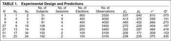
The experiment was designed with many features in mind, both from a logistical standpoint of experimental methodology and from a parametric standpoint of choosing the specific treatments and cost distribution. The experiment controlled all the parameters of the voter turnout game. After normalizing the payoffs (L and H), the game described in the previous section is fully characterized by N_A, N_B, and f. Since the three central hypotheses are the size effect, the underdog effect, and the competition effect, we were able to test all three by fixing f throughout the experiment, and varying only N_A and N_B. The payoffs were L = 5 and H = 105. We conducted elections with N ∈{3, 9, 27, 51}. For each of these electorate sizes, we have two subtreatments,³

When N = 3 these two treatments collapse into one treatment.

one where N_B = 2N_A and one where N_B = N_A+1. We refer to the former as the landslide treatment and the latter as the toss-up treatment. This modified 4 × 2 design is given in Table 1. We should indicate that we report payoffs in points, the units used in the experimental instructions and screens. In money, 100 points were equal to 37 cents. Average subject earnings were $33.60.

Our choice of the cost distribution, f, was dictated by two considerations, one theoretical and one logistical. Theoretically, there can be multiple quasi-symmetric equilibria for some cost distributions and some values of N_A and N_B. We desired a distribution with a unique quasi-symmetric equilibrium for all of our different (N_A, N_B) treatments, and one that was also easy to explain to naive subjects. A uniform distribution of voting costs ranging from 0 to 55 satisfies both of these desiderata. Since the payoff for making or breaking a tie is 50, voters who draw costs greater than 50 have a strict dominant strategy to abstain and voters with costs equal to 50 have a weakly dominant strategy to abstain. Equilibrium is unique for all our treatments, and the uniform distribution can be explained in terms of all costs within a give range being equally likely.⁴

It is not possible to show analytically that equilibrium is unique because of the two-sided nature of the problem. Since the space in which possible equilibria lie is only two dimensional, it is possible to do numerical grid searches to see if more than one equilibrium exists. For our parameters there is only one equilibrium. The details of the grid searches is reported at http://www.dklevine.com/papers/expvotebr.htm.

The unique Nash equilibrium turnout probabilities for the two groups are given in Table 1.

There were six main logistical challenges to conducting our experiment. First, we wanted a design that would be easy to explain to naive subjects who know nothing about the model and may be completely unfamiliar with abstract mathematical concepts such as probability distributions. Second, we wanted to control the information fiows so that individuals in the experiment would know their own costs but only the distribution of costs for the other individuals. Third, we wanted the parameters of the model and the voting rule to be as close to common knowledge as possible. Fourth, we wanted subjects to have an opportunity to gain experience, since past experiments have shown that behavior in games with pure strategy equilibria shows systematic convergence of behavior with experience. Fifth, we wanted a context-free design so that uncontrollable individual factors would not add another source of noise or introduce alternative explanations for the results. Sixth, we wanted a design that allowed within subject tests of the hypothesized effects, as well as between subject tests.

Our design generates a number of comparative statics hypotheses. For these hypotheses, we use the following notation. We denote the turnout rate for the underdog as a function of the sizes of group A and group B is by

and the turnout rate for the frontrunner by

COMPARATIVE STATICS HYPOTHESES

H1.: The Size Effect. Holding the relative size of the two groups constant, turnout in each party is decreasing in N. Formally, this implies 24 specific hypotheses in the form of pairwise inequalities. Two examples are

and

. Generally these inequalities take the form that if N<M; then

and

for j = A, B. In addition, there is the weaker hypothesis that total turnout is decreasing in N.

H2.: The Competition Effect. Holding the total size of the electorate constant, turnout in each party is decreasing in N_B − N_A. This gives us six specific hypotheses in the form of pairwise inequalities. They are

. Note that this hypothesis does not apply for the N = 3 treatment, since

in that case.

H3.: The Underdog Effect. For N > 3, turnout of party A is greater than turnout of party B. This gives us 6 specific hypotheses in the form of pairwise inequalities. They are

6),

H4.: Counter-example to the Underdog Effect. For N = 3, turnout of party A is less than turnout of party B. Specifically,

In addition to these comparative statics hypotheses, there are the specific quantitative hypotheses about turnout, given in Table 1. There are two additional sets of hypotheses about aggregate outcomes, listed in the last two columns of that table. The first is the equilibrium probability of a pivotal outcome. A pivotal outcome is one in which at least one voter is pivotal. That is, the outcome is either a tie or one vote away from a tie. It is noteworthy that if at least one voter is pivotal, then usually many voters are pivotal. In fact, in the case the vote is exactly a tie, all voters in both parties are pivotal, in the sense that if any single voter had voted differently, the tie would be broken.

It is straightforward to show that the comparative statics for the probability of a pivotal outcome are ordered exactly the same as the equilibrium turnout rates. This is true because in equilibrium the cutpoint for each party is proportional to the probability of making or breaking a tie. We denote this equilibrium probability π*(N_A, N_B). This generates a parallel set of hypotheses to H1−H2, which we call H5 and H6 and these parallel hypotheses are tested by looking at frequencies of pivotal events rather than turnout rates. The exact quantitative pivot probabilities are given in Table 1.

H5: The size effect on the frequency of Pivotal Events. Holding the relative size of the two groups constant, the frequency of pivotal events is decreasing in N. Formally, this implies 12 specific hypotheses in the form of pairwise inequalities. An example is π*(4, 5) > π*(13, 14). Generally these inequalities take the form that if N < M, then

and

H6: The competition effect on the frequency of Pivotal Events. Holding the total size of the electorate constant, the frequency of pivotal events is decreasing in N_A−N_B. This gives us 3 specific hypotheses in the form of pairwise inequalities: π*(4, 5) > π*(3, 6); π*(13, 14) > π*(9, 18), π*(25, 26) > π*(17, 34).

Finally, there is a separate set of hypotheses about the probability of an upset. We define an upset as an outcome of the election where the underdog receives more votes than the frontrunner. These upset probabilities are higher in toss-up races than in landslide races, but do not vary much with N. We denote the equilibrium upset probability by Q*(N_A, N_B), and the theoretical values for each treatment are in Table 1. This upset hypotheses are stated formally next:

H7: Upset Rates. The underdog is more likely to win outright in toss-up races than in landslide races, and these upset probabilities are increasing in N for the toss-up races. This generates nine specific hypotheses in the form of pairwise inequalities. Six of these are of the form

for N<M. The other three hypotheses are

, N=9, 27, 54.

In addition to hypotheses about aggregate behavior, the unique Bayesian Nash equilibrium also makes very sharp predictions about individual behavior. Specifically, all individuals should be using exact cutpoint rules. Moreover, these cutpoint rules should be precisely those corresponding to the turnout rates listed in Table 1. Obviously, hypotheses as sharp as this will inevitably be rejected. The cutpoint rules are pure strategies, so a single violation of the exact cutpoint rule by any subject in will completely reject the theory. Accordingly, we will pursue these hypotheses in the results section descriptively, rather than formally testing them. We also consider a bounded rationality model in which subjects follow a cutpoint rule stochastically—that is, they follow it most of the time, but violate it some of the time. This allows us to classify subjects according to their propensity to vote, which we expect to vary due to many diverse factors such as expectations about pivotal events, risk aversion, attitudes about group norms, social preferences, judgment fallacies and so forth.

There are also qualitative hypotheses that can be addressed at the individual level. In our design, subjects were in only one electorate size (3, 9, 27, or 51), but participated in a multiple elections, both toss-up and landslide, and participated as members of both the small group and the large group. This is explained in more detail in the next section. Accordingly, we address H2, H3, and H4 at the individual level as well as at the aggregate level.

EXPERIMENTAL PROTOCOL

Subjects were recruited by email announcement from a subject pool consisting of registered UCLA students. A total of 342 different subjects participated in the study. We conducted 19 separate sessions using networked computers at the CASSEL experimental facility.⁵

The software was programmed as server/client applications in Java, using the open source experimental software package called Multistage (http://multistage.ssel.caltech.edu/).

In each session, N was held fixed throughout the entire session. For the N>3 sessions, there were two subsessions of 50 rounds each; one subsession was the toss-up treatment and the other subsession was the landslide treatment. The sequencing of the two treatments was done both ways for each N. Before each round, each subject was assigned to either group A or group B and assigned a voting cost, drawn independently from the uniform distribution between 0 and 55, in integer increments. Therefore, each subject gained experience as a member of the majority and minority party for exactly one value of N, and participated in both 50 landslide and 50 toss-up elections. Instructions were read aloud so everyone could hear, and Powerpoint slides were projected in front of the room to help explain the rules and to make all the common knowledge to the extent possible. After the instructions were read, subjects were walked through two practice rounds with randomly forced choices and then were required to correctly answer all the questions on a computerized comprehension quiz before the experiment began. After the first 50 rounds, a very short set of new instructions were read aloud, explaining that the sizes of group A and group B would be different for the next 50 rounds.

The wording in the instructions was written so as to induce as neutral an environment as possible.⁶

A sample of the instructions from one of the 27-person sessions is in the Appendix. All of the instructions together with the data from all sessions can be found on the Web at http://www.dklevine.com/workshop/cost-vote/index.php

There was no mention of voting or winning or losing or costs. The labels were abstract. The smaller group was referred to as the alpha group (A) and the larger group was referred to as the beta group (B). Individuals were asked in each round to choose X or Y. If more members of A(B) chose X than members of B(A) chose X, then each member of A(B) received 105 and each member of group B(A) received 5. In case of a tie, each member of each group received 55 (the expected value of a fair coin toss). Therefore, voting corresponded to “choosing X” and abstaining corresponded to “choosing Y.” The voting cost was referred to as a “Y bonus” and was added to a player's earnings if that player chose Y instead of X in an election. Therefore, the voting cost was implemented as an opportunity cost. If a player chose X, that player did not receive their Y bonus for that election. Bonuses were randomly redrawn in every round, independently for each subject, and subjects were only told their own Y bonus.⁷

We ran two additional sessions with n=9, where the instructions were presented in the context of a voting decision in elections. The results were nearly identical and are discussed in the results section.

The N = 3 sessions were conducted slightly differently. First, there were only 50 rounds, since the toss-up and landslide treatments were identical. Second, the sessions were conducted with either 12 or 15 subjects, who were randomly rematched each round into subgroups of 3 each period, before being assigned a party and a voting cost. This allowed us to obtain a comparable number of subjects for the N = 3 treatment as the other treatments.

RESULTS

Aggregate Results

The analysis of results at the aggregate level is carried out at two levels. First, we look at the empirical turnout rates, and how they vary with respect electorate size, the competitiveness of the election, and whether voters are from the majority or minority parties. This enables us to address hypotheses H1−H4. Next, we focus on outcomes and show how the empirical frequencies of pivotal events, upsets, and election margins vary with electorate size and electoral competitiveness.

Turnout Rates.

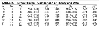
Table 2 displays and Figure 1 graphs for each party and each treatment the observed turnout rates (denoted

with standard errors in parentheses) alongside the Nash equilibrium values.⁸

Columns 6 and 9 relate to the QRE analysis and are discussed later. The standard errors assume independence of the observations, which is consistent with the theoretical model we are testing. However, there may be dependence due to multiple observations of the same individual. Therefore, these should represent a lower bound on the standard errors. We take a second look at this by examining individual effects in the next section.

Out of 37 pairwise comparisons of turnout rates, 35 have the same sign as predicted by the theory. Hypotheses about the competition effect (H2), the underdog effect (H3), and the three-voter counter-example to the underdog effect (H4), are supported without exception. That is, all pairwise comparisons of turnout rates for those hypotheses are the same as predicted by the theory. Particularly noteworthy (and surprising to us) is the support for H4: the minority turns out less than the majority in only one instance, which is precisely the one predicted by the theory (N_A=1, N_B = 2). In all other cases, there is greater turnout by the minority party.

Minority and Majority Party Turnout Rates as Function of Electorate Size

The size effect, H1, is supported with the exception of the comparison of turnout in tossup races with 27 versus 51 voters. In that comparison, both the minority and majority parties vote slightly more often in the 51 case than the 27 case, but these are both quantitatively smaller than all other differences (.005 and .006, respectively), and neither is large relative to sampling variation as measured by the standard errors.

Quantitatively, the turnout rates we observe for the smallest electorate (N = 3), are lower than predicted by theory, turnout rates for somewhat larger electorates (N = 9) are approximately equal to the Nash equilibrium value, whereas turnout rates for the largest electorates (N = 27, 51) are higher than predicted by theory. As a general rule, we find that turnout rates are closer to 0.5 than theory predicts. This mirrors findings by Goeree and Holt (2005) for a broad class of games with a similar structure to our voter turnout experiments.⁹

They study binary choice games such as threshold public goods games, where observed contribution rates tend to exceed the equilibrium predictions when the equilibrium is below .5, and are too low when the equilibrium is above .5%.

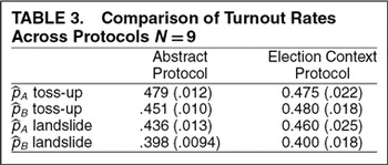
We conducted two additional sessions with N = 9, as a robustness check for the abstract context. In these session, we changed the terminology of “X” and “Y” to “Vote” and “Abstain.” Each round was referred to as an election, groups were called parties, and so forth. The turnout rates are given in Table 3, side by side with the results from sessions run with an abstract protocol, with standard errors in parentheses. Three differences are positive and one is negative. All are small in magnitude, and are small compared to the sampling variation in the Election Context Protocol estimates as measured by the standard errors.

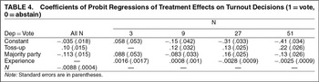
We also report the results of a simple probit regression of the probability a voter turns out as a function of which party the voter was in (majority or minority), whether the or not the race was a toss-up, and the size of the electorate. The results are given in Table 4, along with t-statistics. The coefficients on all three variables are highly significant and have the predicted signs: negative effect of majority party membership, positive effect of toss-up, and negative effect of electorate size. In this estimation and in subsequent individual level analysis, we include observations from the two election context sessions.

Because the observed turnout frequencies in the sessions with N = 27 and N = 51 were significantly different than the Nash equilibrium turnout rates, we also included a variable for experience, which takes on values from 1 to 50, corresponding to the round number. Recall that each treatment in each session lasted for 50 rounds. We hypothesize that behavior should converge in the direction of Nash equilibrium, a phenomenon that has been widely observed in game theory experiments. However, the effect of experience should be different depending on N. For N = 3 and N = 9, aggregate turnout rates are almost exactly equal to Nash prediction, so we do not expect experience to change behavior. The experience coefficient should be positive for N = 27 and N = 51, since observed turnout was above equilibrium level. Because the expected effects differ across N, we estimate the effect separately for each N.

The results are also given in Table 4 and provide some support for the idea that behavior is adjusting in the direction of equilibrium. For both the N = 27 and the N = 51 sessions, the coefficient on experience is precisely estimated and negative. In both cases, there was approximately a 5-percentage-point drop in turnout between the first and last rounds, controlling for party and tossup. For N = 3 and N = 9, the coefficient is virtually equal to zero, as expected.

Upsets, Pivotal Events, and the Distribution of Margins of Victory.

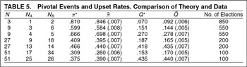
Table 5 displays the observed and equilibrium frequencies of pivotal events, π, for each treatment and the observed and equilibrium upset rates, Q. Standard errors are reported in parentheses.

Overall, the data provide strong support for hypotheses H5, H6, and H7. Every single one of the 15 size-effect inequalities for pivotal events (H5) are observed in the data, and all 3 of the competition-effect inequalities for pivotal events (H6) are also found. The same is true for the 9 predicted inequalities for upsets (H7), with only one exception:

, but the difference is only 0.005.

Also noteworthy is the fact that the data tracks the theory very closely quantitatively, as well as qualitatively. Indeed the quantitative departures from theory are behaviorally meaningless. To illustrate this, Figure 2 graphs the observed and predicted values of π and Q for all treatments. A simple linear regression of observed on theoretical rates, using all 14 data points in the figure (including both pivot probabilities and upsets) produces an intercept equal to −0.01, a slope equal to 1.03, and an R² equal to .99.

Pivotal Events and Upsets

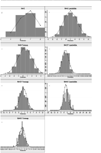
The upset frequencies and empirical pivot probabilities represent two different quantile statistics of the distribution of margins of victory. We also examined the behavior of election margins more generally. Figure 3 compares the observed distributions of victory margins in the data with the theoretical distributions at the Nash equilibrium, for each treatment. Clearly, the data are a very close match to the theory. Since the participation rate in the data and that predicted by the theory are very close, it is perhaps not that surprising that the distribution of vote margins is quite similar between the data and the theory. However, it is noteworthy that the distribution closely matches the theoretical prediction even in the 51-voter treatments, where we observed significant overvoting.

Distribution of Party B's Margin of Victory: Theory (line) versus Data (bar)

Individual Results

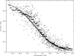
We turn now from examining the aggregate implications of the theory to implications for individual behavior. Nash equilibrium predicts that all subjects should follow a common cutpoint rule—that is, the smooth logit curve in Figure 4 should be a vertical line at zero. In fact, as that graph shows, individual behavior shows substantially more variation than Nash equilibrium allows. We now look in more detail at the play of specific subjects.

Turnout Rates as Function of Cost, Compared to Logit Response with λ=7

Estimating Individual Cutpoints.

To summarize the behavior of individual subjects, we assume that each subject is following a cutpoint rule and attempt to estimate subject by subject what that rule is. Recall that best responses always take the form of cutoff rules, whereby a voter should vote if and only if the cost they draw is greater than or equal to a critical cost level, c.

For each treatment and each subject, we estimated cutpoint rules in the following simple way. For each subject i and treatment j, we have K_ij observations of cost, decision pairs (c_t, d_t). Fix a cutpoint 0 ≤ c_ij ≤ 55. If for observation t in this sample of K_ij observations we have

we say that observation t is consistent with the cutpoint c_ij. Otherwise, we say that observation t is an error with respect to the cutpoint c_ij.¹⁰

Alternatively, one could discount the error by how close the cost is to the cutpoint. This could be done for example by estimating for each ij pair a logit choice function and defining the estimated cutpoint as the point at which the estimated logit choice probability is exactly .5.

The estimated cutpoint,

is the cutpoint that one that minimizes the number of errors.¹¹

In case there are multiple error-minimizing cutpoints, we use the average of them.

Using this procedure, we can produce a distribution of cutpoints for each treatment and a distribution of error rates for each treatment. The density for error rates is shown in Figure 5. As can be seen, there are errors, but in general not so many, indicating that to a reasonable approximation individuals followed consistent cutpoint rules. More than one-third of the subjects are almost perfectly classified (>95% of decisions correctly classified) more than one-half are nearly as well classified (>90%), and for nearly all subjects the percent of decisions correctly classified is greater than 80%.

Distribution of Misclassification Rates

Figure 6 graphs the cumulative distribution function for the estimated individual cutpoints of majority voters in all the landslide elections. There is one curve graphed for each N treatment. This illustrates several properties. First, it reflects the comparative statics of the size variable, with the distribution of cutpoints for smaller elections stochastically dominating the distribution of cutpoints for larger elections, in most cases. Second this stochastic dominance is not observed between N = 27 and N = 51, consistent with the aggregate data which showed little difference between turnout in those elections. Third, there is a lot of heterogeneity. Recall that in the Nash equilibrium, all voters should be using the same cutpoint, in which case the cumulative distribution functions of individual cutpoints should be step functions at the Nash equilibrium cutpoint. Clearly that is not the case. This heterogeneity will be partially accounted for later in the paper, in the section on quantal response equilibrium.¹²

The cumulative distribution function graphs for minority voters and the tossup elections also share these properties. These graphs are reproduced in the working paper version, available on the web.

Landslide Majority Individual Cutpoint CDF

Toss-ups and Landslides.

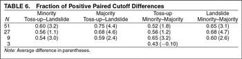
We turn now to comparative statics at the individual level. For the experiments with N>3, we have four paired observations for individuals: holding fixed whether the individual is in the minority or majority, we can consider the difference in their cutpoint between a toss-up and a landslide, holding fixed whether the election is a toss-up or a landslide, we can consider the difference in their cutpoint between being in the minority and the majority. According to the theory, all of these differences should be positive (except for N = 3). Table 6 reports the fraction of these differences that are positive. As can be seen, this is always above 50% and generally 60% or higher. This is reinforced by the average size of these differences, shown in parentheses, all with the correct sign.

QUANTAL RESPONSE EQUILIBRIUM MODEL OF TURNOUT

In this voter participation game, subjects with cutpoints close to the equilibrium cutpoint are nearly indifferent between voting and abstaining. Consequently, very small errors in their judgment about the pivot probabilities, or other factors, could lead them to make a suboptimal decision. With this in mind, it makes sense to explore models such errors are possible and where the probability of such errors are derived endogenously in the model.

Logit Equilibrium

One alternative is to allow a small amount of bounded rationality and assume that players are not optimizing but instead choose according to a Logit stochastic choice rule. If they also have rational expectations, then it is called the Logit quantal response equilibrium model. In a quantal response equilibrium, decision making no longer follows a deterministic cutpoint rule. Rather, a voter's turnout probability is a continuous strictly increasing function of voting cost, τ(·), which is equal to .5 precisely at the voting cost at which the voter is exactly indifferent between voting and abstaining. If π_j is the probability a voter in party j is pivotal (which will generally be different for minority and majority voters), then in a logit equilibrium such a voter's turnout probability, if his voting cost is c follows the formula:

where λ is the logit response parameter. Integrating over all possible voting costs, we obtain the voter's ex ante turnout probability:

There will be one such equation for each party, analogous to equations 1 and 2 in the Nash equilibrium analysis.¹³

The Nash equilibrium analysis is equivalent to the limiting case of λ=∞.

Since this is an equilibrium model, π_j is determined endogenously, and will depend on λ, since it depends on

, which depends on τ_j, which in turn depends on λ. The equilibrium pivot probabilities, {π_A(λ), π_B(λ)}, are then computed using formulas similar to equations 3 and 4.

The logit response parameter, λ is a free parameter corresponding to the slope of the logit response curve. We estimate λ to fit the data. To avoid overfitting, we constrain λ to be the same in all treatments. Using the data, it is easy to compute the maximum likelihood estimate of λ based on the pooled data from all treatments. We do this by actually computing the logit equilibrium of each game for a grid of values of λ, and then can directly construct the likelihood function of our pooled data, as a function of λ. This yields a maximum likelihood estimate equal to

.¹⁴

Costs and benefits were scaled using experimental points divided by 100.

We then use that estimated value,

, along with the actual draws of voting costs, to compute for each treatment and each part, theoretical QRE turnout rates, denoted p^λ=7. These are given in two columns of Table 2 and also displayed in Figure 1. Two observations are clear. First, the QRE model fits the data better. Second, the QRE model provides exactly the right qualitative correction to the Nash model. Recall that the Nash model underpredicted turnout in larger elections and overpredicted turnout in small elections, and did fairly well for intermediate-sized elections. The QRE predicts less turnout than Nash equilibrium in the smallest election, and more turnout than Nash equilibrium in the large elections. QRE also predicts even greater amounts of overvoting (relative to Nash), as the size of the election becomes larger and larger, which is what we observed in the data.

The quantal response equilibrium we consider also provides a partial explanation for the observed heterogeneity of estimated individual cutpoints, as well as the classification errors. Because subjects are choosing stochastically, we will inevitably observe classification errors for some subjects. Furthermore, the combination of stochastic choice and the relatively small (random) sample of assigned voting costs for each voter will result in the measurement of significant heterogeneity of individual estimated cutpoints, using the method described in the earlier section.

Normalized Voting Cost Analysis

As an alternative way to see how well the logit choice model is capturing voter behavior, Figure 4 graphs turnout rates by “normalized” voting cost. For each treatment and each party, we define a normalized voting cost as the difference between a voter's actual voting cost and the logit equilibrium cutpoint (for λ=7). Thus, for example, if the QRE cutpoint for an A voter in some treatment were, say, 15, and their actual cost were 25, their normalized voting cost would be 10. Thus our normalization allows us to display all the voting behavior in a single graph. According to the logit QRE, the voting probabilities should follow a logit curve, which is the smooth decreasing curve in the figure (for λ=7). The decreasing step-function curve averages the data across normalized cost intervals of .03.

Asymptotic Voter Turnout in QRE

We cannot carry out experiments with millions of voters, but we can ask what the theory and our estimates predict in very large elections.

Examining first Nash equilibrium, it is well known that as the population increases, participation falls to zero. Suppose that for one of the parties it does not. Then for that party, the probability of being pivotal must fall to zero. This in turn implies that the optimum threshold for participation is falling to zero, leading to a participation rate that falls to zero, contradicting the original hypothesis. Indeed, this is a version of the “paradox of voter participation.”

By way of contrast, the quantal response model is much better behaved. For a given value of λ we can compute the participation rate:

where the QRE pivot probability, π_j, is endogenous. However, just as in the Nash equilibrium, in a large population, the QRE probability of being pivotal is approximately zero, so we have the following large population approximation for

We may then compute the asymptotic participation rate as a function of λ. In particular, for the value of λ estimated with our data, the asymptotic participation rate is 17%. For the participation rate to fall to 5%, for example, would require λ = 28, which is an order of magnitude higher than we estimate.

To compare with elections in the field, it is more reasonable to use a lower distribution of voting costs that our experiment. The average voting cost in our experiment is equal to one-quarter the value of being a “dictator” over the outcome of the election, which is probably several orders of magnitude too small for many important elections where voters have intense preferences over the alternatives or candidates. To consider lower distributions of voting costs, suppose that the maximum voting cost is C and the distribution is uniform. Then the asymptotic expected turnout in the Logit QRE is equal to

For λ = 7 this expression implies 48% turnout (42% if λ=28) when C = .02.

More generally, if the distribution has an arbitrary shape, and the fraction of voters with costs less than or equal to C is f, then we can compute voter turnout by multiplying by f. So, for example, if only 80% of voters have costs below .02 and λ=7, the corresponding asymptotic turnout is .8 × .48 = .384. In fact, for all values of λ, turnout percentage converges to 50% as C converges to 0 in the uniform case, and as the random variable representing the cost distribution converges to zero in probability in the general case. In other words, even with incredibly rational voters (λ > 100, for example), very high asymptotic turnout rates can be supported provided the distribution of costs is low (or the stakes are very high). It is only in the knife-edge case of perfectly rational voters (λ = ∞) that the turnout paradox arises.

CONCLUSIONS

There are seven main findings from this voter-turnout experiment.

First, and most important, all of the comparative statics from the standard Bayesian Nash equilibrium model of instrumental strategic voting were strongly supported by the data. We find strong evidence for the size effect, the competition effect, and the underdog effect. The evidence is based on turnout rates, frequency of pivotal events, and upset probabilities. It is further supported by individual-level analysis that was possible because we can compare an individual subject's decisions in multiple treatments.

Second, voters are highly responsive to voting cost, with turnout rates declining sharply with the cost of voting. As a first approximation, most voters use cutpoint strategies, as predicted by the theory.

Third, a close look at individual behavior reveals that few voters use exact deterministic cutpoint strategies, choice behavior appears to have a stochastic element. This replicates a finding from several other studies of games with binary choices and continuous types, where best-response rules are cutpoint strategies.¹⁵

See, for example, Casella, Gelman, and Palfrey 2006, Palfrey and Prisbrey 1997, and Palfrey and Rosenthal 1991.

Fourth, voters were less responsive to changes in the parameters of the environment than the equilibrium. In particular, this resulted in turnout rates that were too low for N = 3 and that exceeded the Nash equilibrium rates for the larger groups, with overvoting especially noticeable in the N = 51 treatment.

Fifth, an equilibrium approach based on the logit version of QRE, which incorporates the kind of stochastic choice observed at the individual level, provides a significant improvement in fit over the Nash model, as well as providing an explanation for undervoting (relative to Nash) in small elections and overvoting in large elections. Furthermore, the responsiveness of participation rates to voting costs is tracked very closely by a logit curve (Figure 4). Nonetheless, the logit QRE model may not fully account for the magnitude of overvoting in the largest elections of our sample, unless there are higher error rates (smaller λ) in larger elections, a possibility which does not have an obvious rationale a priori.

Sixth, we projected our QRE estimates to larger elections, and show that QRE can account for substantial turnout for larger elections. We ourselves were quite surprised to discover that, with our estimate of the logit QRE and the experiment's distribution of voting costs, 17% turnout would be projected in arbitrarily large elections. For more realistic voting costs turnout is on the order of 50%. Thus QRE effectively resolves the “paradox” without the addition of utility terms such as citizen duty or other ad hoc rationalizations. That is, substantial turnout in large elections is consistent with equilibrium behavior of highly (but not perfectly) rational voters.

Seventh, the experiment was conducted in a neutral abstract context with no mention of voting, or winning, or parties or elections. In the two extra sessions conducted specifically in a voting context, subject behavior was the same as the abstract context. Hence the phenomena we observe apparently are not limited to elections, but are more general. In particular the observation of overvoting relative to the equilibrium cannot be easily dismissed by appealing to arguments such as citizen duty, high school civics classes, or fear that one's spouse of workmates will castigate one for not voting.

The challenge now is to come up with an explanation of over voting that is not specific to elections, but applies more broadly to participation games in general. The one alternative explored here, QRE, provides a partial explanation, but undershoots the overvoting in large elections. Another explanation we have considered, that voters systematically overestimate the probability of being pivotal, is directly contradicted by the N = 3 data, where we observe undervoting. For the same reason, our data also fail to support group-specific altruism models, and also the group-utilitarian approach of Harsanyi (1980), recently proposed as an explanation of high voter turnout by Feddersen and Sandroni (2002), and studied empirically by Coate and Conlin (2004). Another alternative model minimax regret is due to Ferejohn and Fiorina (1974). That model is easily rejected, because it implies that turnout should independent the probability of being decisive, which contradicts the size effect, the competition effect, and the underdog effect.

We conjecture that some kind of mixture of models such as these, which would include a variety of behavioral types, will ultimately be needed for a more complete explanation of this phenomenon and the heterogeneity we observe. One framework for building and estimating such models has been developed by El-Gamal and Grether (1995). However, developing a specification of types for the voting context that is not ad hoc would be a challenge, and computation and estimation of such a model may be difficult.

In conclusion, the strength of the comparative statics results should not be understated. The fact that the experiment clearly supports the three main equilibrium comparative static effects (size, competition, and underdog) in participation games, and the finding that voters use approximate cutpoint strategies demonstrates that voting behavior is highly strategic, with voters responding to both the cost of voting and the probability of being pivotal.

APPENDIX: SAMPLE INSTRUCTIONS FOR 9 PERSON SESSION

Thank you for agreeing to participate in this research experiment on group decision making. During the experiment we require your complete, undistracted attention. So we ask that you follow instructions carefully. Please do not open other applications on your computer, chat with other students, read books, or do homework.

For your participation, you will be paid in cash, at the end of the experiment. Different participants may earn different amounts. What you earn depends partly on your decisions, partly on the decisions of others, and partly on chance. So it is important that you listen carefully and fully understand the instructions before we begin. There will be a short comprehension quiz after the upcoming practice round, which you all need to pass before we can begin the paid sessions.

The entire experiment will take place through computer terminals, and all interaction among you will take place through the computers. It is important that you not talk or in any way try to communicate with other participants during the experiments, except according to the rules described in the instructions.

We will start with a brief instruction period. During the instruction period, you will be given a complete description of the experiment and will be shown how to use the computers. If you have any questions during the instruction period, raise your hand and your question will be answered out loud so everyone can hear. If any difficulties arise after the experiment has begun, raise your hand, and an experimenter will come and assist you privately. Please open your envelope and remove the Record Sheet. Do not lose this Record Sheet, as you will need the sheet throughout the experiment to record your earnings.

This experiment will begin with two brief practice sessions to help familiarize you with the rules. The practice session will be followed by two different paid sessions. Each paid session will consist of 50 rounds. At the end of the last paid session, you will be paid the sum of what you have earned in the two paid sessions, plus the show-up fee of $5.00. Everyone will be paid in private, and you are under no obligation to tell others how much you earned. Your earnings during the experiment are denominated in POINTS. Your DOLLAR earnings are determined by multiplying your earnings in POINTS by a conversion rate. In this experiment, the conversion rate is 0.0037, meaning that 100 POINTS is worth 37 cents.

There are nine participants in today's experiment. You will participate in two brief practice sessions and then two paid sessions of 50 rounds each.

Please turn your attention to the screen at the front of the room. We will demonstrate how the rounds are played. (SHOW SCREEN 1 [menu].) Everyone should have a screen like the screen projected on stage. If you have something different from what is projected on stage, please raise your hand and the staff will assist you. [CHECK TO SEE IF ANYONE RAISES THEIR HAND.]

Please do not begin unless we tell you to do so. Please have your attention focused on the stage during this demonstration period. Please click on the MENU icon. This will bring up screen 2 showing the icons underneath. (SHOW SCREEN 2 [icons].) On this second screen, click on the MULTISTAGE CLIENT icon. A pop-up window will appear right in front of you. (SHOW SCREEN 3 [client information].) Enter your first and last name in the box that appears and then click submit. You will then see screen 4. (SHOW SCREEN 4 [initializing].)

Once everyone has logged in, you will be randomly assigned to one of two groups the ALPHA group or the BETA group. You will see screen 5 (SHOW SCREEN 5 [user interface].) At the top of the screen is your id number. Please record this on your Record Sheet. Below this the screen informs you which group you are in and how many members there are in each group. In this practice session, the ALPHA group has 4 members and the BETA group has 5 members. Next on the screen is a table, describing how your earnings depend on your choice of either X or Y and on which group has the most members choosing X. The display in front of the room shows you what the screen looks like for a member of the Alpha group. It also tells you what your Y bonus is. We will explain what this means in a moment.

You will choose either X and Y by highlighting the corresponding row label and clicking with your mouse. (SHOW SCREEN 6x and 6y and 7 [showing highlighting].) Your earnings are computed in the following way. It is very important that you understand this, so please listen carefully. Suppose you choose X. If your group has more members choosing X than the other group, then you will earn 105 points, if both groups have the same number of members choosing X, then you will earn 55 points, and if the other group has more members choosing X than your group, then you will earn 5 points.

Alternatively, suppose you choose Y. If your group has more members choosing X than the other group, then you will earn 105 points plus your Y bonus, if both groups have the same number of members choosing X, then you will earn 55 points plus your Y bonus, and if the other group has more members choosing X than your group, then you will earn 5 points plus your Y bonus. The amount of your Y-bonus is assigned randomly by the computer and is shown in the fourth line down from the top of your screen. In any given round you have an equal chance of being assigned any Y-bonus between 0 and 55 points. Your Y-bonus in each round does not depend on your Y-bonus or decisions in previous rounds, or on the Y-bonuses and decisions of other participants. Since Y-bonuses are assigned separately for each participant, different participants will typically have different Y-bonuses. While you are told your own Y-bonus, you are never told the Y-bonuses of other participants. You only know that each of the other participants has a Y-bonus that is some number between 0 and 55.

Here is an example: suppose that one member of the ALPHA group chose X and two members of the BETA group choose X. Then the BETA group has more members choosing X than the ALPHA group. Each member of the ALPHA group who chose X earns 5 points; each member of the ALPHA group who chose Y earns 5 points plus his or her own personal Y-bonus; the members of the BETA group who chose X earn 105 points, and each member of the BETA group who chose Yearns 105 points plus his or her personal Y-bonus.

The bottom of the screen contains a history panel. During the various sessions and rounds, this panel will be updated to refiect the history of your past sessions.

After you and the other participants have all made your choices of X or Y the screen will change to highlight the row corresponding to your own choice, and the column of the group which had the greatest number of members choose X.

At the end of each round until the session ends, you will be randomly divided between groups and will have the opportunity to choose between X and Y. In other words, you will not necessarily be in the same group during each round. At the end of each session, you will see a screen summarizing the amount that you earned. (SHOW SCREEN 8 [match complete].) If you have any questions at this time, please raise your hand and ask your question so that everyone in the room may hear it.

PRACTICE SESSION [BRING UP PAYMENT SCREEN FOR PRACTICE SESSION] We will now give you a chance to get used to the computers with a short practice session. Please take your time, and do not press any keys or use your mouse until instructed to do so. You will NOT be paid for this session; it is just to allow you to get familiar with the experiment and your computers.

If your ID number is even, please highlight the Y row and click; if your ID number is odd, please highlight the X row and click. Once everyone has made their selection, the results from this first practice round are displayed on your screen. Remember, you are not paid for this practice round.

We will now proceed to the second practice round. Notice that you may have been reassigned to a new group, since the group assignments are shuffled randomly between each round. Please make the opposite choice from the choice you made in the first practice round. That is, if your ID number is even, please highlight the X row label and click; if your ID number is odd, please highlight the Y row label and click. Once everyone has made their selection, the results from this second practice round are displayed on your screen.

Since this is the end of the practice round, your total earnings for this practice session are displayed on your screen in points (though of course, you wont actually receive that money). We have now completed the practice session.

[QUIZ] You will notice that a quiz has popped up on your screen. Please read each question carefully and check the correct answer. Once everyone has answered the questions correctly, you may all go on to the second stage of the quiz. After successfully completing the second round of questions, we will commence with the first paid session. If you have difficulty with the quiz or have other questions please your hand. [END QUIZ]

The first paid session will follow the same rules as the practice session. Let me summarize those rules before we start. Please listen carefully. In each round of this session, four players will be randomly assigned to the Alpha Group, and five players will be assigned to the Beta Group. You may choose X or Y. As you can see on the table of this screen, if you choose X, your payoff will be 105 POINTS if your group has more members choosing X than the other group, 5 POINTS if your group has fewer members choosing X, and 55 POINTS if it is a tie. If you choose Y, you will also receive the Y-bonus shown on your screen.

There will be 50 rounds in this session. After each round, group assignments will be randomly reshuffled. Therefore, in some rounds you will be in the Alpha group, and in other rounds you will be in the Beta group. In either case, everyone is told which group they are in before making a choice of X or Y. Are there any questions before we begin the first paid session [Answer questions.] Please pull out your dividers.

SESSION 1 We will now begin with session 1. Do not click anything else on the screen until you are told to do so. [BRING UP PAYMENT SCREEN FOR SESSION 1] Please begin. (Play rounds 1–50.) Session 1 is now over. Please record your total payoffs for this session on your record sheet. [WAIT FOR STAFF TO VERIFY PARTICIPANTS RECORD SHEET]

SESSION 2 We will now begin session 2. [BRING UP PAYMENT SCREEN FOR SESSION 2] The second paid session will be slightly different from the first session. Let me summarize those rules before we start. Please listen carefully. In each round of this session, three players will be randomly assigned to the Alpha Group and six players will be assigned to the Beta Group. You may choose X or Y. As you can see on the table of this screen, if you choose X, your payoff will be 105 POINTS if your group has more members choosing X than the other group, 5 POINTS if your group has fewer members choosing X, and 55 POINTS if it is a tie. If you choose Y you will also receive the Y-bonus shown on your screen.

There will be 50 rounds in this session. After each round, group assignments will be randomly reshuffled. Therefore, some rounds you will be in the Alpha group and other rounds you will be in the Beta group. In either case, everyone is told which group they are in before making a choice of X or Y. Are there any questions before we begin the second paid session?

Please Begin. (Play rounds 1–50.) Session 2 is now over. Please record your total payoffs for this session on your record sheet.

We thank National Science Foundation Grants SES-0314713 and SES-0079301 for financial support. We are grateful to Brian Rogers, Richard Scheelings, StephanieWang, and Rumen Zarev for research assistance. We thank three referees, Navin Kartik, and seminar participants at Caltech, Duke University, NYU, Princeton, UC Berkeley, and University of Rochester for comments.

References

Casella Alessandra, Andrew Gelman, and Thomas Palfrey. 2006. “An Experimental Study of Storable Votes.” Games and Economic Behavior 57 (October): 123– 54.Google Scholar

Cason Timothy, and Vai-Lam Mui. 2005. “Uncertainty and resistance to reform in laboratory participation games.” European Journal of Political Economy 21 (September): 707– 37.Google Scholar

Coate Stephen, and Michael Conlin. 2004. “A Group Rule-Utilitarian Approach to Voter Turnout: Theory and Evidence.” American Economic Review 94 (December): 1476– 1504.Google Scholar

Downs Anthony. 1957. An Economic Theory of Democracy. New York: Harper and Row.

El-Gamal Mahmoud, and David Grether. 1995. “Are People Bayesian? Uncovering Behavioral Strategies.” Journal of the American Statistical Association: Applications and Case Studies 90 (December): 1137– 45.Google Scholar

Feddersen Timothy, and Alvaro Sandroni. 2002. “A Theory of Participation in Elections with Ethical Voters.” Working Paper. Northwestern University.

Ferejohn John, and Morris Fiorina. 1974. “The Paradox of Not Voting: A Decision Theoretic Analysis.” American Political Science Review 68 (June): 525– 36.Google Scholar

Goeree Jacob, and Charles Holt. 2005. “An Explanation of Anomalous Behavior in Models of Political Participation.” American Political Science Review 99 (May): 201– 13.Google Scholar

Green Donald, and Ian Shapiro. 1994. Pathologies of Rational Choice Theory. New Haven: Yale University Press.

Grofman Bernard. 1993. “Is Turnout the Paradox that Ate Rational Choice Theory?” In Information, Participation, and Choice. ed. B. Grofman. University of Michigan Press: Ann Arbor.

Grosser Jens, Tamar Kugler, and Arthur Schram. 2005. “Preference Uncertainty, Voter Participation and Electoral Efficiency: An Experimental Study.” Working Paper. University of Cologne.

Grosser Jens, and Arthur Schram. 2006. “Neighborhood Information Exchange and Voter Participation: An Experimental Study.” American Political Science Review 100 (2): 235– 48.Google Scholar

Hansen Steven, Thomas Palfrey, and Howard Rosenthal. 1987. “The Downsian Model of Electoral Participation: Formal Theory and Empirical Analysis of the Constituency Size Effect.” Public Choice 52 (1): 15– 33.Google Scholar

Harsanyi John. 1980. “Rule Utilitarianism, Rights, Obligations, and the Theory of Rational Behavior.” Theory and Decision 12 (June): 115– 33.Google Scholar

Palfrey Thomas, and Jeffrey Prisbrey. 1997. “Anomalous Behavior in Linear Public Goods Experiments: How Much and Why?” American Economic Review 87 (December): 829– 46.Google Scholar

Palfrey Thomas, and Howard Rosenthal. 1983. “A Strategic Calculus of Voting.” Public Choice 41 (1): 7– 53.Google Scholar

Palfrey Thomas, and Howard Rosenthal. 1985. “Voter Participation and Strategic Uncertainty.” American Political Science Review 79 (March): 62– 78.Google Scholar

Palfrey Thomas, and Howard Rosenthal. 1991. “Testing Game-Theoretic Models of Free Riding: New Evidence on Probability Bias and Learning.” In Laboratory Research in Political Economy, ed. T. Palfrey. University of Michigan Press: Ann Arbor.

Schram Arthur, and Joep Sonnemans. 1991. “Why people vote: Free riding and the production and consumption of social pressure.” Journal of Economic Psychology 12 (December): 575– 620.Google Scholar

Schram Arthur, and Joep Sonnemans. 1996. “Why people vote: Experimental. Evidence.” Journal of Economic Psychology 17 (August): 417– 42.Google Scholar

Schram Arthur, and Joep Sonnemans. 1996. “Voter Turnout as a Participation Game: An Experimental Investigation.” International Journal of Game Theory 25 (September): 385– 406.Google Scholar