1 Introduction
Over the last years, the number of available linked knowledge data sets as well as the size of each single data set has undergone an exponential growthFootnote 1 . In the beginnings, stores designed for linked data query and retrieval could easily deal with the amount of data available by either using in-memory stores or by mapping the graph data onto existing relational database technologies. With the amount of linked open data surpassing the computing power of a single central device unit, it became inevitable to distribute the workload onto several device units. Furthermore, dedicated main memory systems were developed to ensure low access times. However, future graph stores will have to cope with significantly larger data sets due to exponential growth. Eventually, this development will surpass the performance of today’s main memory graph stores. The main reason for this lies in the access delay of main memory, which did not evolve at the same rate as computation power. Consequently, the so-called memory wall issue (Wulf & McKee, Reference Wulf and McKee1995) emerged. On contemporary systems, this means that a single Central Processing Unit (CPU) executes about 100 instructions until it receives previously requested data from the main memory. For computationally intensive problems, which require many instructions per single data element, this performance penalty can be neglected. However, in graph stores computationally cheap filter operations are dominant. This makes such systems much more vulnerable to the memory wall issue. Furthermore, the problem becomes even worse if distribution is introduced, as in multi-core environments all CPUs need to share a single main memory interface. Hence, we identify the memory wall effect as the main problem of future graph stores. This issue needs to be addressed to enable both higher performance and scalability.
Spatial computers present a promising alternative to address this issue as they introduce a new way of how data are stored and processed. In more detail, in spatial computers physical space is not an issue that is neglected, but is exploited to enable more efficient storage and distributed processing (DeHon et al., Reference DeHon, Giavitto and Gruau2007). The Paintable Computers of Butera (Reference Butera2002) and the GraphStep system of Delorimier et al. (2011) are two good examples for spatial computers. The former consists of small device units mixed into paint and then put on an arbitrary object. As device units can only communicate to nearby units, the surface of the object becomes a spatial computer. The latter is a distributed graph processing framework for Field Programmable Arrays (FPGAs). The authors pointed out that FPGAs are spatial computers and spatial geometry must be considered. To this end, the GraphStep system realizes a spatially aware approach. This work follows a similar, but broader approach and focuses on graph stores operating in one-dimensional (1D), 2D and 3D physical space. In particular, we introduce the term Spatially Aware Graph Stores for hybrid graph stores that operate in a spatial computer environment.
In the course of an efficient realization of this new concept, an important problem emerges that needs to be addressed. In spatial computers, access delay depends on the actual physical distance between a device unit and the requested data element. This represents a major difference to todays non-spatial computers, which provide constant access delay. In addition, we assume a spatial computer hardware, which consists of millions of very cheap but also weak device units. As a consequence, the impact of spatial geometry and the massive distribution in spatial computers become most evident. However, linked graph nodes need to be closely located to each other to enable efficient node-to-node traversing. Furthermore, two interesting research questions arise. First, how much can the distances between linked nodes be decreased by operating on a 2D or 3D rather than on a 1D Spatially Aware Graph Store? Second, is it possible to rearrange nodes within the store aiming at further decreasing distances? The latter question is particularly important as graph data are usually high dimensional. Consequently, even if all three physical dimensions are used, the distances between linked nodes will not be sufficiently minimized. As there are no more than three physical dimensions, an alternative way to further decrease the distances between linked nodes is required. Finally, real-world graphs are often Scale Free Graphs. In these graphs, large hub-like nodes with a large number of edges exist and can only be optimized to a limited extent. Therefore, a decomposition method is required that is able to split up large nodes into several linked smaller nodes. Moreover, most existing optimization methods reducing distances between nodes rely on global data. However in spatial computers, decisions on local data have to be favored as the non-uniform access delay makes the access of global data expensive. As a consequence, this work focuses on methods, which rely on local decisions to operate.
In summary, our main contributions are as follows:
-
∙ A concept of a 1D, 2D or 3D Spatially Aware Graph Store.
-
∙ The Mid Point Optimization method to decrease distances between linked nodes.
-
∙ A Local Node Optimization to refine the result of the Mid Point method.
-
∙ A Node Decomposition method to split large hub nodes in Scale Free Graphs.
-
∙ An agent-based method to query data in Spatially Aware Graph Stores.
The remainder of this paper is structured as follows. Section 2 introduces the concept of Spatially Aware Graph Stores in greater detail along with its basic operations, and explains the origin of the distance-dependent access delay. Section 3 discusses the effect of graphs embedded in 1D, 2D and 3D spatial computers on the distances between linked nodes. Moreover, the methods Mid Point Optimization and Local Node Optimization as well as Node Decomposition are presented in more detail. In Section 4, we evaluate how the distance between linked nodes decreases through higher dimensional spatial computers and how the suggested optimization methods can decrease this distance even more. In addition, the effect on graph queries is evaluated. In Section 5, we present related work in the area of spatial computing, graph stores and optimization of graph data. Finally, Section 6 gives a summary and outlines potential future work based on the results presented in this paper.
2 Spatially Aware Graph Stores
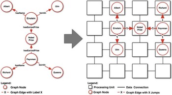
The concept of a Spatially Aware Graph Store is shown in Figure 1. For the sake of simplification, a 2D representation is chosen. However, the presented concept can easily be applied to 1D or 3D physical space. Each square in Figure 1 represents a simple device unit that is capable of storing a single node of the entire graph. All device units are connected by a regular grid structure. In this way, a device unit can communicate directly only with its neighbors. To access nodes stored on non-neighbor device untis, the request needs to be routed over intermediate device units to its destination. Consequently, the delay of a node to access a linked node strongly depends on the distance between these two units. In contrast to this delay, the time to execute an operation on the node stored in a device unit is considered to be negligible. In fact, this assumption can be made as query operations are usually composed of computationally cheap filter operations. Due to the strong dependency of access time on access distance and the ability to process data in one, two or three physical dimensions, the concept resembles a spatial computer.
Example of a graph embedded into a Spatially Aware Graph Store

2.1 Formal structure
The architecture underlying our concept represents an n-dimensional regular grid (cf. Figure 1) of 1D, 2D or 3D. More formally, the grid is represented by a graph G=(V, E) with edge set
 $E\, {\equals}\, \{ \{ (x_{1} ,\,x_{2} ,\ldots\!,\,x_{n} ),\,(y_{1} ,\,y_{2} ,\!\ldots\!,\,y_{n} )\} \,\colon\,\sum_{{i\, {\equals}\, 0}}^{n} \left| {x_{i} {\minus}y_{i} } \right|\, {\equals}\, 1\} $
, and vertex set V={1, 2, …, k}
n
. Moreover, k denotes the number of vertices along 1D of the grid. Hence, the diameter d of the spatial computer is defined by d=nk.
Distances between two nodes (device units) in the grid with integer coordinates (x 1, x 2, …, x n ) and (y 1, y 2, …, y n ) are defined by the Manhattan Distance d(x, y):
 $$d\,(x,\,y)\, {\equals}\, \mathop{\sum}\limits_{i\, {\equals}\, 0}^n \left| {x_{i} \, {\minus} \, y_{i} } \right|$$
Furthermore, the number of neighbors with distance d (x, y)=1 can be controlled by the number of dimensions used. In particular, the number of neighbors is defined as 2n. For example in a 2D grid, each inner device unit can directly communicate with four neighbors, whereas in a 3D grid, this number increases to six units. Therefore, the number of neighbors is defined as 2n.
2.2 Node rearrangement operation
The ability to rearrange nodes presents a basic operation in a Spatially Aware Graph Store. In particular, during the optimization process described in the following Section 3, nodes frequently need to pass through the entire data space of the spatial computer. As there is no central instance to coordinate this movement, a decentralized method is required, which is executed independently on each device unit. Therefore, each device unit can request a swap of its stored data with one of its neighbors. In this way, a graph node can be exchanged between neighbor device units. In particular for each node, the Node Rearrangement Operation consist of four steps:
-
1. Check if the desired position equals the current position, if not proceed to next step.
-
2. Determine all neighbor device units being closer to desired position.
-
3. Request swap with each closer neighbor device unit. If a unit agrees, proceed to next step, otherwise go to step 1.
-
4. Perform swap and go to step 1.
The four steps are repeated, until each graph node has been moved to its desired position. The complexity of this operation depends on the dimensionality of the spatial computer, as the maximum number of swap operations is determined by the diameter of the grid.
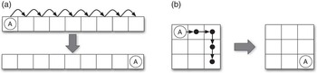
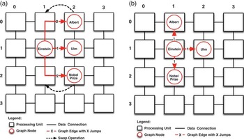
Figure 2 illustrates this case with an example. In a store with nine nodes, node A is linked to other nodes (for the sake of simplicity these links are omitted in Figure 2) in a way that it needs to be moved to the other side of the data space. As the store can only move nodes by local swap operations within its neighborhood, the number of required steps is bound by the dimensionality of the spatial computer. In the example, eight flip operations are needed in a 1D architecture to reach the other side of the data space (Figure 2(a)). However, in a 2D architecture, the number of operations is reduced to four steps (Figure 2(b)). More formally, the complexity of this move operation can be expressed as
 ${\cal O}(n\,{\asterisk}\,\left| V \right|^{{1\!/\,n}} )$
with n being the dimensionality of the spatial computer and |V| being the number of nodes. For example, in a store with 1 000 000 nodes, the worst case number of swap operations is 1 000 000 for a 1D, 2000 for a 2D and 300 for a 3D spatial computer.
Worst case comparison of node rearrangement operation. (a) One-dimensional grid: node A requires eight node swap operations. (b) Two-dimensional grid: node A requires four node swap operations

2.3 Query operation
To achieve efficient query execution on graph data, both primitive operations such as edge traversal as well as filtering need to be executed as fast as possible. Applying a traditional approach where a single coordinator distributes and coordinates all work units is not feasible. This is due to the following two facts. First, the coordination of all participating device units is computationally too expensive for a single device unit. Second, in a spatial computer the access delay depends on the actual physical distance. Consequently, routing all communication to a single device unit results in an unacceptable overhead. Therefore, an execution model is required, which on the one hand reduces the amount of data transferred and on the other hand is independent of a central coordinator. To fulfill these requirements, we suggest to represent each query by a single agent. This model allows the execution of a query to flow along the graph’s edges. Whenever an edge needs to be traversed, the agent is transferred to the destination node’s device unit. Therefore, every filter operation of a node occurs at its device unit, which is a computationally cheap operation. Thus, this execution model fosters the distribution of work among the participating device units and reduces the amount of data to be transferred. More specifically, it prevents long access paths to distant nodes, as all computation is done on the respective device units. However, in spatial computers the time needed to transfer the agent itself cannot be neglected. It is therefore important to reduce the distance between the participating nodes. For the sake of simplicity, we assume that enough space is available on each device unit to handle a certain amount of concurrent queries (e.g. ten query agents). If the number of concurrent queries on the spatial computer exceed a fixed threshold, they are queued and submitted once the previous queries have finished.
3 Linked node distance minimization
In a Spatially Aware Graph Store efficient graph traversal can only be achieved if linked nodes are closely located to each other. To ensure this, a twofold approach is applied. On the one side, the maximum distance between two linked nodes is reduced by increasing the dimensionality of the spatial computer. On the other side, locality is improved by rearranging nodes to reduce the distance to non-neighbor device units.
3.1 Spatial computer dimensionality
As a first step, a graph has to be embedded in the spatial computer (cf. Figure 1). As previously mentioned in Section 2.2, the diameter of the spatial computer and therefore the maximum distance between device units, is reduced with each additional dimension. In this way, the average distance between linked nodes decreases as well.
Consequently, the increase of dimensionality represents a good way to also increase linked node locality. However, only the physical three dimensions can be used for this approach. This poses a problem as graphs are usually high dimensional and therefore no embedding is possible that only consists of edges with length 1. Nevertheless, most real-world graphs are sparse graphs with heterogeneous dimensionality. More specifically, parts of the graph can be 2D, whereas other parts are very high dimensional. This property can be used by a suitable graph embedding to reduce the overall distance between linked nodes. How such an embedding can be obtained is described in the following Section 3.3.
3.2 Graph embedding
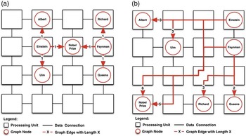
As shown in Figure 1, the embedding of the graph on the device units represents the first step to build a Spatially Aware Graph Store. In the course of this process, many solutions are possible. However, for efficient query processing an embedding mapping from nodes to coordinates of device units is required. In particular, the embedding needs to minimize the Manhattan Distances between linked nodes. Consequently, the costs of an embedding can be measured by its overall sum of Manhattan Distances between linked nodes. Figure 3 shows this with an example graph, which is embedded in two different ways. Although the same graph is embedded, it becomes apparent that solutions can differ significantly in relation to the achievable traversing performance. In more detail, Figure 3(a) shows the optimal solution. The length of each edge is 1, or in other words only one hop is needed to reach its linked node. Therefore, the overall sum of distances is 6 for the entire embedding. In contrast, Figure 6 shows a worse embedding with an overall distance of 22.
Embeddings of the same graph with different overall distances between linked nodes (a) Optimal solution. Overall sum of distances is 6. (b) Worse solution. Overall sum of distances is 22

3.3 Optimization of embeddings
In distributed graph stores, Graph Partitioning (Abou-Rjeili & Karypis, Reference Abou-Rjeili and Karypis2006) is commonly applied to minimize the number of cuts between partitions. However, partitioning does not provide physical locality between partitions when mapped onto the fixed dimensional space of the spatial computer. More specifically, according to our concept, the graph is maximally partitioned already. Each node represents one partition, stored on a single device unit. In this case, a partitioning algorithm cannot improve an embedding any further, as it does not determine how the partitions need to be placed optimally in a spatial computer.
Consequently, this method is unable to increase locality in our environment. However, there is a solution to the problem. Optimal linear arrangement solvers map graphs onto n-dimensional space in a way that the overall sum of edge distances is minimal (Fishburn et al., Reference Fishburn, Tetali and Winkler2000). When applied on a Spatially Aware Graph Store, the distances between linked nodes are minimized and the number of intermediate device units between two linked nodes is reduced (cf. Figure 4).
Mid Point Optimizations example. (a) Non-optimized graph. The overall distance of the embedding is 12. (b) Optimized graph. The overall distance of the embedding is reduced to 5

More formally, the overall sum of distances in the concept can be denoted as costs. The minimization problem (Fishburn et al., Reference Fishburn, Tetali and Winkler2000) of these costs are defined as follows. Given an n-dimensional grid G=(V, E) as defined in Section 2.1 the problem is to find a mapping (permutation) f from V onto {1, 2, …, |V|} that minimizes:
 $${\rm cost}\,{\rm (}G,\,f{\rm )\, {\equals}\, }\mathop{\sum}\limits_{{\rm \{ }i{\rm ,}\,j{\rm \} }{\epsilon}E} {\left( {\left|\, {f{\rm (}i{\rm )}{\minus}f{\rm (}\,j{\rm )}} \right|} \right)} $$
Furthermore, the term (|f(i)−f(j)|) can be replaced by the Manhattan Distance of Equation (2.1) leading to
 $${\rm cost}\,(G,\,d)\, {\equals}\, \mathop{\sum}\limits_{\{ i,j\} {\epsilon}E} {d(i,\,j)} $$
It can be shown that this problem is nondeterministic polynomial time (NP)-hard for directed and undirected graphs (Garey & Johnson, Reference Garey and Johnson1979), which causes the computational requirements to become prohibitive for an optimal solution. However, heuristics can be applied to significantly optimize the node ordering of larger data sets in reasonable processing time (Petit, Reference Petit2003).
3.4 Mid Point Optimization
To approximate the Optimal Linear Arrangement Problem, various different approaches exist. Rodriguez and Tello used Local Optimization and Simulated Annealing (Rodriguez-Tello et al., Reference Rodriguez-Tello, Hao and Torres-Jimenez2008) methods. Also multi-grid approaches have been suggested by Koren and David (Reference Koren and David2002) and Safro et al. (Reference Safro, Ron and Brandt2006) to obtain results of similar costs, but with less processing time. However, for a Spatially Aware Graph Store, two additional issues have to be considered. First, even main memory graph stores are capable of handling up to one billion edges. Therefore, a faster optimization method than Local Optimization and Simulated Annealing is required to achieve better embeddings in feasible time. Second, the method needs to be simple enough to be applicable on each device unit of a spatial computer. This poses a problem for complex algebraic multi-grid approaches.
Therefore, we introduce our novel method called Mid Point Optimization. The basic principle behind this algorithm is to iteratively search for a new embedding with lower costs. This is done by moving a node to the geometrical mean position of all its linked nodes. This position can be calculated, as each node already knows the position of each linked node to process agent-based queries (cf. Section 2.3).
The algorithm is executed on each node of the graph, leading to a new overall node arrangement with reduced costs. In more detail, the method repeatedly executes the following three steps on each device unit:
-
1. Determine the new mid point of the node.
-
2. Perform Node Rearrangement Operation on the node (cf. Section 2.2) to move the node toward the new mid point position.
-
3. Notify all linked nodes of updated position.
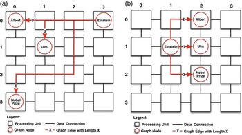
If the new position of a node is already occupied, the swap operation will displace any pre-existing nodes to move the node to its new position. Though this may temporarily destroy good embeddings, the overall result will still improve. This is ensured as the Mid Point operation is constantly executed on all nodes. As a result, in the course of the Mid Point Optimization there is ongoing competition between nodes for the best positions. The algorithm is repeated iteratively until the improvement drops below a predefined threshold. An example of this method is shown in Figure 4. The position of each node is denoted by its 2D coordinates. For example, the node Albert has coordinates (0, 0) and the node Einstein (3, 0). The coordinates are used to calculate the new mid point coordinates. In this process, all results are rounded to the next bigger integer as shown in the following: Einstein ((0, 0)+(1, 1)+(0, 3)+(3, 0))/4=(1, 1), Ulm ((1, 1)+(3, 0))/2=(2, 1), Nobel Prize ((0, 3)+(3, 0))/2=(2, 2) and Albert ((0, 0)+(3, 0))/2=(0, 2). Figure 4(b) shows the resulting embedding. It can be seen from the preceding example that the initial embedding with an overall distance of 12 (cf. Figure 4(a)) can be optimized to an embedding with overall distance of 5 (cf. Figure 4(b)).
3.5 Local Node Optimization
The Mid Point Optimization efficiently moves nodes over long distances through the data space. In this way, it can optimize nodes that are located far away from their optimal position. However, the resulting embedding can still be considered as a rough solution, which can be further improved through another finer grained method. For this purpose, we suggest the Local Node Optimization. The basic principle behind this algorithm is to search new embeddings with strictly shorter distances. In more detail, the following three steps are repeatedly executed on each device unit:
-
1. Determine if a swap of nodes with a neighbor device unit decreases distances to linked nodes. If true, proceed to next step, otherwise end execution.
-
2. Perform a Node Rearrangement Operation with the neighbor device unit (cf. Section 2.2). This results in a swap of the two nodes.
-
3. Notify all linked nodes of updated position.
Figure 5 shows an example of the Local Node Optimization. As a starting point, the optimized embedding after the Mid Point Optimization is used (cf. Figures 4(b) and 5(a)). Further applications of the Mid Point Optimization do not lead to a better embedding, whereas the Local Node Optimization is able to find a better solution. In particular, the nodes Einstein and Ulm cannot be swapped without causing higher distances. However, the nodes Albert and Nobel Prize can both be swapped with their left neighbor. This reduces the overall distance of the embedding to 3. In fact, this is the global minimum for this graph. Obviously, for larger graphs the calculation of the global minimum is not feasible as the exact solution remains NP-Hard. Nevertheless, the example shows how the Local Node Optimization is able to improve existing embeddings gained by the Mid Point Optimization.
The Local Node Optimization applied on the result of the Mid Point Optimization. (a) Embedding after Mid Point Optimization. The overall distance of the embedding is 5. (b) After Local Node Optimization. The overall distance of the embedding is reduced to 3

In traditional non-spatial computing environments, local optimization methods have two major drawbacks. First of all, local optimization does not scale well in the 1D case. Similar to the previously discussed node rearrangement operation in Section 2.2, the reason for this is the large number of swap operations that are required. In particular, the diameter in a 1D spatial computer is orders of magnitudes higher than in the 2D or 3D case. Thus, the required number of steps of the Local Node Optimization increase at the same rate, which makes this method unfeasible for larger graphs. Second, the Local Node Optimization relies on a strict improvement of the next result and is therefore vulnerable to local minima. Stochastic methods like Simulated Annealing (Rodriguez-Tello et al., Reference Rodriguez-Tello, Hao and Torres-Jimenez2008) are able to overcome such situations by adding artificial noise to the system. However, these methods are computationally too expensive for large real-world data sets. Yet, in a Spatially Aware Graph Store the effect of these issues can be relaxed. First, in 2D and 3D spatial computer the worst case number of swap operations decreases significantly, as it has already been shown for the Node Rearrangement Operation. The same effect results in a speed-up for the Local Node Optimization in 2D and 3D environments. Furthermore, we use the Local Node Optimization only to refine the result of a Mid Point Optimization. In this way, nodes are already placed at roughly optimal positions. In this case, the Local Optimization require only a limited number of swaps to find better embeddings. Second, the probability of local minima is reduced in higher 2D or 3D spatial computers as there are more possibilities to escape through the additional dimensions.
Despite the improvement that is gained through the Local Optimization, nodes with many edges present a problem for both optimization methods. Therefore, the next section deals with this issue in more detail.
3.6 Large Node Decomposition
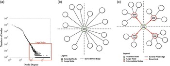
Many graph data sets represent scale free graphs. In this class of graph data, the distribution of node degrees follows power law. In other words, the majority of nodes are connected only to a few other nodes. Nevertheless, there are hub-like nodes as well, which link to a significant amount of nodes of the entire graph. The histogram shown in Figure 6(a) shows an example of a scale free graph data set. The x-axis in this histogram indicates the node degree and the y-axis the frequency of nodes with that degree. Both axis are scaled logarithmically. Despite most of the nodes are having a low node degree (left side of the histogram), it becomes apparent that a few nodes with very high degrees exist (right side of the histogram). In the following, we denote these hub nodes as large nodes.
Overview of Large Node Decomposition. (a) Frequencies of node degrees in a scale free graph. The red box marks large nodes that need to be decomposed. (b) Before node decomposition. All nodes of Nobel Prize winning scientists are attached to one large Nobel Prize node. (c) After node decomposition. The Nobel Prize node was split into five nodes. The original node and a new node for each quadrant

In Spatially Aware Graph Stores large nodes cause two major problems. First, the runtime of many graph operations on a single node depends to a large extent on its number of edges. As all device units of the spatial computer have the same CPU performance, this leads to bad concurrency. In particular, large nodes consume significantly more processing time than the majority of the other nodes with less edges. Therefore, these nodes represent a bottleneck during graph processing.
Second, the distances between a large node and its linked nodes can be minimized only to a certain extent. For example, a node that is connected to almost all other existing nodes is placed optimally in the middle of the data space. In this way, the distances to all linked nodes is minimized. An example of such a solution is shown in Figure 6(b). However, the average linked node distance remains a quarter of the maximal distance. To resolve these two issues, we introduce the Large Node Decomposition method. The general idea behind this method is to recursively split large nodes, until their degree is below a predefined threshold. In more detail, the method executes the following five steps on each device unit (cf. Figure 6):
-
1. If the stored node has a larger degree than the predefined threshold (green node) proceed to the next step.
-
2. Create four new intermediate nodes, each for one quadrant.
-
3. Move all edges of a quadrant from the large node to the corresponding intermediate node.
-
4. Add a downlink from the large node to the new intermediate node.
-
5. Migrate the new intermediate nodes to their mid points using the Mid Point Optimization as described in Section 3.4.
The method naturally operates in recursive manner until all nodes meet the predefined threshold. After the application of the Node Decomposition large nodes have been split up into smaller, hierarchically linked nodes. However, all other nodes need to be optimized again to react on their changed linked nodes. Consequently, a Local Node Optimization is subsequently executed on the entire graph. This results in a new graph embedding with decomposed nodes and shorter distances between linked nodes.
It is important to note that the previously described algorithm needs to be executed on an already optimized embedding. In this way, the position of each node is stable and unlikely to change the quadrant in the subsequently executed Local Node Optimization. If this is not the case, nodes will be linked to intermediate nodes of the wrong quadrant, which leads to higher distances. Hence, we apply the Node Decomposition method on already fully optimized data sets using the Mid Point and Local Node Optimization.
3.7 Summary
To realize efficient querying in Spatially Aware Graph Stores, the minimization of distances between linked nodes is of particular importance. In this section, four methods that minimize these distances have been presented. First, the dimensionality of the spatial computer is increased to reduce distances. In this way, the physical second and third dimensions are used to embed graph data with reduced distances. However, graph data has usually more than three dimensions. Therefore, the Mid Point and Local Node Optimization have been presented as a second and third step. Both methods reduce distances by iteratively rearranging nodes to discover better embeddings. In the final step, we addressed the problem of large nodes, which appear in scale free graphs. These nodes have a negative effect on concurrency and distance optimization. Consequently, we introduced the Large Node Decomposition method, which recursively splits large nodes, to further improve node embeddings. The performance of each presented method is evaluated in the subsequent Section 4.
4 Evaluation
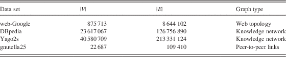
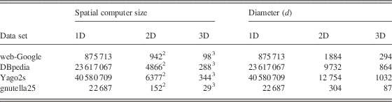
To evaluate our concept of a Spatially Aware Graph Store we conducted three experiments. First, we surveyed the influence of 2D and 3D storage of graph data on edge length. Second, the decrease of edge length by subsequently applying the Mid Point and Local Node Optimization and the Large Node Decomposition method is evaluated. Finally, the effects of optimization on query execution is examined. The evaluation is carried out on the following four real-world data sets web-GoogleFootnote 2 , gnutella252, DBpediaFootnote 3 and Yago2sFootnote 4 . These data sets were selected to provide a balanced overview on optimization results in the best (web-Google), average (DBpedia, YAGO2s) and worst case (gnutella25). Table 1 shows the details on the evaluated data sets and Table 2 presents the size and diameter of the used spatial computers instances.
The evaluated data sets

Sizes and diameters of the spatial computers

1D=one dimensional; 2D=two-dimensional; 3D=three-dimensional.
To the best of our knowledge, no hardware exists on which a Spatially Aware Graph Store could be evaluated. Therefore, we implemented a simulation engine of a Spatially Aware Graph Store, which is able to load, optimize and query data sets. To evaluate the required number of steps of our proposed optimization methods, we decided to execute the simulation engine in a synchronous manner. In particular, the execution is separated in a number of iterations in which each device unit is executed once. This approach allows to determine when an optimization method has reached a minimum and how many steps were needed.
4.1 Two and three-dimensional embeddings
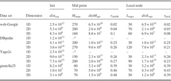
In the first experiment, each data set was loaded into the Spatially Aware Graph Store in a 1D, 2D and a 3D embedding. To avoid any pre-existing locality, the nodes of each data set were inserted in random order. The column dist org in Table 3 contains the sum of all distances between linked nodes after this insertion process. It can be observed that in the 2D case, the distances between linked nodes are reduced by two to three orders of magnitude in comparison to the 1D case (e.g. the web-Google data set improves from 2.5×10¹² to 5.3×10⁹). Furthermore, the 3D case improves by another order compared with the 2D case (the web-Google data set improves from 5.3×10⁹ to 8.3×10⁸). It can be inferred that by embedding a graph in a higher dimensional spatial computer, distances between linked nodes are significantly reduced.
Reduction of distances to linked nodes in a one-dimensional (1D), two-dimensional (2D) and three-dimensional (3D) Spatially Aware Graph Stores by the Mid Point and Local Node Optimization

aSkipped after 72 hours.
4.2 Mid point iteration
The second experiment executes the Mid Point Optimization on each data set in the 1D, 2D and 3D case. The optimization is aborted after the overall improvement of a single execution step drops below 1%. In addition, the abort condition is reevaluated after each 10th step. The resulting distances between linked nodes after this optimization can be found in Table 3 in column distM opt. In addition, the ratio between distM opt and dist org is labeled as r distM. As a result, distances were reduced by a factor 0.02 to 0.48 in relation to the original costs (cf. web-Google with r distM=0.04 for the 2D and 0.1 for the 3D case). The required number of iterations for the method is denoted in the Table 3 as M steps.
Another important point is that the number of steps (iterations) increases sub-linearly in relation to the size of the data set. For example the Yago2s data set consist of >20 times more edges than the web-Google data set (cf. the |E| values in Table 1). However, the Mid Point Optimization is able to optimize both data sets within 300 steps (cf. Table 3 M steps<300).
4.3 Local optimization
In a next step, the improvement of distances between linked nodes by applying the Local Node Optimization has been evaluated. As initial data we used the 2D and 3D embeddings, which were created through the application of the Mid Point Optimization. In addition, the same termination condition as for the Mid Point Optimization has been used. Consequently, the optimization has been terminated as soon as the overall improvement of a single execution step drops below 1%.
The results of the Local Optimization can be found in column distL opt in Table 3. The column r distL contains the ratio between distL opt and dist org. It can be seen that no significant improvements could be achieved in the 1D and 2D cases. More specifically, in these cases the execution costs of the Local Optimization outweighs the improvements. In the best 2D case, the gnutella25 could be improved by about 15% (r distL=0.43 and r distM=0.5). In the worst 2D case (DBpedia), no improvement could be achieved at all. However, in 3D case all data sets could be markedly improved. The relative improvement compared with the result of the Mid Point Optimization ranges from 20% (web-Google) to 15% (Yago2s). The L steps value in Table 3 describes the number of required steps of the Local Node Optimization to reach the minimum. For example, in the 3D case of the DBpedia data set, 120 steps were executed until the overall improvement dropped below the 1% threshold (Figure 7).
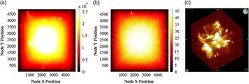
The DBpedia data set stored in a two-dimensional (2D) and three-dimensional spatially aware graph store. (a) 2D: edge density before optimization. (b) edge density map of query DBpediaQ1 before optimization. (c) 3D: edge density after optimization

4.4 Large node decomposition
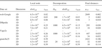
Analogous to the previous step, the Large Node Decomposition was evaluated by applying the method on the results of the previous Local Optimization method in two and three dimensions. The results of this experiment can be seen in column distD opt. The ratio to the original embedding dist org is denoted as r distD. The used node decomposition thresholds D thr for each data set are shown in Table 4.
Reduction of distances to linked nodes in one-dimensional (1D), two-dimensional (2D) and three-dimensional (3D) Spatially Aware Graph Store by the Local Node Optimization and Large Node Decomposition

aSkipped after 72 hours.
In comparison to the Local Optimization the Large Node Decomposition results in significantly improved embeddings. With the exception of the gnutella25 data set a further improvement by 40% could be achieved (cf. DBpedia data set for the 2D case with r distL=0.25 and r distD=0.15). The reason why the achieved improvement of the gnutella25 is below 1% is that the gnutella25 data set is not scale free. It can be observed, when comparing the Node Distribution Plots of the gnutella25 (cf. Figure 10(c)) and the Yago2s (cf. Figure 11(c)) data set, that the amount of large nodes, which can be processed by the Node Decomposition algorithm is higher in scale free data sets.
The last two columns of Table 4 show the final distances after all three optimization methods have been applied. In particular, μ 1/2 shows the median distance between two linked nodes and r max denotes the ratio between μ 1/2 and the diameter d of the spatial computer (cf. Table 2). For example, in the 3D web-Google case r max=0.010. This means, on an average, each node needs to cross 1/100 of the entire spatial computer to reach a linked node.
4.5 Detailed results visualization
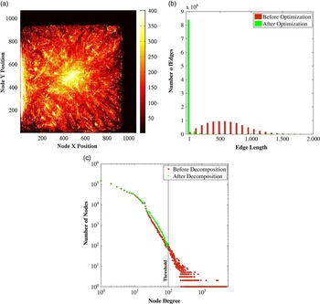
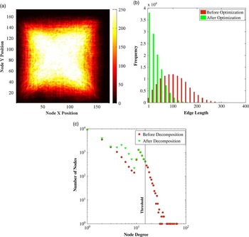
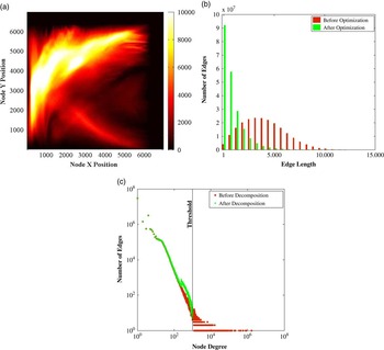
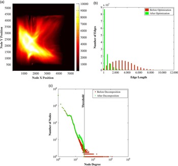
The detailed results of the optimization are visualized in Figures 9–12 as Edge Density, Edge Length Histograms and Node Distribution Plots. Edge Density Plots (on the top) are heat maps created by counting the number of edges crossing a location in the data space. In particular, dark colors denote few edge crossings and brighter colors denote frequent edge crossings. For instance, the color white in Figure 11(a) denotes >10 000 edge crossings at a single position.
Edge Length Histograms (plots in the middle) visualize the distribution of edges according to their length. Red bars represent the distribution of edges before the optimization process and green bars the resulting distribution after the optimization.
The Node Distribution (plots on the bottom) is a double logarithmic dot plot, which visualizes the distribution of nodes according to their node degree. Red dots represent the node distribution before and green triangles the result after Node Decomposition. In addition, the threshold D thr (cf. Table 4) is marked in the plots. Due to limited illustration facilities, only the results of the 2D embeddings are visualized in this paper. However, the DBpedia 3D Edge Density Plot is shown in Figure 7(c) as an example. For all other plots, we provide an online supplementary materials sectionFootnote 5 .
For each data set, all three visualizations are stacked on top of each other. The Edge Density Plot presents the Edge Densities after the Optimization. The original Edge Density Plot before optimization conforms to a random distribution for each evaluated data set. Therefore, we decided to present only the Edge Density Plot of the DBpedia data set in Figure 7(a) as a representative for all data sets.
By comparing the Edge Density Plots of each data set, the difference between best and worst case optimization results becomes visible. In particular, it becomes apparent that the best case web-Google data set is effectively clustered into weak connected parts. As a consequence, edge length are reduced significantly. For the average cases (Yago2s and DBpedia), large areas of the data sets show weakly connected nodes. However, both data sets contain highly connected clusters, which cannot be further optimized in 2D space. Finally, the gnutella25 data set represents the worst case of a highly random connected graph. In this case, no weakly connected parts exist that can be used to calculate an improved embedding.
The different optimization ratios (cf. Column r distD of Table 3) can be observed in the Edge Length Histograms as well. Figure 9(b) shows this for the web-Google data set. In the best case, edge lengths are significantly reduced, which is represented by the long green bar at the very left of the diagram. In the average and worst case, longer edges appear in the diagrams, indicating an embedding of lower costs.
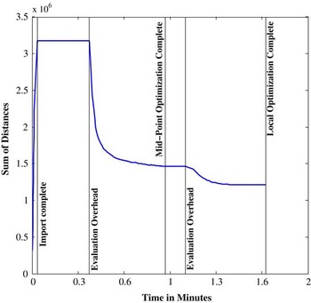
The development of distances during optimization is another interesting point. Figure 8 shows more details on this with a distance development plot of the gnutella25 data set. On the x-axis the time in minutes and on the y-axis the corresponding sum of distances at this point of time is visualized. It becomes apparent that the Mid Point Optimization quickly decreases distances until it reaches a preliminary minimum. At this point, the Local Node Optimization is applied to further improve the result. During the flat segments marked by evaluation overhead no optimization has been executed but evaluation data has been calculated and stored. In a real-world implementation, these segments would disappear.
The development of the sum of all distances for the gnutella25 data set in a three-dimensional Spatially Aware Graph Store. The result converges to a minimum

Finally, the Node Distribution Plots show the effect of the Node Decomposition method on each data set. In all data sets, nodes larger than the predefined threshold are successfully split into smaller nodes. This can be observed by the lack of green triangles on the right side and by green triangles with higher frequencies on the left side of the threshold mark.
In the last experiment, the impact of the optimization methods on the agent-based query engine is evaluated.
4.6 Queries
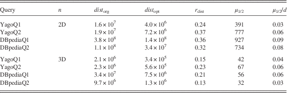
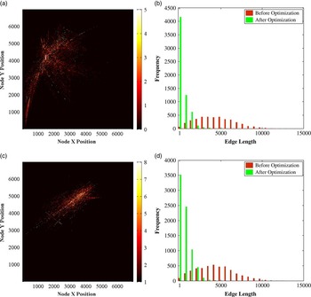
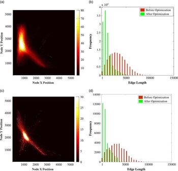
The results of Table 3 indicate a significant reduction of edge lengths in the entire data set. However, an actual query agent will only access a limited part of the data set. In addition, highly connected areas (bright areas in the Edge Density Plots) are more likely to be visited. In these areas, the distances between nodes are above average. To get more insights on the impact of this effect, two queries on each of the data sets Yago2s and DBpedia have been evaluated. To execute the queries, the agent-based approach as presented in Section 2.3 has been used. The details on this queries are presented in the Listings 1–4.
The results of this experiment are shown in Table 5 for the 2D and 3D case. In more detail, the column dist org shows the aggregated distances a query traversed in the unoptimized and column dist opt in the optimized case. The column r dist denotes the ratio between these two values. It becomes apparent that though the queries are executed in dense areas, an average distance reduction by the factor 0.3 is achieved in the 2D case. In addition, the last two columns describe the median μ 1/2 distance to linked nodes and μ 1/2/d denotes the ratio between this distance and the spatial computer diameter d (cf. Table 2). For example, the median distance for the YagoQ1 query is 42 device units, which corresponds to 4% of the spatial computer diameter. More details on the specific queries are shown in Figure 13 for the Yago2s and in Figure 14 for the DBpedia data set, respectively. For each query, the Edge Density Plot and the Edge Length Histogram is shown. The former visualizes the part of the spatial computer which has been accessed by the specific query. By comparing the Edge Density Plots of a specific query with the corresponding Edge Density Plot of the entire data set, it becomes apparent that large portions of the query accesses highly connected areas (cf. Figures 13(a) and 11(a)).
Reduction of distances to linked nodes for queries executed in two-dimensional and three-dimensional Spatially Aware Graph Stores

For the unoptimized case, the Edge Density Plots of each query show similar random distributions. Therefore, we only present the Edge Density Plot of the YagoQ1 query in Figure 7(b). It becomes clear, that in the unoptimized case, the nodes accessed by the query agent are randomly scattered over the entire data space. However, in the optimized embedding the participating nodes are closely located. As a consequence, the query accesses only parts of the data space (Figures 9–12).
Results of web-Google data set. (a) Edge Density Map after optimization. (b) Edge Length Histogram. (c) Node Degree Distribution

Results of gnutella25 data set. (a) Edge Density Map after Optimization. (b) Edge Length Histogram. (c) Node Degree Distribution

Results of Yago2s data set. (a) Edge Density Map after optimization. (b) Edge Length Histogram. (c) Node Degree Distribution

Results of DBpedia data set. (a) Edge Density Map after optimization. (b) Edge Length Histogram. (c) Node Degree Distribution

Listing 1: YagoQ1: all data of Canada’s Provinces.
Listing 2: YagoQ2: all locations in Vienna, which are related to the Viennese Actionism.
Listing 3: DBpediaQ1: unconstrained query for artworks, artists, museums and their directors.
Listing 4: DBpediaQ2: two degrees of separation from Kevin Bacon.
The same effect can be observed in the Edge Length Histograms as well. In particular, the random access pattern visualized by the red bars resembles a Gaussian distribution. On the contrary in the optimized case, which is represented by the green bars, short edge lengths are dominating (cf. Figure 13(b). Finally, for the 3D spatial computer an average distance reduction by the factor 0.18 is achieved. The improved results in relation to the 2D cases can be explained by the better performance of the Local Node Optimization in the 3D data space. In particular, the distance reduction that could be achieved through the Local Node Optimization is also reflected on the query performance (cf. Section 4.3).
Yago2s query evaluation results. (a) YagoQ1: Edge Density Map after optimization. (b) YagoQ1: Edge Length Histogram. (c) YagoQ2: Edge Density Map after optimization. (d) YagoQ2: Edge Length Histogram

4.7 Simulation times
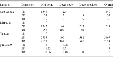
Table 6 shows the required times in minutes to optimize the data sets with the suggested methods Mid Point, Local Node and Large Node Decomposition. For the Mid Point Optimization, it becomes apparent that the simulation time can be significantly reduced with a higher dimensional spatial computer. For example the Mid Point Optimization requires 1348 minutes to reach a minimum for the web-Google data set in the 1D case. However, the required runtime drops to 24 minutes for the 2D and to 15 minutes for the 3D case. This effect is caused by the lower diameter of 2D and 3D Spatially Aware Graph Stores. In particular, less swap operations are needed to move nodes to their mid point positions.
Simulation times of all methods in one-dimensional, two-dimensional and three-dimensional Spatially Aware Graph Stores

All times are in minutes.
aSkipped after 72 hours.
The Local Node Optimization shows the opposite behavior, as with more dimensions its runtime increases. For example, the DBpedia data set takes 68 minutes in a 2D and 307 minutes in a 3D Spatially Aware Graph Store to be optimized. This can be explained as in the 2D and 3D case more steps are executed as well (cf. L steps in Table 3). Moreover, the number of neighbors to check increases from two in the 1D to four in the 2D and six in the 3D case (Figure 14).
DBpedia query evaluation results. (a) DBpediaQ1: Edge Density Map after optimization. (b) DBpediaQ1: Edge Length Histogram. (c) DBpediaQ2: Edge Density Map after optimization. (d) DBpediaQ2: Edge Length Histogram

The Decomposition column shows the simulation times of the Large Node Decomposition method. Similar to the Mid Point Optimization, less time is required in the 3D case than in the 2D case. Again, the grid diameter is the reason for this speed-up as the new intermediate nodes (cf. Section 3.6) need to move less to their corresponding mid point positions.
Finally, the last column shows the required simulation time for the overall procedure. It becomes apparent that the largest data set Yago2s with 213 331 124 edges can be optimized in ~2 days (2954 minutes). This corresponds to about 1203 edges per second for an average case data set.
4.8 Discussion
In this section the performance of the suggested methods Mid Point and Local Node optimization and Large Node Decomposition has been evaluated. As result of the evaluation, it becomes apparent that all three optimization methods are able to reduce the distance between linked nodes significantly. This could be shown for entire data sets as well as with sample queries executed in highly linked areas.
The Mid Point Optimization is the most important of all three methods. It is able to reduce distance even in large real-world data sets as it quickly converges toward a minimum. Despite of its performance, its vulnerability to local minima seems to be low as we could achieve good results in all four data sets.
On the contrary, the benefit of the Local Node method to refine the result of the Mid Point method is arguable. In most 1D and 2D cases none or a very limited reduction of distance could be observed. The reason for this lies in the high vulnerability to local minima of the method. This also becomes apparent as the performance improves for the 3D case. In case of 2D or 3D spatial computers, we identify two properties that support the Local Node optimization. First, more neighbors can be used to escape a local minima and second the ratio between the size of the neighborhood (Manhattan Distance 1 in this work) to the overall size of the spatial computer increases. The latter is important as, for example, in the 3D case, the distance reduction per step is more significant as in 1D or 2D. As a consequence, the Local Node Optimization seems to be only useful in 3D Spatial Aware Graph Stores.
The Large Node Decomposition is able to reduce distance for scale free data sets (web-Google, DBpedia and Yago2s). Despite its lower performance compared with the Mid Point Optimization, there are two reasons to use this method for Spatially Aware Graph Stores. First scale free data sets are very common and therefore the evaluated benefits will apply on many real-world data sets. Second, nodes with a very high degree require more resources to process as the complexity of most data store operations (e.g. querying) depend on the number of edges not on the number of nodes. Splitting large nodes into several smaller nodes therefore enables a better distribution as more device units manage a single large node. As a consequence, the Large Node Decomposition does not only reduce the distance between linked nodes, but will also improve load balancing in future works.
An important question arises to what extent the suggested methods depend on local or global data. As global data access is expensive in spatial computers all proposed methods are simple methods, which are able to work on local data. However, in all three methods linked nodes have to be notified if a node moves using the node rearrangement operation. As all nodes are able to move concurrently, this is not a trivial problem. In particular, a position update is hard to deliver as linked nodes might also have changed their position. A local solution to this issue is possible by using a breadcrumbs approach. On each swap operation, a node stores its new position at the preceding device unit. If another node sends a position update, it will start at the old position of the destination node and follow the breadcrumbs until it reaches the desired node. This approach works efficiently in a spatial computing environment as only local data are required. In this work however, we are mainly interested in the effect of the suggested optimization methods. Therefore, we use a global lookup table in the simulation engine.
As explained at the beginning of Section 4, we used a synchronized simulation engine to evaluate our methods. This allows us to use thresholds to detect when an optimization process should be terminated. In addition with this approach, the number of required steps toward the minimum can be counted. However, spatial computers use asynchronous execution, which makes the use of thresholds expensive as global data access is required. Nevertheless, all suggested methods are able to run in an asynchronous environment as well. For example, a Spatially Aware Graph Store is feasible that constantly applies the Mid Point Optimization to reduce distances to linked nodes. In this case, no threshold is required and the optimization process would run forever.
5 Related work
To the best of our knowledge, there are only the works of Delorimier and Kapre (Reference Delorimier and Kapre2006) and Delorimier et al. (2011) that followed a similar approach to combine the concept of spatial computers with Graph-Based Processing. These works resulted in the GraphStep system, a novel FPGAs-based graph processing model. However, our work differs significantly from their approach and focuses on a specialized concept for graph stores instead of a general compute model. In addition, the optimization of access times using optimal linear arrangement solvers presents an important cornerstone of this work, which has not been discussed by Delorimier et al. Furthermore our approach simulates a 1D, 2D and 3D spatial computer and is therefore not restricted to the 2D FPGA design.
In the area of non-spatial computers, several approaches for graph stores exist. At the beginning, general frameworks which were able to map resource description framework (RDF) data onto different existing databases were developed (Broekstra et al., Reference Broekstra, Kampman and van Harmelen2002; Wilkinson et al., 2003). Although they supported a flexible interface and architecture in terms of performance, they were soon rendered obsolete by the design of dedicated graph stores. These dedicated graph stores can be separated into two categories. On the one hand, we denote optimized relational triple-based stores (Abadi et al., 2007; Neumann & Weikum, Reference Neumann and Weikum2008; Erling & Mikhailov Reference Erling and Mikhailov2009) as Join Based. On the other hand, we denote main memory stores (Janik & Kochut, Reference Janik and Kochut2005; Binna et al., 2010; Shao et al., Reference Shao, Wang and Li2012) as Graph Exploration Based. Although providing sufficient performance, these dedicated stores were restricted to a single machine. To cope with larger linked data sets, new approaches were developed to distribute stores onto several hosts.
To distribute Join Based stores approaches based on existing distributed databases, the Map Reduce paradigm (Huang et al., Reference Huang, Abadi and Ren2011; Husain & McGlothlin, Reference Husain and McGlothlin2011) or custom distribution architectures (Erling, Reference Erling2008; Harris et al., Reference Harris, Lamb and Shadbolt2009) exist. The approaches by Erling (Reference Erling2008), Harris et al. (Reference Harris, Lamb and Shadbolt2009) and Harth et al. (2007) primarily use hash-based partitioning to distribute the triples according to the subject node. To reduce the number of edges between different hosts Huang et al. (Reference Huang, Abadi and Ren2011) use partitioning, whereas Husain and McGlothlin (Reference Husain and McGlothlin2011) use the Hadoop HDFS filesystem (Shvachko & Kuang, Reference Shvachko and Kuang2010) to distribute their data. Regarding the query execution, these Join Based stores use distributed join operations.
In the case of Graph Exploration Based stores, Zeng et al. (2013) invented the Trinity.RDF system, which is able to scale to several nodes. This system is based on the Trinity key-value store created by Shao et al. (Reference Shao, Wang and Li2012), which is inspired by the RAM-Cloud concept of Ousterhout et al. (2011). Furthermore, a similar system was presented by Mondal and Deshpande (Reference Mondal and Deshpande2012).
First in-depth experiments on the Minimum Linear Arrangement (MinLA), also known as Optimal Linear Arrangement problem, were conducted by Petit (Reference Petit2003). Simulated Annealing is the most traditional approach to optimize data sets, which leads to good results as it successfully escapes local minima (Johnson et al., 1989). However, this method features nonlinear runtime complexity and therefore cannot be applied on large-scale data sets (Rodriguez-Tello et al., Reference Rodriguez-Tello, Hao and Torres-Jimenez2006; Rodriguez-Tello et al., Reference Rodriguez-Tello, Hao and Torres-Jimenez2008). Consequently, faster concepts using multi-grid techniques (Brandt et al., Reference Brandt, Ron and Amit1986) became more popular. Koren and David (Reference Koren and David2002) and Safro et al. (Reference Safro, Ron and Brandt2006) presented such multi-grid algorithms to solve the MinLA problem. Additional vertex ordering problems are presented by Safro et al. (Reference Safro, Ron and Brandt2009).
Furthermore, Graph Visualization algorithms (Walshaw, Reference Walshaw2003; Harel & Koren, Reference Harel and Koren2004; Hu, Reference Hu2006) are related to the MinLA problem as their objective is to minimize edge lengths between linked nodes in 2D space. However, the problem behind graph visualization is much broader than MinLA, as it needs to consider the full range of human perception characteristics to achieve good results. For instance, Nguyen et al. (2011) showed that crossing angles between edges need to be considered to improve human readability.
6 Conclusion and future work
This work introduced a novel concept of Spatially Aware Graph Stores to address contemporary memory wall and scalability issues. It has been shown that the combination of a Graph Store and a spatial computer represents a way to enhance existing architectures by taking advantage of storing information in one, two or three physical dimensions. Furthermore, a realization of the concept needs to locate nodes as close to their linked nodes as possible to enable efficient graph traversal. Consequently in this work, the distance between linked nodes has been minimized with a twofold approach. First, the effect of increasing the dimensionality of the Spatially Aware Graph Store on the overall distances between linked nodes has been evaluated. In fact, 2D and 3D Spatially Aware Stores reduce these distances by up to three orders of magnitude in comparison with a 1D realization. Second, we have shown that the Mid Point and Local Node Optimization methods are able to further decrease distances between linked nodes by another order of magnitude. Furthermore, an additional reduction of edge length can be achieved by the Large Node Decomposition method for scale free graphs. Finally, the results on querying the DBpedia and Yago2s knowledge networks showed comparable improvements, as on optimized data sets query agents need to travel significantly less through the spatial computer.
We conclude that our concept of a Spatially Aware Graph Store in combination with optimization algorithms provides a sound basis for efficient graph stores that are less vulnerable to the memory wall issue and enable distribution on a massive scale. In future work, many challenging issues have to be addressed to further develop the concept. The next steps will be to refine the Large Node Decomposition method to further improve embeddings. In addition, the application of a weighted graph model represents an interesting opportunity to optimize frequently queried areas.
Finally, a practical realization of the proposed system is an important point. Though there is no common hardware consisting of millions of device units, a prototype with less device units seems feasible. Possible realizations are presented in the work of Butera (Reference Butera2002), who suggested a reference architecture based on microprocessors for his Paintable Computer. In addition, Delorimier et al. (2011) used FPGAs to realize a spatial computer. In the course of a realization, we however need to consider that real-world data sets require a lot of storage space and that the number of device units will become smaller in relation to the number of nodes. Therefore, the storage of more than one node on a single device unit seems inevitable for future approaches.
Acknowledgments
Dominic Pacher was supported by a scholarship from the University of Innsbruck (Doktoratsstipendium aus der Nachwuchsförderung, MIP8/2012/1).
Supplementary Material
To view supplementary material for this article, please visit https://doi.org/10.1017/S0269888916000187