The power to remove the government via no-confidence motion (NCM) is a powerful tool afforded to the parliament to hold the government accountable. Needless to say, when successful, NCMs have substantial impacts on policy direction in parliamentary democracies. For instance, the successful NCM against James Callaghan’s minority Labour government shepherded in an era of Conservatism under Margaret Thatcher. Likewise, the Japanese opposition used an NCM in 1993 to remove the Liberal Democratic Party (LDP) from power for the first time since 1955. These rare cases, however, are in stark contrast to the vast majority of NCMs that fail to muster a parliamentary majority, and thus represent little threat of taking down the government. Under what circumstances do opposition parties utilize this tool? Moreover, what factors determine the motion’s likelihood of passage?
The first step in answering these two questions is to realize that they are not distinct, but instead are inseparable on account of being products of a series of interactions between parties. First, consider the decision by an opposition party to propose an NCM. If the opposition party intends to remove the government then it will carefully calculate its chance of success based on the anticipated reactions of others. Second, whether or not the NCM is successful is not an isolated outcome, but is the result of strategic planning by those who proposed the motion and those in parliament who might benefit from its passage. As these two questions are grounded in strategic decisions, empirical examinations must carefully model these interdependent actions.
Unfortunately, the current literature examining the relationship between opposition behavior and government stability based on formal and empirical models cannot effectively answer these questions. Our understanding of NCMs is primarily driven by formal models of parliamentary dynamics that highlight their key role in the formation (e.g., Baron Reference Baron1991), stability (e.g., Austen-Smith and Banks Reference Austen-Smith and Banks1990), and termination of government (e.g., Baron Reference Baron1998). In these models, opposition parties use NCMs to remove the government (e.g., Lupia and Strom Reference Lupia and Strom1995; Diermeier and Stevenson Reference Diermeier and Stevenson1999; Diermeier and Stevenson Reference Diermeier and Stevenson2000). In this line of reasoning, we should expect to see a high percentage of NCMs actually gain majority support and lead to the termination of government. Yet, the empirical record suggests otherwise. In fact, in a sample of 19 parliamentary democracies from the late-1950s–2006 I find that only about 4.3 percent of NCMs are passed by parliament. This low success rate is not surprising, however, when one considers that a secondary motivation of opposition parties is to propose NCMs to improve their electoral prospects (Williams Reference Williams2011; Williams Reference Williams2014). The NCMs act as signals of the opposition party’s abilities to govern vis-à-vis the current government, which voters use when deciding which party to support.
Empirical studies of government termination, on the other hand, tend to identify the factors that influence the second question posed above (i.e., government survival), without realizing that stability is the end result of a series of strategic decisions taken by multiple actors. Failing to properly model the first step (i.e., the decision to propose an NCM) distorts the strategic nature of the model and ignores the possibility that key variables (such as government tenure or the election cycle) may have different effects at various stages of the process.
I develop a formal model of this strategic decision-making process that identifies the factors influencing the occurrence and success of NCMs. I theorize that opposition parties carefully weigh the likelihood of being in the next post-election government against its value from the current governing arrangement and the costs that accompany proposing the NCM. Likewise, the median legislator—as the decisive actor in parliament—faces a decision where she weights her value from the current governing arrangement against the possibility of being in the next government. I test these expectations via statistical backwards induction (SBI), which properly takes into account the strategic considerations that guide the decisions by both actors. I find that the likelihood of an NCM (as well as its success rate) increases as the next constitutionally mandated election approaches. At the same time, older governments tend to deter challenges because they are more stable. NCMs have the highest chance of success when they are targeted at minority parties in systems where there is a strong possibility that the median legislator in parliament is returned to office.
This study offers a series of implications about parliamentary decision making. First, this project is unique in providing an empirical test of government termination in a manner that models sequential decisions by important actors. Second, this study is the first of its kind to develop a theory of opposition party behavior and then empirically test those expectations in a cross-national fashion. The empirical results warrant a reconsideration of the conventional wisdom that NCMs are solely motivated by bringing down the government. I provide evidence that opposition parties propose NCMs at strategically opportunistic situations when they can benefit electorally. Third, the different motivations that opposition parties possess means that their behavior varies as a function of government tenure and the election cycle. Opposition parties respond differently to changing incentives as governments age and the next election approaches, ceteris paribus, which can produce wildly different behaviors. These contrasting effects shed light on the debate about rising hazards of government termination (e.g., Warwick Reference Warwick1992; Lupia and Strom Reference Lupia and Strom1995; Diermeier and Stevenson Reference Diermeier and Stevenson2000). Finally, I offer an explanation for the extremely low success rate of NCMs. For an NCM to pass requires the coordination of two actors who have varying incentives and who therefore respond to conditions differently at the various stages of the election cycle.
In the following section, I introduce the theoretical model and derive my theoretical expectations. I then discuss the empirical model as well as the estimation procedure. In the findings section, I test my empirical hypotheses. I then explore the contrasting effects of government tenure and electoral cycle on the incentives to propose NCMs. In the final section, I summarize the findings and provide implications for other areas of parliamentary decision making.
Theoretical Model
An opposition party (O) begins the game with a choice between not proposing an NCM (
 $\bar{P}$
) or proposing (P). If O chooses
 $\bar{P}$
, then the game ends with the Status Quo. If O chooses P, then the median legislator in parliament (ML) must choose between rejecting the motion (
 $\bar{A}$
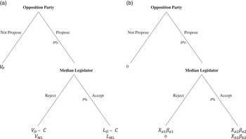
) or accepting the motion (A), leading to outcomes Fail and Pass, respectively. Figure 1(a) shows the formal model. I theorize that the opposition party’s decision to propose or not propose an NCM depends on its value from the current government, V
O
, against the costs of proposing an NCM, C, and the O’s likelihood of being in the post-election government, L
O
. On the other hand, the decision by the median legislator is based on weighing its value from the current government, V
ML
against the likelihood of being in the post-election government, L
ML
.
Theoretical and empirical model of legislative success (a) Theoretical model (b) Empirical model

The simple set of interactions depicted in the formal model has two promising features. First, the model produces clear and concise empirical expectations (see below), which can be easily tested with the appropriate empirical model. Not only can we evaluate the theoretical model based on the underlying logic and intellectual rigor, but also whether its expectations are consistent with the empirical record. Second, the model is simple; it isolates the key actors and their decisions and avoids unnecessary complexity (e.g., party factions, coalition dynamics, repeated interactions, the head of state’s role,Footnote 1 etc). A notable complication is that institutional rules in some states mean that an election may not automatically follow successful NCMs. Although in theory this might influence the opposition’s decision making, of the 12 successes in the sample, only one did not lead to early elections within three months of the NCM’s passage,Footnote 2 which suggests that these institutional effects are likely minimal in practice. Most importantly, the explanatory capacity of this model is directly related to the model’s simplicity, I can effectively predict NCMs generally and their outcomes based on a few theoretical components.Footnote 3 By doing so, we gain additional insight about the process that generates NCMs as well as their outcomes.
Motivating Example
To demonstrate how this simple formal model captures the decision-making process, I briefly describe a series of interactions that profoundly influenced Irish politics. This case illustrates two features that inform our understanding of parliamentary decision making. The first feature is that this case demonstrates a number of components that factor into the decisions of both the opposition party and the median legislator. The second feature is that opposition parties do not make their decisions in a vacuum, but instead anticipate the decisions of key actors—in this case, the median legislator in parliament.
Consider the situation facing the Irish opposition Labour Party in fall 1992. It had observed a massive rift arise between Fianna Fail and its junior partner Progressive Democrats over a public disagreement between the two parties’ leaders. Although the coalition was only nine months old, it had consisted of Fianna Fail “publicly sidelining and denigrating the Progressive Democrats” (Joyce Reference Joyce1992), and had been characterized by Prime Minister Albert Reynolds as being a “temporary little arrangement” (Barrett Reference Barrett1992). At the same time, the Labour Party was in a strong position considering Fianna Fail’s decline in the polls and its potential as a coalition partner for both Fine Gael and Fianna Fail. This, combined with the Progressive Democrats’ anticipated support of the motion, triggered the successful motion on November 5, 1992, a parliamentary dissolution, and the subsequent early election. The move paid off for Labour, as they doubled their seat shares in the Dail (from 15 to 33 out of 166) (Keesing’s World Archives 39208), which placed them in the “kingmaker” role. After negotiations fell through with Fine Gael and Progressive Democrats, Labour eventually formed a coalition with the weakened Fianna Fail ( Keesing’s World Archives 39287).
We can use this case to consider the components that influence the opposition party’s (O) decision to propose an NCM. When deciding whether to propose the motion, the opposition Labour Party considered the two possible eventual outcomes Fail and Pass. If the motion failed, then it would be stuck with the current governing arrangement, for which it had little value (V O ). At the same time, by proposing an NCM, it would have to pay the costs associated with doing so, whether it is through transactions costs (Lupia and Strom Reference Lupia and Strom1995) or more unobservable costs (such as potentially alienating voters) (C). If the motion passed, then Labour would need to consider the likelihood that it was part of the next government (L O ). As a possible coalition partner for both major parties and with large anticipated electoral gains, Labour found itself in an extremely favorable position as a likely part of any post-election government. This decision is made difficult, however, by the uncertainty related to the decision made by the median legislator on this particular issueFootnote 4 —the Progressive Democrats—as they determined whether the motion passed. Consequently, Labour had to weigh the value that it received from having the motion pass by the probability that the Progressive Democrats supported it. Only once the anticipated reaction of the Progressive Democrats is taken into account, does Labour decide that challenging the government makes more sense than abstaining.
The Progressive Democrats held the fate of the government in its hands. Its decision making was rather straightforward. The value that it received from the current governing arrangement was quite small (V ML ), given that the coalition had been slowly deteriorating over the course of its short, nine-month tenure owing to infighting and public disagreements. At the same time, the Progressive Democrats were optimistic about the potential for taking advantage of Fianna Fail’s declining polls and receiving some consideration as a junior coalition partner (L ML ). In the end, the little value that the Progressive Democrats received from the governing arrangement was not enough to prevent it from trying its luck at forming another coalition after the election.
Theoretical Expectations
In this section, I conceptualize the actors’ utilities in the model depicted in Figure 1(a). The selection of the factors that influence these utilities is informed by previous research on parliamentary dissolution and government stability (e.g., Balke 1990; Warwick Reference Warwick1994; Lupia and Strom Reference Lupia and Strom1995; Strom and Swindle Reference Strom and Swindle2002; Kayser Reference Kayser2005). The first component includes the opposition party’s (V O ) and median legislator’s value (V ML ) for the current governing arrangement, which will influence their decisions to propose and to accept the motion, respectively. Both actors compare the value that they receive from the current governing arrangement to what they would expect to get following a successful NCM (e.g., Balke 1990; Lupia and Strom Reference Lupia and Strom1995).
I conceptualize the V parameter as a combination of five government/system characteristics: minority governments, surplus coalitions, number of governing parties, government tenure, and the election cycle. As minority governments have to rely on the support of non-governing parties to remain in office, they are often in a more precarious position in terms of stability (Strom Reference Strom1990). Non-governing parties are more willing to support NCMs because their support is not held in check with the provision of cabinet posts. Moreover, simply having a majority of parliament outside of the governing coalition eases the passage of motions. Thus, opposition parties will be more likely to propose NCMs against minority governments, and median legislators will be more willing to support these motions. On the other hand, some governments may control a parliamentary majority yet still be vulnerable to challenges because one or more parties is unnecessary to maintain the majority. I anticipate that surplus coalitions will face a higher risk of NCMs—relative to more stable types of governments such as single-party majority or minimal winning coalitions (MWCs)—because including unnecessary coalition partners further divides the benefits from holding office (Dodd Reference Dodd1976).
Larger coalitions are also more vulnerable to removal from office, as the governing parties may leave the coalition owing to difficulties in intra-coalition bargaining (Warwick Reference Warwick1994). Although coalition governments may increase the risk of government termination because of replacement, there is a negative relationship between coalition governments and the possibility of early parliamentary dissolution (e.g., Strom and Swindle Reference Strom and Swindle2002; Schleiter and Morgan-Jones Reference Schleiter and Morgan-Jones2009). In addition, having more government parties may reduce the median legislator’s probability of accepting the motion as they may be worried “that internal government problems could manifest themselves negatively at the polls” (Palmer and Whitten Reference Palmer and Whitten2000, 418).
The third element of V captures the time left in the constitutional inter-election period (CIEP). When deciding whether to trigger the dissolution of parliament, the ML must weigh its opportunity costs, or the benefits from the particular coalition that it would pay.Footnote 5 The earlier it is in the election cycle, the greater the government’s opportunity costs of dissolution (e.g., Lupia and Strom Reference Lupia and Strom1995; Diermeier and Stevenson Reference Diermeier and Stevenson2000), and the less likely that the median legislator forgoes those benefits. Opposition parties may realize that the ML will be more willing to accept later on and so they might change their behavior to reflect the likelihood of success. Another motivation flows from Williams (Reference Williams2011), who shows that opposition parties have an incentive to propose NCMs before the election in order to sway voters. If opposition parties are motivated by potential electoral gains or legislative success, then we should see a rise in the number of motions as the electoral clock winds down.
The final element of V is the government’s tenure. Although Warwick (Reference Warwick1994) discovers that the risk of government termination increases as the government ages, this effect may be confounded by the effects of the election cycle (Diermeier and Stevenson Reference Diermeier and Stevenson2000). Once I control for the effects of the election cycle, I expect that younger governments will face a higher risk of NCMs than older governments because they may not have solidified their bases of support. Opportunistic opposition parties might therefore be encouraged to test the strength of the coalition by challenging young governments. This variable also captures the increased instability that is reflected in the shorter durations of younger, mid-cycle replacement governments (Warwick Reference Warwick1994, 35).
The next element of the opposition party’s utility for an NCM includes the costs that it pays to propose. Although proposal costs are largely unobservable, we can include indirect proxies that speak toward the overall propensity for opposition parties to propose NCMs in that system. I theorize that when opposition parties have proposed a large number of NCMs recently, there are lower proposal costs. Moreover, the usage of NCMs in the past should also reflect the costs of challenging the government owing to each country’s institutional variations affecting the ease of tabling a confidence motion. The easier it is to table a motion, the lower the costs associated with doing so.
The utility that O gets from a successful motion is a function of its likelihood of being a part of the post-election government (L O ). Given the close connection between macroeconomic conditions and electoral support (e.g., Powell and Whitten Reference Powell and Whitten1993), it makes sense for the opposition party to consider the state of the economy when determining L O . I expect that stronger economic conditions will reduce the opposition party’s utility of challenging government because the government will likely be in a better electoral position should the motion pass. The second element of L O captures the presence of a large number of coalition alternatives in addition to the opposition party. When there are few alternative parties, opposition parties are more likely to be included in the post-election governing arrangement. Being one of few parliamentary parties means that the opposition party is more likely to benefit from disaffected voters shifting their support away from the government. Much like O, the ML also considers the likelihood or returning to office. In some systems, government terminations are unlikely to permanently displace the government parties owing to a number of systemic factors. In addition to reflecting a lack of alternative coalitions (Warwick Reference Warwick1994, 47), systems where government parties return to office may increase the willingness of the median legislator to support the motion, as it is likely to be a part of the post-election government that follows the parliamentary dissolution.
Data
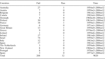
The unit of analysis is the country-month. Table 1 shows the sample of 19 advanced parliamentary democracies, all of which have established party systems where the government is accountable to the parliament.Footnote 6 The sample period under consideration is determined by the availability of GDP data (Germany), the first democratic election (Greece, Japan, Portugal, and Spain), and the availability of NCM data (all end dates). I code three mutually exclusive outcomes (SQ, Fail, and Pass) based on whether an NCM occurs in that month, and whether that NCM was successful. So that the conclusions of this paper are directly comparable, I use Williams (Reference Williams2011) as the source of the data on the timing and outcomes of NCMs, which uses a combination of parliamentary archives and secondary sources (e.g., wire reports, newspaper articles, and Keesing’s World Archives ).Footnote 7
Distribution of No-Confidence Motions Within Sample Countries

Table 1 provides the number of Fail and Pass outcomes for each sample state. Although these are all advanced parliamentary democracies, there exists substantial variation regarding the occurrence and success rates of NCMs. The distribution of NCMs has considerable variance, with some countries challenging often (e.g., Australia and Finland) and others challenging only in unique situations (e.g., Iceland, the Netherlands, and Spain).
In the third column of Table 1, I provide the number of successful NCMs in each country. In order to be coded as a successful NCM, the motion must meet two criteria. The first criterion is that the confidence motion has to originate from an opposition lawmaker or party.Footnote 8 The second criterion that determines a successful NCM is one that causes the termination of government as a direct result of an NCM receiving a majority in a vote. This is distinct from those times in which merely the threat of an NCM is enough to cause the government to preemptively resign. These cases of preemptive resignation are conceptually distinct from those discussed herein because NCMs do not actually get tabled (thus removing the first stage of decision making in Figure 1) and there is virtually no uncertainty regarding the motion’s potential for passage (thus forcing the government’s resignation). In addition, it is often difficult to determine whether the resignation occurred as a preemptive attempt to avoid an NCM or some other coalition dynamic (such as political infighting). As preemptive resignations are most likely produced by a different data-generating process, I only analyze those NCMs where an actual vote occurs. Of these sample countries, NCMs only appear to be successful tools of the opposition in Canada, where 36.4 percent of challenges succeed (4 out of 11). Overall, the success percentage is much lower: 4.3 percent (12 out of 280).
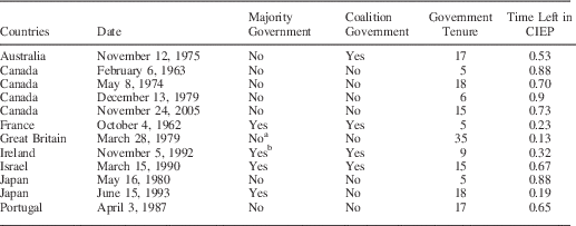
In Table 2, I provide additional information for the 12 successful NCMs in the sample. The most striking feature of this table is that some majority governments are still vulnerable to NCMs. In the case of France, Ireland, and Israel, the government was composed of a coalition of parties that collectively held a majority of seats. Coalition governments are more vulnerable to successful challenges than single-party governments because the benefit to holding office is lower. This, however, does not explain the case of the termination of the single-party majority government of Japan in June 1993. Although the LDP had a majority of seats in the Diet, numerous divisive factions were present in the party. On the day of the vote, 70 members from the two factions, headed by former PMs Takeo Fukuda and Takeo Miki, abstained from the vote, causing the motion to be carried 243 votes to 187. As NCMs in Japan only require a simple majority, abstaining was considered a vote against government ( Keesing’s World Archives 30453). The rest of the columns display the government’s tenure (in months) and the proportion of time left in the CIEP. For the most part, younger governments are more vulnerable to removal, especially later in the election cycle (with a low proportion of time left in the CIEP).
Successful No-Confidence Motions in the Sample
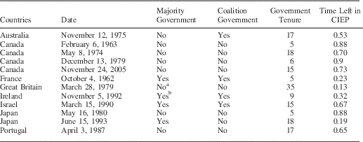
Note: CIEP=constitutional inter-election period.
a Labour originally had a majority following the 1974 election, but was reduced to a minority following defections and by-elections.
b Together, the Fianna Fail–Progressive Democrat coalition controlled 83 of 165 seats, with a Speaker casting a vote in the event of a tie.
Before I explore these patterns in a multivariate analysis, I need to briefly describe the data sources and coding practices for the payoffs of the theoretical model (i.e., V O , C, L O , V ML , and L ML ). I include a number of variables unique to each government to capture the value that actors receive from the current governing arrangement. These variables include an indicator variable representing whether the governing parties do not have majority support in parliament (minority government), whether there are surplus parties in the coalition (surplus government),Footnote 9 the number of parties controlling cabinet portfolios (government parties), and the age of government (in months) (government tenure). I use the studies by Woldendorp, Keman and Budge (Reference Woldendorp, Keman and Budge2000) and Seki and Williams (Reference Seki and Williams2014) as the primary source for government composition values.
The stage of the election cycle can profoundly influence decision making. One way of characterizing the election cycle is illustrated in Strom and Swindle (Reference Strom and Swindle2002, 587), which counts the number of days left in the CIEP. Yet, parliamentary democracies have varying lengths of CIEP, so a government having 36 months left in the CIEP represents a different stage in the election cycle in systems with five-year election cycles compared with those with three-year cycles. I propose a more general measure with the time left in CIEP, which measures the proportion of time left before an election is mandated by the constitution, with values closer to 1, representing earlier in the election cycle (Williams Reference Williams2013).Footnote 10
Various institutional arrangements and norms determine the costliness of challenging the government, and therefore may restrict the opposition’s ability to propose NCMs. I incorporate two variables to measure challenge costs: the time (in months) since the last NCM and the number of previous NCMs for that state. With the use of these variables, we can paint a picture of the propensity for the opposition to challenge governments in that country in the past. I expect that the unit heterogeneity shown in Table 1 will be reflected in states having different values of these two variables, and thus different underlying risks of NCMs (Beck, Katz and Tucker Reference Beck, Katz and Tucker1998).Footnote 11
To measure the likelihood that the opposition party is in the post-election government, I create the effective number of parties, which measures the total party fragmentation of the system. Higher numbers represent more parties and thus a lower utility for the opposition party of a successful NCM (Laakso and Taagepera Reference Laakso and Taagepera1979). To capture the effects of economic performance on electoral support for the government, I include a general measure of the state of the economy, change in real GDP per capita. This is taken from Penn World Table Version 6.2 (Heston, Summers and Aten Reference Heston, Summers and Aten2006). Finally, the ML will be more reluctant to support the motion if it fears being excluded from the post-election government. To measure this possibility, I calculate the returnability index by calculating a rolling percentage of non-caretaker governing parties that are returned to office following an election, up to that point.Footnote 12
Empirical Model
Consider the illustrative case of Labour proposing a successful NCM in Ireland in 1992 as a real-world example of the two-stage interaction depicted in Figure 1(a). I theorize that this formal model produces a simple yet accurate account of the strategic process that generates NCMs in advanced parliamentary democracies. The empirical method used to test these expectations should therefore reflect the actors, choices, sequences, and utilities over outcomes depicted in the formal model.
One possible strategy to empirically test these expectations would be to estimate a logit predicting whether an NCM either passes or fails. Besides distorting the strategic nature of the model by ignoring the opposition party’s initial action (i.e., P or
 $\bar{P}$
), there would be omitted variable bias owing to the nonlinear functional form (Signorino Reference Signorino1999; Signorino and Yilmaz Reference Signorino and Yilmaz2003).Footnote
13
Another option is to estimate a selection model, where the selection stage represents the initial choice by the opposition party (i.e., Labour Party) and the second stage determines its outcome (i.e., Progressive Democrats’ choice). Although this two-stage process is closer to the data-generating process than a logit, it fails to model the expected utility calculations that results in significant bias (Signorino Reference Signorino2002).
For these reasons, I utilize a method that allows me to derive the statistical model directly from the theoretical model (Signorino Reference Signorino1999, 281). Assume that players i={O, ML} have a true utility for action j={SQ, Fail, Pass},
 $$U_{i}^{{\asterisk}} (j)$$
, which is divided into two components: an expected utility component that is observed by all players U
i
(j) and a random component, α
j
, observable only to that player (though the other players know the distribution of α
j
).Footnote
14
By introducing a stochastic component (α
j
) to the utilities, the empirical model generates predictions for all three outcomes, thereby avoiding the pitfalls of unreasonable, deterministic predictions from complete information formal models. A stochastic approach also more closely approximates the informational uncertainty that often plagues inter-party bargaining situations (Strom Reference Strom1994).
I now specify each actor’s utilities over the outcomes in terms of regressors:
 $$U_{O} (Fail)=X_{{a1}} \beta _{{a1}} ,$$
 $$U_{O} (Pass)=X_{{a2}} \beta _{{a2}} ,$$
 $$U_{{ML}} (Pass)=X_{{b2}} \beta _{{b2}} .$$
For identification purposes (see Lewis and Schultz Reference Lewis and Schultz2003), I normalize U O (SQ) and U ML (Fail) to equal 0 and I exclude the constant term from the opposition’s utility.
As O does not observe ML’s choice when making the decision to challenge, O must weigh the utilities that result from P by ML’s action probabilities. If we let pr A be the probability that the ML accepts the motion,Footnote 15 then O’s decision rule is the following:
 $$y_{O} =\left\{ {\matrix{ {P\quad {\rm if}\,(1{\minus}pr_{A} )U_{O} (Fail){\plus}pr_{A} U_{O} (Pass)\gt U_{O} (SQ)} \cr { & \bar{P}\quad {\rm otherwise}} \cr } } \right..$$
The ML’s choice is not strategic (thus the reason why no utilities are given for outcome SQ), but is conditional on the occurrence of an NCM. ML’s decision rule is the following:
 $$y_{{ML}} =\left\{ {\matrix{ {A\quad {\rm if}\,U_{{ML}} (Pass)\gt U_{{ML}} (Fail)} \cr { & \bar{A}\quad} {\rm otherwise} \cr } } \right..$$
After assigning variables to represent utilities (see Figure 1(b)), I solve this recursive system of equations with SBI (Bas, Signorino and Walker Reference Bas, Signorino and Walker2008, 22).Footnote 16 First, start at the bottom node and estimate a logit of ML’s choice given an NCM, and predict pr A . Use pr A to transform O’s utilities over the outcomes that follow P (X a1 and X a2) into expected utilities. Given knowledge of ML’s choice, I then use a logit to estimate the utilities that determine O’s choice to propose at the top node. Thus, the empirical method is similar to the backwards induction technique used to solve game-theoretic models (Bas, Signorino and Walker Reference Bas, Signorino and Walker2008, 22). In the next section, I discuss the empirical results.
Results
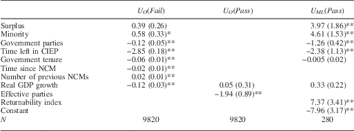
Table 3 provides the results of the SBI for the theoretical model presented in Figure 1. The first column shows the estimates
 $\widehat{{(\beta _{{a1}} }})$
for the opposition party’s utilities for a failed NCM (U
O
(Fail)), and the second column shows the estimates
 $(\widehat{{\beta _{{a2}} }})$
for the opposition party’s utilities for a successful NCM (U
O
(Pass)). The last column provides the estimates
 $(\widehat{{\beta _{{b2}} }})$
for the median legislator’s utility of a successful motion (U
ML
(Pass)). Positive coefficients indicate that the variable increases that actor’s utility for that outcome.
Statistical Backwards Induction Results for the Theoretical Model of No-Confidence Motions Presented in Figure 1
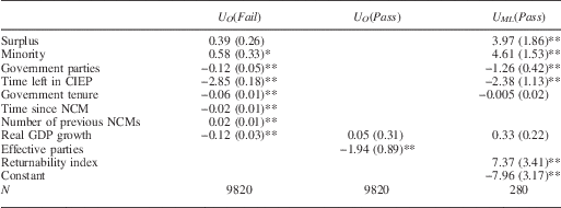
Note: SE in parentheses, the SE for the opposition’s utility are based on 1000 bootstrapped replications. U O (SQ) and U ML (Fail) are constrained to 0 for identification purposes.
CIEP=constitutional inter-election period; NCM=no-confidence motion.
**p<0.05, *p<0.1 (two-tailed).
The Opposition Party’s Utility
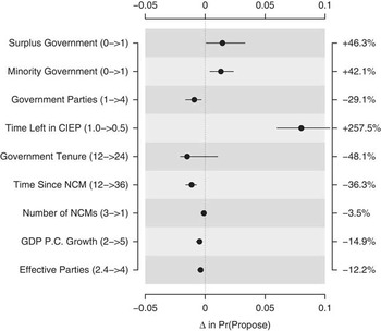
The first stage of the SBI produces estimates for the opposition party’s utility. I theorize that the opposition will be more likely to challenge government as its value from the current government (V O ) decreases, proposal costs (C) decrease, and the likelihood of being in the post-election government (L O ) increases. Based on the first two columns, I conclude that opposition parties receive greater utility, and are thus more likely to propose an NCM, when facing (a) minority government,Footnote 17 (b) late in the election cycle, (c) young government, (d) in a state with a recent NCM, (e) in a state with a high number of previous NCMs, (f) with low economic growth, and (g) few parliamentary parties.
Much like coefficients in a traditional logit or probit, the interpretation of the substantive effects is more intuitive by examining the predicted action probabilities.Footnote 18 Figure 2 shows the changes in predicted probabilities of an opposition party proposing an NCM (and 95 percent confidence intervals) as we vary the values of the statistically significant explanatory variables in meaningful ways. It is important to note that the changes in predicted probabilities reflect holding pr A constant at an “average” expectation of the motion’s success (the sample mean of pr A is 0.043 and the standard deviation is 0.10, which is consistent with the relative rarity of successful NCMs).Footnote 19 The baseline probability of an opposition party proposing an NCM in a given month (pr P ) is 0.031.Footnote 20
Changes in the probability of opposition proposing a no-confidence motion (pr P ) over the baseline probability (pr P =0.03) Note: lines represent 95 percent confidence intervals. Percentages represent change over the baseline probability.

I theorize that variables increase the opposition party’s utility for a failed NCM in two ways: by decreasing the value that the opposition party gets from the current governing arrangement (V O ) and by reducing proposal costs (C). For the most part, we see evidence consistent with these expectations. Surplus governments increase the utility of proposing an NCM relative to the reference category (single-party majorities and MWCs) by 46.3 percent over the baseline scenario. Moreover, facing a government without majority support increases the probability of proposing by 0.013, which is a substantively large decrease of 42.1 percent compared with the baseline scenario. As shown in Table 3, high rates of economic growth reduce the probability of an NCM by decreasing the opposition’s utility of a failed NCM (first column) rather than the opposition’s utility of a successful NCM (second column).
Opposition parties become less willing to challenge as governments age because it becomes obvious that other coalition arrangements are not preferred to the current one by the government parties. Governments that are two years old have a 0.015 lower probability of being challenged than one-year-old governments (a decrease of 48.1 percent). The final variable in X a1 that measures value is the time left in CIEP. Moving halfway through the election cycle increases the probability by 0.08 (a 257.5 percent increase). When viewed in tandem, it appears as though time—as both tenure and the stage of the electoral cycle—has counter-balancing effects on the opposition’s incentive to propose NCMs. In the Discussion section, I further explore how these results influence opposition behavior throughout the electoral cycle.
Increased proposal costs decrease the opposition party’s utility for a failed NCM. Increasing the time since the previous NCM from 12 to 36 months decreases the probability by 0.011 (a 36.3 percent decrease), whereas having fewer NCMs in the past (one compared with three) decreases the probability by 0.001 (a 3.5 percent decrease). Finally, the effective number of parliamentary parties influences the probability of an NCM by changing the opposition party’s likelihood of being in the next government following an election (X a2). Increasing the effective number of parliamentary parties from 2.4 to 4 makes the opposition less willing to pay the costs of challenging, as there are more governing options that do not include them. It also provides support for the electoral motivation for challenging as opposition parties are more likely to see an electoral boost in systems with a small number of parliamentary parties (Williams Reference Williams2011).
The Median Legislator’s Utility
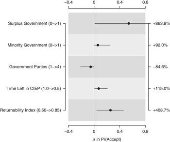
Once the opposition party proposes an NCM, the median legislator is faced with the choice of accepting the motion (at which point it passes) or rejecting the motion. More formally, the median legislator will accept the motion when X b2 β b2>0. X b2 is a function of two components: the median legislator’s value of the current governing arrangement (V ML ) and its likelihood of being in the next government (L ML ). The baseline probability of pr A is 0.063.Footnote 21 I present the substantive effects of these variables in Figure 3.
Changes in the probability of median legislator accepting a no-confidence motion (pr A ) over the baseline probability (pr A =0.063) Note: lines represent 95 percent confidence intervals. Percentages represent change over the baseline probability.

The surplus, minority, and time left in CIEP variables demonstrate that when the median legislator gets greater value from the government it becomes less likely to accept the motion. The relative dearth of successful NCMs against single-party majority governments (i.e., 1 out of 12) and MWC (i.e., 0 out of 12) means that facing a surplus coalition (rather than either a single-party majority or MWC) drastically increases the probability of a successful NCM by a probability of 0.54 (or a substantive increase of 863.8 percent over the baseline scenario). Minority governments increase the probability by 0.058, a substantively large decrease (92.0 percent). As half the election cycle elapses (i.e., when time left in CIEP goes from 1 to 0.5), the median legislator’s utility of accepting the motion increases by 0.072 (an increase of 115.0 percent), which coincides with the opposition’s incentive to propose. At the same time, although the median legislator is likely to get less value of a coalition government (i.e., when number of government parties exceeds 1), they become less likely to accept the motion. The final component of X b2 captures the median legislator’s likelihood of being in the post-election government that follows a successful NCM. As the returnability index increases from 0.5 to 0.85, the probability of accept increases by 0.256 (a 408.7 percent increase). The tremendous influence of this variable is understandable, as the median legislator is more willing to forgo the current benefits if it is confident that it will be in the next government (Warwick Reference Warwick1994).
Discussion
In this section, I reexamine the central motivation for this research: what determines the occurrence and success of NCMs? As I theorize that the outcome of NCMs is a function of choices made by both the opposition party and the median legislator, we can address this puzzle by considering two secondary questions. First, what motivates opposition parties to propose NCMs? Second, what incentives do median legislators have in supporting these motions? As I will show, since strategic considerations guide these actions, the SBI technique is uniquely situated to answer these questions. To address this first question, recall that I theorized that opposition parties would be more likely to propose early in the government’s tenure and early in the election cycle, because these are the times when it receives less value from the current governing arrangement.Footnote 22 To examine whether the empirical results are consistent with these expectations, I produce two figures.
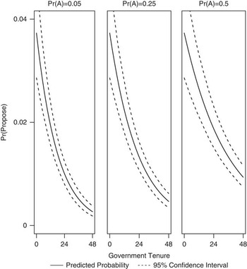
Figure 4 provides the probability of an opposition party proposing an NCM (and 95 percent confidence intervals) across a 48-month government. As these are represented with expected utilities, I produce three figures based on different expectations of the probability of the median legislator accepting the motion (pr A ). The first panel shows a situation where the opposition anticipates failure, the second panel is more favorable, and the final panel shows an extremely favorable situation (a basic coin flip).Footnote 23
Probability of opposition proposing a no-confidence motion (pr P ) across government tenure for three different values of probability of accept (pr A )

We can draw two main inferences from Figure 4. First, in all three panels, the probability of proposing is highest early in the government’s tenure and then decreases as the government ages. Although this echoes Diermeier and Stevenson’s (Reference Diermeier and Stevenson2000) finding that the highest rate for dissolution is within the first year of the government’s tenure, it contradicts Warwick’s (Reference Warwick1994) observance of rising hazards. Second, and perhaps more interestingly, the expected probability of the motion’s success (pr A ) can potentially change this calculation. By looking across panels, we can see that when governments are young, the probability of proposing is similar, regardless of the motion’s potential for success. The chance of success (i.e., pr(A)) has its largest impact when governments are older, at which point opposition parties become more willing to propose when passage is most likely. In the case of government tenure, it looks like opposition parties are timing their NCMs to coincide with the highest chance of success.
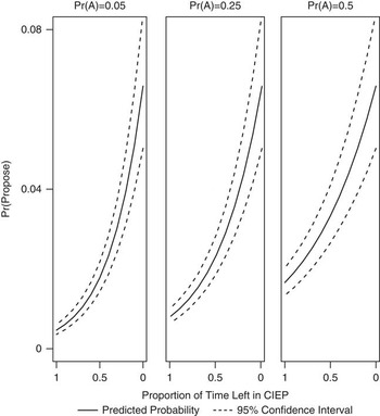
On the other hand, in Figure 5, we see puzzling behavior. Opposition parties are most likely to challenge late in the election cycle (with values of time left in CIEP closer to 0). This by itself is not puzzling, given the theoretical expectations (e.g., Balke 1990; Lupia and Strom Reference Lupia and Strom1995; Baron Reference Baron1998) and previous empirical results (e.g., Diermeier and Stevenson Reference Diermeier and Stevenson2000; Palmer and Whitten Reference Palmer and Whitten2000; Strom and Swindle Reference Strom and Swindle2002). The puzzle arises when we consider that this is the stage of the election cycle when the government is likely to be replaced anyway. There are two possible explanations for this result. The first explanation is that this is the period when the ML is most likely to accept the motion, in this case, opposition parties are behaving strategically based on legislative success. The other possible explanation for this puzzling behavior is that opposition parties are responding to the potential electoral benefits of challenging the government immediately before an election (Williams Reference Williams2011). The NCMs act as signals of the opposition party’s abilities to govern vis-à-vis the current government, which voters use when deciding which party to support. Indeed, by examining the slopes we can infer that the election cycle has the largest impact on the probability of proposing when the motion is likely to fail, and the smallest impact when success is likely. In other words, opposition parties challenge late in the election cycle in the face of almost certain failure because there is the possibility of influencing voters at the next election (i.e., “electoral success”).
Probability of opposition proposing a no-confidence motion (pr P ) across the electoral cycle for three different values of probability of accept (pr A )

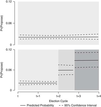
When we examine both of these motivations in tandem, we gain insight as to why successful NCMs are so rare. Consider how the probability of propose (and 95 percent confidence intervals) changes for a hypothetical government formed immediately after an election. Each month the government is in office its tenure (i.e., government tenure) increases, which decreases its risk of a challenge. At the same time, each subsequent month in office brings the government closer to having to call an election (i.e., time left in CIEP decreases), which increases its risk of a challenge.Footnote 24 The top panel of Figure 6 shows that the probability of propose in this basic scenario does not change significantly over the government’s time in office. When opposition parties have the greatest motivation for legislative success and want to challenge a young government, there is little incentive because voters are unlikely to reward an NCM so far from the election. As the next election approaches, when the electoral success motivation is greatest, opposition parties do not see the value in challenging a well-established government.
The probability of opposition proposing a no-confidence motion (NCM, pr P ) for one government (top panel) versus three governments illustrates the contrasting effects of government tenure and election cycle Note: this figure depicts the predicted probability (and 95 percent confidence interval) of an opposition party proposing an NCM across four time periods in an election cycle (t, …, t+4) for two scenarios. The top panel represents one government; the bottom panel depicts three otherwise identical governments (represented by shaded regions) replaced throughout the election cycle. Only the values of government tenure and time left in CIEP vary. CIEP=constitutional inter-election period.

The bottom panel of Figure 6 shows how this dynamic changes when there are multiple governments (represented by the shaded areas) owing to coalition reorganization (replacement) over the course of an election cycle. The first government faces nearly the same threat of an NCM throughout its tenure (first half of the election cycle). This result is consistent with the rationale that “postelection governments benefit from a ‘honeymoon effect’: legislators may be more reluctant to bring postelection governments down because they reflect, in some fashion, the electorate’s will” (Warwick Reference Warwick1994, 35; see also Diermeier and Stevenson Reference Diermeier and Stevenson1999). When the second government comes into office, with all else equal, opposition parties are emboldened by facing a younger and potentially more vulnerable government. The last government is most susceptible to NCMs because it rewards both types of motivation: legislative success (by facing a younger government) and electoral success (by proposing close to an election). The dual incentives of legislative and electoral success, in combination with the median legislator’s incentives, provide insight for the rarity of successful NCMs.
The second question to explore is to consider when the median legislator is most likely to accept the NCM. Although it only takes one opposition party to decide to challenge the government, it takes a median legislator to agree to cast the vote that gives the no-confidence vote a majority. Therefore, a successful NCM requires compatible actions by two actors. In some situations, having two diverse actors agree on an NCM is simpler because they are both in the opposition. Opposition parties’ behaviors are consistent with the anticipated probability of success in terms of challenging governments without majority support and governments late in the election cycle. By examining the effects of government characteristics it becomes clear that opposition parties and median legislators respond to government characteristics differently based on their incentives. More specifically, we see that whereas the age of government encourages NCMs, it has no impact on their success. Likewise, whereas coalition governments do not encourage NCMs, they do reduce their success rate.
Therein lies a puzzling phenomenon: what explains the fact that successful NCMs are extremely rare in advanced parliamentary democracies? In order for NCMs to be successful, there must be the incentive for an opposition party and a median legislator—most often in different parties—to support bringing down the government. Needless to say, this is a difficult task for two primary reasons. First, as illustrated above, opposition parties are not solely motivated by bringing down the government. This means that they do not only challenge the government when it has its highest level of success, but also when it justifies electoral goals. Second, an opposition party and the median legislator may react to governing arrangements differently, making coordination between the two increasingly difficult. This study explains this puzzle in that the times in which opposition parties have the most incentive to challenge the government are also those where the median legislator does not want to rock the boat by bringing down the government.
Implications and Conclusion
This project identifies the conditions under which opposition parties propose NCMs and the determinants of their success. I develop a simple theoretical model of legislative success based on the incentives of the opposition and the median legislator. I then test those theoretical expectations with an empirical model that is explicitly derived from the underlying theoretical model. As such, it represents the first empirical examination of how the behaviors of opposition parties change as a result of policy performance and institutional structures. I find that NCMs are more likely against young, minority governments, when the proposal costs are low, in states with few parliamentary parties, and late in the election cycle. NCMs are more likely to be successful against minority or surplus governments, late in the election cycle, and when there is a high probability that the median legislator is in the next government.
We can understand the opposition’s behavior as a combination of both the potential to trigger the government’s downfall (legislative success) and the incentive to improve its electoral position (electoral success). For example, I find that the influence of the electoral cycle is inversely related to the motion’s likelihood of success. In other words, the stage of the electoral cycle has the biggest influence when the motion is unlikely to pass, a pattern that is consistent with opposition parties being motivated by the prospects of electoral success. Inconsistent findings on the relationship between time and government stability (e.g., Warwick Reference Warwick1994; Diermeier and Stevenson Reference Diermeier and Stevenson2000) can thus be partially explained by the contrasting influences that government tenure and electoral cycle have on the decision to propose NCMs. As the outcome of NCMs is the result of both actors’ behaviors, the rarity of successful NCMs can be explained by the difficult process of aligning the actors’ incentives so that they are compatible.
By examining successful NCMs, we can gain intuition about a type of government termination that, whereas formalized in some models (e.g., Strom Reference Strom1994; Baron Reference Baron1998), is often lumped together with other types in empirical examinations of government failure (e.g., Warwick Reference Warwick1994). These are substantively meaningful types of terminations that are the result of different sets of interactions between key actors, and thus should be evaluated separately. Incorrectly aggregating these types of terminations can potentially risk misleading inferences. For example, whereas the state of the economy is typically identified as a catalyst for strategic election timing (e.g., Smith Reference Smith2003), the results here suggest that the economy has little impact on terminations related to lack of parliamentary confidence (though a poor economy increases the probability of proposing). Thus, a particularly fruitful endeavor would be to examine the catalysts for different types of termination beyond simply replacement or dissolution (Diermeier and Stevenson Reference Diermeier and Stevenson1999). At the very least, this project represents a call to devote more theoretical and empirical attention to explaining opposition behavior, especially given the opposition’s role in triggering early elections through parliamentary dissolution (e.g., Strom and Swindle Reference Strom and Swindle2002; Schleiter and Morgan-Jones Reference Schleiter and Morgan-Jones2009).