



1. Introduction
Micro-air vehicles (MAVs) represent a significant frontier in advanced aircraft technology. Due to their small size and low flight speeds, these vehicles usually operate at low Reynolds numbers. At this range, complex flow phenomena such as laminar separation, transition and reattachment can lead to deteriorated aerodynamic performance (Mueller & DeLaurier Reference Mueller and DeLaurier2003; Pines & Bohorquez Reference Pines and Bohorquez2006). Bio-inspired flexible membrane wings present a promising solution to these challenges (Shyy, Ifju & Viieru Reference Shyy, Ifju and Viieru2005). By allowing for passive, flow-induced deformation, these wings can help suppress flow separation, enhance lift and delay stall, while their lightweight construction and low cost further strengthen their appeal for MAV applications.
Most existing studies on the flow–structure interaction of membrane wings have focused on simplified configurations, typically two-dimensional single-layer membranes with fixed leading and trailing edges, or rectangular membranes constrained along their perimeter. Unlike rigid flat-plate wings, membrane wings can develop significant camber in response to the pressure differential between their upper and lower surfaces, thereby increasing lift and delaying stall. Assuming a uniform pressure distribution and a circular arc membrane shape, both the membrane curvature and the resulting lift can be predicted using a single non-dimensional parameter, such as the Weber number
 $We$
, which compares aerodynamic loading with membrane elasticity, or the aeroelastic parameter
 $Ae$
, which relates membrane compliance to the dynamic pressure (Song et al. Reference Song, Tian, Israeli, Galvao, Bishop, Swartz and Breuer2008; Waldman & Breuer Reference Waldman and Breuer2017).
Beyond static deformation, increasing attention has been devoted in recent years to the role of unsteady membrane vibration and its influence on aerodynamic performance and flow–structure interaction. Both experimental and numerical investigations demonstrated that membrane vibration, even when the time-averaged camber is matched to that of a rigid wing, can suppress flow separation and delay stall by promoting the formation of large vortices over the wing at high angles of attack (Gordnier Reference Gordnier2009; Rojratsirikul, Wang & Gursul Reference Rojratsirikul, Wang and Gursul2009). Subsequent investigations examined the influence of key structural parameters, such as membrane pre-strain and aspect ratio, on vibration behaviour and aerodynamic response (Rojratsirikul et al. Reference Rojratsirikul, Wang and Gursul2010, Reference Rojratsirikul, Genc, Wang and Gursul2011; Gordnier & Attar Reference Gordnier and Attar2014). Further studies revealed that the coupled flow–structure system often exhibits frequency lock-in among aerodynamic forces, membrane vibration and vortex shedding. The associated dominant frequencies are closely related to the spatial vibration modes and natural frequencies of the membrane, and are influenced by parameters such as angle of attack, Reynolds number and aeroelastic coefficient (Bleischwitz, de Kat & Ganapathisubramani Reference Bleischwitz, de Kat and Ganapathisubramani2015; He & Wang Reference He and Wang2020, Reference He and Wang2023; Li, Jaiman & Khoo Reference Li, Jaiman and Khoo2021). This behaviour has been attributed to a feedback loop involving membrane-vibration modes, vortex shedding and surface-pressure fluctuations (Li, Jaiman & Khoo Reference Li, Jaiman and Khoo2022). However, some studies have also reported that intermittent interactions between leading-edge and trailing-edge flow structures can lead to a mismatch between the dominant frequencies of the flow field and the membrane vibration (Rodríguez-López et al. Reference Rodríguez-López, Carter and Ganapathisubramani2021; He & Wang Reference He and Wang2020, Reference He and Wang2023). While membrane vibration can enhance aerodynamic performance at high angles of attack, numerical simulations have shown that, at low angles of attack, flow–structure interaction induces upstream-propagating pressure waves that may reduce aerodynamic efficiency (Serrano-Galiano, Sandham & Sandberg Reference Serrano-Galiano, Sandham and Sandberg2018). In addition, several studies have also explored the potential of harnessing flow-induced membrane vibrations for energy harvesting, analysing both the dominant vibration frequencies and the corresponding energy-conversion efficiency (Huang et al. Reference Huang, Xia, Dai, Yang and Wu2021b ; Xia et al. Reference Xia, Huang, Dai, Yang and Wu2023). Despite this extensive body of literature, such single-layer membrane wings are typically very thin and therefore susceptible to leading-edge separation (Gordnier Reference Gordnier2009; Rojratsirikul et al. Reference Rojratsirikul, Wang and Gursul2009; Serrano-Galiano & Sandberg Reference Serrano-Galiano and Sandberg2016). The slender supporting frames may also vibrate (Arbós-Torrent et al. Reference Arbós-Torrent, Ganapathisubramani and Palacios2013) or even sustain structural damage due to membrane motion and unsteady aerodynamic loading, limiting their practical applicability.
To better represent realistic aerodynamic configurations, a limited number of studies have incorporated partially flexible membranes into otherwise rigid airfoils. Early numerical simulations by Shyy et al. (Reference Shyy, Klevebring, Nilsson, Sloan, Carroll and Fuentes1999) and Levin & Shyy (Reference Levin and Shyy2001) on a CLARK-Y airfoil with a massless, flexible membrane on the upper surface showed that the membrane effectively increased the average power index of the airfoil and mitigated abrupt lift fluctuations in oscillating free stream. In recent years, Açıkel & Genç (Reference Açıkel and Genç2018) conducted experiments on a NACA4412 airfoil partially covered with a latex rubber membrane. They discovered that, at low Reynolds numbers, this membrane could suppress laminar separation near the trailing edge, thereby improving the lift-to-drag ratio. However, as the Reynolds number increased, the membrane negatively affected aerodynamic performance. Sun et al. (Reference Sun, Zhang, Su and Huang2022) conducted experimental studies and demonstrated that a highly flexible polydimethylsiloxane (PDMS) membrane applied near the leading edge of a NACA0012 airfoil suppressed separation and delayed stall. While these studies underscored the potential aerodynamic benefits of partial membrane constructions, their analyses focused mainly on force measurements and flow visualisation, offering limited insight into the underlying flow–structure interaction mechanisms.
He et al. (Reference He, Guo, Xu, Feng and Wang2023) further applied a thermoplastic polyurethane (TPU) membrane on the leeward surface of a NACA0012 airfoil and implemented active deformation control. They demonstrated that high-frequency actuation effectively suppressed flow separation, thereby enhancing aerodynamic performance. Their results also indicated a strong coupling among the membrane motion, aerodynamic forces and flow structures. However, the Young’s modulus of the membrane used in their study (
 $E = 31.2$
MPa) was significantly higher than that of the membranes employed by Açıkel & Genç (Reference Açıkel and Genç2018) and Sun et al. (Reference Sun, Zhang, Su and Huang2022) (
 $E = 2.2$
and
 $E = 1.2$
–
 $2.3$
MPa, respectively), such that passive deformation exerted a negligible influence on the aerodynamic response. As a result, the influence of highly flexible membranes on airfoil aerodynamics and the underlying flow–structure interaction is still not fully understood and warrants further investigation.
To gain a more comprehensive understanding of the flow-control mechanism of flexible membranes, the present study employs a highly flexible PDMS membrane, whose Young’s modulus is comparable to that of Açıkel & Genç (Reference Açıkel and Genç2018) and Sun et al. (Reference Sun, Zhang, Su and Huang2022), mounted on a NACA0012-based airfoil following the configuration of He et al. (Reference He, Guo, Xu, Feng and Wang2023). Wind-tunnel experiments are conducted with time-resolved, simultaneous measurements of aerodynamic forces, membrane deformation and the surrounding flow field. Based on these measurements, the influence of the local flexible membrane leeward surface on airfoil aerodynamic performance and the underlying mechanisms are systematically investigated.
The paper is organised as follows. Section 2 introduces the experimental set-up, including the models and measurements. Section 3 presents the main statistical characteristics of the experimental results and examines the effects of the flexible membrane through comparisons with a rigid airfoil. Section 4 provides an in-depth analysis and discussion of the flow–structure interaction characteristics and the associated flow-control mechanisms. Finally, § 5 summarises the main conclusions.
2. Experimental set-up
The experiments were conducted in the low-speed, open-loop, and closed-jet wind tunnel at Beihang University. The test section has a rectangular cross-section of 0.43 m
 $\times$
0.50 m and a total length of 5 m. The free-stream velocity
 $U_\infty$
is adjustable within the range of 0–50 m s−1, and the turbulence intensity remains below 0.4 % when
 $U_\infty \gt 7$
m s−1.
Schematic diagram of the experimental set-up: (a) cross-section of the flexible membrane airfoil; (b) schematic of the experimental model and equipment installation; (c) particle image velocimetry measurement plane.

Figure 1. Long description
Panel A: A cross-section diagram of a flexible membrane airfoil. The airfoil is labeled as NACA0012 and features a PDMS membrane. The diagram includes axes labeled x, y, x_trans, and y_trans, with an angle of attack denoted by alpha. Panel B: A schematic of the experimental model and equipment installation. The setup includes an electric turntable, insulated connector, load cell, clamp, model, laser, endplate, and camera. The flow direction is indicated by U_infinity. Panel C: A diagram of the particle image velocimetry measurement plane. The model is positioned within a field of view illuminated by a laser sheet, with dimensions of 225 mm by 225 mm and a model length of 120 mm. The flow direction is indicated by U_infinity.
2.1. Model configuration and installation
This experiment employed two models for comparative investigation: a rigid airfoil, and a flexible membrane airfoil featuring a local flexible membrane on its leeward surface. Both models have a chord length of
 $c = 120$
mm and an effective span of
 $s = 440$
mm, resulting in an aspect ratio of approximately 3.7. This aspect ratio is slightly larger than the value of approximately 3 adopted in the quasi-two-dimensional membrane-wing experiments of Rojratsirikul et al. (Reference Rojratsirikul, Wang and Gursul2009, Reference Rojratsirikul, Wang and Gursul2010), Arbós-Torrent et al. (Reference Arbós-Torrent, Ganapathisubramani and Palacios2013), He & Wang (Reference He and Wang2020, Reference He and Wang2023). The experiments were conducted at a free-stream velocity of
 $U_\infty = 7.5$
m s−1, corresponding to a Reynolds number of
 $Re = 6.0 \times 10^4$
based on the chord length.
The rigid airfoil featured a complete NACA0012 profile, while the cross-section of the flexible membrane airfoil is illustrated in figure 1(a). A cavity was machined on the leeward side of the rigid airfoil, ranging from 16.7 % to 83.3 % of the chord length, with the depth extending down to the airfoil centreline, yielding an effective membrane length of
 $L_m = 80.1$
mm. Small steps approximately 5 mm wide and 0.2 mm deep were added before and behind the cavity, allowing the membrane to be bonded securely. In addition, along the spanwise boundaries of the membrane, a transparent adhesive tape 8 mm in width was applied across the membrane and attached to the leading and trailing edges of the airfoil to suppress possible large deformations and vibrations near the membrane edges. The membrane material was PDMS with a thickness of
 $t_m = 0.2$
mm, density of
 $\rho _m = 1.01$
g cm
 $^{-3}$
and Young’s modulus of
 $E = 1.7$
MPa. This modulus is approximately one-twentieth of that used in the TPU membrane described by He et al. (Reference He, Guo, Xu, Feng and Wang2023), which has
 $E = 31.2$
MPa. The corresponding aeroelastic parameter (Smith & Shyy Reference Smith and Shyy1996), which characterises the relative magnitude of membrane stiffness with respect to the free-stream dynamic pressure
 $q$
, is
 $\varPi _1 = (Et_m/qc)^{1/3} = 4.4$
.
To clearly describe the flow field and membrane deformation in the following text, two plane coordinate systems are defined on the airfoil cross-section, as illustrated in figure 1(a). The first is the
 $x$
–
 $y$
coordinate system, with its origin at the leading edge of the airfoil. The
 $x$
-axis is aligned with the free-stream direction, while the
 $y$
-axis is perpendicular to it, pointing toward the leeward side of the airfoil. The second is the
 $x_{\textit{trans}}$
–
 $y_{\textit{trans}}$
coordinate system, whose origin is placed at the leading edge of the flexible membrane. The
 $x_{\textit{trans}}$
-axis extends along the line connecting the leading and trailing edges of the membrane, while the
 $y_{\textit{trans}}$
-axis is perpendicular to the
 $x_{\textit{trans}}$
-axis and points outward from the leeward surface. The membrane displacement in the
 $y_{\textit{trans}}$
direction is denoted by
 $\eta _{\textit{trans}}$
.
The test model was installed vertically through the upper wall of the wind tunnel into the test section, as shown in figure 1(b). The model was supported from above by a clamp connected to a load cell, and for the flexible membrane airfoil, the internal cavity was vented to the atmosphere near the clamp. The angle of attack was controlled using an electric turntable, adjustable from
 $\alpha = 0^\circ$
to
 $25^\circ$
with a minimum increment of
 $1^\circ$
and an accuracy of
 $\pm 0.01^\circ$
. The reference position of
 $\alpha = 0^\circ$
was determined as the condition at which the measured lift of the rigid airfoil was approximately zero. An insulated connector was placed between the load cell and the electric turntable to eliminate electromagnetic interference. An endplate was mounted at the bottom of the model to suppress three-dimensional flow around the wing tip and to reduce the impact of the boundary layer of the wind-tunnel wall.
2.2. Measurement systems
The aerodynamic forces of the experimental airfoils at various angles of attack were first measured. An ATI Mini40 six-component load cell was employed, providing a measurement range of 20 N and a resolution of
 $5 \times 10^{-3}$
N. Data acquisition was accomplished using an NI USB-6259 acquisition card in conjunction with LabVIEW software. The sampling frequency was set to 4 kHz. Each measurement session lasted 45 s and was repeated three times to ensure data reliability.
Based on variations in aerodynamic forces, particle image velocimetry (PIV) measurements were conducted at the mid-span cross-section in specific cases. These measurements enabled simultaneous acquisition of membrane deformation and velocity fields. A Beamtech Vlite-Hi-527-30 high-speed double-pulse laser was employed to illuminate the desired plane, with a laser sheet thickness of approximately 1.5 mm. Propylene glycol droplets produced by an AG 3000 W heating smoke generator were used as tracer particles, with an average diameter of approximately
 $1 \times 10^{-6}$
m. The PIV image pairs were recorded using a Photron FASTCAM Nova R2 high-speed CMOS camera positioned under the wind tunnel. The optical axis of the camera was aligned perpendicular to the imaging plane, allowing simultaneous capture of the instantaneous tracer-particle distribution and the instantaneous position of the membrane. Each measurement session obtained 5447 image pairs and was repeated twice. The PIV sampling frequency was set to 625 Hz, substantially higher than the dominant frequency of membrane vibration (below 50 Hz near stall; see § 4.1), thereby satisfying the requirements for time-resolved measurements. The PIV field of view, shown in figure 1(c), covered an area of
 $225 \times 225$
mm
 $^2$
. The camera resolution was
 $2048 \times 2048$
pixels, corresponding to a physical magnification of 0.110 mm/pixel.
The original velocity fields were obtained from the recorded raw particle images using the multi-pass iterative Lucas–Kanade algorithm, accelerated by graphics processing units (Champagnat et al. Reference Champagnat, Plyer, Le Besnerais, Leclaire, Davoust and Le Sant2011; Pan et al. Reference Pan, Xue, Xu, Wang and Wei2015). The interrogation window size was set to
 $32 \times 32$
pixels with an overlap of 75 %. By employing sub-pixel interpolation and multi-grid iterations with window deformation, the uncertainty in particle displacement was less than 0.1 pixels. Following the uncertainty-estimation procedure of Qu et al. (Reference Qu, Wang, Feng and He2019), this yields an estimated uncertainty in the PIV velocity measurements of approximately 1.0 % relative to the free-stream velocity
 $U_\infty$
.
Furthermore, the membrane deformation was obtained using a boundary recognition algorithm, as detailed in previous works (Hu, Feng & Wang Reference Hu, Feng and Wang2020; He & Wang Reference He and Wang2020; He, Guo & Wang Reference He, Guo and Wang2022). The main procedure is as follows. First, the raw images are converted into binary images by setting a grey-scale threshold, and the generated connected components are filtered to eliminate tracer particles, retaining only the valid image region near the membrane. Subsequently, the membrane position is identified by locating local maxima in the grey-scale values. Finally, the instantaneous membrane curve is obtained by interpolation and polynomial fitting methods. This algorithm achieves pixel-level accuracy, and based on the camera magnification in this study, the associated uncertainty is approximately 0.09 % relative to the chord length
 $c$
.
3. Aerodynamic effects of membrane flexibility
This section quantifies the aerodynamic impact of the flexible membrane over the full experimental range of angles of attack. The observed aerodynamic trends are then related to the accompanying statistical characteristics of membrane deformation and the surrounding flow field.
3.1. Aerodynamic forces
We first examine the aerodynamic characteristics to establish a baseline for assessing the effects of the flexible membrane. The aerodynamic coefficient curves of the rigid and flexible membrane airfoils are presented in figure 2. As shown in figure 2(a), the lift coefficient of the rigid airfoil follows the trend reported by Ohtake, Nakae & Motohashi (Reference Ohtake, Nakae and Motohashi2007) at a comparable Reynolds number, providing validation of the present measurements. In contrast, the introduction of the flexible membrane significantly modifies the lift response, with effects that depend strongly on the angle of attack. The observed behaviour can be broadly classified into four distinct regimes.
Airfoil aerodynamic characteristics: (a) lift coefficient; (b) drag coefficient; (c) lift-to-drag ratio; (d) lift coefficient increment.

Stage I (
 $\alpha \lt 2^\circ$
): at very low angles of attack, the rigid airfoil produces nearly zero lift. In contrast, the flexible membrane airfoil exhibits a pronounced lift increase: at
 $\alpha = 0^\circ$
, its lift coefficient matches that of the rigid airfoil at approximately
 $\alpha \approx 1.2^\circ$
. This result suggests that an aircraft equipped with flexible membrane wings could operate at a lower installation angle, potentially improving cruise efficiency.
Stage II (
 $2^\circ \leqslant \alpha \lt 10^\circ$
): in this pre-stall regime, the flexible membrane airfoil produces slightly lower lift than the rigid airfoil, while exhibiting a slightly higher drag coefficient (figure 2
b). At
 $\alpha = 10^\circ$
, which corresponds to the stall angle
 $\alpha _{{s},{r}}$
of the rigid airfoil, the lift difference between the two airfoils becomes small. Nevertheless, the flexible membrane airfoil achieves a substantially lower drag coefficient.
Stage III (
 $10^\circ \lt \alpha \leqslant 13^\circ$
): notably, the flexible membrane sustains lift growth beyond the stall of the rigid airfoil, producing a distinct stall-delay regime. Whereas the rigid airfoil stalls at
 $\alpha = 10^\circ$
, the flexible membrane airfoil continues to increase lift up to
 $\alpha = 13^\circ$
, yielding a
 $3^\circ$
stall delay and a 12.4 % increase in the maximum lift coefficient. This behaviour demonstrates a marked improvement in stall performance, highlighting the primary aerodynamic benefit of the flexible membrane.
Stage IV (
 $\alpha \gt 13^\circ$
): in the post-stall regime, once the flexible membrane airfoil also stalls, its lift coefficient converges toward that of the rigid reference, while maintaining a marginally lower drag coefficient.
It is interesting to note that the flexible membrane yields the most pronounced aerodynamic benefits in stages I and III, as evidenced by the enhanced lift-to-drag ratio in figure 2(c).
In comparison, the TPU material membrane used in He et al. (Reference He, Guo, Xu, Feng and Wang2023) shows a similar trend. There is a slight reduction in lift pre-stall, followed by a minor recovery after stall, as shown in figure 2(d). However, the overall impact is much less significant, lacking a measurable stall-delay effect. These findings suggest that a more flexible membrane could be more effective at enhancing stall characteristics, although it might also increase the loss of aerodynamic efficiency pre-stall.
Based on the aerodynamic characteristics outlined above, five representative angles of attack are mainly selected for a detailed examination of membrane deformation and the flow field:
 $\alpha = 0^\circ$
,
 $6^\circ$
,
 $10^\circ$
,
 $13^\circ$
and
 $19^\circ$
. These cases respectively correspond to stage I (very low angle of attack), stage II (pre-stall), the stall angle of the rigid airfoil, stage III (stall-delay) and stage IV (post-stall).
3.2. Membrane deformation
The deformation characteristics of the membrane change significantly with the angle of attack, as illustrated in figure 3. The superpositions of instantaneous membrane profiles are presented in figure 3(a). Vibrations are evident at all angles of attack, with particularly strong second-mode vibrations occurring in the range of
 $\alpha = 10^\circ$
–
 $13^\circ$
.
Deformation characteristics of the membrane: (a) superimposed instantaneous membrane profiles; (b) time-averaged membrane profiles; (c) vibration amplitude; effect of membrane material on (d) time-averaged camber and (e) vibration amplitude.

Figure 3. Long description
Panel A: This panel shows superimposed instantaneous membrane profiles for different angles of attack (alpha) ranging from 0 to 19 degrees. The profiles are depicted for both rigid surfaces and membranes. Panel B: This line graph displays time-averaged membrane profiles for various angles of attack, with the x-axis representing the normalized chordwise position of the membrane (x_trans/c) and the y-axis representing the normalized time-averaged vertical displacement (eta_trans/c). The profiles are color-coded based on the angle of attack. Panel C: This line graph shows the vibration amplitude of the membrane, with the x-axis representing the normalized chordwise position (x_trans/c) and the y-axis representing the normalized standard deviation of vertical displacement (eta_trans,std/c). The profiles are color-coded based on the angle of attack. Panel D: This scatter plot compares the time-averaged camber (C*) for different membrane materials (Flexible PDMS, Flexible TPU, and Rigid) against the angle of attack (alpha). Panel E: This scatter plot compares the vibration amplitude (A*) for different membrane materials against the angle of attack (alpha).
Figure 3(b) presents the time-averaged membrane profiles at various angles of attack. Under aerodynamic loading, the membrane consistently deflects toward the leeward side; however, its mean vertical displacement relative to the rigid baseline remains below 1 % of the chord length, markedly smaller than the
 $O(10^{-1}c)$
camber variations commonly reported for single-layer membrane wings (Song et al. Reference Song, Tian, Israeli, Galvao, Bishop, Swartz and Breuer2008; Rojratsirikul et al. Reference Rojratsirikul, Wang and Gursul2009; Bleischwitz et al. Reference Bleischwitz, de Kat and Ganapathisubramani2015; He & Wang Reference He and Wang2020). Figure 3(d) further shows the variation of the time-averaged camber
 $C^* = \max (\overline {\eta _{\textit{trans}}})/c$
with angle of attack. A noticeable increase in time-averaged camber occurs only at
 $\alpha = 0^\circ$
and
 $19^\circ$
, whereas during the stall-delay regime (
 $\alpha = 10^\circ$
–
 $13^\circ$
), the membrane produces a smaller mean camber than the rigid airfoil. These results indicate that modifications to the time-averaged camber do not primarily account for the improved stall performance of the flexible membrane airfoil.
The vibration amplitude of the membrane, quantified by the standard deviation of the vertical displacement, is shown in figure 3(c). The amplitudes are of order
 $10^{-2}c$
, comparable to those reported for single-layer membrane wings, despite the differences in structural configuration (Song et al. Reference Song, Tian, Israeli, Galvao, Bishop, Swartz and Breuer2008; Rojratsirikul et al. Reference Rojratsirikul, Wang and Gursul2009; Bleischwitz et al. Reference Bleischwitz, de Kat and Ganapathisubramani2015; He & Wang Reference He and Wang2020). At
 $\alpha = 0^\circ$
, the membrane exhibits the weakest vibration, and no ‘buckling’ instability is observed, in contrast with the behaviour of lightly tensioned single-layer membranes (Rojratsirikul, Wang & Gursul Reference Rojratsirikul, Wang and Gursul2010; Waldman & Breuer Reference Waldman and Breuer2017; He et al. Reference He, Guo and Wang2022). Vibration intensity increases significantly within the stall-delay regime (
 $\alpha = 10^\circ$
–
 $13^\circ$
). Beyond this range, the vibration amplitudes remain relatively consistent across other angles of attack.
The time-averaged camber
 $C^*$
and the spatially averaged vibration amplitude
 $A^* = \int _{0}^{L_m} \eta _{{trans,std}}\, \mathrm{d}x_{\textit{trans}}/(cL_m)$
of membranes made from different materials are compared in figure 3(d, e). The airfoil equipped with the TPU membrane described by He et al. (Reference He, Guo, Xu, Feng and Wang2023) shows a time-averaged camber that is either similar to or slightly larger than that of the rigid baseline across all angles of attack. However, its vibration amplitude is substantially smaller than that of the PDMS membrane, resulting in a much weaker influence on aerodynamic performance. These observations further support that membrane vibration, rather than time-averaged camber modification, plays a dominant role in altering the aerodynamic characteristics of the flexible membrane airfoil in this study.
3.3. Flow field
This section presents a comparative analysis of the statistical flow-field characteristics around the rigid and flexible airfoils.
The time-averaged velocity fields for both airfoils are shown in figure 4. In stage I, represented by
 $\alpha = 0^\circ$
, the rigid airfoil exhibits a pronounced velocity deficit near the trailing edge. The corresponding streamwise velocity profile at
 $x/c = 1$
(figure 4
c) indicates the presence of a small recirculation region, consistent with the trailing-edge laminar separation commonly encountered at low Reynolds numbers (Mueller & Batill Reference Mueller and Batill1982; Ohtake Reference Ohtake2016; Pranesh et al. Reference Pranesh, Sivapragasam, Deshpande and Narahari2019). In contrast, the flexible membrane airfoil exhibits a markedly reduced velocity deficit in the same region, indicating effective suppression of trailing-edge laminar separation and consistent with the observed increase in lift.
Time-averaged velocity field around (a) the rigid airfoil and (b) the flexible membrane airfoil. The magenta dashed curves denote the locations of
 $\overline {u} = 0$
; the region enclosed by these curves and the airfoil surface represents the recirculation zone on the leeward side. Streamwise velocity profiles extracted along the purple dotted lines: (c)
 $\alpha = 0^\circ$
,
 $x/c = 1$
; (d)
 $\alpha = 6^\circ$
,
 $x/c = 0.7$
. In (c, d),
 $y_w$
denotes the time-averaged location of the rigid wall or the membrane surface.

In stage II, represented by
 $\alpha = 6^\circ$
, both the rigid and flexible airfoils exhibit predominantly attached flow on the leeward surface. However, the flexible membrane airfoil develops a stronger time-averaged velocity deficit, particularly over the recessed portion of the membrane, as reflected in the profile at
 $x/c = 0.7$
(figure 4
d). This behaviour corresponds to the reduction in lift in this regime.
At
 $\alpha = 10^\circ$
, where the rigid airfoil experiences stall, distinct recirculation zones appear on the leeward surfaces of both airfoils. The magenta dashed curves in the figures denote the locations of zero mean streamwise velocity, highlighting the extent of the leeward separation area. Although the flexible membrane does not prevent the onset of leading-edge separation, it effectively promotes the reattachment of the separated shear layer, thereby reducing the size of the recirculation zone and corresponding with the lower drag coefficient.
As the angle of attack further increases into stage III, exemplified by
 $\alpha = 13^\circ$
, the recirculation zone on the rigid airfoil expands significantly after stall. In contrast, although the flexible membrane airfoil experiences upstream movement of the leading-edge separation point to the leading edge of the membrane, the downstream growth of the recirculation zone is effectively suppressed. This corresponds to the delayed stall and significant increase in lift coefficient. Such suppression of flow separation at high angles of attack by membrane wings has also been widely reported in previous studies (Gordnier Reference Gordnier2009; Rojratsirikul et al. Reference Rojratsirikul, Wang and Gursul2009; Bleischwitz, de Kat & Ganapathisubramani Reference Bleischwitz, de Kat and Ganapathisubramani2017; He et al. Reference He, Guo and Wang2022).
In stage IV, represented by
 $\alpha = 19^\circ$
, the separation points move further upstream on both airfoils and the recirculation zone expands. Nevertheless, the separated region remains slightly smaller than that of the rigid airfoil, consistent with the lower drag coefficient.
The distributions of turbulent kinetic energy (TKE) are shown in figure 5, and the convergence of this quantity is assessed in Appendix. In stage I, the velocity fluctuations near the membrane are amplified, thereby enhancing local flow mixing. In contrast, the strong fluctuations associated with trailing-edge separation on the rigid airfoil are diminished. In stage II, the rigid airfoil exhibits elevated TKE in the region
 $x/c \gt 0.4$
, attributable to the development of a short laminar separation bubble and subsequent transition and reattachment (Jones, Sandberg & Sandham Reference Jones, Sandberg and Sandham2008; Shan et al. Reference Shan, Jiang, Liu, Love and Maines2008; Ohtake Reference Ohtake2016; Eljack Reference Eljack2024). Membrane vibrations may intensify this process, resulting in higher overall TKE around the membrane airfoil, although without a substantial change in its spatial distribution. At the stall angle of the rigid airfoil (
 $\alpha = 10^\circ$
), intense velocity fluctuations are present over both airfoils, with higher TKE downstream of the leading-edge separation point for the flexible membrane airfoil. During stage III, the flexible membrane airfoil maintains intense velocity fluctuations in its vicinity, whereas a sharp decrease is observed for the rigid airfoil. As the angle of attack further increases into stage IV, TKE around the flexible membrane airfoil decreases significantly but remains higher than that of the rigid airfoil.
Turbulent kinetic energy distribution around (a) the rigid airfoil and (b) the flexible membrane airfoil.

Figure 5. Long description
The image contains two sets of contour plots comparing turbulent kinetic energy distribution around rigid and flexible airfoils at different angles. Panel A shows the rigid airfoil, while Panel B shows the flexible membrane airfoil. Each panel contains five sub panels, corresponding sequentially to Stage I, Stage II, the stall angle of the rigid airfoil, Stage III and Stage IV. The color bar on the right indicates the turbulent kinetic energy (TKE) values, with darker red representing higher TKE. Obvious discrepancies in the magnitude and spatial distribution of TKE can be observed between the flow fields surrounding the rigid airfoil (Panel A) and flexible membrane airfoil (Panel B). Notably, elevated TKE levels are captured near the membrane in Stage I and Stage III, where the flexible membrane delivers a prominent lift increment.
In summary, the aerodynamic influence of the flexible membrane is strongly governed by the location and extent of the separation bubble. When trailing-edge laminar separation or large-scale leading-edge separation occurs, membrane vibration enhances momentum mixing within the shear layer and suppresses flow separation, thereby improving the aerodynamic performance of the airfoil.
4. Flow–structure interaction
As shown in § 3, membrane vibration improves aerodynamic performance by suppressing flow separation at very low angles of attack and in the vicinity of the rigid-airfoil stall. This section continues to investigate the coupling between membrane vibration and the unsteady flow field, with the aim of elucidating the flow–structure interaction mechanisms responsible for the aerodynamic benefits of the flexible membrane airfoil. In addition to the conventional analysis of vibration modes and frequency characteristics in § 4.1, the flow–structure interaction is further examined here from complementary spatial and temporal perspectives. Section 4.2 focuses on the chordwise propagation of membrane vibration and its possible association with flow structure and aerodynamic response, whereas § 4.3 focuses on the phase-dependent coupling between membrane motion and the periodic evolution of the flow field near stall.
4.1. Vibration modes and frequency characteristics
Given the complexity of the membrane-vibration dynamics, previous studies have typically characterised the motion either through statistical measures or by representing it as a superposition of several sinusoidal or approximately sinusoidal modes (Bleischwitz et al. Reference Bleischwitz, de Kat and Ganapathisubramani2015; Tiomkin & Raveh Reference Tiomkin and Raveh2019; Li et al. Reference Li, Jaiman and Khoo2022; Xia et al. Reference Xia, Huang, Dai, Yang and Wu2023), or by focusing mainly on the evolution of the dominant mode (Rojratsirikul et al. Reference Rojratsirikul, Wang and Gursul2009; Arbós-Torrent et al. Reference Arbós-Torrent, Ganapathisubramani and Palacios2013; He & Wang Reference He and Wang2020, Reference He and Wang2023). These approaches essentially describe the standing-wave characteristics of the membrane. Here, we adopt the sinusoidal mode decomposition method of Bleischwitz et al. (Reference Bleischwitz, de Kat and Ganapathisubramani2015) to analyse the membrane vibrations, expressed as
 \begin{equation} \frac {\eta _{\textit{trans}}(x_{\textit{trans}},t)-\overline {\eta _{\textit{trans}}}(x_{\textit{trans}})}{c} \approx \, \sum _{n=1}^{N} a_n(t)\sin \!\left (n\pi \frac {x_{\textit{trans}}}{L_m}\right ), n=1,2,3,\ldots , \end{equation}
where
 $a_n(t)$
represents the temporal coefficient of the
 $n$
th-order mode. The amplitude of each mode is evaluated by the standard deviation
 $\sigma _n$
of
 $a_n(t)$
 \begin{equation} \sigma _n = \sqrt {\frac {1}{T} \sum _{t=0}^{T}a_n(t)^2}. \end{equation}
Figure 6(a) compares the amplitudes of the first ten modes at different angles of attack. As the angle of attack increases, the dominant membrane-vibration mode shifts systematically from higher- to lower-order modes. In stage I (
 $\alpha = 0^\circ$
), the motion is governed by higher-order modes, with the fourth mode exhibiting the largest amplitude, while the lower-order modes remain relatively weak. In stage II (
 $\alpha = 6^\circ$
), the third mode becomes dominant. As the angle of attack approaches the stall of the rigid airfoil and enters stage III (
 $\alpha = 10^\circ$
–
 $13^\circ$
), the second mode becomes dominant, with its amplitude significantly larger than that of other modes. In stage IV (
 $\alpha \gt 13^\circ$
), the first mode becomes dominant, with successively smaller amplitudes in the higher modes. This overall trend, in which the dominant vibration mode decreases with increasing angle of attack, is consistent with earlier observations for single-layer membrane wings (Rojratsirikul et al. Reference Rojratsirikul, Wang and Gursul2009; Arbós-Torrent et al. Reference Arbós-Torrent, Ganapathisubramani and Palacios2013; He et al. Reference He, Guo and Wang2022).
(a) Membrane-vibration sinusoidal mode decomposition; global PSD spectra obtained from the full measured spatial fields of (b) membrane vibration and (c) the flow field. For
 $\alpha = 0^\circ$
and
 $6^\circ$
, the velocity fluctuations in the flow field are relatively weak; therefore, the corresponding spectra in (c) have been multiplied by a factor of 10 to improve visual clarity. In addition, some peak frequencies in (b) coincide with the dominant frequencies identified from the temporal coefficients
 $a_n(t)$
of the membrane-vibration modes; for ease of comparison, these frequencies are also indicated by red dotted lines in (c).

The frequency characteristics of the membrane and the flow are examined using the Fourier mode decomposition method of Ma et al. (Reference Ma, Feng, Pan, Gao and Wang2015). In this approach, a discrete Fourier transform is applied at each spatial location, and the global power spectral density (PSD) is obtained by integrating the spectral power over the entire field. The resulting spectra are shown in figure 6(b, c), where the frequency
 $f$
is non-dimensionalised as a Strouhal number
 $St = fc/U_\infty$
. In stage I (
 $\alpha = 0^\circ$
) and stage II (
 $\alpha = 6^\circ$
), the spectral peaks associated with the individual membrane-vibration modes nearly coincide, suggesting that the membrane oscillates close to its natural frequencies. Using the simplified relationship between membrane tension and natural frequency
 \begin{equation} f_n = \frac {n}{2L_m}\sqrt {\frac {T}{\rho _m t_m}}, \end{equation}
where the total membrane tension can be expressed as
 \begin{equation} T = E t_m \epsilon =Et_m(\epsilon _0+\epsilon _1), \end{equation}
with
 $\epsilon _0$
denoting the pre-strain and
 $\epsilon _1$
denoting the strain induced by aerodynamic loading, the membrane pre-elongation
 $\Delta L$
can be estimated from the time-averaged membrane length
 $\overline {L}$
 \begin{align}&\qquad \epsilon _0 = \frac {\Delta L_0}{L_m}, \epsilon _1 = \frac {\overline {L}-L_m}{L_m}, \end{align}
 \begin{align}& L=\int _{0}^{L_m}\sqrt {\left(\frac { \mathrm{d}\eta _{\textit{trans}}}{\, \mathrm{d}x_{\textit{trans}}}\right)^2+1}\, \mathrm{d}x_{\textit{trans}}. \end{align}
Using the dominant frequency of the fourth mode at
 $\alpha = 0^\circ$
, the estimated pre-elongation is
 $\Delta L_0 \approx 0.3$
mm, yielding an aeroelastic parameter (Smith & Shyy Reference Smith and Shyy1996) that characterises the relative magnitude of membrane prestress with respect to the free-stream dynamic pressure,
 $\varPi _2 =E \epsilon _0 t_m/qc \approx 0.3 \ll \varPi _1$
. This indicates that the membrane in the present study is subject to very low pre-tension.
At the stall angle of the rigid airfoil and during stage III (
 $\alpha = 10^\circ$
–
 $13^\circ$
), the dominant frequency corresponding to the second mode increases significantly and gradually decreases with increasing angle of attack, demonstrating strong flow–structure interaction effects. As the angle of attack further increases into stage IV (
 $\alpha \gt 13^\circ$
), the membrane-vibration amplitude diminishes, and the spectral peaks become less distinct, consistent with trends reported for single-layer membrane wings (Rojratsirikul et al. Reference Rojratsirikul, Wang and Gursul2009, Reference Rojratsirikul, Wang and Gursul2010; Bleischwitz et al. Reference Bleischwitz, de Kat and Ganapathisubramani2015; He et al. Reference He, Guo and Wang2022).
Over a wide range of angles of attack, the prominent peaks in the spectra of membrane vibration are found to coincide closely with those in the flow-field spectra (figure 6 c), indicating a persistent coupling between the structural oscillations and the unsteady flow. Moreover, the flexible membrane airfoil exhibits a systematically higher dominant flow frequency than the rigid airfoil, as illustrated in figure 7, a shift also noted by Li et al. (Reference Li, Jaiman and Khoo2022).
These observations also suggest that the flexible membrane airfoil examined in this study shares several features with conventional single-layer membrane wings in terms of its vibration characteristics and flow–structure interaction behaviour.
Global flow-field PSD at
 $\alpha = 13^\circ$
. The spectra for both airfoils are normalised by their respective maximum values, with the spectrum of the flexible airfoil magnified by a factor of 1000 to clearly distinguish the two curves.

4.2. Spatial propagation of fluctuations in the membrane and flow field
To elucidate the mechanisms by which membrane vibration improves aerodynamic performance, the spatial propagation of the fluctuations in both the membrane and the surrounding flow field is further examined in this section.
The spatial propagation of fluctuations is examined using a cross-correlation analysis. For any two points
 $A$
and
 $B$
located on the membrane or within the flow field, the cross-correlation coefficient
 $r_{\textit{XY}}$
between any two signals
 $X(A, t)$
and
 $Y(B, t)$
is defined as
 \begin{equation} r_{\textit{XY}}(A,B,\Delta t)=\frac {\displaystyle\int _{0}^{T}\big[X(A,t)- \overline {X}(A)\big]\big[Y(B,t+\Delta t)- \overline {Y}(B)\big]{\rm d}t}{\sqrt {\displaystyle\int _{0}^{T}\big[X(A,t)-\overline {X}(A)\big]^2{\rm d}t}\sqrt {\displaystyle\int _{0}^{T}\big[Y(B,t)-\overline {Y}(B)\big]^2{\rm d}t}}. \end{equation}
If a disturbance travels from
 $A$
to
 $B$
with a time delay
 $\Delta t_1$
, the corresponding cross-correlation coefficient will exhibit a distinct peak at
 $\Delta t = \Delta t_1$
.
To facilitate the description of different angles of attack, figure 8(a) first presents the finite-time Lyapunov exponent (FTLE) field for each case. The FTLE fields are obtained through the backward-time integral of the instantaneous velocity field (Pan, Wang & Zhang Reference Pan, Wang and Zhang2009; He et al. Reference He, Pan, Feng, Gao and Wang2016; Wang & Wang Reference Wang and Wang2021). Its ridges indicate the attracting material lines or the attracting Lagrangian coherent structures in the flow field (Shadden, Lekien & Marsden Reference Shadden, Lekien and Marsden2005). These structures correspond closely to the vortex evolution observed in flow visualisation (He et al. Reference He, Pan, Feng, Gao and Wang2016) and are known to exhibit strong robustness (MacMillan & Richter Reference MacMillan and Richter2021).
(a) Instantaneous FTLE fields, (b) cross-correlation coefficient of membrane vertical displacement and (c) cross-correlation coefficient of the vertical-velocity fluctuations in the flow field for the flexible membrane airfoil. The black dashed lines and arrows in (b, c) indicate the main propagation direction of the fluctuation inferred from the slope of the ridge of maximum correlation. A negative slope indicates downstream travelling of disturbances; conversely, a positive slope indicates upstream travelling.

For the membrane, a cross-correlation coefficient
 $r_m$
is computed between the vertical displacement at each point and that at a reference location near the membrane midpoint. The midpoint is chosen because it captures the propagation trend of membrane vibration in both the upstream and downstream directions, while near stall the propagating-wave component is more evident there despite the strong second-mode standing-wave oscillation. The inferred propagation direction is also not sensitive to the choice of reference point over a relatively broad region near the membrane midpoint. A positive time delay (
 $\Delta t \gt 0$
) indicates that the local displacement leads the reference point, while
 $\Delta t \lt 0$
indicates a lag, as illustrated in figure 8(b).
For the flow field, the curves exhibiting the highest TKE from the leading to the trailing edge are used for analysis. For
 $\alpha \lt 10^\circ$
, these curves trace the airfoil surface; for
 $\alpha \geqslant 10^\circ$
, they are shown as magenta dashed lines in figure 8(a). Taking the point at
 $x/c = 0.5$
as the reference, the cross-correlation coefficient
 $r_v$
is computed for the vertical-velocity fluctuations along this curve, as shown in figure 8(c).
In stage I (
 $\alpha = 0^\circ$
), the peak values of the cross-correlation coefficients for the vertical displacement of the membrane exhibit a set of intersecting linear trajectories. This pattern indicates that vibration propagates both upstream and downstream along the membrane, with reflections at the leading and trailing edges. In the near-wall region of the flow, the associated velocity fluctuations propagate predominantly upstream. Moreover, the slope of the line formed by the peak cross-correlation coefficients in the flow field closely matches that of the upstream-travelling membrane vibrations. This agreement, combined with the marked increase in TKE near the membrane relative to the corresponding region of the rigid airfoil, suggests that the near-wall velocity disturbances are closely coupled with the membrane vibration and propagate at a similar speed.
During stage II (
 $\alpha = 6^\circ$
), the membrane vibrations propagate predominantly downstream. Near-wall velocity fluctuations also propagate downstream, driven primarily by small-scale vortex shedding originating from the short leading-edge separation bubble and transition. This process is further strengthened by membrane vibration. The propagation speed of these velocity fluctuations is approximately
 $0.65U_\infty$
, slightly exceeding the propagation speed of approximately
 $0.47U_\infty$
on the membrane.
At the stall angle of the rigid airfoil (
 $\alpha = 10^\circ$
), the membrane vibrations exhibit a predominantly standing-wave pattern, with weak evidence of downstream-propagating components. In contrast, the velocity fluctuations in the flow field are dominated by the periodic shedding of leading-edge vortices, which convect downstream.
During stage III (
 $\alpha = 13^\circ$
) and stage IV (
 $\alpha = 19^\circ$
), the membrane vibrations shift to predominantly travel upstream. In contrast, the velocity fluctuations in the flow field continue to be governed by upstream vortex shedding and thus propagate downstream. This clear separation between the upstream-travelling membrane vibrations and the downstream-convecting flow disturbances highlights a strong directional asymmetry in the flow–structure coupling under separated-flow conditions at high angles of attack.
Comparison of the vibration-propagation characteristics across the above operating conditions, together with the variations in aerodynamic forces (§ 3.1) and flow field (§ 3.3), reveals a clear correlation between the propagation direction of membrane vibrations and the enhancement of aerodynamic performance. At very low angles of attack and beyond the stall angle of the rigid airfoil, the membrane exhibits pronounced upstream-travelling fluctuations. Under these conditions, flow separation is suppressed, and the aerodynamic performance is improved. In contrast, during the pre-stall regime, the membrane vibrations propagate predominantly downstream, coinciding with a deterioration in aerodynamic performance.
To clarify the mechanism underlying the change in propagation direction of membrane vibration with angle of attack, the pressure fields are reconstructed from the time-resolved velocity fields. No divergence-free projection, additional filtering or smoothing was applied prior to the pressure reconstruction beyond the standard PIV post-processing. The pressure gradient was first evaluated from the incompressible Navier–Stokes equations
 \begin{equation} \boldsymbol{\nabla }P = -\rho \frac {\boldsymbol{DU}}{\boldsymbol{D}t}+\mu {\nabla} ^2\boldsymbol{U}, \end{equation}
where
 $\rho$
is the air density,
 $\boldsymbol{U}$
is the velocity vector and
 $\mu$
indicates the dynamic viscosity. Using the method of Wang et al. (Reference Wang, Gao, Wei, Li and Wang2017), the spatial pressure distribution was then obtained by integrating the pressure gradient via solution of a Poisson equation. Although the evaluation of the pressure gradient may involve substantially amplified uncertainty because of the differential terms, the subsequent integration process can substantially mitigate this effect, thereby improving the robustness of the reconstructed pressure field (Liu & Moreto Reference Liu and Moreto2020; Li et al. Reference Li, McClure, Wright, Whitehead, Wang and Pan2025). To remain conservative, the pressure-related analysis in the present study focuses mainly on qualitative trends rather than on the absolute accuracy of the pressure values. Although this method does not provide the absolute pressure value, the relatively stable velocity and pressure-gradient fields upstream of the airfoil permit the use of a reference region located between
 $x/c = -0.3$
and
 $-0.25$
. The mean pressure within this reference region was assumed to be constant, allowing the pressure difference
 $p$
between any point in the flow field and the reference region to be determined, thereby enabling the computation of pressure fluctuations. Moreover, the pressure-fluctuation distribution is found to be insensitive to the choice of reference point within a relatively broad upstream region of the airfoil. Figure 9(a, b) displays the variance of the pressure fluctuations for the rigid and flexible membrane airfoils, respectively; the convergence of this quantity is assessed in Appendix. To facilitate comparison of the spatial distribution of pressure fluctuations across different conditions, the value is normalised to the corresponding maximum.
Spatial distribution of pressure fluctuations around the (a) rigid and (b) flexible membrane airfoils. The black arrows in the figure indicate the main propagation direction of membrane vibrations, while the blue arrows represent the main trend of pressure-fluctuation variations from strong to weak near the membrane.

Figure 9. Long description
Panel A: Rigid airfoil contour plots. The x-axis represents the normalized streamwise position (x/c). The y-axis represents the normalized vertical position (y/c). The contour plots show the distribution of pressure fluctuations at angles of attack 0, 6, 10, 13, and 19 degrees. The color scale ranges from white (low pressure fluctuations) to dark red (high pressure fluctuations). The black arrows indicate the main propagation direction of membrane vibrations. Panel B: Flexible airfoil contour plots. The x-axis represents the normalized streamwise position (x/c). The y-axis represents the normalized vertical position (y/c). The contour plots show the distribution of pressure fluctuations at angles of attack 0, 6, 10, 13, and 19 degrees. The color scale ranges from white (low pressure fluctuations) to dark red (high pressure fluctuations). The black arrows indicate the main propagation direction of membrane vibrations, and the blue arrows represent the main trend of pressure-fluctuation variations from strong to weak near the membrane.
It can be observed that in stage I (
 $\alpha = 0^\circ$
), strong pressure fluctuations on the rigid airfoil are concentrated primarily near the trailing edge, consistent with trailing-edge separation and the associated vortex shedding. In contrast, the flexible membrane airfoil exhibits markedly intensified pressure fluctuations along the membrane. These fluctuations remain strongest near the trailing edge and decay progressively toward the leading edge.
During stage II (
 $\alpha = 6^\circ$
), the regions of intense pressure fluctuations shift upstream for both airfoils, with a downstream attenuation trend thereafter.
At the stall angle of the rigid airfoil (
 $\alpha = 10^\circ$
), pressure fluctuations for the rigid airfoil are mainly concentrated near the leading-edge separation point, whereas fluctuations farther downstream remain relatively uniform. In contrast, the flexible membrane airfoil exhibits pressure fluctuations that are strongly localised above the membrane, corresponding to periodic leading-edge vortex (LEV) shedding.
After the rigid airfoil stalls, pressure fluctuations downstream of the separation point diminish sharply and gradually recover only near the trailing edge. During stage III (
 $\alpha = 13^\circ$
), however, the flexible membrane airfoil maintains strong pressure fluctuations above the airfoil, with slightly higher intensities over the rear half of the membrane than over the front half. In stage IV (
 $\alpha = 19^\circ$
), the overall pressure-fluctuation distribution for the flexible membrane airfoil becomes broadly similar to that of the rigid airfoil, although the separated shear layer exhibits noticeably enhanced fluctuations.
By combining the spatial distribution of pressure fluctuations (figure 9) with the propagation directions of membrane vibrations (figure 8 b), a consistent trend emerges: membrane disturbances tend to propagate from regions of stronger pressure fluctuation toward regions of weaker fluctuation. This behaviour enhances the vibration amplitude along the propagation direction and strengthens the excitation imposed on the surrounding flow. Although the detailed distribution of pressure fluctuations varies with angle of attack, the overall streamwise trend in fluctuation intensity within the region over the membrane – and likewise that over the rigid airfoil – remains broadly similar. Even when the instantaneous membrane motion is weak, the ambient pressure fluctuations can excite the membrane and induce upstream- or downstream-travelling waves, thereby sustaining a dynamic equilibrium within the coupled flow–structure system.
Figure 10 illustrates the spatially averaged standard deviation of the pressure coefficient
 $C^*_{p,{std}}$
over the membrane region and the corresponding location on the rigid airfoil, plotted alongside the spatially averaged membrane-vibration amplitude
 $A^*$
. Pressure fluctuations
 $C^*_{p,{std}}$
over the membrane are substantially larger than those over the rigid surface, and their magnitude exhibits a clear positive correlation with the membrane-vibration amplitude
 $A^*$
.
Variation of membrane-vibration amplitude and nearby pressure fluctuations with angle of attack.

This study further evaluates the coupling between membrane vibration and flow-field pressure fluctuations by calculating the cross-correlation coefficient
 $r_{mp}$
between the membrane displacement and the local pressure fluctuations. The spatial distributions of
 $r_{mp}$
before and after stall are shown in figures 11 and 12, respectively.
Cross-correlation coefficient between membrane vibration and nearby pressure fluctuations for the flexible membrane airfoil before stall (
 $\alpha = 0^\circ$
–
 $13^\circ$
). The dashed lines in the figure represent some representative phase differences, with
 $\Delta t = 0$
indicating that the two disturbances are nearly synchronous, and
 $\Delta t = -1/4T$
and
 $-1/2T$
indicating that the membrane displacement lags the pressure fluctuations by approximately
 $\pi /2$
and
 $\pi$
, respectively.

Cross-correlation coefficient between membrane vibration and flow-field pressure fluctuations for the flexible airfoil after stall (
 $\alpha = 19^\circ$
): (a) pressure fluctuations sampled near the membrane; (b) pressure fluctuations sampled along the curve of maximum TKE. The black dashed lines and arrows in (b) indicate that pressure fluctuations along this curve progressively lag behind the membrane vibration from upstream to downstream, inferred from the slope of the ridge of maximum correlation.

At stage I (
 $\alpha = 0^\circ$
), the cross-correlation coefficient between the vibration at each point on the membrane and the nearby pressure fluctuations attains a minimum at
 $\Delta t = 0$
. This indicates that the membrane deflects downward as local pressure increases, a behaviour consistent with previous observations of single-layer membrane wings at low angles of attack (Serrano-Galiano et al. Reference Serrano-Galiano, Sandham and Sandberg2018).
During stage II (
 $\alpha = 6^\circ$
), at the location of the strongest pressure fluctuation
 $x/c \approx 0.3$
, the membrane vibration slightly lags behind the local pressure fluctuation, suggesting that the vibration is driven primarily by the pressure fluctuations generated in the flow field.
Near the stall angle of attack (
 $\alpha = 10^\circ$
and
 $13^\circ$
), both membrane vibration and the surrounding flow field become strongly periodic. The resulting correlation coefficient
 $r_{mp}$
also varies periodically along the membrane. Because the second vibration mode dominates the membrane motion, the correlation distribution naturally divides into front and rear segments. Notably, the minimum correlation occurs at
 $\Delta t \lt 0$
, indicating that membrane deformation continues to lag behind pressure forcing. At
 $\alpha = 10^\circ$
, the minima predominantly lie within the range
 $\Delta t = 0$
to
 $-1/4T$
, where
 $T$
is the vibration period. As the angle of attack increases to stage III (
 $\alpha = 13^\circ$
), this time lag increases, expanding to the range
 $\Delta t = 0$
to
 $-1/2T$
. At the two antinodes, the time differences are close to
 $-1/4T$
, consistent with the
 $\pi /2$
phase shift between excitation and response, resembling that commonly observed in resonantly forced vibration.
In stage IV (
 $\alpha = 19^\circ$
), the time difference associated with the minimum cross-correlation returns to
 $\Delta t \approx 0$
(figure 12
a), indicating that the nearby pressure fluctuations are directly driven by the membrane motion. Figure 12(b) shows the cross-correlation between membrane vibration and pressure fluctuations at the location of peak TKE above the membrane. In the front half of the membrane, the minimum correlation occurs at
 $\Delta t \gt 0$
, increasing from upstream to downstream (magenta dashed line and arrow), indicating that pressure disturbances induced by membrane motion enter the shear layer near the leading edge and propagate downstream. Near the membrane trailing edge, the minimum occurs at
 $\Delta t \lt 0$
, indicating that pressure fluctuations propagate toward and excite the membrane. However, the magnitude of the cross-correlation decreases substantially at this angle, implying a weakened interaction between membrane vibration and the surrounding flow.
Taken together, the membrane appears to act as a spatial mediator that converts strong pressure fluctuations generated by downstream vortex shedding into upstream-travelling vibrations, as shown in figure 13(a, c). Given that previous studies have generally suggested that membrane vibration can excite the shear layer (Rojratsirikul et al. Reference Rojratsirikul, Wang and Gursul2009; Li et al. Reference Li, Jaiman and Khoo2021; He et al. Reference He, Guo and Wang2022), and considering the marked increase in TKE above the membrane relative to the rigid airfoil shown in figure 5, such upstream-travelling vibrations may further intensify membrane motion near the front part and thereby more effectively excite the upstream shear layer, contributing to the suppression of flow separation. This provides a possible spatial mechanism by which the flexible membrane improves aerodynamic performance. When trailing-edge laminar separation occurs (for instance, in stage I of this study), the membrane can propagate the pressure fluctuations induced by trailing-edge separation and vortex shedding upstream, which appears to promote earlier transition and thus suppress laminar separation, as shown in figure 13(a). At high angles of attack with large-scale leading-edge separation (stages III and IV), pressure fluctuations associated with downstream vortex shedding are similarly transmitted upstream by the membrane, which can increase TKE within the separated shear layer and thereby reduce the extent of the recirculation zone (figure 13 c). In contrast, when a short separation bubble forms near the leading edge (stage II), the front of the membrane experiences stronger pressure fluctuations and mostly transmits disturbances downstream (figure 13 b). In such cases, the membrane mainly absorbs energy from the flow to sustain its motion, but does not substantially suppress separation, resulting in reduced aerodynamic efficiency.
Schematic diagram of membrane-vibration propagation: (a) trailing-edge separation; (b) small-scale leading-edge separation; (c) large-scale leading-edge separation.

It should be emphasised that the propagation of the membrane vibration corresponds to the spatial transmission of its waveform, rather than a bulk upstream or downstream motion of the membrane material itself. This travelling waveform amplifies the vertical oscillations of points along its path and enhances their excitation of the surrounding flow, but does not directly modify the near-wall slip condition. Meanwhile, it is fundamentally different from active flow-control strategies that inject momentum directly into the boundary layer, such as streamwise or reverse-streamwise wall jet or blowing.
This type of travelling-wave behaviour bears some resemblance to travelling-wave walls examined by Shen et al. (Reference Shen, Zhang, Yue and Triantafyllou2003). However, these walls were typically aligned parallel to the free stream, and the reference configuration of a flat plate experiences little flow separation, corresponding more closely to the pre-stall regime (stage II,
 $\alpha = 6^\circ$
) in the present study. Although streamwise travelling-wave motion can reduce drag relative to a fixed wavy wall, achieving drag reduction relative to a flat plate generally requires a substantially higher phase velocity. For example, Yao et al. (Reference Yao, Lu, Si and Zhu2010) showed that a phase velocity exceeding
 $0.6U_\infty$
is necessary to obtain net drag reduction. In contrast, the downstream-travelling speed of the membrane vibration in this study is less than
 $0.5U_\infty$
, while the flow velocity above the membrane can reach up to
 $1.4U_\infty$
. The membrane vibration, therefore, may still obstruct the adjacent flow.
Serrano-Galiano et al. (Reference Serrano-Galiano, Sandham and Sandberg2018) analysed travelling-wave characteristics of membrane vibration and pressure on single-layer membrane wings at a low angle of attack (
 $\alpha = 8^\circ$
). Although they emphasised that upstream-travelling waves may reduce aerodynamic efficiency, their results nonetheless showed predominantly downstream propagation of membrane vibration and pressure fluctuations, consistent with the present observations in stage II. The current study also acknowledges the presence of standing waves (which can be decomposed into upstream- and downstream-travelling components) and upstream-travelling contributions in both membrane vibration and the flow field during stage II, as well as their role in promoting local vortex shedding. The present results further show experimentally that the propagation characteristics vary systematically with the separation regime: when trailing-edge laminar separation or large-scale leading-edge separation develops, the upstream propagation of membrane vibration becomes markedly stronger. Although such upstream propagation can slightly intensify local separation (for instance, a mild upstream shift of the separation points near stall in figure 4), it is accompanied by enhanced TKE along the propagation direction and can be linked to specific modifications of the separated flow. Its dominant effect is more likely to re-energise the separated shear layer, enhance mixing, and reduce the extent of the recirculation zone, thereby contributing to the aerodynamic improvement of the flexible membrane airfoil. In this sense, the present study extends the work of Serrano-Galiano et al. (Reference Serrano-Galiano, Sandham and Sandberg2018) to a wider range of angles of attack, encompassing richer flow structures and aerodynamic responses.
Based on the mechanisms discussed above, the present results may offer several tentative guidelines for the design of low-Reynolds-number membrane airfoils. When visible flow separation occurs, a membrane may be placed either upstream or downstream of the separation point. If positioned upstream, the required extent of membrane coverage can be relatively flexible. For example, Açıkel & Genç (Reference Açıkel and Genç2018) suppressed trailing-edge laminar separation at relatively low Reynolds numbers and small angles of attack using a membrane over
 $0.2c$
–
 $0.7c$
, while Sun et al. (Reference Sun, Zhang, Su and Huang2022) achieved separation control with a leading-edge membrane over
 $0.05c$
–
 $0.2c$
. If the membrane is positioned downstream of the separation point, a sufficiently large coverage is preferable. The membrane leading edge should be placed as close as possible to the separation point to maximise its influence on the separated shear layer, while the trailing edge should extend toward the airfoil trailing edge to receive excitation from the strong pressure fluctuations generated downstream. In the present study, the broader membrane coverage (
 $0.167c$
–
 $0.833c$
), compared with that of Açıkel & Genç (Reference Açıkel and Genç2018), likely contributes to the more pronounced stall-delay benefit observed at comparable Reynolds numbers and aeroelastic parameters. The findings of Sun & Zhang (Reference Sun and Zhang2017) similarly indicate that extending the reinforced leading or trailing edge of a single-layer membrane wing can degrade aerodynamic performance at high angles of attack, although the effect may be partly due to changes in the time-averaged camber. As the angle of attack increases and the separation point moves upstream, the membrane should be extended accordingly and ultimately brought to the airfoil leading edge, approaching the classical single-layer membrane-wing configuration. In contrast, when separation is weak, membrane vibrations should be minimised. Building on passive control, an active strategy may be envisioned in which targeted excitation is applied only near the separation point once substantial separation develops, enabling more precise and efficient flow control.
4.3. Periodic evolution of membrane motion and flow field
While § 4.2 examined how membrane vibrations propagate spatially and their possible association with the flow structure, the present section focuses on the temporal interaction between membrane motion and the periodic evolution of the flow field. Specifically, we investigate the strongly periodic membrane vibrations and flow structures observed at
 $\alpha = 10^\circ$
(the stall angle of the rigid airfoil) and
 $\alpha = 13^\circ$
(stage III). At these angles of attack, the membrane motion is dominated by the second vibration mode; hence, the filtered temporal coefficient
 $a_2(t)$
is adopted as the reference signal for phase-averaged analysis. Within each cycle, the phase obtained through the Hilbert transformation of the signal (Pan, Wang & Wang Reference Pan, Wang and Wang2013) corresponds proportionally to time. Taking
 $\alpha = 13^\circ$
as an example, figure 14(a, b) shows the phase variation of the temporal coefficient
 $a_2$
of the second membrane-vibration mode and the temporal coefficient
 $\psi _1$
of the most energetic first POD mode in the flow field, respectively. The dots denote instantaneous values, the solid curves represent phase-averaged results, and the shaded bands indicate
 $\pm 1$
standard deviation. Figure 14(c) further presents the phase-averaged membrane profiles. The membrane motion remains relatively continuous over the vibration cycle: neither severe twisting nor any abnormal jump in membrane displacement between adjacent phases is observed. In addition, the total membrane elongation remains below 2 % throughout the cycle, supporting the assumption of small strain. The configuration in which the front half of the membrane bulges upward while the rear half deflects downward is defined as the zero-phase condition
 $\varphi = 0$
.
Phase-averaging procedure at
 $\alpha = 13^\circ$
: (a) temporal coefficient
 $a_2$
of the second membrane-vibration mode, (b) temporal coefficient
 $\psi _1$
of the most energetic first proper orthogonal decomposition (POD) mode in the flow field and (c) phase-averaged membrane profiles. Dots, solid curves and shaded bands in (a, b) denote instantaneous values, phase-averaged results and
 $\pm 1$
standard deviation, respectively.

Figure 14. Long description
Three graphs depict the variations of different parameters with phase to reveal the strong periodicity between membrane vibration and flow field, with phase references provided. Panel A: A scatter plot with a line graph overlay shows the temporal coefficient of the second membrane-vibration mode. The x-axis represents the phase angle in degrees, and the y-axis represents the normalized temporal coefficient. Dots denote instantaneous values, solid curves represent phase-averaged results, and shaded bands indicate standard deviation. Panel B: A scatter plot with a line graph overlay shows the temporal coefficient of the most energetic first POD mode in the flow field. The x-axis represents the phase angle in degrees, and the y-axis represents the normalized temporal coefficient. Dots denote instantaneous values, solid curves represent phase-averaged results, and shaded bands indicate standard deviation. Panel C: A line graph shows phase-averaged membrane profiles. The x-axis represents the normalized chordwise position, and the y-axis represents the normalized vertical position of the membrane. Different colors represent different phases.
Regarding the membrane motion, the high-resolution, time-resolved deformation data enable computation of the mechanical energy
 $E_m$
of the membrane, which mainly includes its elastic potential energy
 $E_p$
and kinetic energy
 $E_k$
 \begin{equation} E_m=E_p+E_k. \end{equation}
Under the assumptions of uniform membrane tension (Song et al. Reference Song, Tian, Israeli, Galvao, Bishop, Swartz and Breuer2008; Waldman & Breuer Reference Waldman and Breuer2017) and small strains, the elastic potential energy can be estimated from the membrane elongation
 \begin{equation} E_p=\frac {1}{2}\frac {Et_m}{L_m}\left[\big(\Delta L+\Delta L_0\big)^2-\Delta L_0^2\right]\!, \end{equation}
and the kinetic energy from the membrane velocity
 \begin{equation} E_k=\frac {1}{2}\rho t_m\int _{0}^{L_m}\left(\frac { \mathrm{d}\eta _{\textit{trans}}}{{\rm d}t}\right)^2\, \mathrm{d}x_{\textit{trans}}. \end{equation}
Similar energy-based analyses have been employed for flow–structure interaction studies of flexible plates (Jia Reference Jia2014; Duan & Wang Reference Duan and Wang2024). However, to the best of our knowledge, this is the first application of such an approach to a membrane wing.
The temporal evolution of the membrane mechanical energy at
 $\alpha = 10^\circ$
and
 $13^\circ$
is shown in figure 15. It should be noted that the present analysis neglects possible local non-uniformity of membrane tension and structural damping during vibration. Therefore, its primary purpose is to capture the relative variation trend and phase relationship of the membrane mechanical energy, rather than its absolute magnitude. The evolution of total mechanical energy
 $E_m$
exhibits pronounced periodic variations, rather than maintaining an approximately constant value, confirming a significant temporal exchange of energy between the membrane and the flow. Moreover, although the dominant mode, vibration amplitude and frequency are comparable at the two angles of attack, the periodic variations in their mechanical energy differ significantly, suggesting differences in the detailed flow–structure interaction.
Periodic variations in mechanical energy of the membrane: (a)
 $\alpha = 10^\circ$
, (b)
 $\alpha = 13^\circ$
.

Periodic variation of the pressure field above the membrane: (a)
 $\alpha = 10^\circ$
, (b)
 $\alpha = 13^\circ$
.

Additionally, figure 16 shows the periodic variation of the pressure coefficient deviation
 $\Delta C_p$
(defined as the deviation of the local pressure coefficient from its regional mean) above the membrane. Since
 $\Delta C_p$
is measured only on the outer side of the membrane and without an accurate time-averaged reference value, the present measurements do not allow direct evaluation of the pressure difference across the membrane and thus of the exact work done by the flow. Therefore,
 $\Delta C_p$
is used here only as a qualitative indicator of the unsteady pressure loading correlated with the membrane-energy variation. Given that the membrane vibration is dominated by the second mode, the phase relationship between
 $\Delta C_p$
and the mechanical energy provides complementary evidence for the proposed energy-exchange process.
At
 $\alpha = 10^\circ$
, during phases in which the total mechanical energy of the membrane varies rapidly (
 $\varphi \approx 200^\circ$
–
 $360^\circ$
and
 $\varphi \approx 0^\circ$
–
 $60^\circ$
), the pressure above the front portion of the membrane is markedly lower than that above the rear portion. As the membrane moves with its front rising and rear descending, this pressure distribution is associated with a net gain of membrane mechanical energy, consistent with the observed increase in
 $E_m$
(
 $\varphi \approx 200^\circ$
–
 $360^\circ$
). Conversely, when the membrane motion reverses, the corresponding pressure variation is associated with a net loss of membrane mechanical energy, corresponding to a reduction in
 $E_m$
(
 $\varphi \approx 0^\circ$
–
 $60^\circ$
). At
 $\alpha = 13^\circ$
, although the periodic pressure fluctuations above the membrane are weaker, a clear trend remains during
 $\varphi \approx 0^\circ$
–
 $180^\circ$
: the pressure above the front portion first increases and then decreases, while the rear portion shows the opposite trend. This behaviour mirrors the evolution of mechanical energy, which decreases, then increases, and finally plateaus as the membrane moves with its front descending and rear ascending. Thus, the temporal variations in membrane mechanical energy and the nearby pressure field are mutually consistent.
Regarding the evolution of the flow field, several representative phases were selected based on the periodic variation of
 $E_m$
(figure 14). The corresponding streamlines and vorticity fields are presented in figure 17. At both angles of attack, periodic leading-edge vortices are observed to roll up above the airfoil; however, their detailed evolution differs between the two cases.
Periodic evolution of streamlines and vorticity fields for the flexible membrane airfoil: (a)
 $\alpha = 10^\circ$
, (b)
 $\alpha = 13^\circ$
.

Phase-averaged streamwise velocity above the membrane: (a)
 $\alpha = 10^\circ$
, (b)
 $\alpha = 13^\circ$
.

At
 $\alpha = 10^\circ$
, the evolution of the leading-edge vortices is shown in figure 17(a). The vortices form in close proximity to the airfoil surface and interact directly with the membrane. During the transition from the fully developed LEV (A) to its shedding and the imminent formation of a new vortex (B), the total mechanical energy of the membrane decreases progressively, indicating that the membrane releases energy to the flow field. In this stage, the upward motion of the rear portion facilitates the shedding of the existing LEV, while the simultaneous downward motion of the front portion promotes the initiation of a new vortex. As the newly formed vortex develops (C–D–A), it remains concentrated above the front portion of the membrane, whereas the previously shed vortex gradually convects away from the trailing edge. Over this interval, the flow drives the front portion upward and the rear portion downward, leading to an increase in mechanical energy. This behaviour indicates that the membrane absorbs energy from the surrounding flow during the growth of the leading-edge vortices.
In stage III (stall-delay,
 $\alpha = 13^\circ$
), the leading-edge vortices form primarily within the separated shear layer, as shown in figure 17(b), and interact with the membrane through the reverse flow generated in its vicinity (figure 18
b). During the interval from the shedding of the LEV formed in the previous cycle (A) to the initial roll-up of a new LEV (B), the membrane releases energy, as
 $E_m$
decreases. In this phase, membrane motion enhances reverse flow above the front portion, thereby promoting the initiation of the LEV a mechanism similar to that reported for single-layer membrane wings at high angles of attack (He & Wang Reference He and Wang2023). This behaviour also suggests that the flow-control effect of membrane wings share some common features with active control strategies based on counter-flow blowing near the leading edge (Barnes & Visbal Reference Barnes and Visbal2018; Huang et al. Reference Huang, Dai, Yang, Wu and Xia2021a
; Zavarian, Abdizadeh & Noori Reference Zavarian, Abdizadeh and Noori2023). As the new LEV develops (B–C), the induced reverse flow strengthens. Meanwhile, the departure of the previous LEV weakens reverse flow above the rear portion, causing fluid to converge upstream and exciting membrane deformation. During this stage, the total mechanical energy increases, indicating energy absorption. Finally, as the LEV gradually detaches further from the airfoil (C–D–A), the interaction weakens, and the membrane energy approaches a quasi-steady level.
Although the detailed evolution of the membrane mechanical energy and the associated flow structures differ between the two angles of attack, both cases exhibit a broadly similar pattern of periodic energy exchange: the membrane gains energy from the flow during the development of the leading-edge vortices and loses energy during vortices shedding or during the formation of a new LEV, thereby maintaining a dynamic equilibrium within the coupled flow–structure system. Previous studies have generally highlighted the frequency lock-in phenomenon between membrane vibration and the flow field fluctuations, with particular emphasis on the LEV dynamics. The present study further extends this interpretation by showing that such a lock-in phenomenon is governed not solely by spontaneous vortex shedding in the flow or by the intrinsic membrane frequency, but instead arises from the mutual interaction between the membrane and the flow, in which the temporal variation of membrane mechanical energy is closely coupled with the phase evolution of the LEV. This observed phase relationship provides a new mechanistic perspective for understanding how membrane motion modulates unsteady flow structures.
Figure 19 further presents the time-averaged streamlines and vorticity fields for the rigid and flexible membrane airfoils at the corresponding angles of attack. The vorticity on the leeward side of the flexible membrane airfoil is more strongly concentrated near the leading edge, and somewhat weaker downstream, confirming that membrane motion promotes the initiation and shedding of the leading-edge vortices. These observations point toward a promising direction for active flow control: applying low-energy, phase-targeted excitation to regulate the evolution of leading-edge vortices more efficiently, potentially yielding further improvements in stall performance.
Time-averaged streamlines and vorticity fields for the rigid and flexible membrane airfoils: (a, b)
 $\alpha = 10^\circ$
, (c, d)
 $\alpha = 13^\circ$
.

Combining the results of §§ 4.2 and 4.3, the present study further provides a possible interpretation of how the flexible membrane improves aerodynamic performance. Existing studies typically emphasis either the excitation effect of membrane vibrations on the shear layer (Rojratsirikul et al. Reference Rojratsirikul, Wang and Gursul2009; Li et al. Reference Li, Jaiman and Khoo2021; He et al. Reference He, Guo and Wang2022) or their dynamic response and energy-harvesting role in vortex-induced vibrations (Huang et al. Reference Huang, Xia, Dai, Yang and Wu2021b ; Xia et al. Reference Xia, Huang, Dai, Yang and Wu2023), corresponding respectively to the processes of energy release and energy absorption. The present results further suggest that these two roles are in fact different manifestations of the same flow–structure interaction process at different spatial locations and temporal phases. Spatially, the membrane not only responds to flow-induced pressure fluctuations but can also propagate upstream-travelling disturbances that energise the shear layer and suppress flow separation. Temporally, the passive membrane deformation is associated with mechanical-energy gain during the development of the LEV and subsequent mechanical-energy loss during the formation of a new LEV. This integrated view highlights the possible dual role of the membrane as both an energy receptor and an energy redistributor within the coupled flow–structure system, thereby shedding light on its passive flow-control capability and aerodynamic benefits. Moreover, although the spatial and temporal effects are described separately in this work, they may in fact coexist and interact with each other, which warrants further investigation in future studies.
5. Conclusion
This study conducts low-speed wind-tunnel experiments on a NACA0012 airfoil with partially flexible membrane leeward surface extended from
 $0.167c$
to
 $0.833c$
. By simultaneously measuring aerodynamic forces, membrane deformation and the surrounding flow structures, we examine the aerodynamic impact of flexible membrane deformation and the underlying flow–structure interaction mechanisms. The main conclusions are summarised as follows.
The aerodynamic characteristics of this flexible membrane airfoil are primarily influenced by membrane vibrations rather than changes in its time-averaged camber. At angles of attack near
 $\alpha = 0^\circ$
, these vibrations effectively suppress trailing-edge laminar separation, resulting in significant positive lift. Beyond the stall angle of the rigid airfoil, the vibrations effectively suppress the downstream expansion of the recirculation zone, thereby notably improving the stall characteristics. As a result, the stall angle is delayed from
 $10^\circ$
to
 $13^\circ$
, accompanied by a 12.4 % increase in the maximum lift coefficient. In contrast, during the pre-stall regime, the membrane deformation may instead degrade aerodynamic performance.
The underlying mechanism is clarified from two complementary perspectives: the spatial propagation of membrane vibrations and the temporal variation of its mechanical energy. Spatially, the membrane can transmit vibrations upstream, driven by strong pressure fluctuations resulting from trailing-edge vortex shedding. This upstream propagation is accompanied by a redistribution of TKE and may enhance flow mixing near the leading edge, thereby contributing to the suppression of trailing-edge laminar separation at low angles of attack or to the restraint of recirculation-zone growth following leading-edge separation at high angles of attack. Temporally, analysis of the pronounced periodic vibrations and vortex structures near stall shows that the membrane vibration is strongly coupled with the evolution of the LEV. The membrane absorbs energy during the development of the LEV and subsequently releases it to promote vortex shedding or trigger the formation of a new LEV, thereby regulating unsteady flow structures.
These findings indicate that passive membrane deformation can act as a flow-control mechanism through spatial disturbance propagation and temporal membrane–flow coupling, without direct external actuation. Moreover, despite structural differences between the present flexible membrane airfoil configuration and classical single-layer membrane-wing models, both systems exhibit similar vibration characteristics and flow–structure interaction features. This suggests that the mechanisms identified here are also relevant to related membrane-wing configurations under similar low-Reynolds-number conditions, and may provide useful physical insight for future studies of such flow–structure interaction systems.
Acknowledgements
The authors gratefully acknowledge the financial support listed in the Funding section and sincerely thank the editor and the referees for their careful assessment and constructive comments, which have significantly improved the manuscript.
Funding
This research was supported by the National Natural Science Foundation of China (Grant Nos. 12127802, 12572322).
Declaration of interests
The authors report no conflict of interest.
Appendix. Convergence evaluation of higher-order statistics
The statistical convergence of higher-order quantities, including TKE and the variance of the pressure fluctuations (
 $\mathrm{Var}(p)$
), is evaluated here. Figure 20 shows the evolution of these quantities at their respective maximum locations for the flexible airfoil at
 $\alpha = 13^\circ$
as the number of sampled frames
 $N_f$
increases, with an increment of 10 frames in each group. The results are normalised by those obtained using the full set of 5447 frames from one complete measurement. Since each individual measurement contains only 5447 frames, the second repeated measurement is used when
 $N_f \gt 5440$
. All quantities vary most strongly within the first 2000 frames. Beyond 2000 frames, the deviation from the full-frame result remains within 5 %, and beyond 4400 frames, within approximately 1 %. These results indicate that the higher-order statistics considered in the present study are sufficiently converged for the present analysis.
Convergence of TKE and the variance of pressure fluctuations, evaluated at their respective maximum locations for the flexible airfoil at
 $\alpha = 13^\circ$
.


 u¯=0
 α=0∘
 x/c=1
 α=6∘
 x/c=0.7
 yw


 α=0∘
 6∘
 an(t)
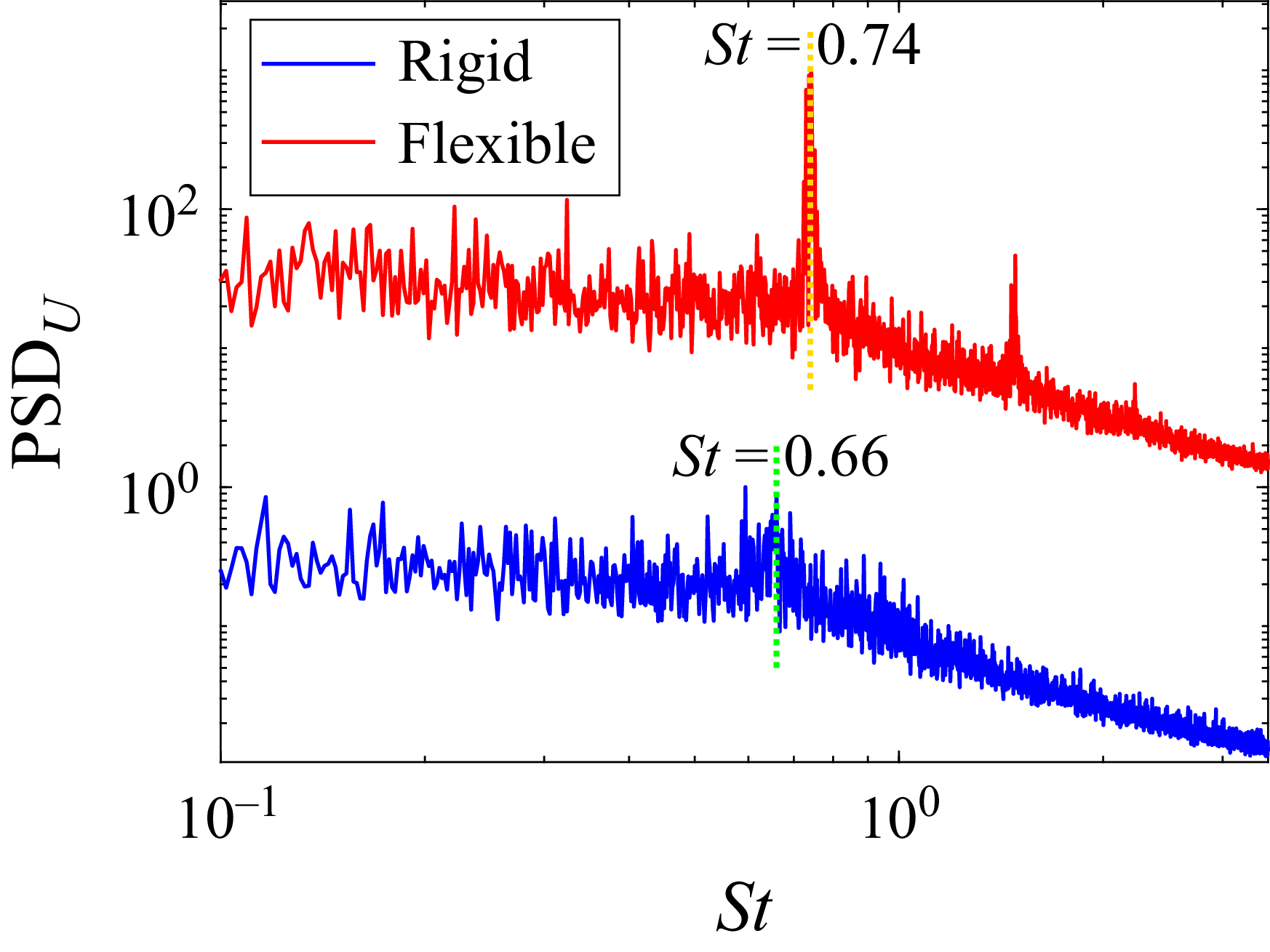
 α=13∘


 α=0∘
 13∘
 Δt=0
 Δt=−1/4T
 −1/2T
 π/2
 π

 α=19∘


 α=13∘
 a2
 ψ1
 ±1

 α=10∘
 α=13∘

 α=10∘
 α=13∘

 α=10∘
 α=13∘

 α=10∘
 α=13∘

 α=10∘
 α=13∘

 α=13∘


