1. Introduction
A jet in crossflow (also referred to as a transverse jet) describes a jet of fluid that exits an orifice and interacts with fluid flowing in a direction perpendicular to the jet. Jets in crossflow occur in a wide range of practical applications – dilution air jets in combustors, fuel injectors, thrust vectoring and V/STOL aircraft. Jets in crossflow have been studied for a number of years, both experimentally and computationally. Much of this work may be found in the reviews by Margason (Reference Margason1993), Karagozian (Reference Karagozian2010) and Mahesh (Reference Mahesh2013). The fundamental dynamics of the jet in crossflow involve an inter-related set of vortex systems, including upstream shear layer vortices, the counter-rotating vortex pair (CVP) observed to dominate the jet cross-section (Kamotani & Greber Reference Kamotani and Greber1972; Smith & Mungal Reference Smith and Mungal1998), horseshoe vortices which form in the plane of the flush jet’s injection wall (Kelso & Smits Reference Kelso and Smits1995) and upright wake vortices (Fric & Roshko Reference Fric and Roshko1994).
Instabilities associated with the transverse jet’s upstream shear layer are of considerable importance to transverse jet control. Yet, until recently, there have been few studies that have quantified Strouhal numbers associated with transverse jet shear layer instabilities for a range of conditions. The velocity ratio (
 $R=\overline{v}_{j}/u_{\infty }$
) defined as the ratio of the jet to crossflow velocity is used to characterize a jet in crossflow. The experiments of Megerian et al. (Reference Megerian, Davitian, Alves and Karagozian2007) and Davitian et al. (Reference Davitian, Getsinger, Hendrickson and Karagozian2010) explore the range
 $1.15\leqslant R<\infty$
, at fixed jet Reynolds numbers (2000 and 3000). In the parameter range
 $3.2<R<\infty$
, dominant shear layer instabilities are observed through measured spectra to be strengthened, to move closer to the jet orifice, and to increase in frequency as crossflow velocity
 $U_{\infty }$
increases for a fixed jet Reynolds number
 $Re$
.
The shear layer instabilities at higher
 $R$
values (above 3.2) exhibit frequency shifting downstream along the jet shear layer. When
 $R$
is reduced below approximately 3.2, single frequency instabilities are dramatically strengthened, forming almost immediately beyond the jet exit within the shear layer, without any evidence of frequency shifting. The spectra along the jet shear layer for
 $R>3.2$
are typical of convectively unstable shear layers where disturbances grow downstream of their initiation (Huerre & Monkewitz Reference Huerre and Monkewitz1990), while the spectra for
 $R<3.2$
are typical of an absolutely unstable shear flow where disturbances also grow near their location of initiation. As a result, the flow becomes self-excited. While a number of canonical flows are known to become absolutely unstable under certain critical conditions, Megerian et al. (Reference Megerian, Davitian, Alves and Karagozian2007) appear to be the first to have discovered such a transition in the transverse jet. The difference in shear layer behaviour corresponds to a difference in how the jet responds to axial forcing; strong square wave forcing is necessary at low velocity ratios while small amplitude sinusoidal pulsing is found effective at higher velocity ratios.
Bagheri et al. (Reference Bagheri, Schlatter, Schmid and Henningson2009) performed a global stability analysis of a jet in crossflow at a velocity ratio of 3 and found multiple unstable modes. The most unstable mode corresponded to loop-shaped vortical structures on the jet shear layer while lower frequency unstable modes were associated with the wake of the jet in the boundary layer. A steady base flow was used for the global stability analysis. Rowley et al. (Reference Rowley, Mezic, Bagheri, Schlatter and Henningson2009) performed a Koopman mode analysis (also referred to as dynamic mode decomposition (DMD)) of a jet in crossflow at the same conditions as Bagheri et al. (Reference Bagheri, Schlatter, Schmid and Henningson2009) and showed that the Koopman modes capture the dominant frequencies associated with the flow. The simulations by both Bagheri et al. (Reference Bagheri, Schlatter, Schmid and Henningson2009) and Rowley et al. (Reference Rowley, Mezic, Bagheri, Schlatter and Henningson2009) used a prescribed parabolic velocity profile at the jet exit and neglected the effects of a nozzle or pipe. Schlatter, Bagheri & Henningson (Reference Schlatter, Bagheri and Henningson2011) found that neither the inclusion of the jet pipe nor unsteadiness are necessary to generate the characteristic counter-rotating vortex pair. While these numerical studies yield important insights, they do not address the influence of nozzle on shear layer instability.
This paper uses DNS to study this phenomenon of instability transition with velocity ratio. To the best of our knowledge, this behaviour has not yet been computationally reproduced nor has a physical mechanism been proposed. This paper attempts to address these issues. We simulate two flow conditions:
 $R=2$
and
 $R=4$
at a jet
 $Re=2000$
which match the experimental conditions of Megerian et al. (Reference Megerian, Davitian, Alves and Karagozian2007). The simulations include the nozzle used in the experiments, and are compared to experimental data. DMD or Koopman mode decomposition (Rowley et al.
Reference Rowley, Mezic, Bagheri, Schlatter and Henningson2009; Schmid Reference Schmid2010) is then used to better understand the difference in the flow characteristics between low and high values of
 $R$
. This paper also quantifies the effect of simulating a nozzle by prescribing the same mean flow field obtained from the simulation with nozzle for
 $R=2$
. Also, the effect of varying the jet exit shear layer thickness is studied by prescribing a pipe-like profile at the jet exit and comparing the nature of the shear layer instability to the simulation with a nozzle.
This paper is organized as follows. Section 2 briefly describes the algorithm used in the DNS and DMD. Section 3 describes the flow conditions and relevant computational details. The numerical results are compared to those from experiments in § 4. The comparison includes shear layer velocity spectra, mean velocity contours and mean streamlines. Section 5 discusses in detail the results from DNS and DMD for
 $R=2$
and 4 which correspond to the simulations that match the experiments of Megerian et al. (Reference Megerian, Davitian, Alves and Karagozian2007). Section 6 quantifies the effect of simulating the nozzle for
 $R=2$
. The effect of jet exit velocity on the shear layer characteristics is discussed in § 7 by comparing the results of
 $R=2$
flow to simulations with a prescribed pipe-like jet exit velocity. Finally, § 8 summarizes the main findings of the paper.
2. Numerical algorithm
2.1. Direct numerical simulation
The simulations use an unstructured grid, finite-volume algorithm developed by Mahesh, Constantinescu & Moin (Reference Mahesh, Constantinescu and Moin2004) for solving the incompressible Navier–Stokes equations. The algorithm emphasizes discrete kinetic energy conservation in the inviscid limit which enables it to simulate high Reynolds number flows in complex geometries without adding numerical dissipation. Least-square reconstruction is used for the viscous terms and an explicit second-order Adams–Bashforth scheme is used for time integration. The solution is advanced using a predictor–corrector methodology where the velocities are first predicted using the momentum equation alone, and then corrected using the pressure gradient obtained from the Poisson equation yielded by the continuity equation. The algorithm has been validated for a wide range of complex problems which include a gas turbine combustor geometry (Mahesh et al. Reference Mahesh, Constantinescu and Moin2004) and predicting propeller crashback (Verma, Jang & Mahesh Reference Verma, Jang and Mahesh2012; Jang & Mahesh Reference Jang and Mahesh2013). It has been used to study the entrainment from free jets by (Babu & Mahesh Reference Babu and Mahesh2004) and was applied to transverse jets by Muppidi & Mahesh (Reference Muppidi and Mahesh2005, Reference Muppidi and Mahesh2007, Reference Muppidi and Mahesh2008) and Sau & Mahesh (Reference Sau and Mahesh2007, Reference Sau and Mahesh2008). DNS of a round turbulent jet in crossflow was performed by Muppidi & Mahesh (Reference Muppidi and Mahesh2007) under the same conditions as Su & Mungal’s (Reference Su and Mungal2004) experiments, and very good agreement with the experimental data was obtained. DNS of passive scalar mixing was performed under the same conditions as experiment by Muppidi & Mahesh (Reference Muppidi and Mahesh2008) and used to examine the entrainment mechanisms of the transverse jet.
2.2. Dynamic mode decomposition
We follow the method of Rowley et al. (Reference Rowley, Mezic, Bagheri, Schlatter and Henningson2009) and Schmid (Reference Schmid2010) to perform DMD (also referred to as Koopman mode decomposition) of the three-dimensional flow field for
 $R=2$
and 4. We store (
 $m+1$
) snapshots of the three velocity components at each spatial location and express the last snapshot as a linear combination of the previous snapshots. The size of each
 $x_{i}$
vector is the number of grid points multiplied by the number of velocity components. The size of each vector for the jet in crossflow problem is
 $80~\text{million}\times 3=240~\text{million}$
. Let
 $\unicode[STIX]{x1D646}$
represent a matrix of the different snapshots from
 $x_{0}$
to
 $x_{m-1}$
,
 $$\begin{eqnarray}\displaystyle \unicode[STIX]{x1D646}=[x_{0},x_{1},x_{2},\ldots ,x_{m-1}]. & & \displaystyle\end{eqnarray}$$
Suppose each snapshot (
 $x_{i}$
) is obtained from application of a linear matrix
 $\unicode[STIX]{x1D63C}$
to the previous snapshot (
 $x_{i-1}$
), the matrix
 $\unicode[STIX]{x1D646}$
can also be written as:
 $$\begin{eqnarray}\displaystyle \unicode[STIX]{x1D646}=[x_{0},\unicode[STIX]{x1D63C}x_{0},\unicode[STIX]{x1D63C}^{2}x_{0},\ldots ,\unicode[STIX]{x1D63C}^{m-1}x_{m-1}]. & & \displaystyle\end{eqnarray}$$
Now, expressing the last snapshot (
 $x_{m}$
) as a linear combination of the previous snapshots,
 $$\begin{eqnarray}\displaystyle x_{m}=c_{0}x_{0}+c_{1}x_{1}+c_{2}x_{2}+\cdots c_{m-1}x_{m-1}+r=Kc+r. & & \displaystyle\end{eqnarray}$$
In the above equation,
 $r$
represents the residual of the linear combination. If the residual is zero, then the above representation would be exact. Here,
 $\boldsymbol{c}$
is given by:
 $$\begin{eqnarray}\displaystyle \boldsymbol{c}=(c_{0},c_{1},c_{2},\ldots ,c_{m-1})^{\text{T}}. & & \displaystyle\end{eqnarray}$$
The vector
 $\boldsymbol{c}$
is obtained by solving the least-squares problem in (2.3) using singular value decomposition (SVD). Based on the above definitions, we obtain:
 $$\begin{eqnarray}\displaystyle \unicode[STIX]{x1D63C}\unicode[STIX]{x1D646}=\unicode[STIX]{x1D646}\unicode[STIX]{x1D63E}+r\text{e}^{\text{T}},\quad \text{e}^{\text{T}}=(0,0,\ldots ,1), & & \displaystyle\end{eqnarray}$$
where
 $\unicode[STIX]{x1D63E}$
is a companion matrix whose eigenvalues approximate those of the matrix
 $\unicode[STIX]{x1D63C}$
, which represents the dynamics of the flow. The imaginary part of the eigenvalue gives the frequency while the real part gives the growth rate of the mode. The eigenvector (
 $\boldsymbol{v}$
) or the spatial variation of the DMD mode is obtained from the eigenvector of the companion matrix (
 $\unicode[STIX]{x1D63E}$
) and the matrix (
 $\unicode[STIX]{x1D646}$
). The energy of each DMD mode is the L2-norm of the eigenvector
 $\boldsymbol{v}$
. Here, the vectors
 $x_{i}$
are obtained by the operation of the nonlinear Navier–Stokes operator and the eigenvalues and eigenvectors approximate the Koopman modes of the dynamical system. The reader is referred to Rowley et al. (Reference Rowley, Mezic, Bagheri, Schlatter and Henningson2009) and Schmid (Reference Schmid2010) for further theoretical and implementation details.
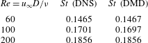
We perform DMD for two-dimensional cylinder flow at Reynolds numbers (
 $Re=u_{\infty }D/{\it\nu}$
) of 60, 100 and 200 to validate the method. The computational grid has 1 million elements and the upstream, downstream and spanwise extents (on either side of the centre plane) are 20, 40 and 50 respectively when scaled with the cylinder diameter (
 $d$
). The size of each vector for the DMD is
 $1~\text{million}\times 2=2~\text{million}$
. The Strouhal number (
 $St=fd/u_{\infty }$
) computed from the time history of lift in the DNS is compared to the
 $St$
obtained from DMD (of the most energetic mode) in table 1. Note that the agreement is excellent, thus validating the DMD methodology. Also, the values of
 $St$
obtained are in agreement with past studies (Tritton Reference Tritton1959). Here, 50 snapshots were used in the DMD computation with a
 ${\rm\Delta}tu_{\infty }/D=0.4$
. The vorticity contours of the most energetic DMD mode (not shown) for
 $Re=60$
was qualitatively similar to those obtained by Chen, Tu & Rowley (Reference Chen, Tu and Rowley2012) at the same
 $Re$
and the streamfunction contours by Bagheri (Reference Bagheri2013) at
 $Re=50$
.
3. Problem description
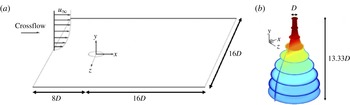
A schematic of the problem is shown in (a) and shape of the nozzle coloured by vertical velocity contours in (b). The vertical extent of the domain is
 $16D$
.

Validation of DMD for a 2-D cylinder. The
 $St$
from DNS is obtained from the lift spectra.

A schematic of the problem is shown in figure 1. A laminar boundary layer crossflow is prescribed at the inflow of the computational domain, and the jet emanates out of the origin in the figure. For the simulations with nozzle, its shape is modelled by a fifth-order polynomial (figure 1) and matches the nozzle used in the experiments of Megerian et al. (Reference Megerian, Davitian, Alves and Karagozian2007). The diameter of the jet nozzle (
 $D$
) at the exit is 3.81 mm and the mean velocity of the jet (
 $\overline{v}_{j}$
) is
 $8~\text{m}~\text{s}^{-1}$
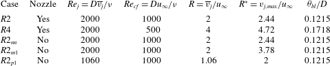
. The simulation conditions are listed in table 2. The simulation conditions
 $R2$
and
 $R4$
match the experimental conditions of Megerian et al. (Reference Megerian, Davitian, Alves and Karagozian2007) corresponding to velocity ratios (
 $R=\overline{v}_{j}/u_{\infty }$
) of 2 and 4. Here
 $u_{\infty }$
denotes the free-stream velocity of the crossflow. To assess the effect of simulating the nozzle for
 $R2$
,
 $R2_{nn}$
was performed without the nozzle where a steady jet exit profile was prescribed from the mean flow field of the
 $R2$
simulation.
 $R2_{m1}$
and
 $R2_{p1}$
correspond to simulations without the nozzle and a pipe-like steady profile imposed at the jet exit to study the effect of varying the jet exit profile on the shear layer instability.
 $R2_{m1}$
and
 $R2_{p1}$
have a mean and peak jet velocity of 1 respectively. Further details of
 $R2_{nn}$
,
 $R2_{m1}$
and
 $R2_{p1}$
are discussed in §§ 6 and 7.
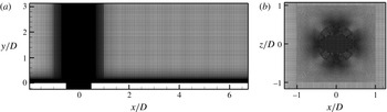
The grid used in the simulation is shown in (a) symmetry plane and (b) wall-parallel view close to jet exit. Note that the grid is finer in the vicinity of the jet.

Table listing the flow conditions used in the study.
 $R2$
and
 $R4$
correspond to the experimental conditions of Megerian et al. (Reference Megerian, Davitian, Alves and Karagozian2007).
 $R2_{nn}$
corresponds to the simulation similar to
 $R2$
but without simulating a nozzle and prescribing the jet exit velocity from the
 $R2$
simulation.
 $R2_{m1}$
and
 $R2_{p1}$
correspond to the simulations without the nozzle with a pipe-like prescribed jet exit velocity profile.
 $R2_{m1}$
has a mean jet exit velocity of 1 and
 $R2_{p1}$
has a peak jet exit velocity of 1. Here,
 ${\it\theta}_{bl}$
is the momentum thickness of the crossflow boundary layer at the jet exit location when the jet is turned off.

The unstructured grid capability enables simulation of the flow inside the nozzle along with the crossflow domain. The inflow, outflow, top wall and side walls of the computational domain are located at 8
 $D$
, 16
 $D$
, 16
 $D$
and 8
 $D$
from the origin respectively as shown in the schematic in figure 1. Zero-gradient Neumann boundary conditions are specified at the outflow and side walls, while the inflow boundary condition is prescribed as a laminar boundary layer obtained from the Blasius similarity solution. A view of the symmetry plane and a top view of the grid are shown in figure 2. A coarse and fine grid containing 10 and 80 million grid points respectively were used in this study. Details of the 80 million grid are described here. There are 400 points along the circumference of the jet exit. The upstream portion of the grid contained 80 points within the boundary layer in the
 $y$
-direction. A constant spacing of
 ${\rm\Delta}x/D=0.033$
and
 ${\rm\Delta}z/D=0.02$
was maintained downstream of the jet with a
 ${\rm\Delta}y_{min}/D=0.0013$
. The spacings used are finer than those used by Muppidi & Mahesh (Reference Muppidi and Mahesh2007) for a turbulent jet in crossflow. Assuming that the boundary layer downstream was turbulent at the outflow, this yields viscous wall spacings
 ${\rm\Delta}y_{min}^{+}/D$
,
 ${\rm\Delta}x^{+}/D$
and
 ${\rm\Delta}z^{+}/D$
of 0.1, 2.74 and 1.66 for
 $R=2$
and 0.058, 1.48 and 0.89 for
 $R=4$
respectively. The viscous spacings were computed assuming
 $c_{f}=0.0576Re_{x}^{-0.2}$
for a turbulent boundary layer (Schlichting Reference Schlichting1968).
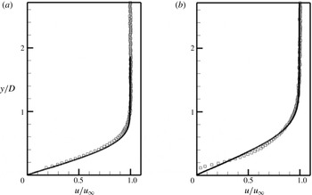
Streamwise velocity profiles from simulation (——) and experiment (▫) (A. R. Karagozian, personal communication, 2012) at
 $x/D=-5.5$
from the jet exit for
 $R=2$
(a) and
 $R=4$
(b).

To prescribe the Blasius boundary layer similarity solution at the inflow, the profiles were compared to those obtained from the experiment with the jet turned off (A. R. Karagozian, private communication, 2012). The inflow solution was prescribed so as to match the experimental profiles at 5.5
 $D$
upstream of the jet inflow location. Figure 3 shows the streamwise velocity obtained from the simulation with the jet turned on and the velocity profiles obtained from the experiment for
 $R=2$
and 4. Overall, we see good agreement with experiment. From figure 3, it can be seen that the boundary layer is thicker for
 $R=4$
due to the lower crossflow Reynolds number as also indicated by the momentum thickness (
 ${\it\theta}_{bl}/D$
) values of 0.1215 and 0.1718 (listed in table 2) for
 $R=2$
and 4, respectively. Note that there are minor deviations between the experimental and Blasius profiles especially for the
 $R=4$
profile close to the wall.
4. Comparison to experiment
4.1. Upstream shear layer spectra
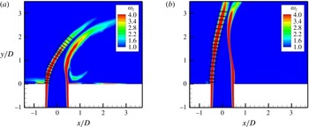
Instantaneous spanwise vorticity contours in the symmetry plane for
 $R=2$
(a) and
 $R=4$
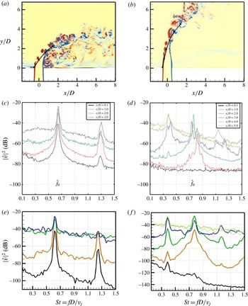
(b). The black dots indicate the locations at which velocity spectra are shown in the figures below. Vertical velocity spectra from experiments of Megerian et al. (Reference Megerian, Davitian, Alves and Karagozian2007) (c,d) and simulation (e,f) are shown. Plots of
 $R=2$
are on (a,c,e) while
 $R=4$
are on (b,d,f). The lines correspond to the distance (
 $s/D$
) from
 $(x/D,y/D)=(-0.5,0)$
with
 $s/D=0.1$
(black), 1 (orange), 2 (green), 3 (blue), 4 (grey) and 5 (purple). The spatial coordinates of the points are listed in the text.

Point velocity spectra were obtained at various locations in the flow. Figure 4 compares the vertical velocity spectra (scaled by the mean jet exit velocity) obtained from the simulation to those obtained from the experiment at different stations along the shear layer (
 $s/D$
, where
 $s$
denotes the distance from the leading edge of the jet exit,
 $x/D,y/D=-0.5$
, 0) in the symmetry plane (
 $z=0$
). The spatial locations at which spectra are shown in figure 4 correspond to (
 $x/D$
,
 $y/D$
) of (
 $-0.5$
, 0.1), (0.006, 0.854), (0.654, 1.614) and (1.432, 2.238) for
 $R=2$
and (
 $-0.5$
, 0.1), (
 $-0.329$
, 0.958), (
 $-0.092$
, 1.933), (0.23, 2.873), (0.71, 3.75) and (1.38, 4.49) for
 $R=4$
. Here, the non-dimensional frequency or Strouhal number (
 $St=fD/v_{j}$
) is defined based on the diameter (
 $D$
) and peak velocity (
 $v_{j}$
) at the jet exit. The spectra were computed using 50 % overlap of the samples with 11 windows and a Hamming windowing function. The minimum
 $St$
from the spectra is 0.019 for both
 $R=2$
and 4 which is more than an order of magnitude lower than the dominant frequencies in the flow. Also shown are vorticity contours in the symmetry plane along with the spatial locations where the spectra are compared. Due to minor differences between the simulation and experiment in the boundary layer velocity profile upstream of the jet (figure 3) and mean jet exit velocity profile (figure 5), an exact quantitative match is not expected in the spectra. Hence, the spectra from experiment and simulation are shown in separate plots. Note that good agreement is observed between simulation and experiment. The velocity spectra from the coarse grid (not shown) which is coarser by a factor of 2 in each direction matched well with the experiment for
 $R=2$
but not for
 $R=4$
.
For the
 $R=2$
flow, it can be seen that
 $St=0.65$
is the most dominant along all the locations considered. However, for
 $R=4$
, it can been seen that at
 $s/d=0.1$
,
 $St=0.39$
is the most dominant, while further downstream,
 $St=0.78$
is most dominant, and far downstream at
 $s/d=5$
,
 $St=0.39$
is again most dominant. Thus, we observe that while a single frequency dominates for
 $R=2$
, different frequencies are dominant for
 $R=4$
flow. This phenomena has been extensively studied by Megerian et al. (Reference Megerian, Davitian, Alves and Karagozian2007), who found that the shear layer was absolutely unstable for
 $R<3.1$
giving rise to a single global frequency that was dominant throughout the shear layer while for
 $R>$
3.1, the shear layer was found to be convectively unstable leading to multiple frequencies being dominant along the shear layer. For
 $R=4$
, note that the
 $St=0.39$
peak is observed at all points in the DNS but not at the first couple of locations in the experiment, possibly due to the very low amplitude of the peak.
The instantaneous vorticity contours depict a clear roll up of the leading-edge shear layer for both
 $R=2$
and 4. However, for
 $R=4$
, coherent roll up of the trailing edge is also visible which is not the case for
 $R=2$
. It can also be observed that vortical activity exists between the jet and the wall for
 $R=2$
but not for
 $R=4$
indicating a stronger jet–wall interaction at lower velocity ratios.
4.2. Mean velocity and streamlines
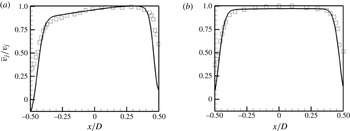
Mean vertical velocity profiles from simulation (——) and experiments of Megerian et al. (Reference Megerian, Davitian, Alves and Karagozian2007) (▫) in the symmetry plane at
 $y/D=0.1$
from the flat plate for
 $R=2$
(a) and
 $R=4$
(b).

Figure 5 shows the mean vertical velocity profiles from the simulation and experiment at
 $y/D=0.1$
in the symmetry plane for
 $R=2$
and 4. Overall, good agreement is observed except in the vicinity of the jet wall. We see that the
 $R=2$
flow is more asymmetric when compared to
 $R=4$
indicating the greater effect of the crossflow on the jet for
 $R=2$
. We also see from the simulation results for
 $R=2$
that there is a region of reverse flow close to the jet exit indicating a higher adverse pressure gradient created by the crossflow.
Mean streamwise velocity contours in the symmetry plane are shown for
 $R=2$
(a–c) and
 $R=4$
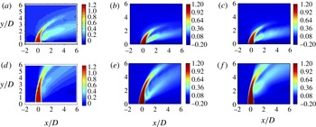
(d–f). Figures from experiments of Getsinger (Reference Getsinger2012) (a,d), coarse grid DNS (b,e) and fine grid DNS (c,f) are shown for comparison. Note that the experimental figures (a,d) correspond to
 $R=2.2$
and 4.4, respectively.

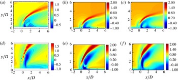
Mean vertical velocity contours in the symmetry plane are shown for
 $R=2$
(a–c) and
 $R=4$
(d–f). Figures from experiments of Getsinger (Reference Getsinger2012) (a,d), coarse grid DNS (b,e) and fine grid DNS (c,f) are shown for comparison. Note that the experimental figures (a,d) correspond to
 $R=2.2$
and 4.4, respectively.

Figure 6 shows contours of the mean streamwise velocity for
 $R=2$
and 4 from the coarse and fine grid simulations and compares it to the experiments of Getsinger (Reference Getsinger2012) at similar conditions of
 $R=2.2$
and 4.4. Overall, good agreement is observed. However, the jet trajectory in the simulations is slightly shallower when compared to the experiments due to the higher velocity ratio of the experiments. The
 $R=2$
jet is closer to the flat plate when compared to
 $R=4$
due to the lower momentum of the jet at
 $R=2$
. Figure 7 shows the mean vertical velocity contours for
 $R=2$
and 4 from the coarse and fine grid simulations and compares it to the experiments of Getsinger (Reference Getsinger2012) at similar conditions of
 $R=2.2$
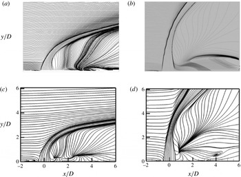
and 4.4. Good agreement is observed between simulation and experiment. Figure 8 compares the mean streamlines obtained from experiment to those obtained from the fine grid simulations for
 $R=2$
and 4. Again, good agreement is observed between experiment and simulation. For
 $R=2$
, upstream of the jet, a prominent boundary layer separation vortex is visible which is absent for
 $R=4$
. Downstream of the jet, nodes are observed in the streamlines in the symmetry plane (
 $z=0$
) indicating that the fluid is being entrained into the plane due to the crossflow fluid going around the jet. Such a node downstream of the jet has also been observed by other researchers such as Kelso, Lim & Perry (Reference Kelso, Lim and Perry1996), Muppidi & Mahesh (Reference Muppidi and Mahesh2005) and Schlatter et al. (Reference Schlatter, Bagheri and Henningson2011). While a single node is observed for
 $R=4$
, similar to Kelso et al. (Reference Kelso, Lim and Perry1996) and Muppidi & Mahesh (Reference Muppidi and Mahesh2005); an additional node closer to the jet is observed for
 $R=2$
which was also observed by Schlatter et al. (Reference Schlatter, Bagheri and Henningson2011). A more intense low pressure region is observed downstream of the jet for
 $R=2$
as compared to
 $R=4$
as can be seen in the instantaneous pressure contours shown in figure 11.
Mean streamlines in the symmetry plane from experiment (a,b) (A. R. Karagozian, personal communication, 2012) and simulation (c,d) for
 $R=2$
(a,c) and
 $R=4$
(b,d).

5. Effect of velocity ratio
The results of
 $R2$
and
 $R4$
which correspond to the experimental conditions of Megerian et al. (Reference Megerian, Davitian, Alves and Karagozian2007) are discussed in this section. A detailed investigation of the instantaneous and mean flow fields from DNS and data extracted from DMD is performed to understand the difference in the absolute versus convective nature of the upstream shear layer instability for the two flows. Note that the nozzle is included in the simulations here.
 $R2$
and
 $R4$
flow conditions are also referred to as
 $R=2$
and
 $R=4$
respectively in this section.
5.1. Instantaneous flow features
Instantaneous isocontours of
 $Q$
coloured by streamwise velocity contours for
 $R=2$
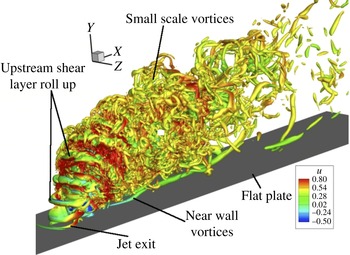
. Note the coherent shear layer roll up and small scale features further downstream.

Instantaneous isocontours of
 $Q$
coloured by streamwise velocity contours for
 $R=4$
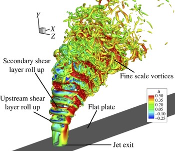
. Note the coherent shear layer roll up and small scale features further downstream.

Figure 9 shows isocontours of
 $Q$
coloured by streamwise velocity contours for
 $R=2$
, where
 $Q$
is defined as follows (Hunt, Wray & Moin Reference Hunt, Wray and Moin1988):
 $Q=-0.5((\text{d}u_{i}/\text{d}x_{j})(\text{d}u_{j}/\text{d}x_{i}))$
. In an incompressible flow, the
 $Q$
-criterion represents regions of pressure minimum which occurs in vortex cores. From the divergence of the Navier–Stokes equations,
 $Q=-{\rm\Delta}p$
where
 ${\rm\Delta}$
is the Laplacian operator. Thus, regions of negative
 $Q$
represent pressure minima which are used to identify vortex cores. The
 $Q$
-criterion can be used to identify any coherent vortex whether it lies in the jet shear layer or wake and does not differentiate between the two regions. Note the roll up of the shear layer near the jet exit along the jet trajectory, followed by smaller scale vortices indicating the transitional/turbulent nature of the flow. Also visible are long vortices close to the wall. Figure 10 shows isocontours of
 $Q$
coloured by streamwise velocity for
 $R=4$
. Again, the shear layer roll up is clearly visible followed by smaller scale vortices along the jet trajectory. Note that the roll up takes place farther away from the wall when compared to
 $R=2$
and that vortices are absent close to the wall. A closer look at the
 $R=4$
isocontours reveals secondary roll-up vortices that are smaller in size and are due to the roll up of the trailing edge shear layer. Such vortices are not very prominent for
 $R=2$
. Also, vortices can be observed close to the wall for
 $R=2$
due to the interaction between the jet and the wall which is not seen for
 $R=4$
.
Instantaneous pressure contours (
 $p/{\it\rho}\overline{v}_{j}^{2}$
) with streamlines are shown in the symmetry plane for
 $R=2$
(a) and
 $R=4$
(b).

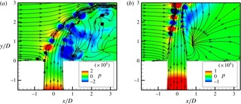
Figure 11 shows instantaneous pressure contours along with streamlines in the symmetry plane for
 $R=2$
and 4. The roll up of the shear layer is clearly visible for both the flows with the roll up occurring close to the jet exit for
 $R=2$
. Upstream of the jet, a boundary layer separation vortex is visible for
 $R=2$
, which is absent for
 $R=4$
. The roll up of the shear layer extends into the nozzle for
 $R=2$
. This can be explained by the fact that the flow inside nozzle separates close to the jet exit for
 $R=2$
due to the higher momentum of the crossflow when compared to
 $R=4$
. This causes the shear layer to be stronger for
 $R=2$
close to the exit, causing it to become unstable and roll up. Also, there is a large low pressure region downstream of the jet for
 $R=2$
along with a recirculation vortex which is absent for the
 $R=4$
jet. There is a source point located downstream of the jet for both flows caused by the reattachment of the crossflow streamlines in the plane parallel to the wall. The source point is located farther from the jet for
 $R=2$
.
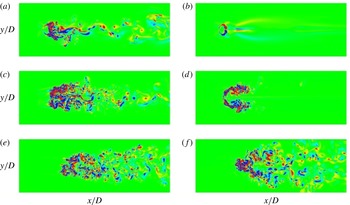
Instantaneous wall-normal vorticity contours (
 ${\it\omega}_{y}$
) are shown in planes parallel to the wall for
 $R=2$
and 4 at three different locations to quantify the nature of the wake caused by the jet. At the location closest to the wall (
 $y/D=0.67$
), for
 $R=2$
, the wake appears to be asymmetric and unsteady. However, for
 $R=4$
, at the location closest to the wall (
 $y/D=1.3$
), the wake appears to be quiescent. A lower crossflow Reynolds number for
 $R=4$
and the delay in shear layer roll up as observed in figure 4 due to the higher momentum of the jet are likely responsible for the quiescent nature of the wake for
 $R=4$
. At the farthest location from the wall shown in figure 12, for both flows, smaller scales are observed at large distances downstream of the jet exit, indicating the transitional/turbulent nature of the jet.
Instantaneous wall-normal vorticity contours (
 ${\it\omega}_{y}$
) are shown at (a)
 $y/D=0.67$
, (c)
 $y/D=1.3$
and (e)
 $y/D=3.33$
for
 $R=2$
and (a)
 $y/D=1.3$
,(c)
 $y/D=3.33$
and (e)
 $y/D=6.67$
for
 $R=4$
.

Temporal variation of
 $u$
(blue line),
 $v$
(green line) and
 $w$
(red line) velocities along the leading-edge shear layer in the symmetry plane (
 $z=0$
) for
 $R=2$
at (
 $x/D=0.006,y/D=0.854$
) (a) and
 $R=4$
at (
 $x/D=-0.092,y/D=1.933$
) (b) where
 $D/L=0.15$
. Note that a lower frequency is observed in the
 $w$
velocity for
 $R=2$
.

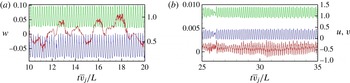
For
 $R=2$
, there exists a region of low pressure downstream of the jet (figure 11) and an asymmetric, unsteady wake (figure 12). Also, in figure 4, only the vertical velocity spectra along the upstream shear layer was discussed. We plot the variation of
 $u$
,
 $v$
and
 $w$
velocities with time at
 $s/D=0.1$
(for
 $R=2$
) and at
 $s/D=0.2$
for
 $R=4$
in figure 13, where
 $s/D$
is defined along the leading-edge shear layer as in figure 4. While the same frequency is dominant for
 $R=4$
in all the three velocity spectra, it can be seen that a very low frequency is dominant in the
 $w$
velocity for
 $R=2$
. From figure 13, the Strouhal number based on the crossflow velocity and diameter of the jet exit (
 $St_{c}=u_{\infty }D/{\it\nu}$
) corresponding to the low frequency in
 $w$
velocity for
 $R=2$
is approximately 0.15 which is close to the values of 0.15–0.17 reported by Kelso et al. (Reference Kelso, Lim and Perry1996) in the wake of a jet in crossflow at the same
 $R$
. This indicates that the frequency is related to the wake phenomena for
 $R=2$
as seen in figures 11 and 12.
5.2. Mean comparisons
Mean pressure contours (
 $p/{\it\rho}\overline{v}_{j}^{2}$
) are shown in the symmetry plane for
 $R=2$
(a) and
 $R=4$
(b). Note that the colour scale is different between the two figures to emphasize the differences in the flow field.

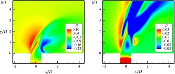
Figure 14 shows the mean pressure contours in the symmetry plane for
 $R=2$
and 4. A high pressure region upstream of the jet is observed similar to Muppidi & Mahesh (Reference Muppidi and Mahesh2005). Also, a region of low pressure in the upstream shear layer lies between regions of high pressure on either side and corresponds to the location of the shear layer roll up. For
 $R=4$
, it can be seen that this low pressure region lies further away from the wall as compared to
 $R=2$
flow. It can be observed that the pressure field varies significantly as
 $R$
is varied. While the region of minimum pressure occurs downstream of the jet close to the downstream shear layer for
 $R=2$
, the same occurs along the jet trajectory for
 $R=4$
. Also, the region of low pressure occurs close to the wall for
 $R=2$
which is not the case for
 $R=4$
. Since the region of low pressure occurs downstream of the jet closer to the wall for
 $R=2$
, it is due to the obstruction of the boundary layer by the jet, while for
 $R=4$
, the low pressure region is due to the turning of the jet. Since the high pressure upstream of the jet occurs due to the obstruction of the crossflow by the jet, the magnitude would scale with the square of the crossflow velocity. Since the
 $R=2$
flow has a higher crossflow velocity (
 $u_{\infty }=0.5$
) as compared to
 $R=4$
(
 $u_{\infty }=0.25$
), the magnitude of high pressure would be large enough to cause the jet boundary layer to separate at the exit as observed in figure 11.
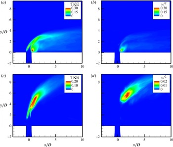
Figure 15 shows symmetry plane contours of turbulent kinetic energy (
 $\text{TKE}=\overline{u_{i}^{\prime }u_{i}^{\prime }}/u_{\infty }^{2}$
) and spanwise unsteadiness (
 $\overline{w^{\prime }w^{\prime }}/u_{\infty }^{2}$
) for
 $R=2$
and 4. For
 $R=2$
, it can be observed that the maximum unsteadiness occurs downstream of the jet close to the wall with a magnitude of
 ${\approx}\!0.3$
. Also,
 $\overline{w^{\prime }w^{\prime }}/u_{\infty }^{2}$
is predominant in the region of maximum TKE for
 $R=2$
with the magnitude being nearly equal to TKE downstream of the jet. This indicates a strong spanwise oscillation downstream of the jet for
 $R=2$
flow which is absent for
 $R=4$
. The region of maximum unsteadiness for
 $R=4$
occurs along the jet trajectory beyond
 $y/D=3.5$
.
Mean turbulent kinetic energy (TKE) (a,c) and
 $\overline{w^{\prime }w^{\prime }}$
contours (b,d) are shown in the symmetry plane for
 $R=2$
(a,b) and
 $R=4$
(c,d).

5.3. Shear layer dominance from DMD
DMD was performed for the entire three-dimensional flow field for
 $R=2$
and 4 using all the three velocity components (
 $u$
,
 $v$
,
 $w$
) using the algorithm described in § 2.2. The snapshots were taken at an interval of
 ${\rm\Delta}t\bar{v_{j}}/D=0.333$
units. Two hundred and forty-nine snapshots were used for
 $R=2$
while 80 snapshots were used for
 $R=4$
. For
 $R=2$
, the residual of the DMD approximation did not vary significantly between 100, 200 and 249 snapshots. Hence just 80 snapshots were used for
 $R=4$
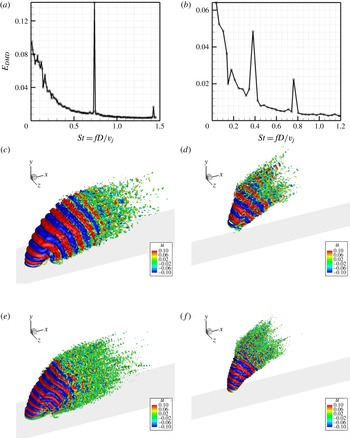
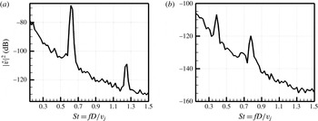
. Figure 16 shows the energy spectra of the DMD modes. Note the prominent peaks at
 $St=0.65$
and 1.3 for
 $R=2$
and
 $St=0.39$
and 0.78 for
 $R=4$
; they correspond to the same peaks observed along the shear layer. Thus, the shear layer modes are dominant global modes in the flow.
Spectral energy with Strouhal number obtained from DMD (a,b), isocontours of
 $Q$
obtained from DMD for
 $St=0.65$
(c),
 $St=0.39$
(d),
 $St=1.3$
(e) and
 $St=0.78$
(f). The plots correspond to
 $R=2$
(a,c,e) and
 $R=4$
(b,d,f) respectively.

Figure 16 shows the spatial DMD modes corresponding to the shear layer peaks using isocontours of
 $Q$
-criterion coloured with streamwise velocity contours (of the spatial DMD mode). Coherent three-dimensional shear layer vortices are observed for both
 $R=2$
and 4 corresponding to the roll up of the jet shear layer. The spatial modes corresponding to
 $St=1.3$
for
 $R=2$
and
 $St=0.78$
for
 $R=4$
display three-dimensional vortices with a smaller length scale suggestive of a harmonic. Note that the scale of the figure is different for
 $R=2$
and 4 to clearly depict the spatial mode. The vortices are coherent until a certain distance downstream, beyond which smaller scales can be observed.
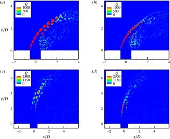
Symmetry plane contours of
 $Q$
criterion of the DMD mode for
 $St=0.65$
(a) and
 $St=1.3$
(b) for
 $R=2$
and
 $St=0.39$
(c) and
 $St=0.78$
(d) for
 $R=4$
.

Significant differences are observed between the spatial modes of
 $R=2$
and 4. For the
 $R=2$
jet, both the
 $St=0.65$
and 1.3 modes begin immediately at the flat plate (jet exit) whereas for
 $R=4$
, both the modes are located further away from the flat plate. Also, the
 $St=0.78$
mode lies closer to the flat plate for
 $R=4$
which explains why the
 $St=0.78$
mode is more dominant initially in figure 4 along the shear layer after which the
 $St=0.39$
mode becomes more dominant. It can also be observed from the spatial modes for
 $R=2$
that the shear layer vortices extend all the way up to the wall while no such behaviour is observed for
 $R=4$
modes. This indicates that the oscillation for
 $R=2$
is not just restricted to the shear layer, but is also present in the boundary layer downstream of the jet close to the wall.
To better understand the spatial DMD modes observed in figure 16, the symmetry plane contours of
 $Q$
criterion are shown in figure 17 for
 $R=2$
and 4. For
 $R=2$
, it can be observed that the upstream shear layer vortices are dominant for both
 $St=0.65$
and 1.3. Also, the spatial location of the modes coincide indicating that the
 $St=1.3$
is a higher harmonic of
 $St=0.65$
. For
 $R=4$
, while the upstream shear layer vortices are dominant for
 $St=0.78$
, the
 $St=0.39$
mode for
 $R=4$
is strongest closer to the centre of the jet beyond
 $y/D\approx 3.5$
, in contrast to the behaviour observed for
 $R=2$
.
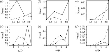
The magnitude of
 $u$
,
 $v$
and
 $w$
fluctuations obtained from DMD for
 $R=2$
(a–c) and
 $R=4$
(d–f) is shown along the upstream shear layer in the symmetry plane (
 $z=0$
). The velocity fluctuations are shown for
 $St=0.65$
(——) and 1.3 (– – –) for
 $R=2$
and
 $St=0.39$
(——) and 0.78 (– – –) for
 $R=4$
. The spatial locations are the same as those in figure 4 corresponding to
 $s/D=0.1$
, 1, 2, 3, 4 and 5 which are specified in § 4.1. Note that the locations at
 $s/D=4$
and 5 are only shown for
 $R=4$
.

From figure 4, we observed that while the
 $St=0.65$
mode was most dominant along the upstream shear layer for
 $R=2$
, initially
 $St=0.78$
was dominant for
 $R=4$
and further downstream,
 $St=0.39$
became most dominant indicative of a convective instability. Also, from figure 13, we saw that the dominant frequency of the
 $w$
velocity in the upstream shear layer for
 $R=2$
was different from the
 $St=0.65$
observed in the
 $v$
velocity spectra. Hence, we extract the magnitude of the fluctuation velocity components from DMD corresponding to the dominant frequencies observed from the
 $v$
velocity spectra. We extract magnitudes of velocity fluctuations corresponding to
 $St=0.65$
and 1.3 for
 $R=2$
and
 $St=0.39$
and 0.78 for
 $R=4$
. From the vertical velocity magnitude plots (figure 18
b,e), we observe that
 $St=0.65$
is always more dominant when compared to
 $St=1.3$
for
 $R=2$
while
 $St=0.78$
is more dominant until
 $s/D=4$
for
 $R=4$
beyond which
 $St=0.39$
becomes more dominant. These observations are consistent with those observed from figure 4 and the experiments of Megerian et al. (Reference Megerian, Davitian, Alves and Karagozian2007). While similar behaviour is observed for the
 $u$
fluctuation magnitude, the trend of
 $w$
fluctuation magnitude is very different. For
 $R=2$
,
 $St=1.3$
becomes more dominant than
 $St=0.65$
beyond
 $s/D=2.0$
while
 $St=0.78$
is always more dominant than
 $St=0.39$
for
 $R=4$
. It is also important to note that the magnitude of
 $w$
fluctuation is an order of magnitude smaller than
 $u$
and
 $v$
.
5.4. Analogy to counter-current mixing layer to explain absolute versus convective instability
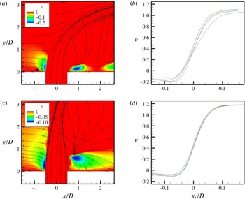
As the jet exits the nozzle and interacts with the crossflow boundary layer, the crossflow streamlines are deflected towards and away from the wall as they approach the jet which is shown in figure 20. This is similar to the streamline pattern obtained in front of an obstacle; see for example Baker (Reference Baker1979) and Simpson (Reference Simpson2001). Figure 20 shows the symmetry plane contours of the mean vertical velocity (
 $v$
) for
 $R=2$
and 4 with mean streamlines. Note that only regions of negative
 $v$
are shown in the figure. It can be seen that regions of negative
 $v$
are observed upstream and downstream of the jet. Note that the region upstream of the jet lies closer to the jet and occurs due to the streamlines below the stagnation streamlines deflected towards the wall due to the pressure difference.


Mean vertical velocity contours (a,c) are shown in the symmetry plane along with variation of mean vertical velocity along the upstream shear layer (b,d) for
 $R=2$
(a,b) and
 $R=4$
(c,d). The velocity profiles in (b,d) are taken in the region upstream of the jet where
 $v$
is negative and
 $x_{s}$
is the coordinate perpendicular to the upstream shear layer streamline. Note that the colour scale is different between the two figures to emphasize the differences in the flow field.

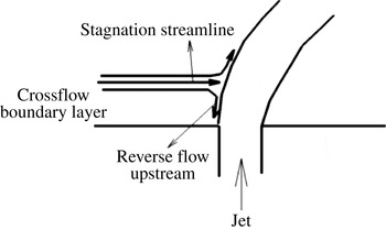
Schematic showing the stagnation streamline and reverse flow upstream for a jet in crossflow.

Figure 20 also shows the variation of mean vertical velocity (
 $v$
) at lines extracted along the upstream shear layer as shown in figure 19. Note that the profiles shown correspond to the region where
 $v$
is negative upstream of the jet. The profiles resemble a counter-current mixing layer where the sign of the velocity of the two streams are opposite. A mixing layer is characterized by its velocity ratio:
 $$\begin{eqnarray}\displaystyle R_{1}=\frac{V_{1}-V_{2}}{V_{1}+V_{2}}, & & \displaystyle\end{eqnarray}$$
where
 $V_{1}$
and
 $V_{2}$
are the velocity of the two streams, which are of opposite signs for a counter-current mixing layer yielding
 $R_{1}>$
1.
Huerre & Monkewitz (Reference Huerre and Monkewitz1985) used linear stability theory to theoretically predict that the counter-current mixing layer is absolutely unstable when
 $R_{1}>1.315$
while it is convectively unstable when
 $R_{1}<1.315$
. An absolutely unstable flow is characterized by a single frequency that is dominant throughout the flow while a convectively unstable flow can have multiple frequencies along the flow. This was verified by experiments of Strykowski & Niccum (Reference Strykowski and Niccum1991) who performed experiments for a round jet exiting a nozzle and suction was applied outside the nozzle to create a counter-current mixing layer profile. From their experiments, they found that a single frequency was dominant when the average
 $R_{1}$
was greater than 1.32 while multiple frequencies were dominant when
 $R_{1}$
was less than 1.32. Note that for a spatially evolving mixing layer,
 $R_{1}$
varies along the streamwise direction.
Since a similar transition from absolute to convective instability is observed for the jet in crossflow as we increase
 $R$
from 2 to 4 and a region of counter-current mixing layer is observed as shown in figure 20, we compute an equivalent mixing layer ratio (
 $R_{1}$
) for
 $R=2$
and 4 flows. Note that counter-current mixing layer profiles are obtained only in regions where there is a negative
 $v$
velocity upstream of the shear layer. The minimum mean
 $v$
velocity upstream of the shear layer (
 $V_{2}$
) is
 $-0.2$
and
 $-0.11$
for
 $R=2$
and 4 respectively from the simulations. From the velocity profiles in figures 20(b) and 20(d), we see that the maximum
 $v$
velocity (
 $V_{1}$
) is 1.1 and 1.2 for
 $R=2$
and 4, respectively. Corresponding to these values,
 $R_{1}$
is 1.44 and 1.2 for
 $R=2$
and 4, respectively. These values are clearly consistent with the absolute and convective instability behaviour of the counter-current mixing layers, suggesting that the mixing ratio in the upstream shear layer for a jet in crossflow is very important to the nature of the shear layer instability. Davitian et al. (Reference Davitian, Getsinger, Hendrickson and Karagozian2010) found that the transition from absolute to convective instability for a jet in crossflow occurs at
 $R_{critical}\approx 3$
and interpolating the value of mixing velocity ratio
 $R_{1}$
between the values of
 $R=2$
and 4 yields
 $R_{critical}=3$
corresponding to an
 $R_{1,critical}$
of 1.32 predicted by linear stability theory (Huerre & Monkewitz Reference Huerre and Monkewitz1985). Note that the value of 1.32 obtained by Huerre & Monkewitz (Reference Huerre and Monkewitz1985) is for a plane mixing layer. While the jet in crossflow interaction is three-dimensional and complex, with the presence of a curved shear layer and pressure gradient, it is interesting that the upstream mixing layer characteristics in the symmetry plane correlate with the instability behaviour of the jet–crossflow interaction.
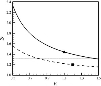
Variation of mixing layer velocity ratio
 $R_{1}=(V_{1}+V_{2})/(V_{1}-V_{2})$
with
 $V_{1}$
for
 $R=2$
(——) and 4 (– – –). A constant minimum mean upstream vertical velocity (
 $V_{2}$
) of
 $-0.2$
and
 $-0.11$
were chosen to compute
 $R_{1}$
for
 $R=2$
and 4 respectively.
 $R_{1}=1.32$
(
 $\cdots \cdots$
) represents the critical value beyond which the flow is absolutely unstable and ▴ and ▪ represent points corresponding to
 $R=2$
and 4, respectively.

Figure 21 shows a schematic of the jet in crossflow problem showing the stagnation streamline and the reverse region produced upstream of the jet shear layer. The pressure at the stagnation point (
 $P_{stag}$
) is given by:
 $$\begin{eqnarray}\displaystyle P_{stag}=P_{\infty }+{\textstyle \frac{1}{2}}{\it\rho}_{\infty }u_{\infty }^{2}, & & \displaystyle\end{eqnarray}$$
where
 $P_{\infty }$
,
 ${\it\rho}_{\infty }$
and
 $u_{\infty }$
are the free-stream crossflow pressure, density and velocity respectively. The velocity of the reverse flow (
 $v_{rev}$
) is given by:
 $$\begin{eqnarray}\displaystyle v_{rev}\approx \sqrt{\frac{1}{{\it\rho}}(P_{stag}-P_{wall})}. & & \displaystyle\end{eqnarray}$$
If we assume that the pressure at the wall (
 $P_{wall}$
) is of the order of
 $P_{\infty }$
, and since
 ${\it\rho}={\it\rho}_{\infty }$
, we get
 $$\begin{eqnarray}\displaystyle v_{rev}\approx ku_{\infty }, & & \displaystyle\end{eqnarray}$$
where
 $k$
is a constant. Thus, the magnitude of the reverse flow upstream of the shear layer depends on the velocity of the crossflow. This is consistent with the values of
 $-0.2$
and
 $-0.11$
obtained for
 $R=2$
and 4 respectively corresponding to a
 $u_{\infty }$
of 0.5 and 0.25. The value of
 $k$
is approximately
 $-0.4$
for both simulations. For a given crossflow velocity, to quantify the effect of increasing jet velocity, we plot the variation of
 $R_{1}$
with
 $V_{1}$
(velocity of the jet) in figure 22 for
 $R=2$
and 4 with
 $V_{2}=-0.2$
and
 $-0.11$
respectively. We also plot
 $R_{1}=1.32$
, which represents the critical value for transition from absolute to convectively unstable behaviour from the experiments of Strykowski & Niccum (Reference Strykowski and Niccum1991). It can be observed that with increasing jet velocity, the flow is likely to become more convectively unstable. Also, for a given jet velocity, increased crossflow velocity produces a higher magnitude of
 $V_{2}$
(from (5.4)), making the flow more absolutely unstable. From (5.1), a vertical velocity scaled with the maximum jet exit velocity (
 $V_{2}/V_{1}$
) of
 $-0.137$
or lower upstream of the jet would be required to obtain an
 $R_{1}>1.32$
corresponding to an absolutely unstable shear layer. Here,
 $V_{1}$
represents the maximum jet velocity normalized by the mean jet exit velocity. Thus, figure 22 also shows the effect of the jet shear layer thickness at the exit of the jet, i.e. for a given crossflow velocity, a higher value of
 $V_{1}$
indicates a thicker jet exit shear layer for the same nozzle shape. From figure 22, a thicker shear layer at the jet exit (or larger
 $V_{1}$
) is likely to make the flow less absolutely unstable.
6. Effect of nozzle
6.1. Spectra inside the nozzle
Vertical velocity spectra inside the nozzle (a,b) in the symmetry plane (
 $z=0$
) at
 $(x/D,y/D)=(-0.49,-0.21)$
for
 $R=2$
(a) and
 $R=4$
(b) respectively.

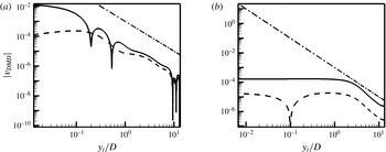
Point spectra of vertical velocity taken at locations inside the nozzle show the same dominant frequencies observed in the shear layer. Figure 23 shows the spectra in the symmetry plane at
 $(x/D,y/D)=(-0.49,-0.21)$
location and we see that the same frequencies are dominant for both
 $R=2$
and 4. Note that that the unsteadiness is higher for
 $R=2$
when compared to
 $R=4$
based on the amplitude of the spectra. To verify the nature of the disturbance inside the nozzle, we extract
 $v$
fluctuation magnitude of the dominant shear layer frequencies from DMD and plot it with distance from the jet exit in figure 24. Note that
 $y/D$
in the figure points away from the crossflow or into the nozzle. Based on the magnitude of the
 $v$
fluctuation from DMD, the dominant frequencies observed inside the nozzle appear to be due to the disturbances that originate from the shear layer oscillations. For both
 $R=2$
and 4, it can be observed that the disturbance is roughly constant until a certain location inside the nozzle beyond which it decays as
 $y^{-2}$
. It is interesting to note that the shear layer disturbances are dominant further inside the nozzle for
 $R=4$
as compared to
 $R=2$
.
Vertical velocity fluctuation magnitude from DMD variation along the nozzle centreline for
 $R=2$
(a) and
 $St=0.65$
(——) and 1.3 (– – –) and for
 $R=4$
(b) and
 $St=0.39$
(——) and 0.78 (– – –). An analytical decay corresponding to
 $v=y_{i}^{-2}$
(— ⋅ —) is also shown. Here,
 $y_{i}/D$
represents distance from the jet exit which increases as we move closer to the nozzle entrance.

6.2. Effect of simulating the nozzle for
 $R=2$

Past studies (Bagheri et al.
Reference Bagheri, Schlatter, Schmid and Henningson2009; Schlatter et al.
Reference Schlatter, Bagheri and Henningson2011; Ilak et al.
Reference Ilak, Schlatter, Bagheri and Henningson2012) have simulated the jet in crossflow problem by assuming a profile at the jet exit without solving for a nozzle or pipe. However, the influence of simulating the nozzle is not clear. Hence we simulate the
 $R=2$
flow without the nozzle (
 $R2_{nn}$
) but prescribe the mean flow from the
 $R2$
simulation to assess the effect of simulating the nozzle. From figure 11, it was observed that a separation vortex exists close to the jet exit due to the adverse pressure imposed by the crossflow fluid for
 $R=2$
. Also, figure 5 showed that the jet exit profile was more asymmetric for
 $R=2$
. Due to these two factors, it is expected that simulating the nozzle would have a greater effect for
 $R=2$
flow and hence we simulate this flow without the nozzle.


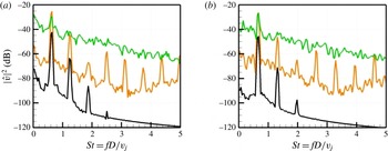
Figure 25 shows the
 $v$
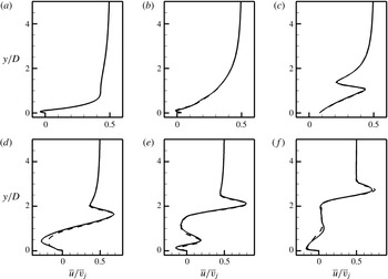
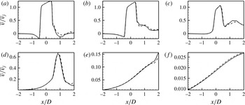
velocity spectra obtained at the same locations as in figure 4 with and without the nozzle. Note that good agreement is observed indicating that the shear layer instability is captured without the presence of the nozzle. Figure 26 compares the mean streamwise velocity variation along the wall normal direction for the simulations with and without the nozzle. The statistics reported were taken over 2 flow-through domain times for both flows. Overall, very good agreement is observed between the flows with and without the nozzle. Minor differences are observed at
 $x/D=0.5$
which could be due to the unsteadiness (although small in magnitude) at the trailing edge of the nozzle exit which is neglected in the simulation without the nozzle. Figure 27 shows the streamwise variation of the vertical velocity at various locations along the jet trajectory. Closest to the jet exit, minor differences can be observed between the profiles close to the trailing edge similar to those observed at
 $x/D=0.5$
in figure 26. Overall, again good agreement is observed between the simulations
 $R2$
and
 $R2_{nn}$
.
Since the difference between the simulations with and without the nozzle is small, it can be concluded that the role of the nozzle lies in setting up the mean flow at the jet exit which is then responsible for the shear layer instabilities. The mean jet exit velocity interacts with the crossflow boundary layer and undergoes a Kelvin–Helmholtz type instability resulting in the roll up of the upstream shear layer.
Wall normal variation of mean streamwise velocity with (——) and without (– – –) simulating the nozzle is shown for
 $R=2$
. Note that the curves agree well with each other indicating the minimal influence of simulating the nozzle for this flow. (a)
 $x/D=-1.0$
, (b)
 $x/D=-0.5$
, (c)
 $x/D=0.0$
, (d)
 $x/D=0.5$
, (e)
 $x/D=1.0$
, (f)
 $x/D=2.0$
.

Streamwise variation of mean wall normal velocity with (——) and without (– – –) simulating the nozzle is shown for
 $R=2$
. Note that the curves agree well with each other indicating the minimal influence of simulating the nozzle for this flow. (a)
 $y/D=0.25$
, (b)
 $y/D=0.5$
, (c)
 $y/D=1.0$
, (d)
 $y/D=2.0$
, (e)
 $y/D=3.0$
, (f)
 $y/D=5.0$
.

Mean vertical velocity variation with
 $x$
in the symmetry plane at the jet exit for
 $R2$
and
 $R2_{nn}$
(——),
 $R2_{p1}$
(– – –) and
 $R2_{m1}$
(— ⋅ —).

7. Effect of shear layer thickness
To assess the effect of increasing the shear layer thickness of the jet for
 $R=2$
, we perform simulations with a pipe-like velocity profile and velocity ratio of 2 based on the mean (
 $R2_{m1}$
) and peak velocities (
 $R2_{p1}$
). Note that the nozzle is not simulated for these flows. A symmetric profile is prescribed for the jet exit velocity similar to Bagheri et al. (Reference Bagheri, Schlatter, Schmid and Henningson2009) and Rowley et al. (Reference Rowley, Mezic, Bagheri, Schlatter and Henningson2009):
 $$\begin{eqnarray}\displaystyle v(r)=v_{j}(1-r^{2})\exp \left(-\left(\frac{r}{0.7}\right)^{4}\right), & & \displaystyle\end{eqnarray}$$
where
 $r$
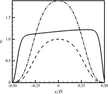
is non-dimensionalized by the maximum radius of the jet exit. Figure 28 shows the variation of mean vertical velocity of the jet in the symmetry plane at the jet exit. Here,
 $x/D$
is the streamwise direction of the crossflow boundary layer. Note that the velocity profile is axisymmetric for
 $R2_{p1}$
and
 $R2_{m1}$
flows which is not the case for
 $R2$
and
 $R2_{nn}$
. The maximum velocity at
 $r=0$
is
 $v_{j}$
which is 1 for
 $R2_{p1}$
and 1.889 for
 $R2_{m1}$
. Note that
 $v_{j}$
between
 $R2_{p1}$
and
 $R2_{m1}$
varies by nearly a factor of 2 and could account for some of the differences observed between the two flows. The maximum velocity at the jet exit (or centreline velocity) is used to define
 $St=fD/v_{j}$
.
Instantaneous isocontours of
 $Q$
coloured by streamwise velocity contours for
 $R2_{p1}$
(a) and
 $R2_{m1}$
(b) showing the vortical features.

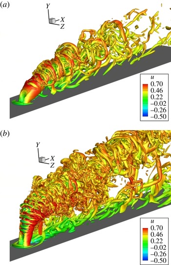
Figure 29 shows instantaneous vortical features of the flow using isocontours of the
 $Q$
criterion coloured by the streamwise velocity (
 $u$
) for
 $R2_{p1}$
and
 $R2_{m1}$
flows. Note that the flow features are very different from
 $R2$
flow in figure 9. The vortex rings for these flows appear coherent for long distances downstream of the jet which is not the case for
 $R2$
where the flows breaks down into smaller scales quickly. Also, for
 $R2_{p1}$
and
 $R2_{m1}$
, dominant vortical features are visible at the wall even at very large distances downstream of the jet. The jet bends more for
 $R2_{p1}$
as compared to
 $R2_{m1}$
due to a lower net momentum of the jet as compared to the crossflow. Also, for
 $R2$
, closer to the jet exit, vortical features correspond to the upstream shear layer roll up which is highest in the spanwise symmetry plane. On the other hand, for
 $R2_{p1}$
and
 $R2_{m1}$
flows, closer to the jet exit, it can be observed that the vortical activity is highest in the
 $x=0$
plane at the sides of the jet. The roll up of the shear layer also does not occur immediately at the jet exit which was the case for
 $R2$
.
Instantaneous spanwise vorticity contours in the symmetry plane (a,c,e) and mean
 $\overline{u^{\prime }u^{\prime }}$
contours in the
 $x=0$
plane (b,d,f) for
 $R2$
(a,b),
 $R2_{p1}$
(c,d) and
 $R2_{m1}$
(e,f) respectively.

Figure 30 shows the instantaneous spanwise vorticity contours (
 ${\it\omega}_{z}$
) in the spanwise symmetry plane and the
 $\overline{u^{\prime }u^{\prime }}$
in the
 $x=0$
plane (centre of the jet) for the
 $R2$
,
 $R2_{p1}$
and
 $R2_{m1}$
flows. While coherent roll up of the upstream shear layer is observed for
 $R2$
, the roll up of the upstream shear layer is delayed for
 $R2_{p1}$
and
 $R2_{m1}$
. For the
 $R2_{m1}$
flow, the trailing edge shear layer sheds before upstream shear layer. Thus, we see that the jet exit profile has a significant effect on the shear layer characteristics of the jet in crossflow. To assess the nature of the initial roll up of the shear layer, we compare the
 $\overline{u^{\prime }u^{\prime }}$
contours in the
 $x=0$
plane for the three flows. We see that for
 $R2$
, the unsteadiness is highest in the symmetry plane with the shape consistent with an unsteady shear layer roll up based on the location of the maximum (
 $y/D\approx 1.2$
) and the corresponding instantaneous
 ${\it\omega}_{z}$
contour. Interestingly, for the
 $R2_{p1}$
flow, we see that the unsteadiness is highest on either side of the symmetry plane which does not correspond to a shear layer roll up at this location. The shape of the unsteadiness resembles a boundary layer wake-type instability which appears to be dominant close to the jet exit. For the
 $R2_{m1}$
flow, the unsteadiness is again maximum at the symmetry plane and corresponds to the location at which the upstream shear layer begins to shed from the
 ${\it\omega}_{z}$
contours.
Note that the
 $R2_{m1}$
flow is similar to the experimental condition of Getsinger et al. (Reference Getsinger, Gevorkyan, Smith and Karagozian2014) for a jet issuing out of a pipe with
 $R=2.8$
and a jet
 $Re_{j}=1900$
. However, the two flows are different based on the spanwise vorticity contours in the current simulations and the acetone passive scalar visualization of Getsinger et al. (Reference Getsinger, Gevorkyan, Smith and Karagozian2014). This could be due to the asymmetry in the mean jet exit profile induced by the crossflow in the experiments which is not accounted for when imposing a steady symmetric profile in the current simulations. Muppidi & Mahesh (Reference Muppidi and Mahesh2005) have shown that the jet exit profile has a significant effect on the near field characteristics. The asymmetry in the jet exit profile affects the pressure gradient upstream of the jet which alters the stability characteristics of the counter-current mixing layer obtained in the upstream mixing layer. As discussed in § 5.4, the stability characteristics of the upstream mixing layer has a significant role in determining the nature of the jet shear layer.
Vertical and spanwise velocity spectra along the leading-edge shear layer are shown for
 $R2_{p1}$
(a) and
 $R2_{m1}$
(c). The spatial locations (
 $x/D,y/D$
) correspond to black line (
 $-0.5$
, 0.1), orange line (0.006, 0.854), green line (0.654, 1.614), blue line (1.432, 2.238), grey line (
 $-2.08$
, 0.137) and purple line (0.47, 1.03). Spectral energy variation with Strouhal number from DMD is also shown for
 $R2_{p1}$
(b) and
 $R2_{m1}$
(d).

DMD was performed for
 $R2_{p1}$
and
 $R2_{m1}$
flows to examine the dominant flow features and compare it to
 $R2$
. DMD was performed for the full three-dimensional velocity field with 200 snapshots at an interval of
 ${\rm\Delta}tD/\overline{v}=0.33$
and
 ${\rm\Delta}tD/v_{j}=0.33$
for
 $R2_{m1}$
and
 $R2_{p1}$
respectively. Note that the time interval between the snapshots is
 ${\rm\Delta}tD/u_{\infty }=0.66$
for
 $R2$
,
 $R2_{p1}$
and
 $R2_{m1}$
flows. Vertical and spanwise velocity spectra for
 $R2_{p1}$
and
 $R2_{m1}$
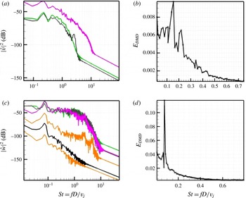
respectively taken along the leading-edge shear layer (at the same locations as figure 4) and the energy obtained from DMD are shown in figure 31. Note that
 $St=fD/v_{j}=0.22$
and
 $St=fD/v_{j}=0.075$
are dominant along the shear layer for
 $R2_{p1}$
and
 $R2_{m1}$
, respectively. The spanwise velocity spectra is shown for the
 $R2_{m1}$
flow since it shows the dominant frequency obtained from DMD. The same
 $St$
is obtained from both the DMD analysis and velocity spectra for
 $R2_{m1}$
. For
 $R2_{p1}$
, the most dominant mode from DMD is
 $St=0.15$
while another dominant mode is obtained at
 $St=0.22$
which corresponds to the
 $St$
obtained from velocity spectra in the upstream shear layer. Note that this
 $St$
is much lower than was observed for the
 $R2$
flow with the nozzle. However, note that the same
 $St$
is dominant along the shear layer indicating an absolute type instability as observed for
 $R2$
although the spectra looks more broadband when compared to
 $R2$
. Note that the
 $St$
observed for
 $R2_{p1}$
is similar to the
 $St=0.14$
observed by Rowley et al. (Reference Rowley, Mezic, Bagheri, Schlatter and Henningson2009) for
 $R=3$
and
 $Re=1650$
(based on peak jet velocity and diameter of the jet) for the simulation without the nozzle.
Isocontours of the
 $w$
velocity obtained from DMD of the most dominant mode corresponding to
 $St=0.65$
, 0.15 and 0.075 for
 $R2$
(a),
 $R2_{p1}$
(b) and
 $R2_{m1}$
(c) respectively. Red colour indicates a positive value while blue indicates a negative value.

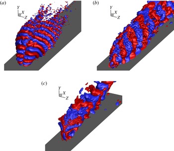
The spatial modes corresponding to the dominant frequencies seen from the DMD energy spectra are shown in figure 32 for
 $R2$
,
 $R2_{p1}$
and
 $R2_{m1}$
flows. Isocontours of the
 $w$
velocity obtained from DMD are shown. Positive isocontours are shown in red while negative isocontours are shown in blue. It can be seen that while the
 $R2$
flow is antisymmetric in
 $w$
,
 $R2_{p1}$
and
 $R2_{m1}$
flows are symmetric in
 $w$
. Note that modes that are antisymmetric in
 $w$
are symmetric in
 $u$
,
 $v$
and vice versa. Bagheri et al. (Reference Bagheri, Schlatter, Schmid and Henningson2009) observe both symmetric and antisymmetric modes from a global stability analysis of a jet in crossflow at
 $R=3$
at similar
 $Re$
and find that the shear layer symmetric modes are most unstable at
 $R=3$
. However, the dominant modes from
 $R2_{p1}$
and
 $R2_{m1}$
indicate that antisymmetric wake modes are more dominant possibly due to the lower momentum of the jet. Based on the nature of the dominant flow features and the dominant frequency, we see that the jet exit profile has a significant effect on the nature of the flow field and the shear layer characteristics. Thus, having a physically relevant jet exit profile is paramount to predict the shear layer characteristics of the complex jet in crossflow interactions at the values of
 $R$
studied in this paper.
8. Summary
Direct numerical simulation was performed of transverse jets for
 $R=2$
and 4 under the same conditions as the experiments of Megerian et al. (Reference Megerian, Davitian, Alves and Karagozian2007) to study the shear layer characteristics of the flow. The simulations capture the shear layer instability observed in the experiments and observe that the same frequency is dominant along the shear layer for
 $R=2$
flow, while different frequencies are dominant along the shear layer for
 $R=4$
. It was observed that the region of minimum pressure was downstream of the jet for
 $R=2$
while it was along the jet for
 $R=4$
. Also, strong oscillations in the spanwise velocity was observed for
 $R=2$
downstream of the jet while no such behaviour was observed for
 $R=4$
. DMD of the full three-dimensional flow field was performed and was able to reproduce the dominant frequencies obtained from shear layer velocity spectra. DMD showed that shear layer modes were dominant for both
 $R=2$
and 4 with a three-dimensional roll up of the shear layer. Also, the
 $St=0.78$
mode lies closer to the flat plate when compared to the
 $St=0.39$
mode for
 $R=4$
, consistent with different frequencies being dominant along the leading shear layer. A counter-current mixing layer-type region was observed in the upstream shear layer and the mixing layer ratio based on the minimum
 $v$
velocity upstream of the jet was
 ${\approx}\!1.44$
for
 $R=2$
flow and
 ${\approx}\!1.2$
for
 $R=4$
flow which is consistent with the critical value of 1.32 obtained by the experiments of Strykowski & Niccum (Reference Strykowski and Niccum1991) and 1.315 obtained by Huerre & Monkewitz (Reference Huerre and Monkewitz1985) for transition from absolute to convective instability. It was observed that the effect of simulating the nozzle for
 $R=2$
on the mean flow and shear layer characteristics was small when the jet exit velocity was prescribed with the mean flow obtained from the simulation with nozzle. Thus, the role of the nozzle was in setting up a mean flow at the jet exit which determines the stability characteristics of the flow. However, changing the jet exit velocity profile had a significant effect on both the nature of the flow field and the shear layer characteristics. A symmetric pipe-like profile was prescribed at the jet exit for simulations corresponding to a velocity ratio of 2 based on peak and mean jet exit velocity. It was observed that lower frequencies were dominant and the shear layer roll up was delayed as compared to the flow with nozzle. The dominant DMD modes were antisymmetric in nature as opposed to the symmetric modes observed for the flows with nozzle, further indicating that the nozzle has a significant effect on the instability characteristics of a jet in crossflow.
Acknowledgements
This work was supported by AFOSR grant FA9550-11-1-0128. Computer time for the simulations was provided by the Minnesota Supercomputing Institute (MSI) and Texas Advanced Computing Center through the XSEDE allocation. We thank Professor Karagozian for providing experimental data and S. Muppidi for useful discussions. We also thank E. Mussoni for performing preliminary simulations.