



1. Introduction
The configuration in which a slow liquid stream is destabilized by a fast gas stream is both a classical fluid mechanics problem and a configuration encountered in many applications related to combustion (Lefebvre Reference Lefebvre1989). Injecting kerosene and air this way in turbo-reactors leads, for example, to the formation of a very efficient spray, i.e. one whose droplets are very small. This configuration has therefore been the object of many studies, but in spite of the attention it has garnered its mechanism is still a matter of controversy. Is it an inviscid or a viscous instability? This is the question we wish to address in the present paper.
Raynal (Reference Raynal1997) and Raynal et al. (Reference Raynal, Villermaux, Lasheras and Hopfinger1997) carried out a series of experiments on this simple two-phase flow configuration: a slow liquid stream (velocity
 $U_{L}$
, width 10 cm, height
 $H_{L}=1~\text{cm}$
) flowing on a solid plate is destabilized by a fast gas stream (velocity
 $U_{G}$
, width 10 cm, height
 $H_{G}=1~\text{cm}$
). Long-wavelength waves form, and are rapidly convected away from injection and subsequently atomized into droplets. These waves have a ‘long’ wavelength in the sense that it is large compared to other lengths in the problem: the thicknesses of the gas and liquid streams, and especially the gas and liquid vorticity thicknesses,
 ${\it\delta}_{G}$
and
 ${\it\delta}_{L}$
. Wave frequency was measured, and experimental results confronted to a simple inviscid stability analysis generalizing that of Rayleigh (Reference Rayleigh1879). Experimental trends, and a good order of magnitude of the frequency, can be captured with this approach (Raynal Reference Raynal1997; Raynal et al.
Reference Raynal, Villermaux, Lasheras and Hopfinger1997). The mechanism driving the instability is then similar to the classical Kelvin–Helmholtz one, but wavelength selection occurs through the size of the gas vorticity thickness
 ${\it\delta}_{G}$
. The scaling obtained for the most unstable frequency can be recovered from a simple energy budget for the velocity perturbation
 $u$
, by writing that the perturbation is fed by the Reynolds stress in the gas phase:
 $$\begin{eqnarray}\frac{\text{d}{\it\rho}_{L}u^{2}}{\text{d}t}=\frac{{\it\rho}_{G}u^{2}U_{G}}{{\it\delta}_{G}}\quad \Rightarrow \quad {\it\omega}\sim \frac{{\it\rho}_{G}}{{\it\rho}_{L}}\frac{U_{G}}{{\it\delta}_{G}},\end{eqnarray}$$
where
 ${\it\rho}_{G}$
and
 ${\it\rho}_{L}$
are the gas and liquid densities and
 $U_{G}$
the base flow gas velocity. This scaling law is in good agreement with experiments (Raynal Reference Raynal1997; Raynal et al.
Reference Raynal, Villermaux, Lasheras and Hopfinger1997). The velocity associated with these waves can be predicted by a similarly simple phenomenological argument. It is the velocity of the frame in which dynamic pressure in the liquid is balanced by dynamic pressure in the gas (Dimotakis Reference Dimotakis1986), namely,
 $$\begin{eqnarray}U_{c}=\frac{\sqrt{{\it\rho}_{L}}U_{L}+\sqrt{{\it\rho}_{G}}U_{G}}{\sqrt{{\it\rho}_{G}}+\sqrt{{\it\rho}_{L}}}.\end{eqnarray}$$
Measurements indicate that the experimentally measured velocity is quite close to the velocity given by (1.2) (Raynal Reference Raynal1997). In the limit of large gas velocities, these simple scaling laws imply in particular that the wavelength will be given by (Eggers & Villermaux Reference Eggers and Villermaux2008)
 $$\begin{eqnarray}{\it\lambda}\sim \sqrt{{\it\rho}_{L}/{\it\rho}_{G}}\,{\it\delta}_{G}.\end{eqnarray}$$
A similar configuration has been studied by Marmottant & Villermaux (Reference Marmottant and Villermaux2004), for a different geometry: a round liquid jet destabilized by an annular parallel gas stream. This study evidences the same scaling laws seen in the planar case for the frequency and wavelength of the axial wavy perturbations.
Though they capture the correct scaling laws, the values predicted by the inviscid approach underpredict wave frequency. Seeking to improve the prediction of the inviscid stability analysis, Matas, Marty & Cartellier (Reference Matas, Marty and Cartellier2011) extended it to velocity profiles mimicking the velocity deficit observed just downstream of the injection, where liquid velocity close to the interface is observed to be much smaller than in the liquid bulk. This modified analysis increases predicted frequencies by about 50 %, and therefore offers a relatively good frequency prediction. However, Matas et al. (Reference Matas, Marty and Cartellier2011) observed that the inviscid analysis strongly underpredicts spatial growth rates, and fails to capture the steep increase of growth rate with gas velocity.
In order to clarify the issue of the nature of the instability and of the potential effect of viscosity, Boeck & Zaleski (Reference Boeck and Zaleski2005) carried out a temporal linear stability analysis including viscosity. They found that, when viscosity is included in the temporal stability analysis, the most unstable mode for the conditions of the experiments of Marmottant & Villermaux (Reference Marmottant and Villermaux2004) is actually a purely viscous mode. This mode is akin to the mode evidenced by Yih (Reference Yih1967), and discussed by Hooper & Boyd (Reference Hooper and Boyd1983, Reference Hooper and Boyd1987) and Charru & Hinch (Reference Charru and Hinch2000), whose mechanism in the limit of short wavelengths has been discussed by Hinch (Reference Hinch1984): it is triggered by the jump in viscosity, and therefore in shear rate, across the interface. The order of magnitude of the growth rate associated with this viscous mode is consistent with experiments, but predicted frequencies largely overestimate experimental ones. The paradox that a simplified inviscid analysis performs better than a viscous one has been partially solved by Fuster et al. (Reference Fuster, Matas, Marty, Popinet, Hoepffner, Cartellier and Zaleski2013) and Otto, Rossi & Boeck (Reference Otto, Rossi and Boeck2013): by carrying out a spatiotemporal analysis including viscosity, they showed that an absolute instability may be predicted for some of the experimental conditions of Matas et al. (Reference Matas, Marty and Cartellier2011), and that, when this absolute instability occurs, there is a relatively good agreement between experiments on the planar geometry and predictions. The mechanism is in this case purely viscous. However, when the instability is predicted to be convective (for most of the experimental conditions of Matas et al. (Reference Matas, Marty and Cartellier2011)), frequency remains strongly overpredicted. As for growth rates, Otto et al. (Reference Otto, Rossi and Boeck2013) noticed that the theoretical growth rates associated with the experimentally observed frequency are in agreement with experimental ones: in other words, if another frequency selection mechanism were able to provide the experimental frequency, then frequency and growth rate would agree with experiments. Comparison with the experimental data of Marmottant & Villermaux (Reference Marmottant and Villermaux2004) shows a relatively good agreement, even when the instability is convective.
There are therefore two questions we want to address in this paper:
-
(a) Most of the experimental data of Matas et al. (Reference Matas, Marty and Cartellier2011) remain overpredicted by the spatiotemporal viscous approach of Otto et al. (Reference Otto, Rossi and Boeck2013), and this points to a still missing ingredient in the viscous spatiotemporal theory.
-
(b) The initial inviscid approach of Raynal (Reference Raynal1997) and Marmottant & Villermaux (Reference Marmottant and Villermaux2004) seemed to capture very well experimental scaling laws. However, it is predicted by Otto et al. (Reference Otto, Rossi and Boeck2013) via an energy budget that the most unstable mode for the conditions of these experiments is dominated by the viscous mechanism studied by Yih (Reference Yih1967) and others. Why therefore is the simple inviscid approach so successful?
In the experiment, the liquid and gas streams are confined within lengths smaller than the observed longitudinal wavelength. The fact that confinement can trigger absolute instability in shear flows has been evidenced in recent years by Healey (Reference Healey2007, Reference Healey2009), Juniper (Reference Juniper2008) and Rees & Juniper (Reference Rees and Juniper2010). The absolute instability observed by Fuster et al. (Reference Fuster, Matas, Marty, Popinet, Hoepffner, Cartellier and Zaleski2013) and Otto et al. (Reference Otto, Rossi and Boeck2013) is of a different type, occurring between the shear instability branch and a branch located below, and is controlled by surface tension. We investigate in the following how including in the spatiotemporal analysis a confinement similar to the experimental one affects predictions.
2. Method
We consider Navier–Stokes equations for a base flow
 $\boldsymbol{U}=(U(y),0,0)$
and a small perturbation
 $\boldsymbol{u}(x,y,t)$
(coordinate system shown in figure 1). After linearization of this two-dimensional problem, we look for normal mode solutions of the form
 $\tilde{\boldsymbol{u}}(k,y,{\it\omega})\text{e}^{\text{i}(kx-{\it\omega}t)}$
and obtain the classical Orr–Sommerfeld equation for the cross-stream velocity component of the perturbation in Fourier space
 $\tilde{v}(k,y,{\it\omega})$
in each fluid (Otto et al.
Reference Otto, Rossi and Boeck2013). Boundary conditions are a solid wall at
 $y=-H_{L}$
, and another solid wall at a distance
 $y=L_{G}$
on the gas side. For the present study, we take
 $L_{G}$
to be 10 times larger than other scales in the problem, typically
 $L_{G}=30\max (H_{G},H_{L})$
, to ensure that no confinement occurs due to this wall. The method we use for solving this problem is different from the method used by Fuster et al. (Reference Fuster, Matas, Marty, Popinet, Hoepffner, Cartellier and Zaleski2013) or Otto et al. (Reference Otto, Rossi and Boeck2013): instead of using a spectral method, we solve for the velocity perturbation
 $\tilde{v}(k,y,{\it\omega})$
in real space, with a Runge–Kutta method. In each phase, integration is carried out from the solid wall, where both velocity components must be zero, to the interface, where continuity of tangential and normal velocities, as well as continuity of tangential and normal stresses, is enforced. Surface tension and gravity normal to the interface, which may affect prediction for large wavelength, are included in the normal stress equation. In order to ensure that both solutions satisfying
 $\tilde{v}=0$
and
 $\partial \tilde{v}/\partial y=0$
at the solid walls remain independent during integration, we orthonormalize the associated four-dimensional vectors at each time step within the Runge–Kutta algorithm with the procedure described in Asmolov (Reference Asmolov1999) and Matas, Morris & Guazzelli (Reference Matas, Morris and Guazzelli2009). The dispersion relation is then solved with a shooting method (two-dimensional Newton–Raphson method). Contrary to the spectral method, the present shooting method does not provide us with the whole set of eigenmodes: however, it is well adapted to the present aim, which is to focus on a given set of parameters close to experimental conditions.
Sketch showing the typical base flow profile, including finite liquid and gas stream thicknesses.

We chose the same family of base flow profiles used by Otto et al. (Reference Otto, Rossi and Boeck2013), namely a sum of error functions accounting for the wake due to the splitter plate between the liquid and gas streams. Additional error function cutoff terms are added to account for the finite
 $H_{G}$
and
 $H_{L}$
that we wish to include in the present study:
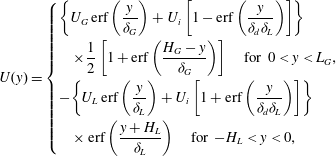 $$\begin{eqnarray}U(y)=\left\{\begin{array}{@{}l@{}}\displaystyle \left\{U_{G}\,\text{erf}\left(\frac{y}{{\it\delta}_{G}}\right)+U_{i}\left[1-\text{erf}\left(\frac{y}{{\it\delta}_{d}{\it\delta}_{L}}\right)\right]\right\}\\ \quad \displaystyle \times \frac{1}{2}\left[1+\text{erf}\left(\frac{H_{G}-y}{{\it\delta}_{G}}\right)\right]\quad \text{for }0<y<L_{G},\\ \displaystyle -\!\left\{U_{L}\,\text{erf}\left(\frac{y}{{\it\delta}_{L}}\right)+U_{i}\left[1+\text{erf}\left(\frac{y}{{\it\delta}_{d}{\it\delta}_{L}}\right)\right]\right\}\\ \quad \displaystyle \times \,\text{erf}\left(\frac{y+H_{L}}{{\it\delta}_{L}}\right)\quad \text{for }-H_{L}<y<0,\end{array}\right.\end{eqnarray}$$
where
 $U_{i}$
is the interface velocity
 $U_{i}=(U_{G}{\it\mu}_{G}/{\it\delta}_{G}+U_{L}{\it\mu}_{L}/{\it\delta}_{L})/({\it\mu}_{G}+{\it\mu}_{L}){\it\delta}_{d}{\it\delta}_{L}$
, with
 ${\it\mu}_{G}$
and
 ${\it\mu}_{L}$
the dynamical viscosities of gas and liquid, and
 ${\it\delta}_{L}$
the liquid boundary layer. The dimensionless parameter
 ${\it\delta}_{d}$
allows control of the amplitude of the velocity deficit: for
 ${\it\delta}_{d}=1$
there is no velocity deficit (as in figure 1), while for
 ${\it\delta}_{d}\ll 1$
the interface velocity goes down to zero (Otto et al.
Reference Otto, Rossi and Boeck2013).
In order to facilitate comparison with experiments, we set the gas vorticity thickness to the value measured in experiments. The experimental
 ${\it\delta}_{G}$
is well approximated (see Raynal Reference Raynal1997; Matas et al.
Reference Matas, Marty and Cartellier2011) by
 ${\it\delta}_{G}=6H_{G}/\sqrt{U_{G}H_{G}{\it\rho}_{G}/{\it\mu}_{G}}$
. The liquid boundary layer is set to a constant value of
 ${\it\delta}_{L}=500~{\rm\mu}\text{m}$
, close to the value measured in the experiment for the relevant range of liquid velocities (particle image velocimetry measurement). Note finally that the above expression is a fit of the mean velocity profile: though experimental air and water flows are turbulent for the Reynolds numbers of interest, fluctuations are not included in the present analysis.
3. Results and discussion
We now confront the predictions obtained with this method to the air–water experimental data of Matas et al. (Reference Matas, Marty and Cartellier2011). We first consider their series of data obtained at a fixed
 $U_{G}=27~\text{m}~\text{s}^{-1}$
: the prediction of the viscous spatiotemporal analysis without confinement for this series overestimates the experimental data by a factor of 2 for most liquid velocities (see figure 31d of Otto et al.
Reference Otto, Rossi and Boeck2013). Figure 2 shows what happens for
 $U_{L}=0.26~\text{m}~\text{s}^{-1}$
when a confinement similar to the experimental one is taken into account and when
 ${\it\omega}_{i}$
, the imaginary part of
 ${\it\omega}$
, is reduced: a confinement branch appears along the
 $k_{i}$
axis, and pinching between this branch and the shear instability branch occurs for positive
 ${\it\omega}_{0i}$
. While the shear instability branch involved in the pinching observed by Otto et al. (Reference Otto, Rossi and Boeck2013) at large
 $U_{L}$
is what they call the weaker mode (as in figure 25b of their paper), the branch involved in the pinching mechanism of figure 2 is the stronger mode, which extends to lower wavenumbers. The confinement branch involved in the pinching is of the type described in Healey (Reference Healey2007): it arises because of the oscillatory nature of the confined perturbation when
 $k$
is close to the imaginary axis. The frequency predicted without taking confinement into account would be the frequency corresponding to the minimum of the negative growth rate (there is no pinch point on the weaker mode for the conditions of figure 2), namely 66 Hz, while the pinching caused by confinement occurs for a much lower frequency of 28 Hz. The latter frequency is much closer to the experimental frequency
 $f_{exp}=28.8~\text{Hz}$
.
Pinching at positive
 ${\it\omega}_{0i}$
occurs between confinement and shear controlled branches when confinement is taken into account;
 $U_{G}=27~\text{m}~\text{s}^{-1}$
,
 $U_{L}=0.26~\text{m}~\text{s}^{-1}$
,
 ${\it\delta}_{d}=1$
,
 $H_{G}=1~\text{cm}$
and
 $H_{L}=1~\text{cm}$
. Symbols correspond to
 ${\it\omega}_{r}$
in the range
 $(80{-}680)~\text{s}^{-1}$
.

For the case of an absolute instability, nonlinearity is expected to affect the properties of the eigenmode at the pinch point, and comparison between growth rate at the pinch point and experimental spatial growth rate is therefore not attempted. It is however interesting to note the value of the wavenumber at the pinch point: figure 2 shows that the pinching induces a major reduction in the predicted wavenumber, from
 $k_{r}\approx 720~\text{m}^{-1}$
down to
 $k_{r}\approx 140~\text{m}^{-1}$
. The corresponding phase velocity
 ${\it\omega}_{r}/k_{r}$
(we denote
 ${\it\omega}_{r}$
the real part of
 ${\it\omega}$
) is then about
 $1.28~\text{m}~\text{s}^{-1}$
, very close to the value given by (1.2),
 $U_{c}=1.2~\text{m}~\text{s}^{-1}$
. Wave velocity was not measured in the experiment of Matas et al. (Reference Matas, Marty and Cartellier2011), but previous experiments by Raynal (Reference Raynal1997) and Ben Rayana (Reference Ben Rayana2007) had both found wave velocity in close agreement with
 $U_{c}$
. In addition, expression (1.2) for velocity
 $U_{c}$
was derived by Dimotakis (Reference Dimotakis1986) through a balance of dynamic pressure, and a similar expression was found by Matas et al. (Reference Matas, Marty and Cartellier2011) in the frame of the inviscid linear theory via an asymptotic expansion in the limit of low density ratio. This expression therefore corresponds to a perturbation driven by an inviscid mechanism: the fact that the predicted phase velocity is close to (1.2) is a first indication that the dominant mechanism for these
 ${\it\omega}$
and
 $k$
is inviscid. Note that the velocity associated with the most unstable modes in Fuster et al. (Reference Fuster, Matas, Marty, Popinet, Hoepffner, Cartellier and Zaleski2013) or Otto et al. (Reference Otto, Rossi and Boeck2013), which are viscous modes, is closer to
 $U_{i}$
and significantly lower than this estimate.
Figure 3 next shows how the predicted frequency compares to the experimental one (filled squares) for the experimental data at
 $U_{G}=27~\text{m}~\text{s}^{-1}$
for each of the six liquid velocities investigated. The asterisks show the prediction of Otto et al. (Reference Otto, Rossi and Boeck2013) for
 ${\it\delta}_{d}=0.1$
, a prediction that works well for the two higher velocities, but clearly fails for the four lower velocities. For
 ${\it\delta}_{d}=1$
the predictions of Otto et al. (Reference Otto, Rossi and Boeck2013) for all
 $U_{L}$
far exceed experimental data (see figure 31d of their paper), and are not shown here. The circles show the frequency obtained at pinching when confinement is taken into account, for
 ${\it\delta}_{d}=1$
(no velocity deficit): this frequency is in relatively good agreement with experimental data. Note that for the four lower liquid velocities the mode predicted by Otto et al. (Reference Otto, Rossi and Boeck2013) when
 ${\it\delta}_{d}=1$
is associated with a convective mode, and the present absolute instability caused by confinement is therefore expected to dominate. For
 ${\it\delta}_{d}=1$
and the two largest liquid velocities in this series, however, the pinching occurs at negative
 ${\it\omega}_{0i}$
, and the confinement mechanism is consequently not relevant.
Comparison at
 $U_{G}=27~\text{m}~\text{s}^{-1}$
between experimental data of Matas et al. (Reference Matas, Marty and Cartellier2011) (▪) and available spatiotemporal predictions: *, prediction by Otto et al. (Reference Otto, Rossi and Boeck2013), for
 ${\it\delta}_{d}=0.1$
; ○, prediction taking into account confinement without any velocity deficit (
 ${\it\delta}_{d}=1$
); ▫, prediction with confinement and a velocity deficit (
 ${\it\delta}_{d}=0.5$
).

If a velocity deficit is included in the base flow profile, the absolute instability is enhanced (i.e. it occurs at even larger
 ${\it\omega}_{0i}$
), and the frequency slightly increases too; these data are shown by the open squares in figure 3, for
 ${\it\delta}_{d}=0.5$
. If a stronger deficit is included (
 ${\it\delta}_{d}<0.4$
), the shear instability branch is displaced and the pinch point due to confinement disappears. Figure 4 shows the same comparison for the series of experimental data of Matas et al. (Reference Matas, Marty and Cartellier2011) at
 $U_{G}=22~\text{m}~\text{s}^{-1}$
, and the same agreement is found when confinement is included. Figure 5 shows the variation of the absolute growth rate
 ${\it\omega}_{0i}$
at the pinch point: it decreases when
 $U_{L}$
is increased, and eventually becomes negative for
 $U_{L}>0.6~\text{m}~\text{s}^{-1}$
. The inclusion of a moderate velocity deficit (
 ${\it\delta}_{d}=0.5$
, open squares) leads to a slight increase of
 ${\it\omega}_{0i}$
.
Comparison at
 $U_{G}=22~\text{m}~\text{s}^{-1}$
between experimental data of Matas et al. (Reference Matas, Marty and Cartellier2011) (▪) and available spatiotemporal predictions: *, prediction by Otto et al. (Reference Otto, Rossi and Boeck2013), for
 ${\it\delta}_{d}=0.1$
; ○, prediction taking into account confinement without any velocity deficit (
 ${\it\delta}_{d}=1$
).

Variation of the absolute growth rate
 ${\it\omega}_{0i}$
at the pinch point caused by the confinement branch, as a function of liquid velocity, for fixed
 $U_{G}=27~\text{m}~\text{s}^{-1}$
,
 $H_{G}=1~\text{cm}$
and
 $H_{L}=1~\text{cm}$
: ●,
 ${\it\delta}_{d}=1$
; ▫,
 ${\it\delta}_{d}=0.5$
. The growth rate decreases when liquid velocity is increased, and increases when a velocity deficit is included.

The fact that agreement between prediction and experiments occurs for
 ${\it\delta}_{d}=1$
at lower
 $U_{L}$
, while it occurs for smaller
 ${\it\delta}_{d}$
at larger
 $U_{L}$
, is consistent with the idea that the velocity deficit will be resorbed over a longer distance when the liquid velocity is larger. At any rate, only a global approach, in the sense introduced by Huerre & Monkewitz (Reference Huerre and Monkewitz1990), may clarify how mode selection occurs in the presence of strong spatial variations, when unstable modes predicted close to the splitter plate (where
 ${\it\delta}_{d}\ll 1$
) differ from those farther downstream (where
 ${\it\delta}_{d}=1$
).
In order to clarify the nature of the dominant mechanism for the new pinch point caused by confinement, we carry out an energy budget similar to the one introduced by Boomkamp & Miesen (Reference Boomkamp and Miesen1996) for temporal modes. The energy budget can be written as
 $$\begin{eqnarray}\frac{\text{d}E_{kin}}{\text{d}t}=\mathit{REY}_{L}+\mathit{REY}_{G}+\mathit{TAN}+\mathit{NOR}+\mathit{DIS}_{L}+\mathit{DIS}_{G}.\end{eqnarray}$$
Here
 $E_{kin}$
is the total kinetic energy of the eigenmode
 $(\text{gas}+\text{liquid})$
;
 $\mathit{REY}_{L}$
(respectively
 $\mathit{REY}_{G}$
) is the transfer of energy from the base flow to the perturbation via Reynolds stresses in the liquid (respectively gas) stream;
 $\mathit{TAN}$
is the work of tangential stresses;
 $\mathit{NOR}$
is the contribution of normal stresses (surface tension and gravity in the present case); and
 $\mathit{DIS}_{L}$
(respectively
 $\mathit{DIS}_{G}$
) is the dissipation in the liquid phase (respectively gas phase). The analytical expressions for each of these terms are very similar to the expressions given in Otto et al. (Reference Otto, Rossi and Boeck2013), and are not repeated here. The only differences here are that the wavenumber is complex, and that the kinetic energy variation term must be generalized to include a contribution from the spatial growth:
 $$\begin{eqnarray}\displaystyle \frac{\text{d}E_{kin}}{\text{d}t} & = & \displaystyle {\it\omega}_{i}\int _{-H_{L}}^{0}{\it\rho}_{L}(u^{2}+v^{2})\text{d}y-k_{i}\int _{-H_{L}}^{0}{\it\rho}_{L}(u^{2}+v^{2})U(y)\text{d}y\nonumber\\ \displaystyle & & \displaystyle +\,{\it\omega}_{i}\int _{0}^{L_{G}}{\it\rho}_{G}(u^{2}+v^{2})\text{d}y-k_{i}\int _{0}^{L_{G}}{\it\rho}_{G}(u^{2}+v^{2})U(y)\text{d}y.\end{eqnarray}$$
We compute the energy budget for the six data points of figure 3 showing the best agreement with experimental results, more precisely the four data points obtained with confinement for lower
 $U_{L}$
and
 ${\it\delta}_{d}=1$
(no velocity deficit), and the two points obtained by Otto et al. (Reference Otto, Rossi and Boeck2013) for
 $U_{L}=0.74$
and
 $1~\text{m}~\text{s}^{-1}$
(with a velocity deficit,
 ${\it\delta}_{d}=0.1$
). The energy contributions are normalized by the total positive kinetic energy rate. We omit the contribution of NOR, which is negligible for most of the present points. Table 1 shows that, for the four conditions for which confinement triggers the absolute instability, the mechanism is inviscid, and that the perturbation draws its energy from the gas side. This is consistent with phase velocity being close to
 $U_{c}$
(1.2). For the two data points at larger velocity, the mechanism is confirmed to be viscous, driven by the work of interfacial tangential stresses (Otto et al.
Reference Otto, Rossi and Boeck2013). Dissipation occurs almost exclusively in the gas phase.
Energy budget for the data (○) and (*) of figure 3. Values are as a percentage of the total (positive) kinetic energy rate.

The idea behind the generalized budget of (3.1) is to identify among the right-hand contributions which are dominant and which are negligible when at the pinch point. It might be tempting to carry out the energy budget in a more classical form, in order to avoid the generalization to spatiotemporal modes. However, for a purely temporal mode, the results would depend very much on how the
 $\{\text{spatiotemporal}\rightarrow \text{temporal}\}$
transposition is made. For a purely temporal mode at the same
 ${\it\omega}_{r}$
as the pinch point, for example, and conditions of the first line of table 1, the wavenumber would become
 $k_{r}\approx 380~\text{m}^{-1}$
instead of
 $k_{r}\approx 170~\text{m}^{-1}$
for the spatiotemporal mode. For these conditions, the energy budget says the temporal mode is 85 % viscous (the same budget would be found for the spatiotemporal mode at this larger
 $k_{r}$
). If a
 $\{\text{spatiotemporal}\rightarrow \text{spatial}\}$
comparison is carried out for the wavenumber of the pinch point, then the energy budget says the mode is 60 % viscous and 40 % viscous. Hence a transposition would be extremely sensitive to which
 ${\it\omega}$
and
 $k$
values are retained.
At any rate, the inviscid nature of the instability for the pinch point due to confinement is confirmed by figure 6, which shows the impact of a reduction of viscosity on spatial branches for the case
 $U_{G}=27~\text{m}~\text{s}^{-1}$
and
 $U_{L}=0.26~\text{m}~\text{s}^{-1}$
(conditions of figure 2). When viscosity is reduced, the shear branch is impacted, but the confinement branch is unchanged, and the pinch point remains at the same location. Frequency at the pinch point slightly decreases when viscosity is reduced, from
 $f=28~\text{Hz}$
for
 ${\it\nu}_{G}=1.5\times 10^{-5}~\text{m}~\text{s}^{-1}$
and
 ${\it\nu}_{L}=10^{-6}~\text{m}~\text{s}^{-1}$
down to
 $f=20~\text{Hz}$
for
 ${\it\nu}_{G}=1.5\times 10^{-7}~\text{m}~\text{s}^{-1}$
and
 ${\it\nu}_{L}=10^{-8}~\text{m}~\text{s}^{-1}$
.
Impact of a variation in viscosity on spatial branches for
 $U_{G}=27~\text{m}~\text{s}^{-1}$
,
 $U_{L}=0.26~\text{m}~\text{s}^{-1}$
and
 ${\it\delta}_{d}=1$
: *,
 ${\it\nu}_{G}=1.5\times 10^{-5}~\text{m}~\text{s}^{-1}$
,
 ${\it\nu}_{L}=10^{-6}~\text{m}~\text{s}^{-1}$
and
 ${\it\omega}_{i}=85~\text{s}^{-1}$
; ▫,
 ${\it\nu}_{G}=1.5\times 10^{-6}~\text{m}~\text{s}^{-1}$
,
 ${\it\nu}_{L}=10^{-7}~\text{m}~\text{s}^{-1}$
and
 ${\it\omega}_{i}=65~\text{s}^{-1}$
; ●,
 ${\it\nu}_{G}=1.5\times 10^{-7}~\text{m}~\text{s}^{-1}$
,
 ${\it\nu}_{L}=10^{-8}~\text{m}~\text{s}^{-1}$
and
 ${\it\omega}_{i}=50~\text{s}^{-1}$
;
 $+$
,
 ${\it\nu}_{G}=1.5\times 10^{-7}~\text{m}~\text{s}^{-1}$
,
 ${\it\nu}_{L}=10^{-6}~\text{m}~\text{s}^{-1}$
and
 ${\it\omega}_{i}=45~\text{s}^{-1}$
. The shear branch is displaced when viscosity is reduced, but the location of the pinch point associated with confinement remains unchanged.

This result is satisfying, because it explains the paradox exposed in the introduction, namely why the simplified analysis proposed by Raynal (Reference Raynal1997) was successful, and why the inclusion of viscosity in the analysis had degraded the quality of the prediction. The inclusion of viscosity gives rise to a much stronger shear mode based on the viscous mechanism (Boeck & Zaleski Reference Boeck and Zaleski2005; Otto et al. Reference Otto, Rossi and Boeck2013), but resonance due to confinement triggers an absolute instability for the lower-wavenumber part of the shear branch, which is dominated by the inviscid mechanism. This occurs for all the lower liquid velocity points of Matas et al. (Reference Matas, Marty and Cartellier2011), as in figure 3. For the larger liquid velocity conditions, we find that the shear branch is displaced away from the confinement branch, and the mechanism is then the one predicted by Otto et al. (Reference Otto, Rossi and Boeck2013), an absolute instability between the shear branch controlled by viscosity and a lower branch controlled by surface tension.
Change in the confinement branches when
 $H_{G}$
and
 $H_{L}$
are reduced, for fixed
 $U_{G}=27~\text{m}~\text{s}^{-1}$
,
 $U_{L}=0.26~\text{m}~\text{s}^{-1}$
,
 ${\it\delta}_{d}=1$
,
 ${\it\omega}_{i}=120~\text{s}^{-1}$
and
 ${\it\omega}_{r}$
in the range
 $(60{-}430)~\text{s}^{-1}$
: ●,
 $H_{G}=H_{L}=2~\text{cm}$
;
 $\times$
,
 $H_{G}=H_{L}=1~\text{cm}$
; ○,
 $H_{G}=H_{L}=0.5~\text{cm}$
.

Pinching for
 $U_{G}=27~\text{m}~\text{s}^{-1}$
,
 $U_{L}=0.26~\text{m}~\text{s}^{-1}$
,
 ${\it\delta}_{d}=1$
,
 ${\it\omega}_{i}=60~\text{s}^{-1}$
and
 ${\it\omega}_{r}$
in the range
 $(60{-}280)~\text{s}^{-1}$
: ○,
 $H_{G}=3~\text{cm}$
and
 $H_{L}=1~\text{cm}$
; *,
 $H_{G}=1~\text{cm}$
and
 $H_{L}=3~\text{cm}$
. Both thicknesses play a symmetric role.

The velocity profile considered in figure 1 includes both a finite
 $H_{G}$
and a finite
 $H_{L}$
. In order to clarify the influence of these thicknesses, we keep them equal and vary them, while keeping
 ${\it\delta}_{G}$
and
 ${\it\delta}_{L}$
constant and equal to their values for
 $H_{G}=H_{L}=H=1~\text{cm}$
. Figure 7 shows that the location of the confinement branch along the
 $k_{i}$
axis behaves as
 $1/H$
, and that the extension of the branches increases strongly with
 $1/H$
: these branches therefore set the order of magnitude of
 $k$
at the pinch point. If these thicknesses are distinct, we observe that their role is symmetric. Figure 8 shows two sets of branches obtained for (
 $H_{G}=3~\text{cm}$
;
 $H_{L}=1~\text{cm}$
) and for (
 $H_{G}=1~\text{cm}$
;
 $H_{L}=3~\text{cm}$
). Though experimentally a thick liquid and a thin gas stream may look quite different from a thin liquid stream and a thick gas stream, we find that the branches obtained in both situations are very close. They extend to the same
 $\mathit{real}(k)$
as the branch obtained for
 $H_{G}=H_{L}=1~\text{cm}$
, the smaller length, the only difference being that the absolute growth rate
 ${\it\omega}_{0i}$
is significantly smaller for
 $H_{G}\neq H_{L}$
than for
 $H_{G}=H_{L}$
. The fact that a symmetric confinement can enhance the absolute instability of a shear layer has already been pointed out in Healey (Reference Healey2009).
As shown in figure 3, the present mechanism dominates for the largest
 $U_{G}/U_{L}$
cases but is absent for the largest liquid velocities investigated. Figure 9 sheds light on this behaviour. When
 $U_{L}$
is increased, the maximum growth rate of the shear branch decreases. If the maximum growth rate of this branch, which is controlled by the viscous mechanism (Otto et al.
Reference Otto, Rossi and Boeck2013), is shifted above the location of the confinement branch, then the two branches cannot collide any more when
 ${\it\omega}_{i}$
is reduced.
Influence of liquid velocity
 $U_{L}$
, for fixed
 $U_{G}=27~\text{m}~\text{s}^{-1}$
,
 $H_{G}=H_{L}=1~\text{cm}$
,
 ${\it\delta}_{d}=1$
and
 ${\it\omega}_{i}=120~\text{s}^{-1}$
: ●,
 $U_{L}=0.26~\text{m}~\text{s}^{-1}$
; ○,
 $U_{L}=0.5~\text{m}~\text{s}^{-1}$
; *,
 $U_{L}=1~\text{m}~\text{s}^{-1}$
. The ranges of
 ${\it\omega}_{r}$
are respectively (120–370), (170–500) and
 $(260{-}820)~\text{s}^{-1}$
. When liquid velocity is increased, the shear branch is shifted away from the confinement branch.

Influence of vorticity thickness
 ${\it\delta}_{G}$
on
 ${\it\omega}_{r}$
(circles) and
 ${\it\omega}_{0i}$
(squares), for fixed
 $U_{G}=27~\text{m}~\text{s}^{-1}$
,
 $U_{G}=0.26~\text{m}~\text{s}^{-1}$
,
 ${\it\delta}_{d}=1$
and
 $H_{G}=H_{L}=1~\text{cm}$
. Open symbols correspond to
 ${\it\delta}_{L}=500~{\rm\mu}\text{m}$
and filled symbols to
 ${\it\delta}_{L}={\it\delta}_{G}$
.

All the above results have been obtained with
 ${\it\delta}_{G}$
set to its value in experiments, and with a fixed
 ${\it\delta}_{L}$
. We show in figure 10 the impact of
 ${\it\delta}_{G}$
for fixed
 $U_{G}$
on both the real and imaginary parts of
 ${\it\omega}$
. Increasing
 ${\it\delta}_{G}$
causes a strong reduction in the frequency and absolute growth rate, both for
 ${\it\delta}_{L}={\it\delta}_{G}$
(filled symbols) and for fixed
 ${\it\delta}_{L}=500~{\rm\mu}\text{m}$
(open symbols). The impact of
 ${\it\delta}_{G}$
on the wavenumber at the pinch point is weaker:
 $k$
remains mostly constant when
 ${\it\delta}_{G}$
is increased, except for a slight decrease, and the location of the pinch point remains essentially controlled by the confinement branch.
The scalings of (1.1)–(1.3), in agreement with experiments, can be derived from the partially successful inviscid analysis. Up to now they had no justification in the context of viscous analyses. The fact that the energy of the perturbation is fed by the gas Reynolds stress indicates that the argument behind the simplified derivation of (1.1) is still valid. This is a significant result, since with
 ${\it\omega}\sim U_{G}/{\it\delta}_{G}$
we recover the
 $f\sim U_{G}^{3/2}$
scaling observed in most experimental studies, where
 ${\it\delta}_{G}$
scales as
 $U_{G}^{-1/2}$
. The instability predicted here is absolute, and in the experiment nonlinearity is therefore expected to take over: the same arguments used by Dimotakis (Reference Dimotakis1986) to derive (1.2) are expected to hold. Provided this is valid for the waves generated by the present mechanism, the scaling law (1.3) for the wavelength can then be derived from the scalings for velocity and frequency.
Acknowledgements
This project has been supported by the FIRST (Fuel Injector Research for Sustainable Transport) project supported by the European Commission under the Seventh Framework Programme. The LEGI laboratory is part of the LabEx Tec 21 (Investissements d’Avenir – grant agreement no. ANR-11-LABX-0030).



