Introduction
The scientific literature on the problem of inferring extinction given a sighting history is littered with dead ends. Most methods are frequentist, as with the pioneering equation of Strauss and Sadler (Reference Strauss and Sadler1989). They have been reviewed elsewhere (Rivadeneira et al. Reference Rivadeneira, Hunt and Roy2009; Marshall Reference Marshall2010; Bradshaw et al. Reference Bradshaw, Cooper, Turney and Brook2012), and because they are not Bayesian they are categorically unsuited for setting a coherent extinction probability. Furthermore, various tests of these methods against historical data (e.g., Collen et al. Reference Collen, Purvis and Mace2010) suggest that they tend to be too aggressive. At the same time, most older Bayesian methods make problematic assumptions, such as positing that an extinction could have happened anywhere within a stratigraphic section but not beyond the end of the section (Strauss and Sadler Reference Strauss and Sadler1989). Meanwhile, a recently proposed Bayesian method (Caley and Barry Reference Caley and Barry2014) requires highly complex calculations.
However, a computational algorithm called the “creeping-shadow-of-a-doubt” method (CSD) has been shown to be highly accurate under a wide array of circumstances (Alroy Reference Alroy2014). This method uses an iterative Bayesian calculation. At each step from the last sighting it computes a posterior probability as a function of the last interval’s posterior, a fixed per-interval prior extinction probability, and a chance of sampling failure. CSD requires one to assume that extinction is an exponential process and that there is a 50% chance a species would have gone extinct by the time of its last appearance.
There are three problems with CSD. First, although it is very accurate, it tends to produce a relatively narrow range of extinction probabilities and therefore creates a mix of false-negative and false-positive values (Alroy Reference Alroy2014: Fig. 2B). Some might prefer a method that would tend to only rarely produce high extinction probabilities and, therefore, few false positives. Second, CSD could be argued to be a hybrid frequentist–Bayesian method, because it employs a sampling probability term that is a simple frequency instead of an agnostically varied free parameter. Finally, the assumptions of the method may seem confusing, and readers may specifically object to such ideas as only using the information up to a certain interval to compute a posterior for that interval. Only the first point has any practical consequences, the others being philosophical quibbles, so in this paper I will focus on it.
A simple, recently published method (Alroy Reference Alroy2015) sidesteps these concerns and could hardly be more different from CSD. The purpose of the present paper is to document this new method’s behavior using simulations. No claim is made that greater accuracy is obtained with this approach, but readers might consider it as a viable and elegant alternative for studying either individual sighting records or sets of records. Potential applications include inferring historical extinction dates from museum specimen records (Burgman et al. Reference Burgman, Grimson and Ferson1995; Alroy Reference Alroy2015), testing for simultaneous extinctions in the fossil record (Marshall and Ward Reference Marshall and Ward1996), and possibly even fixing first appearance dates for clades (Marshall Reference Marshall1999).
Method
Let D be a string of sighting and nonsighting records of a single species that are binned into discrete intervals, let P(E) be the prior probability of extinction, and suppose that P(E) is 0.5 (one could also assume it varies uniformly over a range from 0 to 1, but in this paper I sidestep the issue because simulations demonstrate that it makes no practical difference). By Bayes’s theorem, the posterior chance of extinction is:
 $$P(E \!\mid \!D){\,\equals\,}{{P(E)P(D \!\mid \!E)} \over {P(E)P(D \!\mid \!E){\plus}P(A)P(D \!\mid \!A)}}$$
where P(E|D) = the posterior probability of extinction given the data, P(A) is the prior probability of survival (i.e., 1−P(E)), and P(D|E) and P(D|A) respectively equal the conditional probability of the data given extinction or survival. Alternatively,
 $$P(E \!\mid \!D){\,\equals\,}1{\minus}{{P(A)P(D \!\mid \!A)} \over {P(A)P(D \!\mid \!A){\plus}P(E)P(D \!\mid \!E)}}$$
For consistency with Alroy (Reference Alroy2014), the P(E|D) value for each interval is notated as ε later on.
Suppose P(E) is uniformly distributed across intervals, meaning that each one shares a “slice” of this probability that is the same, and suppose that each interval i has its own separate conditional probability P(D|E i ). The product P(E) P(D|E i ) must be zero for all intervals through the one including the last sighting (L) because we know the extinction hypothesis is false during this time interval. We can then reformat equation (2) (Alroy Reference Alroy2015):
 $$P(E\! \mid \!D)\,{\,\equals\,}1{\minus}{{P(A)P(D \!\mid \!A)} \over {P(A)P(D \!\mid \!A){\plus}\mathop{\sum}\limits_{i{\,\equals\,}L{\plus}1}^N {P(E_{i} )P(D \!\mid \!E_{i} )} }}$$
Now all we need to do is plug in the conditionals. These could be computed in various ways, for example, by finding the binomial probability of the data given a sampling probability that could be estimated as the frequency of presences within the species’ known range of existence. However, a simple and clean method is to use combinatorics to find the chance that all of the n sightings are jammed into the range from 1 through L given that there are N intervals and that the species survived until i or (if it is alive) through N. Goodman (Reference Goodman1952: 627) provided a good way to calculate such conditionals:
 $$P(D \!\mid \!E_{i} ){\,\equals\,}{{\left( \matrix{ L{\minus}1 \hfill \cr n{\minus}1 \hfill \cr} \right)} \over {\left( \matrix{ i{\minus}1 \hfill \cr n \hfill \cr} \right)}}$$
On a minor point, also note that we write i-1 instead of i (as in Goodman [Reference Goodman1952] and Höhle and Held [Reference Höhle and Held2006]) because extinction is assumed here to have occurred at the base of interval i, not the top. In other words, i is the first interval during which the species is extinct, not the last during which it is alive.
Trivially, the conditional probability given that a species is alive is:
 $$P(D\! \mid\! A){\,\equals\,}{{\left( \matrix{ L{\minus}1 \hfill \cr n{\minus}1 \hfill \cr} \right)} \over {\left( \matrix{ N \hfill \cr n \hfill \cr} \right)}}$$
Höhle and Held (Reference Höhle and Held2006) went on from Goodman’s equation to present a formula that yields each interval’s posterior extinction probability given that the species is extinct, period (because they envisioned examining an infinite series of observations). Equation (3) (Alroy Reference Alroy2015) additionally incorporates a term that captures the hypothesis of survival up to the end of the observation period, that is, the product P(A)P(D|A) that includes the 0.5 prior. So, it builds in complete uncertainty about whether extinction has happened in the first place. I therefore suggest calling it an agnostic extinction equation.
The method as described to this point assumes a uniform distribution of extinction probabilities through time, which is simply not realistic. Instead, if all other things are equal, then it makes sense to assume that extinction is an exponential process (as also assumed by Alroy [Reference Alroy2014]). For example, if half of the population dies each year, then we expect one-quarter to survive 2 years and therefore one-quarter to have died in the second year; one-eighth to survive 3 years and therefore one-eighth to die in the third year; and so on. Switching to an exponential model only requires treating the P(E i ) term in equation (3) as a changing variable that depends on the time interval number i. Specifically, the function is:
 $$P(E_{i} ){\,\equals\,}exp[{\rm \mu }(i{\minus}1)]{\minus}{\rm \mu }exp({\rm \mu }i)$$
where μ= the per-interval instantaneous extinction rate, which is log(0.5)/N on the aforementioned assumption that there is a 50% chance of surviving to the end of the observation period. Note that if some other prior is used, then μ=log[P(A)]/N, not log(0.5)/N.
Another concern is the fact that when real extinction rates are minuscule, employing a 0.5 value for the overall prior P(E) creates a strong upward bias in the P(E|D) posteriors. There is no real solution to this problem if a single species is being analyzed. However, if the data set consists of a substantial population, then one possibility would be to compute a mean posterior for the population and then recycle the mean as a new prior and recompute all the individual posteriors using it (Alroy Reference Alroy2015). As shown later, when the rate is very close to zero, recycling produces much better results than using a 0.5 prior. There is also a noticeable improvement when extinction rates are moderate, which is the case in most of the simulations.
Solow (Reference Solow2016) also developed an equation that eliminates sampling probabilities by conditioning on the number of sightings. His method and mine (Alroy Reference Alroy2015), which were developed independently, both stem from the work of Goodman (Reference Goodman1952) and Höhle and Held (Reference Höhle and Held2006). However, Solow’s method is biased and unrealistic because of the way its prior is formulated (Alroy Reference Alroy2016), and so it does not merit detailed discussion.
Because the agnostic method and CSD are both Bayesian and both simple, there is some chance of assuming that they are somehow related on a mathematical level. It must be emphasized that they are not. First, obviously, the new equation involves combinatorics instead of sampling probabilities. Second, the computation is not iterative: equation (3) is applied separately to each interval, and no attention is paid to the values for the other intervals. Third and last, the extinction prior is 0.5 for the entire time series of N intervals, instead of being 0.5 at interval L. In practice, because intervals before L have zero priors, the actual overall prior is (N − L)/2N. For example, if L=10 and N=10, then the overall prior is zero for every interval based on this new method, but 0.5 based on CSD (despite the fact that the posterior is zero according to both methods). Calculations for cases where N > L are highly complicated, but regardless, the values produced by the two methods still come out differently.
In sum, there is no connection whatsoever between the agnostic and CSD methods except that they are Bayesian and highly accurate. The method of Solow (Reference Solow2016) is actually more related on a conceptual level. That said, CSD has a number of advantages over all other methods with respect to the way it handles complexities in the data (Alroy Reference Alroy2014). Most of these advantages are also shared by the new method.
-
1. When CSD is used, the prior extinction rate depends on whether the entire temporal range of a species is believed to fall within or beyond the sampling window. If one thinks not only that the extinction process operated over this entire range but that it began before the first sampling event, then a reasonable approach based on the Copernican anthropic principle would be to halve the overall extinction prior and recompute the interval-by-interval priors accordingly.
-
2. When the data are historical instead of paleontological, there may be reason to believe that extinction rates were near-zero prior to some year (i.e., that there is a “critical range” starting at that year during which rates were nontrivial). If the date precedes the sampling window, meaning there are no observations that old, then the exponential extinction rate μ can be fixed accordingly. For example, if the oldest sighting went back to 1951 but it is believed that extinction processes were operating from 1901, then the per-interval prior for an observation window ending at 2000 would be a function of log(0.5)/100 instead of log(0.5)/50.
-
3. Unlike the situation with CSD, here it is technically possible to analyze data for species sighted only once. I assume readers agree it would be meaningless to do so. In simulation, adding in species sighted once has no visible effect on the rate of inferring extinction with high certainty but does increase the average extinction probability so that the averages are no longer accurate. Meanwhile, a verbal case could be made for using a cutoff of three instead of two. However, imposing higher cutoffs has the opposite result, progressively downward biasing the results relative to the true extinction tallies. The reason is that ignoring rarely sighted taxa means preferentially excluding ones that go extinct quickly. Therefore, anyone carrying out a study of many species really should stick to a two-sighting lower limit.
-
4. We may have independent information that no sightings could have been made in some intervals in the first place. For example, in a paleontological context there may be no relevant rock record, and in a conservation context there may have been no collecting at the right time in the right place. Equations (4) and (5) can be modified appropriately by decreasing L and either i or N. The prior P(A) presumably should be left alone.
-
5. There may be multiple sighting opportunities within some intervals (e.g., because sightings are being tracked separately in different geographic regions; Alroy [2016]). In such cases, the counts can be increased without complicating the math any further. For example, if the sighting opportunity record is 1–0–2–1–1 and the sighting record is 0–0–2–0–0, then N=5, n=2, and i=5 or 6, depending on which conditional is being calculated.
The agnostic equation does, however, fail to handle one potential bias: clustering of sightings that does not have to do with whether sampling opportunities seem to exist. The distinction is subtle. Clustering could reflect, for example, spatiotemporal concentration of sampling effort that is not reflected in the data used to establish whether sampling is possible (e.g., sightings of related species in the same general region). In any case, this problem often results in runs of consecutive sightings or of consecutive nonsightings. CSD resolves the clustering problem by computing separate sampling probabilities that are conditional on whether a sighting has been made immediately before the interval at hand. This round goes to CSD, so if clustering is severe and cannot be related to an objective indication of sampling opportunity, then the agnostic method might not be the best choice.
Examples
Working through a simple example based on uniform priors (instead of exponentially distributed priors) might help to make the general methodology more understandable. Suppose the sighting history is 1–0–1–0. Here, N=4, L=3, and i=4. By equation (5), the conditional probability of obtaining this pattern based on the hypothesis of survival is 1/3. By equation (4), the conditional based on assuming extinction at the base of interval 4 is 2/3. The survival prior is 0.5 by definition, and the extinction prior is 0.5×0.25=0.125 (the 0.25 term reflects the assumption of a uniform distribution and the fact that there are four intervals). By Bayes’s theorem, the extinction posterior is therefore 1/3. In other words, the extinction hypothesis has a higher conditional (because it explains why both sightings are jammed into three intervals) but a lower posterior (because the prior is so much lower).
Note that a maximum likelihood inference based on the conditionals would fail here completely, because hypothesizing extinction implies a conditional probability of the sampling pattern that is twice as high (namely, 2/3 vs. 1/3). Thus, extinction would be the clearly favored hypothesis. This style of inference has nothing better to go on. Likewise, in a classical frequentist framework we can neither reject the hypothesis of survival (because p=1/3) nor the hypothesis of extinction in interval 4 (p=2/3). Perversely, all such p-values would be tiny in a real-world case where the number of intervals was large— leading to the firm conclusion that a species had neither survived nor gone extinct! A frequentist would counter that one would instead only examine one of the two hypotheses. But which hypothesis? Based on such considerations, it should be clear that Bayesian methods are more powerful than the alternatives when it comes to inferring extinction.
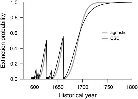
To get a better sense of how the new equation actually works and how it differs from CSD, it may be helpful to look at a small exemplary data set. Figure 1 shows posterior probabilities based on the dodo sighting record reported by Roberts and Solow (Reference Roberts and Solow2003). Three differences between the current and earlier methods are apparent.
Performance of the agnostic equation and of CSD (Alroy Reference Alroy2014) when applied to the dodo sighting record reported by Roberts and Solow (Reference Roberts and Solow2003). Small boxes show the sighting years; black line shows the agnostic posteriors; gray line shows the CSD posteriors.
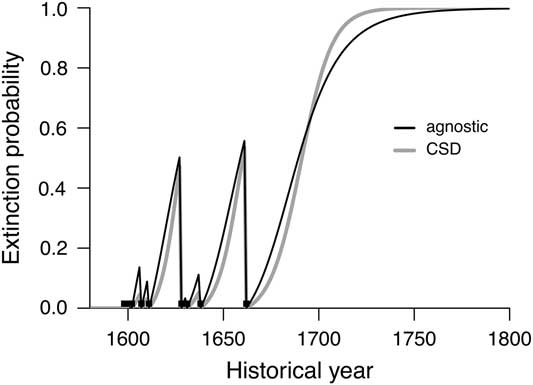
First, the new equation yields posteriors that initially climb almost linearly before plateauing, whereas CSD suggests a sigmoidal shape. The former pattern might be more intuitive, because we expect that if a species is really extinct, then the chance it was extinct in a given year should not be particularly low at the start. Or it might not: I leave the matter of intuitiveness to the reader. Regardless, the pattern stems directly from the prior assumption of an exponentially distributed extinction probability (and would be much the same on the assumption of a uniform distribution).
Second, the new method is more conservative at high values. For example, it exceeds the 0.95 level in the year 1732, whereas CSD hits this point in 1715. The equation’s conservative tendency is put forth in this paper as its main advantage.
Third, both methods yield a “best guess” value of 0.5 at about the same time: the new one reaches this threshold in 1690 and the old one in 1692. Interestingly, Roberts and Solow (Reference Roberts and Solow2003) also reported a best guess of 1690. Their figure is not truly comparable, because it represents the 0.5 confidence limit and is therefore a conditional probability instead of a posterior. The coincidence is nonetheless intriguing.
Simulations
Although it is interesting to see how the agnostic equation works, the real question is whether it works. We will therefore turn to a simulation algorithm closely modeled on that of Alroy (Reference Alroy2014), which demonstrates the new method’s accuracy with respect to computing posteriors. By default, there are 50 time intervals, the per-interval extinction probability E is 0.05, and the per-interval sampling probability p s is 0.50. The initial cohort is 1000 species, and it is assumed that all 1000 were sampled at time 0.
As mentioned, it is technically possible to compute agnostic probabilities even if there is a single sighting. Because this would be nonsense, the two-sighting cutoff is used in all the simulations reported here. By contrast, Alroy (Reference Alroy2014) excluded species with less than three sightings, because CSD probabilities are otherwise not computable.
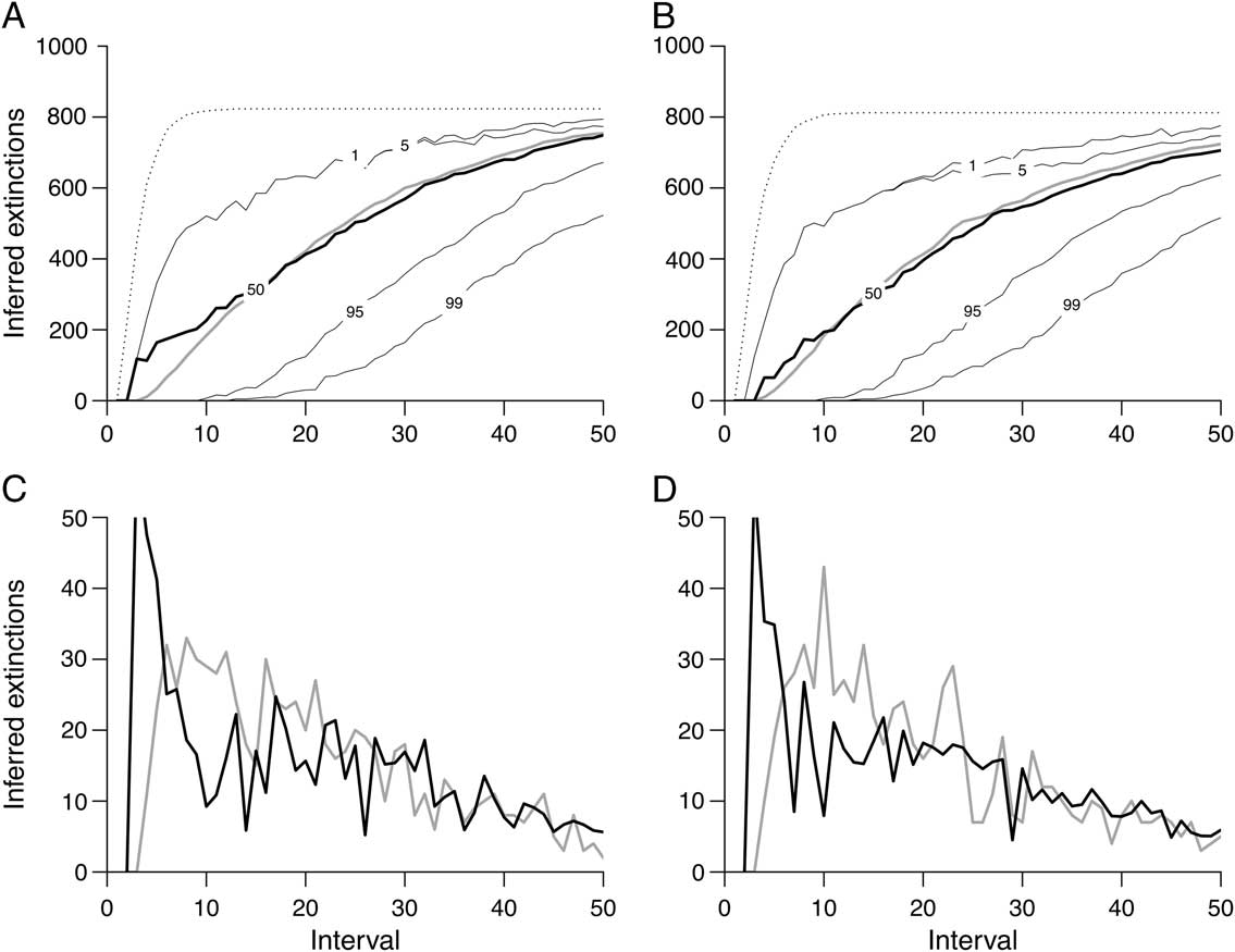
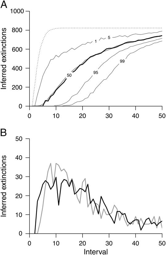
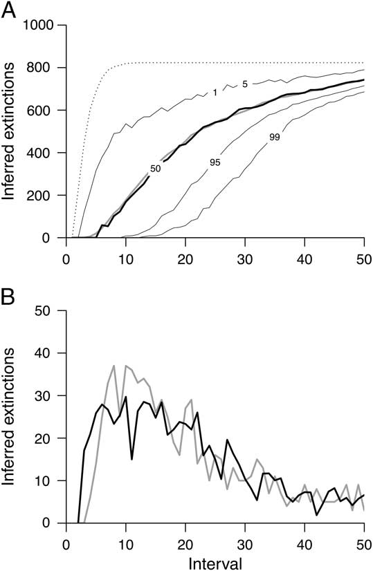
Based on the count of species with posterior extinction probabilities ε>0.50 (black line in Fig. 2), the agnostic estimates are accurate but usually very slightly downward biased relative to the true count (gray lines in Fig. 2). However, the gap seems unimportant, with the true tallies and ε>0.50 tallies being off by about 2–6% throughout most of the time series (starting from around interval 20) when one assumes that extinction probabilities are exponentially distributed (Fig. 2B). Furthermore, CSD’s performance is arguably worse (see Alroy Reference Alroy2014: Fig. 2B). The truly striking difference is that CSD very often infers ε>0.95 or even 0.99, whereas the 0.50, 0.95, and 0.99 ε lines are widely spaced in the current simulation (Fig. 2A,B). In other words, the new method is very conservative in the narrow sense of tending not to infer extinction strongly (meaning it produces few false positives) but no more or less conservative with respect to inferring survival (because the 0.01 and 0.05 lines are in about the same place in the two plots).
Performance of the agnostic equation based on a simulation analysis involving a cohort of 1000 species. The per-interval extinction probability E is 0.05 and the per-interval sampling probability p s is 0.5. The dotted line indicates the number of species that have been sampled at least twice up to this point and therefore have computable extinction probabilities; gray line, number of those that are actually extinct; thick black line labeled 50, number with posterior extinction probabilities >0.5; thin lines, number with probabilities at other cutoffs (as labeled). Compare with Figure 2B in Alroy (Reference Alroy2014). A, Results obtained by assuming a uniform distribution of extinction probabilities. B, Results obtaining by assuming an exponential distribution of extinction probabilities. C, First differences of the data shown in (A), that is, interval-by-interval rates of actual and inferred extinction. To improve visibility, the black line is based on summed posteriors instead of counts of posteriors >0.5. D, First differences of the data shown in (B). Black line is based on summed posteriors.
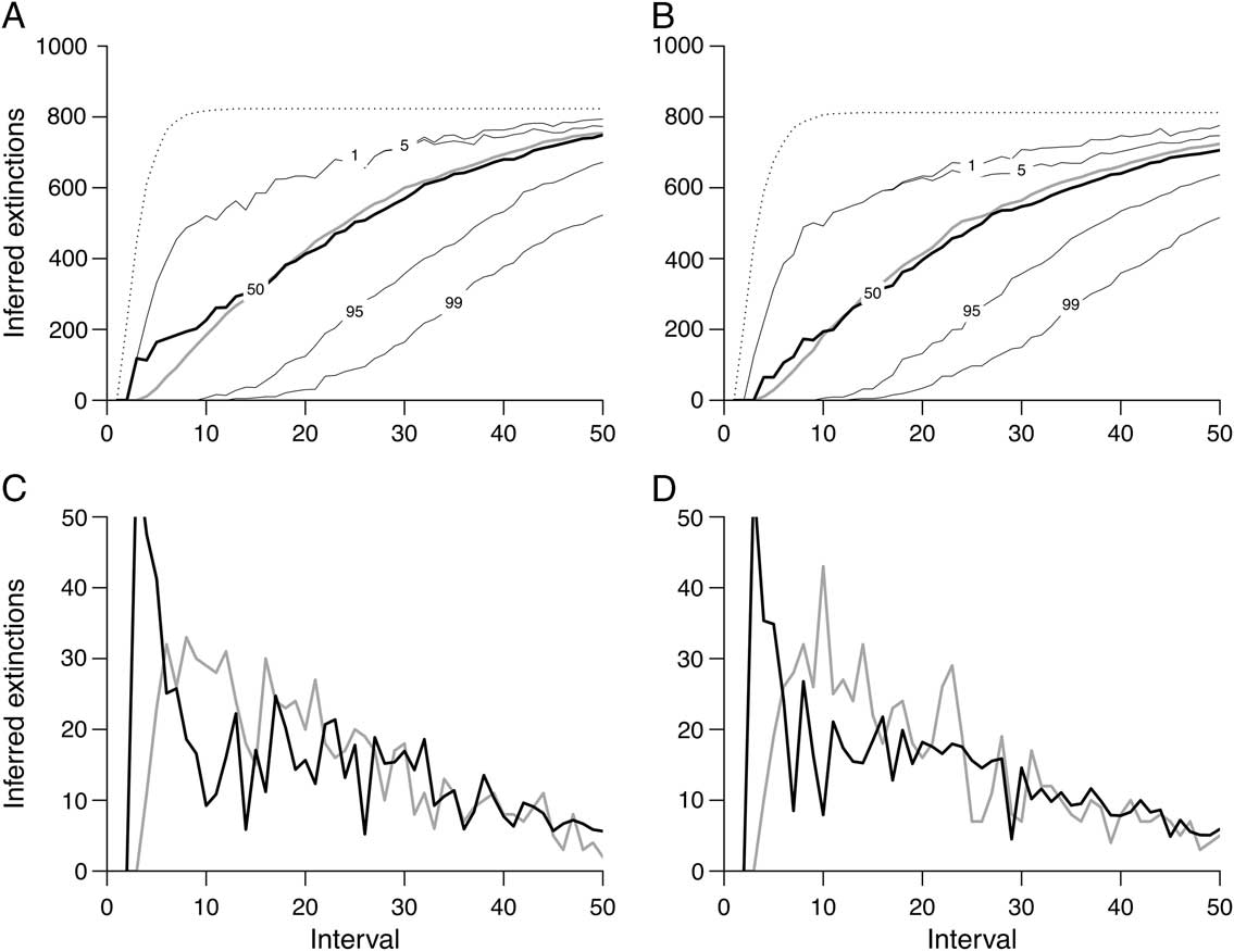
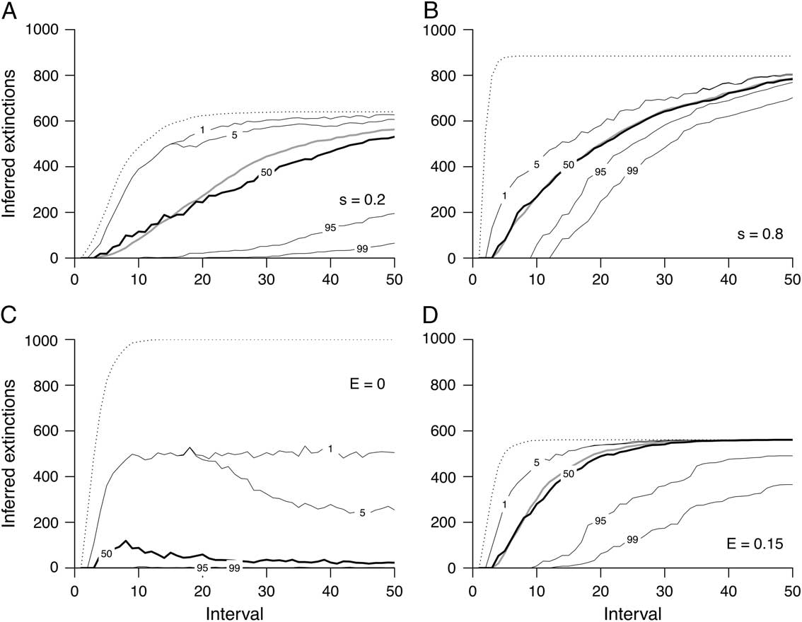
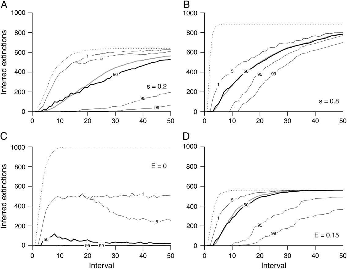
Similar patterns become evident when the sampling and extinction probabilities are varied (Fig. 3). For example, the 0.01, 0.05, and 0.50 lines are likewise about the same as with CSD when sampling is good (Fig. 3B) or extinction is rapid (Fig. 3D), but the 0.95 and 0.99 lines are again low. However, there are two key differences. First, CSD is upward biased when sampling is poor and the number of intervals is low (Alroy Reference Alroy2014: Fig. 3A, left), whereas agnostic ε values are only weakly affected in this way (left side of Fig. 3A). By contrast, they are a bit more downward biased when sampling is poor and the number of intervals is high (right side of Fig. 3A). This pattern again points to the method’s conservativeness. Second, the agnostic method has an extremely low false-positive rate when there is no extinction (Fig. 3C). More specifically, it almost never infers extinction at the 0.95 level. By implication, if ε is high for several species, then we can infer with some confidence that we are not dealing with the zero-extinction case of Figure 3C and that at least one real extinction has occurred.
Effect of varying sampling and extinction probabilities (E and p s). Lines are as in Figure 2; the legend s means p s. Compare with Figure 3 in Alroy (Reference Alroy2014). A, p s=0.2 and E=0.05. B, p s=0.8 and E=0.05. C, p s=0.5 and E=0.0. D, p s=0.5 and E=0.15.
Many other potential issues could be brought up, but because CSD and the agnostic method generally agree with respect to the ε>0.50 cutoff, there is no need to go into many more details. For example, varying the degree of temporal resolution has no effect in either case (see Alroy Reference Alroy2014: Fig. 6).
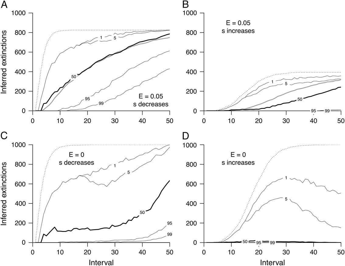
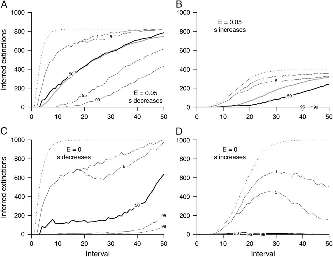
However, trends in sampling are sufficiently worrisome that it is indeed worth examining them (Fig. 4). Agnostic probabilities are even more accurate than CSD probabilities when sampling declines and extinction rates are modest (Fig. 4A); they are more strongly downward biased when sampling increases (Fig. 4B); and they are much more conservative in general when there is no extinction (Fig. 4C,D). In fact, under improving sampling and no extinction (Fig. 4D), agnostic ε values are virtually never >0.50, which is truly remarkable. The false-positive rate at the ε>0.5 level is high under decreasing sampling (Fig. 4C), but false-positive inferences at the level of ε>0.95 are negligible until sampling probabilities decline to around 0.1 or less (at about interval 40).
Effect of imposing linear sampling trends. Lines and legends are as in Figures 2 and 3. Compare with Figure 3 in the present paper and with Figure 7 in Alroy (Reference Alroy2014). A, p s decreases from 0.5 to 0 and E=0.05. B, p s increases from 0 to 0.5 and E=0.05. C, p s decreases from 0.5 to 0 and E=0. D, p s increases from 0 to 0.5 and E=0.
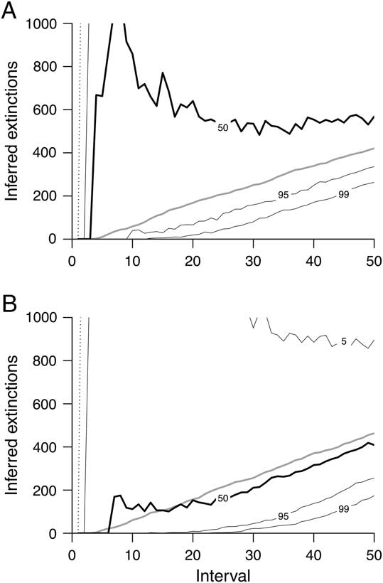
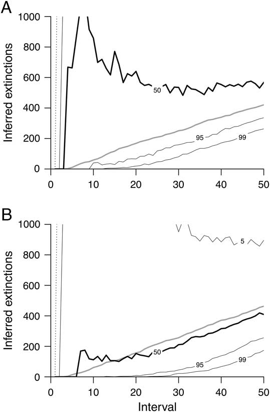
One final consideration is the method of recycling posteriors as priors based on population means. Applying this method to the standard simulation model greatly improves the fit (Fig. 5 vs. Fig. 2B,D). Furthermore, a simulation with a suitably large species pool of 10,000 and a quite low per-interval extinction rate of 0.001 demonstrates that this technique yields more accurate results even in extreme circumstances: it is a bit downward biased (Fig. 6B) instead of quite considerably upward biased (Fig. 6A). However, the amount of random sampling error is great enough when dealing with tiny extinction probabilities that recycling cannot be recommended unless the data set is indeed large. Also, recycling is not absolutely necessary unless the extinction rate is quite low, because a 0.5 prior yields highly accurate estimates given moderate extinction rates (Fig. 2). Based on varying combinations of the simulation parameters, a good rule of the thumb seems to be that recycling is feasible and sensible if at least several scores of species are being analyzed. Few paleontological data sets will meet this description, but neontological data sets might do so in cases where a major taxonomic group is being assessed using a very large catalogue of museum specimens (as in Alroy Reference Alroy2015).
Effect of recycling posteriors given near-zero extinction rates. There are 10,000 species, p s=0.5, and E=0.001. A, Results obtained using the standard method. B, Results obtained by recycling.
Conclusions
The agnostic equation is highly distinctive for two closely related reasons: it has an extremely low false-positive rate (Figs. 3C and 4C,D) and it rarely produces a near-one extinction probability unless sampling is fairly intensive, sampling trends downward or is flat, and the extinction rate is well above zero (Figs. 1, 3B,D, and 4A). Conversely, under such circumstances the new method produces near-zero probabilities at pretty much the same rate as CSD.
We might then ask why anyone would favor such a stubbornly conservative method. The reason is that although one always wishes to obtain an accurate estimate of the total number of extinctions, inferring extinction in any one case may be costly. A good analogy is the life insurance industry. Inferring any one death is literally costly and therefore to be avoided, but correctly figuring the total number of deaths is crucially important for the purpose of determining premiums. The new method accomplishes both goals. In a biological context, it is therefore probably most useful for assessing endangered species: strong conservation efforts are particularly mandated whenever the status of a species is uncertain, making it imperative that a fair and not extreme number be put on the chance of extinction to date. Conservativeness in the form of indecisiveness is important in any such context.
Acknowledgments
I thank A. Solow for pointing me to the key contribution of Höhle and Held (Reference Höhle and Held2006), which led me to Goodman (Reference Goodman1952).