1 Background
It has been known for over 100 years that two distinct nested and unlinked ideal vortex rings will leapfrog through one another as they propagate downstream, with the inner ring becoming the outer ring and the outer ring becoming the inner ring.
How would this interaction be modified if the rings were coiled? Would the rings reconnect instead of leapfrogging, and what diagnostics should be used? Scheeler et al. (Reference Scheeler, van Rees, Kedia, Kleckner and Irvine2017) has recently shown how to experimentally generate coiled vortex rings and claim that they can follow the evolution of the rings’ discrete topological properties. This includes their twist
 $Tw$
, writhe
 $Wr$
and self-linking
 ${\mathcal{L}}_{S}$
numbers (2.12), along with their centreline helicities
 ${\mathcal{H}}_{cj}$
(2.14). This could be an important advance and would provide evidence on the roles of topology, reconnection and helicity in the evolution of turbulence.
However, independent validation is required for the claim that their experiments can preserve the total helicity/self-linking
 ${\mathcal{L}}_{S}$
, despite large transfers between
 $Wr$
and
 $Tw$
, and still satisfy
 $$\begin{eqnarray}{\mathcal{L}}_{S}=Tw+Wr,\end{eqnarray}$$
a constraint introduced by Calugareanu (Reference Calugareanu1959) with a simplified proof by Pohl (Reference Pohl1968). The concern is that only
 $Wr$
and the
 ${\mathcal{H}}_{cj}$
are measured, with
 ${\mathcal{L}}_{S}$
obtained by assuming that
 ${\mathcal{H}}=\sum _{j}{\mathcal{H}}_{cj}$
and (1.2). Then (1.1) is used to find
 $Tw$
, instead of being using to validate the
 $Tw$
,
 $Wr$
and
 ${\mathcal{L}}_{S}$
results.
A known test that immediately shows that one or more of their
 $Tw$
,
 $Wr$
and
 ${\mathcal{L}}_{S}$
results are incorrect is to independently determine all three numbers from the analytic closed trajectories (2.7) of Scheeler et al. (Reference Scheeler, van Rees, Kedia, Kleckner and Irvine2017). This can be done using the algorithms of Moffatt & Ricca (Reference Moffatt and Ricca1992) and shows that each topological number for the coil trajectories is positive with
 $Tw\gg Wr$
, not
 $Tw\ll Wr$
, raising questions about whether there is a physical role for the topological helicity:
 $$\begin{eqnarray}{\mathcal{H}}_{T}=\mathop{\sum }_{i\neq j}\unicode[STIX]{x1D6E4}_{i}\unicode[STIX]{x1D6E4}_{j}{\mathcal{L}}_{ij}+\mathop{\sum }_{j}\unicode[STIX]{x1D6E4}_{j}^{2}{\mathcal{L}}_{S_{j}},\end{eqnarray}$$
where the
 $\unicode[STIX]{x1D6E4}_{j}$
are the circulations of the vortices (2.10). Experimental and numerical trefoil vortex knots have found that during reconnection
 ${\mathcal{H}}_{T}$
is preserved, along with some exchange of linking between the writhe and twist (Scheeler et al.
Reference Scheeler, Kleckner, Proment, Kindlmann and Irvine2014; Kerr Reference Kerr2018a
,Reference Kerr
b
). However, the trefoils are a unique, extremely helical configuration. To determine whether the topological numbers consistently have roles in the dynamics of reconnection and the flow of turbulent energy to small scales, identifying those numbers correctly for less helical configurations such as coiled rings is essential.
Once the
 $Tw$
,
 $Wr$
and
 ${\mathcal{L}}_{S}$
discrepancies in the Scheeler et al. (Reference Scheeler, van Rees, Kedia, Kleckner and Irvine2017) results were recognised, numerics were begun to help determine which of the inferred topological numbers are correct and what, if any, physical roles they might play. These numerical methods have previously been validated by comparisons with experiments, the reconnecting trefoil vortex knots of Kleckner & Irvine (Reference Kleckner and Irvine2013), and used to obtain run-time values for
 $Wr$
and
 ${\mathcal{L}}_{S}$
(Kerr Reference Kerr2018a
). This paper complements those topological diagnostics with an improved algorithm for calculating the twist
 $Tw$
(2.12) from the Frenet–Serret relations (2.11) that now is accurate enough to allow validation of all three topological numbers using (1.1).
The bottom line for the Scheeler et al. (Reference Scheeler, van Rees, Kedia, Kleckner and Irvine2017) experimental topological numbers is that the new diagnostics and numerics confirm only the values of the
 $t=0$
writhe
 $Wr$
, and none of their reported
 $Tw$
,
 ${\mathcal{L}}_{S}$
and
 ${\mathcal{H}}_{c}$
values. In particular, their claim that linking is exchanged between
 $Wr$
and
 $Tw$
with
 $Wr\gg Tw$
is not confirmed. In contrast,
 $Wr\ll Tw$
, all the helicities are much smaller than the predictions of (1.2) and neither
 $Wr$
nor
 $Tw$
changes significantly before reconnection ends.
Despite being static during reconnection, in this new picture the topological numbers
 $Wr$
and
 $Tw$
retain important complementary roles in the dynamics of the global helicity
 ${\mathcal{H}}$
(2.4) and enstrophy
 $Z$
(2.3) – dynamics that show the beginnings of a cascade to small scales. Specifically, it is
 $Wr$
that controls the
 ${\mathcal{H}}_{c}$
, and hence
 ${\mathcal{H}}$
, values, not the self-linking
 ${\mathcal{L}}_{S}$
, with
 $$\begin{eqnarray}{\mathcal{H}}\approx {\mathcal{H}}_{c}\sim (\text{1 to 2})Wr\unicode[STIX]{x1D6E4}^{2}\ll {\mathcal{L}}_{S}\unicode[STIX]{x1D6E4}^{2}.\end{eqnarray}$$
While the growth of the enstrophy
 $Z$
, given later in figure 6, could be tied to the development of small scales in the
 $s$
-profiles of the torsion
 $\unicode[STIX]{x1D70F}$
given in figure 3, and whose
 $s$
-integrals are the twist (2.12). The axial velocity profiles in 3 also provide clues to the surprisingly small experimental
 ${\mathcal{H}}_{c}$
in Scheeler et al. (Reference Scheeler, van Rees, Kedia, Kleckner and Irvine2017), with values smaller than even those from (1.3).
The remainder of this paper is organised as follows. First, there is a summary of the underlying continuum equations, the diagnostics and the steps used to generate the numerical coiled rings. The results begin with single rings with single coils to illustrate the relationship between the linking and helicity diagnostics and the number and size of the coils. Then the time-evolving, nested two-ring cases are presented, with the focus upon cases with five coils on the inner ring, because all of their topological diagnostics can be determined and validated and they have the cleanest
 $Z^{-1/2}$
enstrophy scaling. Besides comparing the experimental writhes
 $Wr$
at
 $t=0$
, validation that these calculations represent the dynamics of the experimental coiled rings will come from the time scales over which the rings move in and about
 $z$
and begin to swap positions. The temporal evolution and scaling of the continuum helicity
 ${\mathcal{H}}$
and enstrophy
 $Z$
are then related to how they behave in recent trefoil and anti-parallel reconnection calculations. Finally, how these numerical methods could determine the topological numbers of experimental vortices is noted.
2 Equations: continuum, initial states and diagnostics
The governing equations for the simulations of the velocity
 $\boldsymbol{u}$
are the incompressible Navier–Stokes equations with viscosity
 $\unicode[STIX]{x1D708}$
in a periodic box with volume (
 $V=\ell ^{3}$
).
 $$\begin{eqnarray}\left.\begin{array}{@{}r@{}}\displaystyle \boldsymbol{u}_{t}-\unicode[STIX]{x1D708}\unicode[STIX]{x0394}\boldsymbol{u}+(\boldsymbol{u}\boldsymbol{\cdot }\unicode[STIX]{x1D735})\boldsymbol{u}+\unicode[STIX]{x1D735}p=0,\\ \displaystyle \unicode[STIX]{x1D735}\boldsymbol{\cdot }\boldsymbol{u}=0,\end{array}\right\}\quad \text{in}~\mathbb{T}_{\ell }^{3}\times [0,T).\end{eqnarray}$$
The vorticity
 $\unicode[STIX]{x1D74E}(\boldsymbol{x})=\unicode[STIX]{x1D735}\times \boldsymbol{u}(\boldsymbol{x})$
equation is
 $$\begin{eqnarray}\frac{\unicode[STIX]{x2202}\unicode[STIX]{x1D74E}}{\unicode[STIX]{x2202}t}+(\boldsymbol{u}\boldsymbol{\cdot }\unicode[STIX]{x1D735})\unicode[STIX]{x1D74E}=(\unicode[STIX]{x1D74E}\boldsymbol{\cdot }\unicode[STIX]{x1D735})\boldsymbol{u}+\unicode[STIX]{x1D708}\unicode[STIX]{x0394}\unicode[STIX]{x1D74E},\quad \unicode[STIX]{x1D735}\boldsymbol{\cdot }\unicode[STIX]{x1D74E}=0.\end{eqnarray}$$
The enstrophy density
 $|\unicode[STIX]{x1D74E}|^{2}$
equation and the volume-integrated enstrophy
 $Z$
are
 $$\begin{eqnarray}\frac{\unicode[STIX]{x2202}|\unicode[STIX]{x1D74E}|^{2}}{\unicode[STIX]{x2202}t}+(\boldsymbol{u}\boldsymbol{\cdot }\unicode[STIX]{x1D735})|\unicode[STIX]{x1D74E}|^{2}=\underbrace{2\unicode[STIX]{x1D74E}\boldsymbol{S}\unicode[STIX]{x1D74E}}_{Z_{p}=production}+\unicode[STIX]{x1D708}\unicode[STIX]{x0394}|\unicode[STIX]{x1D74E}|^{2}-\underbrace{2\unicode[STIX]{x1D708}(\unicode[STIX]{x1D735}\unicode[STIX]{x1D74E})^{2}}_{\unicode[STIX]{x1D716}_{\unicode[STIX]{x1D714}}=Z-dissipation},\quad Z=\int \unicode[STIX]{x1D74E}^{2}\,\text{d}V,\end{eqnarray}$$
where
 $\boldsymbol{S}=(1/2)(\unicode[STIX]{x1D735}\boldsymbol{u}+\unicode[STIX]{x1D735}\boldsymbol{u}^{\text{T}})$
is the strain and the normalised enstrophy production rate or velocity-derivative skewness is
 $-S_{u}=D\unicode[STIX]{x1D74E}\boldsymbol{S}\unicode[STIX]{x1D74E}/Z^{3/2}$
. The equation for helicity density
 $h$
is
 $$\begin{eqnarray}\frac{\unicode[STIX]{x2202}h}{\unicode[STIX]{x2202}t}+(\boldsymbol{u}\boldsymbol{\cdot }\unicode[STIX]{x1D735})h=\underbrace{-\unicode[STIX]{x1D74E}\boldsymbol{\cdot }\unicode[STIX]{x1D735}\unicode[STIX]{x1D6F1}}_{\unicode[STIX]{x1D714}-transport}+\underbrace{\unicode[STIX]{x1D708}\unicode[STIX]{x0394}h}_{\unicode[STIX]{x1D708}-transport}-\underbrace{2\unicode[STIX]{x1D708}\text{tr}(\unicode[STIX]{x1D735}\unicode[STIX]{x1D74E}\boldsymbol{\cdot }\unicode[STIX]{x1D735}\boldsymbol{u}^{\text{T}})}_{\unicode[STIX]{x1D716}_{h}={\mathcal{H}}-dissipation},\quad {\mathcal{H}}=\int \boldsymbol{u}\boldsymbol{\cdot }\unicode[STIX]{x1D74E}\,\text{d}V,\end{eqnarray}$$
where
 $\unicode[STIX]{x1D6F1}=p-(1/2)\boldsymbol{u}^{2}\neq p_{h}$
, the pressure head
 $p_{h}=p+(1/2)\boldsymbol{u}^{2}$
, and
 ${\mathcal{H}}$
is the global helicity.
An alternative way to formulate incompressible velocity and vorticity fields is the Clebsch decomposition, which, under Euler, can be defined by pairs of advected scalar fields
 $(a_{j}(\boldsymbol{x}),b_{j}(\boldsymbol{x}))$
, for which the incompressible velocity and vorticity fields are
 $$\begin{eqnarray}\boldsymbol{u}=\mathop{\sum }_{j}a_{j}\unicode[STIX]{x1D735}b_{j}+\unicode[STIX]{x1D735}\unicode[STIX]{x1D719}\quad \text{and}\quad \unicode[STIX]{x1D74E}=\mathop{\sum }_{j}\unicode[STIX]{x1D735}b_{j}\times \unicode[STIX]{x1D735}a_{j},\end{eqnarray}$$
where the extra
 $\unicode[STIX]{x1D719}(\boldsymbol{x})$
potential imposes incompressibility and whose
 $\unicode[STIX]{x1D74E}$
is similar to the definition of a pseudovorticity for a quantum fluid (Rorai et al.
Reference Rorai, Skipper, Kerr and Sreenivasan2016). By applying integration by parts to the
 $\unicode[STIX]{x1D735}\unicode[STIX]{x1D719}$
term one can show that the global self-helicity for a single pair
 $(a_{1},b_{1})$
is identically zero:
 $$\begin{eqnarray}{\mathcal{H}}_{S}=\int (\boldsymbol{u}_{1}\times \unicode[STIX]{x1D74E}_{1})\,\text{d}V\equiv 0,\end{eqnarray}$$
an identity that implies that at least two Clebsch pairs are required for there to be finite hydrodynamic helicity
 ${\mathcal{H}}$
and represents a fundamental difference between the magnetic helicity, defined as
 ${\mathcal{H}}_{M}=\int \boldsymbol{A}\boldsymbol{\cdot }\boldsymbol{B}\,\text{d}V$
with
 $\unicode[STIX]{x1D735}\boldsymbol{\cdot }\boldsymbol{A}$
unspecified, and the
 $\unicode[STIX]{x1D735}\boldsymbol{\cdot }\boldsymbol{u}\equiv 0$
hydrodynamic helicity. Examples of configurations with finite helicity are linked rings, with each ring defined by its own Clebsch pair such that the helicity of their coupled velocities and vorticities is
 $2{\mathcal{L}}_{12}\unicode[STIX]{x1D6E4}_{1}\unicode[STIX]{x1D6E4}_{2}$
. For the trefoil initialisation in Kerr (Reference Kerr2018a
), which gives
 ${\mathcal{H}}/\unicode[STIX]{x1D6E4}^{2}\equiv {\mathcal{L}}_{S}=3$
, a second Clebsch pair should exist because two points from the trefoil were used to generate the vorticity at each mesh point. However, the coiled rings do not have an obvious second Clebsch pair, so (1.2) does not have to be obeyed.
2.1 Summary of the calculations
The initial trajectories of the coiled rings
 $\boldsymbol{X}_{h}(\unicode[STIX]{x1D719})=(x,y,z)$
are:
 $$\begin{eqnarray}\left.\begin{array}{@{}r@{}}x(\unicode[STIX]{x1D719})=R(\unicode[STIX]{x1D719})\cos (\unicode[STIX]{x1D719}),\quad y(\unicode[STIX]{x1D719})=R(\unicode[STIX]{x1D719})\sin (\unicode[STIX]{x1D719}),\quad z(\unicode[STIX]{x1D719})=A(\unicode[STIX]{x1D719})\cos (m\unicode[STIX]{x1D719})\\ \quad \text{where }R(\unicode[STIX]{x1D719})=R_{h}+A(\unicode[STIX]{x1D719})\sin (m\unicode[STIX]{x1D719})\quad \text{with}~\unicode[STIX]{x1D719}=[1:2\unicode[STIX]{x03C0}].\end{array}\right\}\end{eqnarray}$$
For all the
 $m\neq 1$
cases,
 $R_{h}$
and
 $A(\unicode[STIX]{x1D719})$
are the values used by Scheeler et al. (Reference Scheeler, van Rees, Kedia, Kleckner and Irvine2017)
Once all the trajectories are defined, vortices of finite radii are mapped onto the mesh (Kerr Reference Kerr2013). First, a preliminary field of two superposed vortex rings
 $\unicode[STIX]{x1D74E}_{j}(\boldsymbol{x})$
,
 $j\in [1,2]$
, is generated using the Rosenhead regularisation of a point vortex (2.8) with radii of
 $a_{0}$
, multiplied by the tangent
 $\boldsymbol{T}_{j}(\unicode[STIX]{x1D719})$
(2.11) at
 $\boldsymbol{x}_{j}(\unicode[STIX]{x1D719})$
:
 $\unicode[STIX]{x1D74E}_{j}(\boldsymbol{x}_{j})=|\unicode[STIX]{x1D714}_{j}(\boldsymbol{x}_{j})|\boldsymbol{T}_{j}(\unicode[STIX]{x1D719})$
, where
 $r=|\boldsymbol{x}-\boldsymbol{x}_{j}(\unicode[STIX]{x1D719})|$
and
 $\boldsymbol{x}_{j}(\unicode[STIX]{x1D719})$
is the nearest point on the coiled ring. This and the next step use
 $$\begin{eqnarray}|\unicode[STIX]{x1D714}_{j}|(\boldsymbol{x})=\unicode[STIX]{x1D6E4}\frac{(a_{0}^{2})}{(r^{2}+a_{0}^{2})^{2}},\quad \tilde{\unicode[STIX]{x1D74E}}_{f}(\boldsymbol{k})=\tilde{\unicode[STIX]{x1D74E}}_{i}(\boldsymbol{k})\exp \left(-\frac{k^{4}}{k_{f}^{4}}\right)\quad \text{and}\quad a_{e}=\left(\frac{\unicode[STIX]{x1D6E4}}{\unicode[STIX]{x1D714}_{0}\unicode[STIX]{x03C0}}\right)^{1/2},\end{eqnarray}$$
where the
 $k_{f}$
hyperviscous smoothing is applied to the preliminary Fourier transformed
 $\tilde{\unicode[STIX]{x1D74E}}_{i}(\boldsymbol{k})$
field to get
 $\tilde{\unicode[STIX]{x1D74E}}_{f}(\boldsymbol{k})$
. Incompressibility is then applied before the Fourier fields are transformed back to give a final
 $\boldsymbol{u}(\boldsymbol{x})|_{t=0}$
field. The vortices of the initial coiled rings all have a circulation of
 $\unicode[STIX]{x1D6E4}=1720$
and, after the smoothing, their effective radii have increased to
 $a_{e}\approx 1.2a_{0}=21.6$
, with their initial peak vorticities adjusted to be
 $\unicode[STIX]{x1D714}_{0}\approx 1$
.
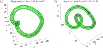
Two single rings with a single coil, both initialised on
 $256^{3}$
meshes. (a) Case
 $\text{s}_{a}$
has a single, small coil with
 ${\mathcal{H}}/\unicode[STIX]{x1D6E4}^{2}=0.3$
(from
 ${\mathcal{H}}_{0}=8.6\times 10^{5}$
and
 $\unicode[STIX]{x1D6E4}^{2}=2.8\times 10^{6}$
) and is twist-dominated, with
 $Tw=0.67$
,
 $Wr=0.33$
and
 ${\mathcal{L}}_{S}=1$
, like all the multicoiled rings used for the nested ring calculations. (b) Case s
 $_{b}$
has a single midsized, writhe-dominated coil with
 ${\mathcal{H}}/\unicode[STIX]{x1D6E4}^{2}=0.53$
(from
 ${\mathcal{H}}_{0}=1.6\times 10^{6}$
and
 $\unicode[STIX]{x1D6E4}^{2}=3\times 10^{6}$
),
 $Tw=0.29$
,
 $Wr=0.71$
and
 ${\mathcal{L}}_{S}=1$
.

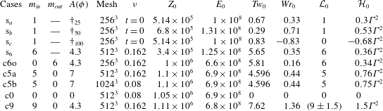
Viscosities and parameters for the initial conditions using (2.8). All the calculations were done in
 $(144\unicode[STIX]{x03C0})^{3}\approx 452^{3}$
domains with the radius of the inner (or only) ring in each case
 $R_{h\text{-}in}=72$
and the outer ring
 $R_{h\text{-}out}=120$
with
 $A(\unicode[STIX]{x1D719})$
in (2.7) constant except for (below) s
 $_{a,b,c}$
. Mesh
 $=$
the final computational mesh. For all the cases
 $a_{0}=18$
and
 $k_{f}=84$
in (2.8), giving effective radii of
 $a_{e}=21.6$
, circulations of
 $\unicode[STIX]{x1D6E4}=1720$
, and
 $\unicode[STIX]{x1D714}_{0}=1.08$
, except for the case c9, whose
 $\unicode[STIX]{x1D714}_{0}=1.14$
and whose
 ${\mathcal{L}}_{S}$
is uncertain, varying with
 $\unicode[STIX]{x0394}{\mathcal{L}}_{S}=\pm 1.5$
for
 $\unicode[STIX]{x1D6FF}=0.09\pm 0.025$
with
 $\unicode[STIX]{x1D700}=0.18$
in (2.13). The
 $t=0$
global enstrophies
 $Z_{0}$
, energies
 $E_{0}$
and helicities are given. For s
 $_{a}$
(
 $\dagger _{25}$
) the trajectory is
 $A(\unicode[STIX]{x1D719})=25((1-\sin \unicode[STIX]{x1D719})^{2}-(1-\sin \unicode[STIX]{x1D719}))$
and for s
 $_{b}$
(
 $\dagger _{50}$
) and s
 $_{c}$
(
 $\dagger _{100}$
):
 $a(\unicode[STIX]{x1D719})=a_{f}(1-\sin \unicode[STIX]{x1D719})$
for
 $a_{f}=50$
and 100. For the
 $\unicode[STIX]{x1D708}=0.16$
cases, the Reynolds number of
 $Re=\unicode[STIX]{x1D6E4}/\unicode[STIX]{x1D708}=10\,000$
is comparable to the experimental values of
 $Re=12\,000{-}20\,000$
.

The initial conditions, including the initial twist
 $Tw_{0}$
, writhe
 $Wr_{0}$
and global helicities
 ${\mathcal{H}}_{0}$
, for all of the simulations are given in table 1. The single-ring cases demonstrate the range of
 $Tw$
and writhe
 $Wr$
generated by different trajectories and how they contribute to the continuum helicities
 ${\mathcal{H}}$
. The multicoil cases are a single ring with six coils, a nested pair with a six-coil outer ring and two nested pairs with inner ring coils, one with five coils and one with nine. The centreline trajectories of the six- and nine-coil cases are given by the experimental hydrofoils (Scheeler et al.
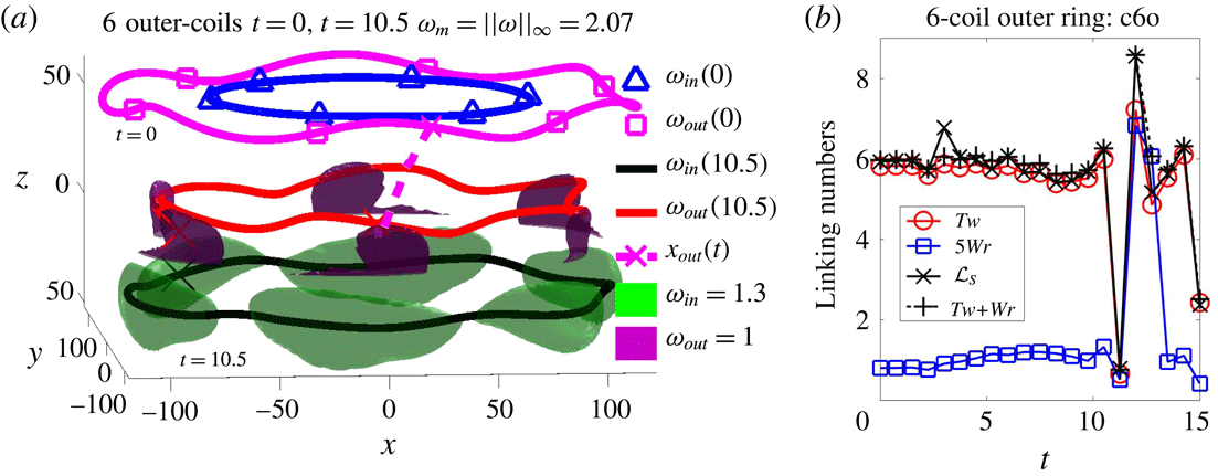
Reference Scheeler, van Rees, Kedia, Kleckner and Irvine2017). The rings are visualised using vorticity isosurfaces and centreline vortices within those isosurfaces in figures 1, 2(a) and 4(a).
Validation that the computational coiled vortices represent the new ring experiments is done in two ways. One is the values of the
 $t=0$
writhe. The other validation is, as in Kerr (Reference Kerr2018a
), to scale the rings’ evolution by the nonlinear time and velocity scales,
 $$\begin{eqnarray}t_{\unicode[STIX]{x1D6E4}}=R_{e}^{2}/\unicode[STIX]{x1D6E4}\quad \text{and}\quad U_{z}\sim \unicode[STIX]{x1D6E4}/R_{e},\end{eqnarray}$$
where
 $R_{e}$
is the average radii of the vortex rings. This allows comparisons between the times at which the numerical and experimental rings pass one another and how far the rings have propagated by those times.
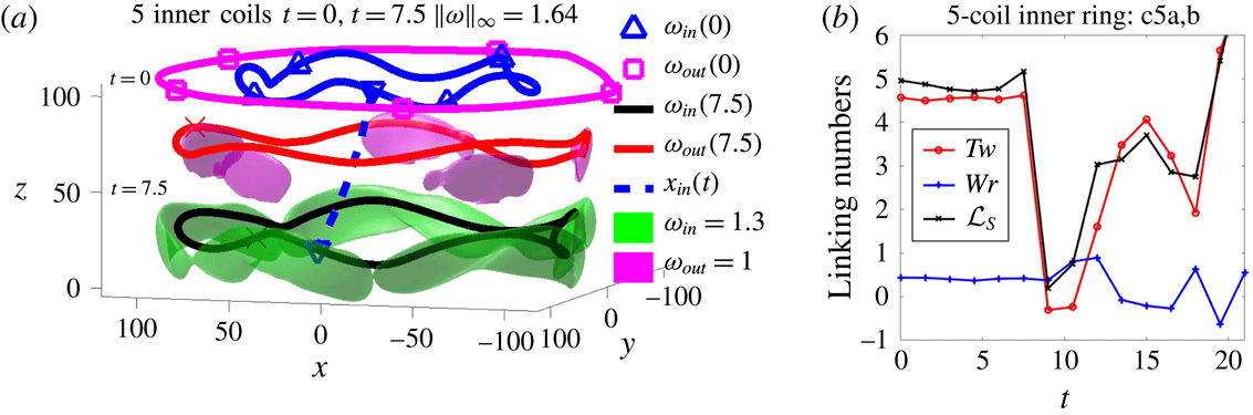
(a) Visualisation of case c5, two rings whose inner ring has five coils. The
 $t=0$
centreline vortices are indicated at the top by the curves with ▫ and ▵ symbols. Centreline vortices passing through two isosurfaces at
 $t=7.5$
show the configuration as reconnection ends. The blue-dashed curve indicates the Lagrangian motion
 $\boldsymbol{x}_{in}(s_{c},t)$
of a point (
 $s_{c}$
) on one of the inner coils whose velocity (3.1) is
 $(u_{\unicode[STIX]{x1D719}\text{-}in},u_{z\text{-}in})\approx (10.3,-10.9)$
as it moves to the outside of the magenta uncoiled ring. (b) Evolution of
 $Tw$
,
 $Wr$
and
 ${\mathcal{L}}_{S}\sim Tw(t)$
, which are all relatively constant until the rings interact, partially reconnect and swap positions at
 $t_{q}\approx 7.5$
. To compare to the experimental times, scaling using (2.9) gives
 $t_{q}/t_{\unicode[STIX]{x1D6E4}}\approx 1.4$
for case c5a, with the experimental time scales given after (2.15).

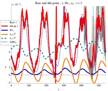
For case c5a, profiles of the torsion
 $\unicode[STIX]{x1D70F}$
,
 $s$
-gradient of the writhe
 $Wr_{s}$
, and weighted velocities
 $u_{\unicode[STIX]{x1D714}}/\unicode[STIX]{x1D6E4}$
and
 $u_{\bot }/\unicode[STIX]{x1D6E4}=|\boldsymbol{u}-u_{\unicode[STIX]{x1D714}}\boldsymbol{T}|/\unicode[STIX]{x1D6E4}$
.
 $\unicode[STIX]{x1D70F}$
is calculated using only every fourth point (red) to control the large fluctuations generated by the raw data (black with only
 $s>400$
shown).
 $10Wr_{s}$
follows
 $\unicode[STIX]{x1D70F}$
, but the
 $u_{\unicode[STIX]{x1D714}}/\unicode[STIX]{x1D6E4}$
that contribute to
 ${\mathcal{H}}_{c}$
(2.14) have stronger variations, including
 $u_{\unicode[STIX]{x1D714}}/\unicode[STIX]{x1D6E4}<0$
.
 ${\mathcal{H}}_{c}/(\unicode[STIX]{x1D6E4}^{2}Wr)=\int \text{d}s\,u_{\unicode[STIX]{x1D714}}/(\unicode[STIX]{x1D6E4}Wr)=1.4>1$
, similar to
 ${\mathcal{H}}/Wr\unicode[STIX]{x1D6E4}^{2}$
in figure 5. The perpendicular velocities on the trajectories
 $u_{\bot }/\unicode[STIX]{x1D6E4}$
are on the order of
 $|U_{z}|$
.

c6o, with a 6-coil outer ring. (a) At the top are
 $t=0$
centreline vortices (▫, ▵) and at the bottom are
 $t_{q}=10.5$
isosurfaces with centreline vortices that show the configuration as reconnection ends. Dashes show the
 $\boldsymbol{x}_{out}(s_{c},t)$
motion (3.1) of an outer coil (
 $s_{c}$
) as that ring moves inside the
 $t=0$
uncoiled ring. (b) Evolution of
 $Tw$
,
 $Wr$
and
 ${\mathcal{L}}_{S}$
, which are almost constant until the rings interact and partially reconnect at
 $t_{q}\approx 10.5$
when they swap positions in (a). The scaled reconnection/swapping time is
 $t_{q}/t_{\unicode[STIX]{x1D6E4}}\approx 1.95$
(2.9).

The calculations use the same filtered pseudospectral method (Kerr Reference Kerr2013) as the trefoil calculations, with that experience used to guide the choice of
 $\unicode[STIX]{x1D708}$
for the given ratios of the vortex thicknesses to the resolution. The one proper resolution test is cases c5a and c5b, which were run on both
 $512^{3}$
and
 $1024^{3}$
meshes, at different viscosities,
 $\unicode[STIX]{x1D708}=0.162$
and 0.08, for which the small increases in
 $\Vert \unicode[STIX]{x1D714}\Vert _{\infty }$
as
 $\unicode[STIX]{x1D708}$
decreased and resolution improved were consistent with those observed at early times in Kerr (Reference Kerr2018b
).
2.2 Vortex line diagnostics
Once the three-dimensional simulations have been run, for the two
 $j\in [1,2]$
vortex rings, one coiled, the positions
 $\boldsymbol{x}_{j}(s_{j},t)$
of their centreline vortices can be identified by applying the stream3 function in Matlab to seed points
 $\boldsymbol{x}_{j}(s=0)$
at, or near, local vorticity maxima:
 $$\begin{eqnarray}\frac{\text{d}\boldsymbol{x}_{j}(s)}{\text{d}s}=\unicode[STIX]{x1D74E}(\boldsymbol{x}_{j}(s))\quad \text{with circulations given by }\unicode[STIX]{x1D6E4}_{j}=\oint _{{\mathcal{D}}_{j}}\boldsymbol{u}_{j}\boldsymbol{\cdot }\text{d}\boldsymbol{r}_{j},\end{eqnarray}$$
where the
 $\boldsymbol{r}_{j}\in {\mathcal{D}}_{j}$
are taken about the
 $\boldsymbol{x}_{j}(s)$
. The
 $\boldsymbol{x}_{j}(s)$
curves, which tend to have thousands of points, rarely close exactly upon themselves. To get closed curves, stream3 is run in opposite directions from the local
 $\unicode[STIX]{x1D714}$
maxima, giving curves that nearly meet on the opposite side of the rings from their
 $\boldsymbol{x}_{j}(s=0)$
. These are then linearly blended using 128 points on either side of where they nearly meet to produce closed rings.
Given there are closed curves, the topological numbers
 $Tw$
,
 $Wr$
and
 ${\mathcal{L}}_{S}$
can, in principle, be found using the Frenet–Serret relations
 $$\begin{eqnarray}\boldsymbol{T}_{j}=\unicode[STIX]{x2202}_{s}\boldsymbol{x}_{j}/|\unicode[STIX]{x2202}_{s}\boldsymbol{x}_{j}|;\quad \unicode[STIX]{x1D705}\boldsymbol{N}_{j}=\unicode[STIX]{x2202}_{s}\boldsymbol{T}_{j};\quad \unicode[STIX]{x1D70F}\boldsymbol{B}_{j}-\unicode[STIX]{x1D705}\boldsymbol{T}_{j}=\unicode[STIX]{x2202}_{s}\boldsymbol{N};\quad \unicode[STIX]{x1D70F}\boldsymbol{N}_{j}=-\unicode[STIX]{x2202}_{s}\boldsymbol{B}_{j};\end{eqnarray}$$
for which the twist given in principle by
 $$\begin{eqnarray}Tw_{j}=\frac{1}{2\unicode[STIX]{x03C0}}\oint \unicode[STIX]{x1D70F}\,\text{d}s,\quad \text{using }\unicode[STIX]{x1D70F}=\frac{\text{d}\boldsymbol{N}}{\text{d}s}\boldsymbol{\cdot }\boldsymbol{B}\end{eqnarray}$$
with
 ${\mathcal{L}}_{Sj}$
and
 $Wr_{j}$
determined by regularised Gauss linking integrals between loops
 $$\begin{eqnarray}{\mathcal{L}}_{jk}=\mathop{\sum }_{jk}\frac{1}{4\unicode[STIX]{x03C0}}\oint _{{\mathcal{C}}_{j}}\oint _{{\mathcal{C}}_{k}}\frac{(\text{d}\boldsymbol{x}_{j}\times \text{d}\boldsymbol{x}_{k})\boldsymbol{\cdot }(\boldsymbol{x}_{j}-\boldsymbol{x}_{k})}{(|\boldsymbol{x}_{j}-\boldsymbol{x}_{k}|^{2}+\unicode[STIX]{x1D6FF}^{2})^{1.5}}\quad \text{with }\boldsymbol{x}_{k}=\boldsymbol{x}_{j}+\unicode[STIX]{x1D700}\boldsymbol{N}_{j}.\end{eqnarray}$$
That is,
 ${\mathcal{L}}_{Sj}$
can be obtained by defining
 $\boldsymbol{x}_{k}$
as an
 $\unicode[STIX]{x1D700}\boldsymbol{N}_{j}$
push added to
 $\boldsymbol{x}_{j}$
, then applying (2.13). Or
 $\boldsymbol{x}_{k}$
could come from a slightly different seed in (2.10). To obtain the writhe
 $Wr$
one uses
 $k=j$
and
 $\unicode[STIX]{x1D6FF}\neq 0$
in (2.13). These steps are based upon the suggestions of Berger & Field (Reference Berger and Field1984), then applied to analytic curves by Moffatt & Ricca (Reference Moffatt and Ricca1992).
To obtain consistent
 $Wr$
and
 ${\mathcal{L}}_{S}$
, some care is required in the choice of the two small parameters,
 $\unicode[STIX]{x1D6FF}$
and
 $\unicode[STIX]{x1D700}$
. If
 $\unicode[STIX]{x1D6FF}$
and
 $\unicode[STIX]{x1D700}$
are too small, the kernel of (2.13) can become very large, and if
 $\unicode[STIX]{x1D6FF}$
and
 $\unicode[STIX]{x1D700}$
are too large, the original coiled ring is not being represented. For all of the time-evolving cases in table 1, except c9, the
 ${\mathcal{L}}_{S}$
did not vary by more than 0.05 as
 $\unicode[STIX]{x1D700}$
is varied by a factor of 4 and the
 $Wr$
varied by only a few percent as
 $\unicode[STIX]{x1D6FF}$
was changed by a factor of 20.
This leaves as undetermined only the torsion
 $\unicode[STIX]{x1D70F}$
and the twist
 $Tw$
, the integral of
 $\unicode[STIX]{x1D70F}$
(2.12). Previously, Rorai et al. (Reference Rorai, Skipper, Kerr and Sreenivasan2016) applied Frenet–Serret (2.11) to time-evolving quantum pseudovorticity lines to find their curvature
 $\unicode[STIX]{x1D705}$
and normal vectors
 $\boldsymbol{N}$
. However, calculating the torsion
 $\unicode[STIX]{x1D70F}(s)$
requires a third derivative of the trajectory positions, leading to the problem illustrated by figure 3 for the centreline trajectory
 $\boldsymbol{x}_{in}(s_{in})$
of the inner coiled ring of c5. What is plotted first is
 $\unicode[STIX]{x1D70F}_{1}(s)$
, where the subscript 1 indicates that this
 $\unicode[STIX]{x1D70F}(s)$
solution uses every point of
 $\boldsymbol{x}_{in}$
. This curve has strong oscillations that are due to the high-frequency flutter generated by the ODE45 function contained within Matlab’s stream3 solutions for
 $\boldsymbol{x}_{in}(s_{in})$
. Flutter that is amplified by the third derivatives that determine
 $\unicode[STIX]{x1D70F}_{1}(s)$
.
Despite these oscillations, the
 $\unicode[STIX]{x1D70F}_{1}(s)$
stay within a clear envelope, so applying (2.12) to
 $\unicode[STIX]{x1D70F}_{1}(s)$
still gives
 $Tw$
values that are close to expectations. Could a simple smoothing or interpolation of the points in the
 $\boldsymbol{x}_{j}(s)$
suppress the oscillations and improve the results? Only one method has worked: Using only every fourth point on the trajectories to find
 $\unicode[STIX]{x1D70F}_{4}(s_{in})$
from
 $\boldsymbol{x}_{in}(s_{in})$
.
Taken together, these algorithms provide independent determinations of
 $Tw$
,
 $Wr$
and
 ${\mathcal{L}}_{S}$
for which
 $Tw+Wr$
and
 ${\mathcal{L}}_{S}$
do not vary from their expected
 $m$
-integer values by more than 0.02 and 0.05, respectively. This provides validation by the (1.1) constraint until the first reconnection finishes, with the exception in table 1 being
 ${\mathcal{L}}_{S}$
for c9 due to its tightly wound coils.
What, if any, relationship is there between these topological numbers and the global helicity
 ${\mathcal{H}}$
? Moffatt & Ricca (Reference Moffatt and Ricca1992) suggested (1.2), with only
 ${\mathcal{L}}_{S}$
having a role. Scheeler et al. (Reference Scheeler, van Rees, Kedia, Kleckner and Irvine2017) suggests taking an intermediate step, using centreline helicities
 ${\mathcal{H}}_{cj}$
as proxies for the
 ${\mathcal{H}}$
where
 $$\begin{eqnarray}{\mathcal{H}}_{cj}=\unicode[STIX]{x1D6E4}_{j}\oint _{{\mathcal{C}}_{j}}\boldsymbol{u}_{j}\boldsymbol{\cdot }\text{d}\boldsymbol{x}_{j}=\unicode[STIX]{x1D6E4}_{j}\oint _{{\mathcal{C}}_{j}}u_{\unicode[STIX]{x1D714}}(s)|\unicode[STIX]{x2202}\boldsymbol{x}_{j}/\unicode[STIX]{x2202}s|\text{d}s,\quad u_{\unicode[STIX]{x1D714}}=\boldsymbol{u}_{j}\boldsymbol{\cdot }\boldsymbol{T}_{j},\end{eqnarray}$$
with the circulations
 $\unicode[STIX]{x1D6E4}_{j}$
determined using (2.10). Note that both the
 ${\mathcal{H}}_{cj}$
and the
 $\unicode[STIX]{x1D6E4}_{j}$
(2.10) in Scheeler et al. (Reference Scheeler, van Rees, Kedia, Kleckner and Irvine2017) are found using closed velocity path integrals, with the experimental velocities determined using particle image velocimetry (PIV).
This is the first time circulations have been measured instead of being estimated by either a flat-plate approximation (Kleckner & Irvine Reference Kleckner and Irvine2013) or with a correction due to camber (Kerr Reference Kerr2018a ), which are respectively
 $$\begin{eqnarray}\unicode[STIX]{x1D6E4}_{fp}=\unicode[STIX]{x03C0}UC\sin (\unicode[STIX]{x1D703})\quad \text{and}\quad \unicode[STIX]{x1D6E4}=\unicode[STIX]{x1D6E4}_{fp}+\unicode[STIX]{x0394}\unicode[STIX]{x1D6E4}_{cam}\approx 1.5\unicode[STIX]{x1D6E4}_{fp}.\end{eqnarray}$$
Do the measured coiled ring circulations of Scheeler et al. (Reference Scheeler, van Rees, Kedia, Kleckner and Irvine2017) correspond to either prediction? Surprisingly, neither is correct. Instead, by applying values from the supplement of Scheeler et al. (Reference Scheeler, van Rees, Kedia, Kleckner and Irvine2017) to these predictions, with
 $U=1.75~\text{m}~\text{s}^{-1}$
being the speed of their model,
 $C=15~\text{mm}$
being the chord (or width) of the hydrofoil ribbons and
 $\unicode[STIX]{x1D703}=35^{\circ }=0.61~\text{rad}$
being the angle of attack, the measured circulation is
 $\unicode[STIX]{x1D6E4}\sim UC$
, a factor of 1.8 less than the
 $\unicode[STIX]{x1D6E4}_{fp}$
prediction. Nonetheless, using the times
 $t_{q}$
when
 $r_{in}\approx r_{out}$
in figures 2(a) and 4(a), respectively
 $t_{q}=7.5$
and 10.5, and scaling them by
 $t_{\unicode[STIX]{x1D6E4}}=5.35$
(2.9), one gets
 $t_{q}/t_{\unicode[STIX]{x1D6E4}}=1.4$
and 1.95 respectively.
To compare to the experimental times, scaling using
 $t/t_{\unicode[STIX]{x1D6E4}}$
(2.9) is needed. To get there, what are given in Scheeler et al. (Reference Scheeler, van Rees, Kedia, Kleckner and Irvine2017) are
 $t^{\ast }=(\unicode[STIX]{x1D708}/a_{0}^{2})t$
, where
 $a_{0}=1.5~\text{mm}$
and
 $\unicode[STIX]{x1D708}/a_{0}^{2}=0.44$
, with the structural evolution shown in the on-line S2 and S3 experimental movies. Using
 $t_{q}^{\ast }-t_{0}^{\ast }\approx 0.3$
as the equivalent times for when the rings swap positions and the empirical circulation
 $\unicode[STIX]{x1D6E4}=UC$
to get
 $t_{\unicode[STIX]{x1D6E4}}$
(2.9), after removing the
 $\unicode[STIX]{x1D708}/a_{0}^{2}$
scaling on
 $t$
one gets the experimental
 $t_{q}/t_{\unicode[STIX]{x1D6E4}}\approx 2$
, which is qualitatively similar to
 $t_{q}/t_{\unicode[STIX]{x1D6E4}}=1.4$
and 1.95 for numerical cases c5a, c5b and c6o.
The second set of closed velocity integrals are those taken along vortex lines to get
 ${\mathcal{H}}_{c}$
(2.14). Analysis shows that numerically
 $\sum _{j}{\mathcal{H}}_{cj}$
is a good proxy for
 ${\mathcal{H}}$
until the first reconnection ends, as reported in the supplement of Scheeler et al. (Reference Scheeler, van Rees, Kedia, Kleckner and Irvine2017). However, each of the Scheeler et al. (Reference Scheeler, van Rees, Kedia, Kleckner and Irvine2017) experimental values of
 ${\mathcal{H}}_{c}/\unicode[STIX]{x1D6E4}^{2}$
is approximately one-third of the
 $t=0$
numerical values in table 1. This is discussed below using figure 3.
3 Results
The results are broken into four parts. First analysis of single-ring initial states that demonstrate that the twists
 $Tw$
of all the analytic trajectories with small coils are large, with
 $Tw\lesssim {\mathcal{L}}_{S}\sim m$
the number of coils of the rings, and small writhes
 $Wr\lesssim 1$
. Then, after mapping the trajectories onto the mesh, the relationships between the linking numbers and the continuum helicities are found. After the single-ring diagnostics clarify these relationships, the methods are applied to the interaction and reconnection of nested rings, inner coiled then outer coiled, and last, the evolution of the global diagnostics is presented.
3.1 Single rings, single coil
Figure 1 shows two single-ring/single-coil initial conditions to demonstrate what the topological twist and writhe are physically and provide comparisons to the illustrations that Scheeler et al. (Reference Scheeler, van Rees, Kedia, Kleckner and Irvine2017) called the twist and writhe of vortices. In those illustrations, twist is represented as a bundle of swirling vortices about a common axis – a property of systems with an internal structure, for example DNA, but a property that does not exist for vortices in a continuum fluid.
For the vortices considered in this paper, both experimental and numerical, the only relevant topological properties are those given in table 1 for the centreline vortices and the continuum. Twist is illustrated in figure 1(a) using a single ring with a single, small coil that has
 $Tw=0.67$
,
 $Wr=0.33$
and
 ${\mathcal{L}}_{S}=m=1$
. All of the multicoil rings whose trajectories follow (2.7) are similar in that their twist is
 $Tw\lesssim {\mathcal{L}}_{S}\lesssim m$
and
 $Wr\lesssim 1$
.
Figure 1(b) illustrates writhe using a ring with a modest coil, for which
 $Tw=0.29$
, writhe is
 $Wr=0.71$
and
 ${\mathcal{L}}_{S}=m=1$
. While this is similar to the illustration of writhe in Scheeler et al. (Reference Scheeler, van Rees, Kedia, Kleckner and Irvine2017), figure 1(b) does not represent the coiled experimental rings (2.7), whose coils are smaller and are a closer match to 1(a).
What are the helicities, centreline
 ${\mathcal{H}}_{c}$
and global
 ${\mathcal{H}}$
(2.14) generated by these single rings with coils? Earlier trefoil calculations found that
 ${\mathcal{H}}={\mathcal{H}}_{T}$
is obeyed for trefoils (Kerr Reference Kerr2018a
,Reference Kerr
b
). For the two cases in figure 1, plus two others in table 1, to an order of magnitude
 ${\mathcal{H}}_{c}\approx |Wr|\unicode[STIX]{x1D6E4}^{2}$
(1.3), consistent with a Laing et al. (Reference Laing, Ricca and Sumners2015) suggestion that the twist might only be of secondary importance in determining
 ${\mathcal{H}}$
. This writhe dependence even holds for case s
 $_{c}$
, a single massive coil version of case s
 $_{b}$
in figure 1 with
 $Wr\approx -Tw$
and
 ${\mathcal{L}}_{S}\approx 0$
. One way to interpret the small coil result is that the intermediate vorticity field
 $\unicode[STIX]{x1D74E}_{i}(\boldsymbol{x})$
(2.8) is nearly a single Clebsch pair (2.5), whose self-helicity is identically zero,
 ${\mathcal{H}}_{S}\equiv 0$
(2.6).
3.2 Two rings, inner coiled
The primary cases for comparison with the experiments are the nested rings, with one coiled and the other uncoiled. These are c6o with a 6-coil outer ring in figure 4, cases c5a and c5b with a 5-coil inner ring in figures 2 and 3 and case c9 with a 9-coil inner ring. In the three-dimensional images, the original
 $t=0$
outer and inner rings at the top are indicated by magenta and blue centreline vortices, respectively, and at the later reconnection times, magenta and green isosurfaces indicate how those rings have evolved.
The centrelines of c6o and c9 are exactly those from the experiments, but because the c9 coils were too tight to allow consistent determination of its self-linking
 ${\mathcal{L}}_{S}$
, the c5a and c5b cases were run to provide an inner coiled case for which all the topological numbers could be found. This allows validation using (1.1) and for this reason the c5 cases are used for most of the global analysis in figure 5.
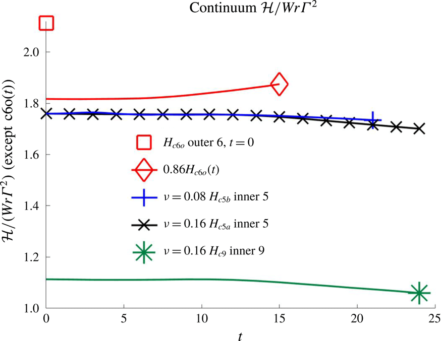
Continuum helicities normalised by
 $Wr\unicode[STIX]{x1D6E4}^{2}$
for two rings with one coiled. For inner rings with
 $m=5$
and 9 coils,
 ${\mathcal{H}}(0)\approx (1.8~\text{and}~1.1)Wr\unicode[STIX]{x1D6E4}^{2}$
until
 $t\approx 12$
, twice the reconnection time of
 $t\approx 7.5$
indicated by jumps in the topological numbers in figure 2(b). For an outer ring with six coils,
 $Wr\approx 0.16$
is small with
 ${\mathcal{H}}(0)\approx 2.1Wr\unicode[STIX]{x1D6E4}^{2}$
until reconnection ends, then
 ${\mathcal{H}}$
grows.
 $\unicode[STIX]{x1D6E4}=1720,\unicode[STIX]{x1D6E4}^{2}=3\times 10^{6}$
.

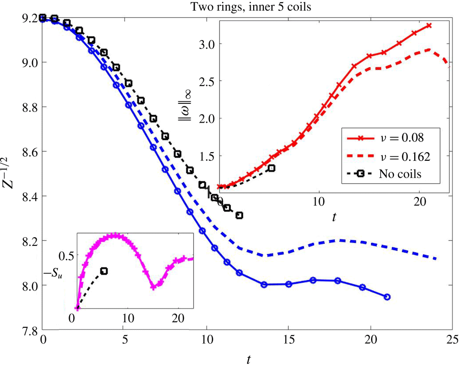
As the enstrophy
 $Z$
grows,
 $Z^{-1/2}$
decreases linearly for cases c5a and c5b until
 $t\approx 11$
, when reconnection finishes (when
 ${\mathcal{L}}_{S}$
rebounds in figure 2
b) and helicity starts changing. Cases c6o and c9 have similar
 $Z(t)^{-1/2}$
. The enstrophy growth is weaker for s
 $_{6}$
, a single ring with coils (not shown), and c0, nested rings with no coils, In the upper inset,
 $\Vert \unicode[STIX]{x1D714}\Vert _{\infty }$
has similar case-dependent growth. In the lower inset, the normalised enstrophy production
 $-S_{u}$
(2.3) is large for the 5-coil cases, independent of
 $\unicode[STIX]{x1D708}$
, and very weak for cases c0 (shown) and s
 $_{6}$
.

The following is observed for all the nested rings. Their global helicities
 ${\mathcal{H}}$
in figure 5 are preserved until at least
 $t=6$
and all have similar enstrophy growth, with the strongest for case c5b. For their topological numbers, the self-linking identity (1.1) is satisfied at all cases either by direct determination of
 $Wr$
,
 $Tw$
and
 ${\mathcal{L}}_{S}$
, or for case c9 by assuming that
 ${\mathcal{L}}_{S}=m=9$
. There are also almost no changes in these numbers until reconnection, including no exchange of
 ${\mathcal{L}}_{S}$
between the twist and the writhe.
Figure 2 shows how the structure and topological numbers for case c5a evolve. In figure 2(a), the
 $t=0$
centreline vortices are at the top and the
 $t=7.5$
structures are at the bottom, with the beginning of reconnection represented by the magenta bulges on the previously outer ring that contain helicity that has been transferred from the inner to the outer ring during reconnection.
Figure 2(b) shows that the topological numbers on that inner, coiled ring are relatively static for
 $t\leqslant 7.5$
with
 ${\mathcal{L}}_{S}=m=5$
,
 $Tw\lesssim 5$
and the writhe
 $Wr\approx 0.44$
. While twist does not become writhe, as reported experimentally (Scheeler et al.
Reference Scheeler, van Rees, Kedia, Kleckner and Irvine2017, figure 3), their
 $\unicode[STIX]{x1D70F}(s)$
profiles do deform, with the
 $\unicode[STIX]{x1D70F}(s)$
peaks splitting, beginning with those shown at
 $t=3$
in figure 3. Post-reconnection, some of the original inner coil, self-linking re-emerges at
 $t\geqslant 10.5$
with different topological numbers. There is a reduction of
 ${\mathcal{L}}_{S,in}$
on the original coiled ring, along with new, self-linking of
 ${\mathcal{L}}_{S,out}=1$
on the original outer ring from the
 $t=7.5$
magenta bulges. The net change in the global linking is
 $\unicode[STIX]{x0394}{\mathcal{L}}_{T}\approx -1$
(or using (1.2),
 $\unicode[STIX]{x0394}{\mathcal{H}}_{T}\approx -\unicode[STIX]{x1D6E4}^{2}$
).
The dashes in figures 2(a) and 4(a) show the azimuthal+vertical motion of the coils – motion that could be compared to experimental measurements. Quantitatively,
 $$\begin{eqnarray}\boldsymbol{u}_{in}=\overset{\boldsymbol{\cdot }}{\boldsymbol{x}}_{in}(s,t)=(u_{\unicode[STIX]{x1D719}\text{-}in}\hat{\boldsymbol{e}}_{\unicode[STIX]{x1D719}},u_{z\text{-}in})\quad \text{and}\quad \boldsymbol{u}_{out}=\overset{\boldsymbol{\cdot }}{\boldsymbol{x}}_{out}(s,t)=(u_{\unicode[STIX]{x1D719}\text{-}out}\hat{\boldsymbol{e}}_{\unicode[STIX]{x1D719}},u_{z\text{-}out}).\end{eqnarray}$$
The two
 $t=3$
components of
 $\boldsymbol{u}_{\bot }=\boldsymbol{u}-u_{\unicode[STIX]{x1D714}}\boldsymbol{T}$
, first averaged over the c5 inner ring, then for
 $U_{z}$
averaged over both rings, are
 $$\begin{eqnarray}\overline{u}_{z\text{-}in}=10.9,\quad \overline{u}_{\unicode[STIX]{x1D719}\text{-}in}\approx \overline{(u_{\bot }-\overline{u}_{z\text{-}in})}=10.3\quad \text{and}\quad U_{z}=0.5(\overline{u_{z\text{-}in}}+\overline{u_{z\text{-}out}})=6.8,\end{eqnarray}$$
consistent with the (2.9) prediction. The experimental case c9 has similar values, except with more coils its
 $\overline{u}_{\unicode[STIX]{x1D719}}$
is larger.
Using these velocities, figure 3 includes
 $s$
-profiles at
 $t=3$
of
 $u_{\unicode[STIX]{x1D714}}/\unicode[STIX]{x1D6E4}$
,
 $u_{\bot }/\unicode[STIX]{x1D6E4}$
and
 $W\!r_{s}=\unicode[STIX]{x2202}W\!r/\unicode[STIX]{x2202}s$
in order to obtain insights into the relationship between
 $Wr_{s}$
and
 ${\mathcal{H}}_{c}$
(2.14), an integral of
 $u_{\unicode[STIX]{x1D714}}$
, in the simulations and why the
 ${\mathcal{H}}_{c}$
from the Scheeler et al. (Reference Scheeler, van Rees, Kedia, Kleckner and Irvine2017) experiments are unexpectedly small. These insights are as follows.
First, consider the small
 $t=0$
values of
 $Wr$
and
 ${\mathcal{H}}_{c}$
in table 1, with
 ${\mathcal{H}}_{c}/\unicode[STIX]{x1D6E4}^{2}\sim 0.15Tw$
, which is significantly less than the (1.2) prediction that
 ${\mathcal{H}}_{T}/\unicode[STIX]{x1D6E4}^{2}\sim {\mathcal{L}}_{S}\sim Tw$
. Second,
 $u_{\unicode[STIX]{x1D714}}$
has extensive negative excursions,
 $u_{\unicode[STIX]{x1D714}}\lesssim 0$
. These negative excursions and small averages could make their line integral,
 ${\mathcal{H}}_{c}$
, difficult to determine experimentally given their acknowledged difficulties in measuring the centreline velocities and could explain why their
 $t=0$
experimental helicities, their total
 ${\mathcal{H}}_{s}$
, are consistently the order of one-third of
 $Wr\unicode[STIX]{x1D6E4}^{2}$
, compared to the equivalent simulations: cases s
 $_{6}$
, c6o and c9. Could this be due to a consistent
 $\unicode[STIX]{x03C0}^{-1}$
bug in their analysis? Or can this effect be reproduced in the simulations?
Surprisingly, it seems likely that the two stages in the analysis of case c9 could be reproducing this effect. In the first stage, when every point on the trajectory was used to calculate the topological numbers, besides the difficulties noted in table 1 with
 ${\mathcal{L}}_{S}$
for c9, the c9 writhe was
 $Wr_{1}\approx 0.85$
, such that
 $Tw_{1}+Wr_{1}\approx 8.4<m=9$
and
 ${\mathcal{H}}_{c}$
was approximately half the global helicity
 ${\mathcal{H}}$
. However, with the fourth-point algorithm, for the values in table 1,
 $Tw_{4}+Wr_{4}\approx 9=m$
. Since it is writhe more than twist that is tied to
 ${\mathcal{H}}_{c}$
(2.14), this could be an example of how large fluctuations in the centreline velocities could lead to underestimates of
 ${\mathcal{H}}_{c}$
.
3.3 Two rings, outer coiled
Figure 4 gives the structures and topological numbers of case c6o, with six coils on the outer ring. Before
 $t=10.5$
, on the coiled ring
 ${\mathcal{L}}_{S}=m=6$
,
 $Tw\lesssim 6$
and the writhe is small,
 $Wr\approx 0.16$
. At
 $t=11.25$
,
 ${\mathcal{L}}_{S}$
and
 $Tw$
jump to approximately 0, then briefly rebound to approximately
 ${\mathcal{L}}_{S}=6\gtrsim Tw$
for
 $t\geqslant 13.5$
, before the rings merge at
 $t\approx 15$
. Throughout the calculation, the global
 $\Vert \unicode[STIX]{x1D714}\Vert _{\infty }$
stays on the black vortex line running through the inner, uncoiled ring, plateauing at
 $\Vert \unicode[STIX]{x1D714}\Vert _{\infty }\approx 2$
at
 $t\approx 10.5$
, smaller than for case c5, while the local
 $\max |\unicode[STIX]{x1D714}|$
on the outer coiled ring barely changes.
3.4 Time dependencies of global
 ${\mathcal{H}}$
and vorticity statistics

The evolution of the continuum helicity
 ${\mathcal{H}}$
(2.14) and the enstrophy
 $Z$
(2.3) given in figures 5 and 6 allows comparisons to be made between the reconnecting coiled rings and the reconnection of trefoil vortex knots and anti-parallel vortices in Kerr (Reference Kerr2018a
,Reference Kerr
b
).
First the similarities between the two-ring configurations are examined. By weighting
 ${\mathcal{H}}$
by
 $Wr\unicode[STIX]{x1D6E4}^{2}$
, figure 5 shows that
 ${\mathcal{H}}\sim (1\text{ to }2)Wr\unicode[STIX]{x1D6E4}^{2}$
until there is reconnection, already indicated by the sudden changes in
 $Tw$
and
 ${\mathcal{L}}_{S}$
in figures 2(b) and 4(b) for
 $t\sim 7.5$
and 10.5, respectively. One difference between the inner and outer coiled ring cases is that post-reconnection,
 ${\mathcal{H}}/Wr\unicode[STIX]{x1D6E4}^{2}$
decreases for the inner coiled cases (c5a, c5b, c9) and increases for the outer coiled case (c6o). For the trefoils, reconnection is also associated with when
 ${\mathcal{H}}$
begins to change (Kerr Reference Kerr2018a
).
For the enstrophy
 $Z$
, as it grows,
 $Z^{-1/2}$
decreases linearly for all the nested, coiled cases during the first temporal stage, defined by relatively constant
 ${\mathcal{H}}$
up to
 $t\approx 7.5$
to
 ${\approx}11$
, depending on the case. This scaling improves slightly between cases c5a and c5b as
 $\unicode[STIX]{x1D708}$
decreases. If there are no coils, case c0, enstrophy growth comes only from the two-ring leapfrog interaction and if there is only one multicoil ring, case s
 $_{6}$
, from the relaxation of the coils, suggesting that the linear in time
 $Z^{-1/2}$
scaling requires both coils and nesting.
Is the
 $Z^{-1/2}$
scaling for nested coiled rings viscous or inviscid? Consider the insets in figure 6, with
 $\Vert \unicode[STIX]{x1D714}\Vert _{\infty }$
, the maximum of vorticity, in the upper right and
 $-S_{u}=C\unicode[STIX]{x1D74E}\unicode[STIX]{x1D64E}\unicode[STIX]{x1D74E}/Z^{3/2}$
, the normalised enstrophy production (2.3) or velocity-derivative skewness, in the lower left. Both are independent of
 $\unicode[STIX]{x1D708}$
until approximately
 $t=6$
, implying that the calculations are essential inviscid, or Euler, until then. Given that, then the enstrophy growth can be understood in terms of the variations in
 $-S_{u}$
. As
 $-S_{u}$
is increasing strongly for
 $t\leqslant 3$
,
 $Z$
does not change significantly. Then as the inner ring is pulled outside of the outer ring,
 $-S_{u}$
is relatively constant, allowing use of the classic closure of
 $\text{d}Z/\text{d}t=C_{Z}|S_{u}|Z^{3/2}$
, which gives the observed linear
 $Z(t)^{-1/2}$
scaling.
Longer regimes of linearly decreasing
 $Z^{-1/2}$
scaling were previously found during the reconnection of both trefoils (Kerr Reference Kerr2018a
) and anti-parallel vortices (Kerr Reference Kerr2018b
), with two significant differences. First, their initial configurations do not have coils; second, it is
 $B_{\unicode[STIX]{x1D708}}(t)=(\sqrt{\unicode[STIX]{x1D708}}Z)^{-1/2}$
that converges, not simply
 $Z^{-1/2}$
. What might be similar is that the
 $(\sqrt{\unicode[STIX]{x1D708}}Z)^{-1/2}$
scaling does not begin until viscous reconnection begins and some twist develops, determined crudely for the trefoils and seen visually on the reconnected anti-parallel vortices. Could this mean that linear
 $Z^{-1/2}$
regimes require vortices with twist? Either imposed or generated by viscous reconnection?
4 Summary
The three primary results of this paper are:
(1) A set of algorithms has been demonstrated that are able to independently extract the writhe
$Wr$
, the twist
$Tw$
and the self-linking
${\mathcal{L}}_{S}$
numbers of closed trajectories determined from grid-based vector fields. In addition to the Gauss linking algorithms (2.13) for
$Wr$
and
${\mathcal{L}}_{S}$
(Kerr Reference Kerr2018a
), by taking every fourth point on trajectories
$\boldsymbol{x}_{j}(s)$
(2.10), the Frenet–Serret (2.11) twist (2.12) can now be found.(i) Furthermore, since the experiments are already finding digital trajectories, these direct methods for calculating the topological numbers might be capable of replacing the use of the trajectory crossings (Scheeler et al. Reference Scheeler, Kleckner, Proment, Kindlmann and Irvine2014), with validation provided by
${\mathcal{L}}_{S}=Tw+Wr$
(1.1).(ii) The current limitations of using these methods for quantitative analysis, in particular for tightly coiled vortices, are discussed. However, even then, and as configurations become turbulent (Kerr Reference Kerr2018a ), they can provide useful qualitative insights.
(2) For the Scheeler et al. (Reference Scheeler, van Rees, Kedia, Kleckner and Irvine2017) coiled ring experiments, only their
$t=0$
writhe
$Wr$
values are confirmed, and by applying the twist integral (2.12) to the coil trajectories (2.7) one gets
$Tw\gg Wr$
, not
$Tw\ll Wr$
.(i) Their self-linking
${\mathcal{L}}_{S}$
numbers obtained by using
${\mathcal{H}}_{c}$
(2.14) for
${\mathcal{H}}_{T}$
in (1.2) are also inconsistent with values obtained from using the analytic centreline trajectories (2.7).(ii) The origin of the faulty
${\mathcal{L}}_{S}$
values is probably twofold. First, it is empirically shown that for single coils with a large twist
$Tw$
that
${\mathcal{H}}_{c}\sim Wr\unicode[STIX]{x1D6E4}^{2}$
(1.3) with
$Wr\ll {\mathcal{L}}_{S}$
. Not
${\mathcal{H}}_{c}\sim {\mathcal{L}}_{S}\unicode[STIX]{x1D6E4}^{2}$
(1.2). Second, there could be errors related to
$u_{\unicode[STIX]{x1D714}}<0$
in (2.14), as discussed in § 3.3.
(3) Consistent with the numerical results for reconnecting trefoil vortices and anti-parallel vortices, until the first reconnection is finished, the global helicity
${\mathcal{H}}$
is preserved and there is linear
$Z^{-1/2}(t)$
enstrophy scaling. Comparison of the configurations suggests that twist, either imposed or due to viscous reconnection, could be the common property.


These final results confirm that there is a relationship between the evolution of the topological and the continuum dynamics, with the writhe and twist playing complementary roles, but not as suggested by Scheeler et al. (Reference Scheeler, van Rees, Kedia, Kleckner and Irvine2017). Besides continued analysis of the existing coiled rings, more coiled ring calculations are needed. These should include rings with thinner vortices and a wider range of viscosities. Furthermore, with the new tool for finding the twist and better insights into its role, the trefoil calculations need to be revisited.
Acknowledgements
I wish to thank S. Schleimer and M. A. Berger for discussions on topological structures. Computing resources have been provided by the Centre for Scientific Computing at the University of Warwick.