INTRODUCTION
The common or brown shrimp Crangon crangon L. is an abundant epibenthic crustacean over its entire Atlantic coastal range from Norway to Morocco and throughout the Mediterranean and Black Seas. It especially favours shallow coastal and estuarine waters with sandy or muddy bottoms (Tiews, Reference Tiews1970). Because of its generally high abundance, the species plays an important functional role in coastal ecosystems as prey species for fish, crustaceans and birds (Pihl, Reference Pihl1985; Henderson et al., Reference Henderson, James and Holmes1992; Del Norte-Campos & Temming, Reference Del Norte-Campos and Temming1994; Walter & Becker, Reference Walter and Becker1997) and as predator on juvenile stages of epi- and infauna (Pihl & Rosenberg, Reference Pihl and Rosenberg1984; Van der Veer et al., Reference Van der Veer, Bergman, Dapper and Witte1991, Reference Van der Veer, Feller, Weber and Witte1998; Ansell & Gibson, Reference Ansell and Gibson1993; Oh et al., Reference Oh, Hartnoll and Nash2001; Amara & Paul, Reference Amara and Paul2003). Its general biology is well known (Tiews, Reference Tiews1970) and indicates geographical variability in the species life history. However, at present, no detailed information is available as to the extent to which this variability is caused by either genotypic and/or phenotypic plasticity in order to adapt to different environmental conditions.
Besides a key ecological role in shallow water ecosystems, brown shrimp is commercially exploited, especially in the North Sea. As for other fishery resources, successful stock management requires knowledge of the population structure (Cadrin, Reference Cadrin2000). Tools applied so far to investigate C. crangon's population structure were the variability in morphometric characters (Maucher, Reference Maucher1961; Henderson et al., Reference Henderson, Seaby and Marsh1990; Beaumont & Croucher, Reference Beaumont and Croucher2006) and investigations on allozymes (Abdullah & Shukor, Reference Abdullah and Shukor1993; Bulnheim & Schwenzer, Reference Bulnheim and Schwenzer1993; Beaumont & Croucher, Reference Beaumont and Croucher2006) and on AFLP (amplified fragment length polymorphism) locus (Beaumont & Croucher, Reference Beaumont and Croucher2006). All these studies were performed on a small scale (100 km), with the exception of Bulnheim & Schwenzer (Reference Bulnheim and Schwenzer1993). These authors were able to identify on a large scale (1000 km) four regional groups: (1) the North Sea and Baltic Sea; (2) the North Atlantic Ocean; (3) Portugal; and (4) the Adriatic Sea. While Abdullah & Shukor (Reference Abdullah and Shukor1993) found little genetic difference between two populations in the south of Wales, Beaumont & Croucher (Reference Beaumont and Croucher2006) detected a population subdivision between east and west coast in the UK, both by allozyme and AFLP variation. Two morphometric studies even suggested the existence of a much more detailed population structure on a smaller scale. Maucher (Reference Maucher1961) suggested differences between North Sea and Baltic Sea populations and Henderson et al. (Reference Henderson, Seaby and Marsh1990) distinguished already six subpopulations around British waters. However, in a third more recent study (Beaumont & Croucher, Reference Beaumont and Croucher2006) from five sites around the UK only one was distinctively identified morphologically from the others, by possessing longer telsons and inner uropods. Nevertheless, all these conclusions on spatial variability were drawn from single sampling programmes on limited temporal extent.
To date, the studies by Maucher (Reference Maucher1961) and Henderson et al. (Reference Henderson, Seaby and Marsh1990) have never been expanded despite their promising results (high resolution). In this study, we applied the method of variability in morphometric characters to analyse the subpopulation structure of brown shrimp C. crangon over its entire distributional range from Norway until the Black Sea including the Mediterranean Sea, especially in what concerns its scale resolution at a larger scale (1000 km). In addition to this single sampling programme, at four stations monthly sampling was used to study temporal variability.
MATERIALS AND METHODS
Data collection
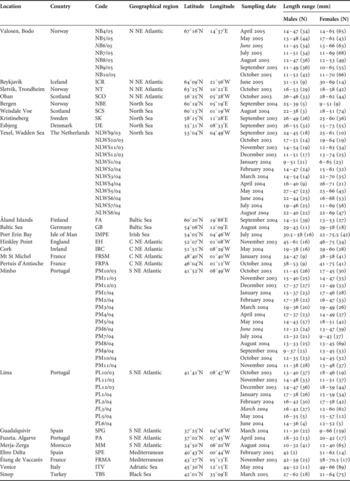
Samples were collected by beam-trawl or push-net at intertidal stations distributed over the whole geographical range of distribution of the species (Figure 1). Table 1 presents a list of sampling locations, their GPS positions, date of sampling, number and length-range of analysed shrimps by sex. All shrimps were checked individually for species identification according to Smaldon (Reference Smaldon1979). Since sampling took place in different time periods, potential bias by temporal variability was also checked at four different locations spread over the distributional range: (1) Valosen estuary (Bodo, Norway); (2) Texel (Dutch Wadden Sea, The Netherlands); (3 and 4) Minho and Lima estuaries (north of Portugal). At these locations, shrimps of different size and sex were collected and measured monthly (Table 1).
Sample locations for Crangon crangon and corresponding geographical regions. Sample codes correspond to those in Table 1.

Sampling information of Crangon crangon: location, code, geographical region, GPS positions, sampling date and length-range and sample size (N) per sex. Samples chosen for local scale spatial variability analysis in italic. Sampling sites are also indicated on the map in Figure 1.

Data analysis
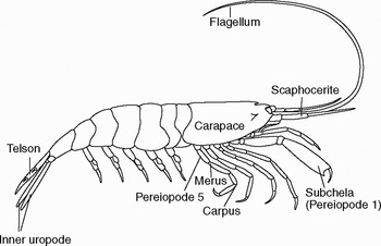
From each sample, several shrimps (Table 1), when possible regularly divided over sex and total size-range (defined as the total length (TL), the distance between the end of folded uropods/telson and the tip of scaphocerites) (Schockaert, Reference Schockaert1968; Schumacher & Tiews, Reference Schumacher and Tiews1979), were examined for nine characters (Figure 2), following Henderson et al. (Reference Henderson, Seaby and Marsh1990): carapace length (CAR); telson length (TEL); inner uropod length (INNLE); maximum inner uropod width (INNWI); maximum sub-chelae length (SUBCLE); maximum sub-chelae width (SUBCWI); length of segment 4 (merus) of the first pereiopod (PERI); maximum length of segment 4 (merus) of pereiopod 5 (MAX4); maximum length of segment 5 (carpus) of periopod 5 (MAX5). Sex was determined as described by Tiews (Reference Tiews1970): (1) measuring the length of the 2nd outer and inner antennules; and (2) observing endopodites' morphology on the 1st (bigger and spoon-like in females) and 2nd pleopods (biramous in males). All measurements were performed to the nearest 0.001 mm total length on a computer screen from digital images from a binocular by means of Axio Vision 4.1 software or with Leica Qwin 500 software. Animals with regenerated appendages or missing some of the measured parts of the body were rejected.
Morphometric variables measured on Crangon crangon specimens.

Statistical analysis
Isometric growth was tested by determining the correlation between each morphometric variable and TL for each sex per location and sampling date using Pearson correlation coefficient and Bonferonni probability. Generalized linear models (GLM) (without constant) were applied to investigate linear relationships between the morphometric parameters (dependent variables) and TL (independent variable), per location and per sampling month for each sex, with location and date of sampling considered independent variables and defined as categories. No constant was used in GLM because at zero mm TL, all variables were assumed to be also zero in size.
Since most variables for each sex were normally distributed in each location and in each sampling date in the four main locations (Bodo, Texel, Minho and Lima) (Shapiro–Wilk test, 0.05 < P < 0.000), no transformation was performed. All morphometric variables were corrected for size by dividing each measurement by respective TL, which transformed the variables into the same order of magnitude and hence there was no need to normalize them.
To check for similarities between sexes, locations/regions and dates of sampling an analysis of similarities (ANOSIM) was applied to the morphometric measurements corrected for TL, using Euclidian distance because it can measure distances between any two points in space (Clarke & Warwick, Reference Clarke and Warwick2001). ANOSIM is a permutation test analogue of the standard ANOVA (analysis of variance), used to detect differences among groups, which calculates the probability of random occurrence of the observed groups. In ANOSIM the test statistic R is a comparative measure of the degree of separation of sites based on rank similarities between samples. Usually it falls between zero and one indicating some degree of discrimination between sites, which may be significant or not. Larger values are indicative of complete separation and values close to zero represent no differences between sites. However, when there are many replicates at each site R may be very small and yet significantly different from zero (Clarke & Warwick, Reference Clarke and Warwick2001).
Multivariate principal components analysis (PCA) was used to detect variation between the nine morphometric variables and among locations/regions. Additionally another multivariate technique, a linear discriminant analysis was performed to determine our ability to distinguish between locations/regions.
Sexual and temporal variability was evaluated per sampling date in the four main locations. Only mature individuals between 40 to 50 mm TL were used in sexual variability analysis to avoid possible morphological differences associated to size-class. However, due to low numbers of females of 40–50 mm TL in samples from other sites and after proving isometry, all mature females 40–60 mm TL were used in temporal and spatial variability analysis. Spatial variability was evaluated at two scales of resolution: large scale comparing samples collected in various locations pooled per main geographical region and local scale comparing samples from all locations, with only one sample chosen randomly from the four main sites (Table 1).
Pearson correlation, GLM and linear discriminant analysis were performed in Systat 11.0. PCA and ANOSIM analyses were performed with Primer 6 software (PRIMER-E, Plymouth Marine Laboratory, UK).
RESULTS
General results: isometry and sexual variability
Morphometric variables were positively correlated with TL for both sexes (0.42 < Pearson correlation coefficient < 0.99; P < 0.001), with some exceptions due to insufficient data, suggesting linear relationships, which was confirmed by the GLM analysis (Table 2). Therefore there was no evidence of allometric growth for both females and males for the size-range used in this study and hence no data transformation was performed.
Maximum, minimum and average regression coefficients obtained by generalized linear model for each morphometric variable per sex of Crangon crangon. Abbreviations for variables in the text.

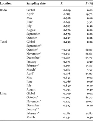
Except for Minho estuary where only three males 40–50 mm were caught and hence differences between sexes were not possible to analyse, ANOSIM global tests for sexual variability resulted in a significant difference (P < 1%) but at a low value of R (R < 0.300) (Table 3). Although this could suggest that overall both sexes were not distinguishable, when analysing each sampling date in the pairwise tests (Table 3) significant sexual variability (P < 5%) was observed in several months. Moreover in some of these cases (August and September in Bodo; January and May to August in Texel) R statistic was close to 1 (R > 0.650) indicating that individuals of the same sex were more similar to each other than between sexes.
Results of ANOSIM analysis (R-statistic and significance level) between sexes of Crangon crangon: global and pairwise tests for each sampling date. Significant values shown in bold; *non-significant values; **insufficient data (only one sex present in the sample).

Spatial variability: large versus local scale resolution
At the large scale, despite the low value of R, considering the enormous amount of information, the variability between main geographical regions (North, central and south north-eastern Atlantic, North, Irish, Baltic, Mediterranean, Adriatic and Black Seas) was significant (R = 0.291; P = 0.02%) (Table 4). In the pairwise tests the Adriatic and Black Seas and north north-eastern Atlantic were significantly different from all other areas (R > 0.160; P < 5%). The Mediterranean Sea differed significantly from all regions except for the North Sea and central north-eastern Atlantic (R = 0.130; P = 6.10% and R =−0.036; P = 63.5%, respectively). Yet within the Atlantic area, shrimps from several regions were statistically indistinguishable: the North Sea was similar to the Baltic and Irish Seas; further, the Baltic was similar to the Irish Sea and the central and southern north-eastern Atlantic; and the central north-eastern Atlantic was also similar to the Irish Sea. At the local scale, comparing morphometrics between each of the 25 locations, the huge amount of data made interpretation very difficult and, although there was significant variability between locations (R = 0.447; P = 0.02%), no clear pattern could be generated from the results, since nearby locations could be distinguished from each other but were indistinguishable from distant sites.
Results of ANOSIM analysis of Crangon crangon: global and pairwise tests between each geographical region. R-statistic below diagonal and significance level (%) above diagonal. Significant values shown in bold.

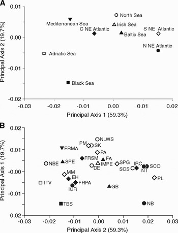
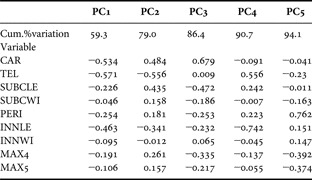
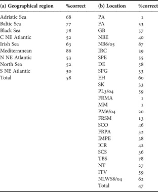
Because of the huge amount of data only the PCA centroids (PCA scores' average) per geographical region and per location are shown in a two-dimensional plot (Figure 3). The first two PCA axes explained 79% of total variance (Table 5). Negative loadings for PC1 were produced in all variables, with telson and carapace allometric coefficients presenting a stronger influence (−0.571 and −0.534, respectively). While 2-D PCA centroids plot per location were not obvious in respect to the subpopulation structure (Figure 3b), per geographical region the main subpopulations detected in ANOSIM (Adriatic, Black Sea, Mediterranean, north north-eastern, central and south north-eastern Atlantic) are clearly apart (Figure 3a). According to discriminant analysis results (Table 6) several locations had less than 40% of data assigned correctly to the location, while at larger scale individuals from the regions mentioned above were assigned correctly at more than 50%.
Two-dimensional PCA centroids (scores average for the first two principal axes) plot performed on the morphometric variables of all Crangon crangon females 40 to 60 mm (a) from each geographical region and (b) from each location. Location codes in Table 1.

Cumulative percentage of variation explained by the first five principal components from the PCA performed on the morphometric variables of all Crangon crangon females 40 to 60 mm and respective eigenvectors. Abbreviations of variables given in the text.

Percentage of individuals of Crangon crangon correctively assigned to its original group: (a) geographical region and (b) location, according to discriminant analysis. Location codes in Table 1.

Temporal variability
Temporal variability was observed in three of the four main locations. ANOSIM global tests showed a significant level for temporal variability (P < 5%), except for Bodo due to the extremely low value of R (R = 0.052; P = 0.06%). Despite the low value of R for Minho (R = 0.261; P = 0.02%) and Lima (R = 0.114; P = 0.50%), due to the large number of samples, the difference between sampling dates can still be considered significant. Whilst for Texel the mid-range value of R (R = 0.323; P = 0.02%) indicated significant differences between sampling dates. Furthermore, the pairwise tests of ANOSIM analysis revealed several significantly different pairs of sampling dates by both their significance level (P < 5%) and their mid-range (0.300 < R < 0.650) to high value of R (R > 0.650).
DISCUSSION
Population structure of a species is usually referring to its genetic background, the members of an independent subpopulation sharing a common pool of genetic characteristics and being to some extent isolated from other populations. Crangon crangon's population genetic structure has been studied previously using molecular tools (DNA sequencing). It was found strong population structuring with four major phylogeographical groups: the north-east Atlantic, the western Mediterranean, the Adriatic Sea and the Black Sea (Luttikhuizen et al., Reference Luttikhuizen, Campos, Bleijswijk, Peijnenburg and van der Veer2008). A similar pattern might then be expected using morphometric tools. At a local scale, Abdullah & Shukor (Reference Abdullah and Shukor1993) identified variation at several allozyme loci but with little genetic difference between two locations in the south of Wales, while Bulnheim & Schwenzer (Reference Bulnheim and Schwenzer1993) found some differentiation in the north-eastern Atlantic based on three polymorphic allozyme loci. Beaumont & Croucher (Reference Beaumont and Croucher2006) detected higher levels of polymorphism in two allozyme loci suggesting a population subdivision between the east and west coast in the UK, further confirmed by the analysis of three AFLP loci. Weetman et al. (Reference Weetman, Ruggiero, Mariani, Shaw, Lawler and Hauser2007) using AFLP drew the same conclusion of some Atlantic population differentiation among locations from around the British Isles and from the Baltic Sea. Based on these studies broad-scale homogeneity of fishery stocks should not be assumed.
Phenotypic plasticity can also be expressed within a subpopulation. Both genetic and phenotypic characters can be reflected in shape and biometry of a subpopulation, two components of morphology which are expected to contain information about a biological group reflecting evolutionary processes responsible for diversity (Hammer, Reference Hammer2002). Therefore morphometric analysis can be used to study patterns of geographical variation and differences among ‘populations’ intended to define subpopulation structure as discriminate ‘phenotypic stocks’ (Cadrin, Reference Cadrin2000), which is particularly important for fisheries management. In the present study we considered that each subpopulation would be defined by significant differences in a set of morphometric parameters. The question remains as to which morphological features will best explain the relationships, since the choice of descriptors can greatly affect the conclusions (Strauss, Reference Strauss2001). One way to avoid possible bias is to measure as many variables as possible in a multivariate approach (Cadrin, Reference Cadrin2000).
We have measured the same nine morphometric parameters used by Henderson et al. (Reference Henderson, Seaby and Marsh1990). Data were then analysed differently, because allometric growth was assumed in their work. We tested and confirmed isometry between morphological parameters and total length, as Beaumont & Croucher (Reference Beaumont and Croucher2006) did with a similar dataset but from five locations around the UK, and hence data transformation would not change the observed trends. Only size standardization of the data was necessary to reduce it to the same order of magnitude and that was done by simply dividing each parameter by total length. Moreover, besides an ordination method we used an analysis of similarities (ANOSIM) and discriminant analysis to detect differences among groups, and hence strengthening the trends' reliability.
The conclusions of our study are in part similar to Henderson et al. (Reference Henderson, Seaby and Marsh1990), since at local scale we can distinguish almost as many ‘subpopulations’ as the number of sampled locations. However, despite that environmental conditions such as temperature, salinity and food availability affect body development and hence body morphology, it does not seem reasonable that each location corresponds to a different population defined by a particular morphotype. Given the mobility of C. crangon at the planktonic larval stage, when studying spatial variability at a large scale, grouping samples by main geographical region—north, central and south north-eastern Atlantic, North, Irish, Baltic, Mediterranean, Adriatic and Black Seas—allowed the analysis of larger subpopulation structures, with Adriatic and Black Sea populations very clearly recognizable. Remarkably, some Atlantic regions (central north-eastern Atlantic, North, Irish and Baltic Seas) were morphometrically homogeneous, which suggests that the observed significant differences at local scale may actually be caused by high individual variability within a single population. Although the Mediterranean could be distinguished from most regions, including the neighbouring south north-estern Atlantic region, it was not distinguishable from the central north-eastern Atlantic and North Sea, possibly suggesting a clinal variation in the morphometric variables chosen, i.e. a gradual change in those features with no clear division reflecting geographical regions. Therefore, those widely distant populations (Mediterranean Sea and central north-eastern Atlantic and North Sea) seem to be similar considering only the nine morphological variables analysed, requiring the study of more variables to be more sensitive.
Within the Mediterranean, Adriatic and Black Seas, the homogeneous pattern observed in the central part of the vast Atlantic region would not be expected because the continental shelf is non-continuous over these three regions. In contrast, the shelf is continuous along the European Atlantic coast. However, the variability of some locations within the Atlantic suggests the existence of discontinuity boundaries between subpopulations (neighbour locations from different subpopulations where morphometric variability is higher). This could be the case of several sites in the North Sea—Bergen and Kristineberg in relation to north north-eastern Atlantic; Esbjerg in relation to central north-eastern Atlantic and to Baltic Sea; and Texel in relation to central north-eastern Atlantic; GB in the Baltic in relation to the North Sea and Minho in south north-eastern Atlantic in relation to central north-eastern Atlantic. However, the sampling programme was not designed with this perspective in mind and hence several locations should be analysed further to be conclusive. Furthermore, the separation between south north-eastern Atlantic and the Mediterranean populations would require the morphometric analysis of a very relevant site between the Strait of Gibraltar and the Oran–Almeria Front, both already described as possible barriers between populations of marine species (Patarnello et al., Reference Patarnello, Volckaert and Castilho2007).
Morphometrics' resolution failed at local scale possibly due to the huge variability within locations. Brown shrimp dispersal potential is not easy to assess. Epibenthic adults and eggs, which are not free floating but carried by females, are not expected to be much influenced by currents; but the pelagic larval stage which lasts for 5 to 10 weeks according to temperature (Criales & Anger, Reference Criales and Anger1986), may be more susceptible to passive transport. Also, seasonal migrations may be expected to contribute to species dispersal. Temporal variability had not been studied in those two previous works where only one dataset was analysed per location. We followed monthly the morphometrics at four local populations and detected variability between sampling dates, which might be related partly to seasonal migrations: Atlantic brown shrimp, especially males, are known to migrate into deeper areas when temperature cools down, returning to shallow waters in spring/summer (Lloyd & Yonge, Reference Lloyd and Yonge1947; Henderson & Holmes, Reference Henderson and Holmes1987; Beukema, Reference Beukema1992; Attrill & Thomas, Reference Attrill and Thomas1996; Drake et al., Reference Drake, Arias, Baldó, Cuesta, Rodriguez, Silva-Garcia, Sobrino, Garcia-Gonzalez and Fernandez-Delgado2002; Gibson et al., Reference Gibson, Robb, Wennhage and Burrows2002). The inverse migration pattern is observed in the Mediterranean (Labat, Reference Labat1977). Sampling in different periods may then provide different morphometric information because available individuals may not include the entire population pool. Moreover food availability and predation pressure might also vary seasonally affecting the morphometry of the population. Finally, the fact that the brown shrimp's reproduction takes place during a long period with different cohorts experiencing diverse environmental conditions for development and growth may also contribute to morphometrics' temporal variation and irreversible non-genetic adaptation (Kinne, Reference Kinne1962; Van der Veer et al., Reference Van der Veer, Bies and Witte2000). This might affect its physiological performance and hence growth and perhaps result in spatial morphometic variability. For example, populations in the Bristol Channel reproduce twice per year, in late winter and early summer. It is possible that individuals from each of these cohorts, which experience widely differing temperatures during early development, may differ appreciably in their morphometrics. In conclusion, conventional morphometrics is capable of resolving large-scale brown shrimp subpopulation structure and indicates the existence of Adriatic, Black Sea, Mediterranean and Atlantic populations. But it is not useful at a small scale because of large between individual and temporal variabilities. This variability might be related to two particular features of the life cycle, seasonal migrations and the long reproductive period.
ACKNOWLEDGEMENTS
The authors would like to thank all who provided samples, namely Alain Crivelli, Audrey Geffen, Bernd Mieske, Bjorn Gunnarsson, Davide Tagliapietra, Erdogan Cicek, Hamid Taleb, Jarle Mork, John Davenport, Josianne Strottrup, Katri Aanio, Leif Pihl, Margarida Cristo, Peter Henderson, Pilar Drake, Richard Nash, Robin Gibson, Sabri Bilgin, Suzane Henderson and Yves Desauney, and those who helped in sampling, namely José Carlos Antunes, Eduardo Martins, Luis Scott, Sascha Sjollema, Sofia Tavares, Sónia Mendes, Stig Skreslet and Vânia Freitas. We are also grateful to Mathieu Cusson, Peter Henderson, Ana Bio and Eric Meesters for statistical advice and support and to Gonçalo Dumas and Sérgia Dias for providing the figures. This study was funded by FCT, Portugal, through the grant SFRH/BD/11321/2002 and the project POCI/CLI/61605/2004.