2. Effect of magnetic perturbations

The transport of electrons in enclosed stochastic magnetic fields is usually described with the Rechester–Rosenbluth diffusion coefficient $D_{RR}={\rm\pi}qv_{\Vert }R({\it\delta}B/B)^{2}$ (Rechester and Rosenbluth Reference Rechester and Rosenbluth1978). Here, $q$ is the safety factor, $v_{\Vert }\simeq c$ is the parallel velocity, $R$ is the major radius and ${\it\delta}B/B\equiv \sqrt{\langle ({\it\delta}B/B)^{2}\rangle _{{\it\psi}}}$ is the flux-surface-averaged normalized magnetic perturbation amplitude as a function of radius. In mixed magnetic topologies consisting of magnetic islands, intact toroidal magnetic surfaces and stochastic regions, this diffusion coefficient is not valid (Mynick and Strachan Reference Mynick and Strachan1981; Myra and Catto Reference Myra and Catto1992). In such circumstances, some fraction of the electrons will be trapped in magnetic islands, and the confinement time of these particles can equal the characteristic system evolution time. Furthermore, in open chaotic systems, such as the edge region of a magnetically confined plasma in the presence of external magnetic perturbations, not only is the Rechester–Rosenbluth diffusion not applicable, but the diffusive approach itself breaks down. Unlike in the case for enclosed stochastic fields, the region of increased transport (compared with the unperturbed case) extends all the way to the wall, making it easier for particles to get lost. As was confirmed by numerical simulations described in this paper, the runaway electron flux starting from a certain radial position is not proportional to the runaway density gradient, but to the local runaway density itself. If a flat runaway profile is initialized, losses occur immediately all around the simulation zone, i.e. the flux is not gradient-driven, as the inital density gradient is zero. This dynamics is due to the open ergodic region that is created by the Resonant Magnetic Perturbation (RMP) coils. It should be noted that the diffusive approach may still be applicable in closed ergodic regions. The net radial displacement of the particles is highly sensitive to the initial position and can differ by several orders of magnitude. Particles born within resonant loss regions will reach the outer edge of the plasma faster than the rest and be lost to the wall. Since the system is open at the plasma edge, there is no return flux of fast electrons, and hence the density gradient is not the governing factor in the evolution, as it would be in a diffusive picture. As we will show, this process can be approximated with a position-dependent exponential loss of particles, which describes the ensemble behaviour with reasonable accuracy.

In an axisymmetric tokamak equilibrium the magnetic topology consists of nested magnetic surfaces that provide good particle confinement. The main loss mechanism for fast electrons is due to the drift orbit shift associated with the energy gain (Papp et al. Reference Papp, Drevlak, Fülöp and Helander2011a ,Reference Papp, Drevlak, Fülöp, Helander and Pokol b ), which is determined by the electric field evolution. In the simulations presented here we use static externally imposed magnetic fluctuations on a static equilibrium field with nested toroidal magnetic surfaces. Whenever a magnetic perturbation is present, the topology of the magnetic field is strongly modified. There appear island chains (the locations of which are correlated with the low-order rational values of the rotational transform ), together with intact but deformed magnetic surfaces (KAM barriers Kolmogorov Reference Kolmogorov1957; Moser Reference Moser1962 and Arnold Reference Arnold1963) at irrational  values. In between these, ergodic zones are formed.

We solve the relativistic gyro-averaged equations of motion for test energetic electrons in a perturbed field with the ANTS code (Papp et al. Reference Papp, Drevlak, Fülöp and Helander2011a ). The simulations have been carried out for a specific ITER-like scenario as described in Papp et al. (Reference Papp, Drevlak, Fülöp, Helander and Pokol2011b ). The perturbations are externally imposed by $9\times 3$ quasi-rectangular perturbation coils at the low field side of the device. In the configuration we use (formerly labelled ‘B’ in Papp et al. Reference Papp, Drevlak, Fülöp, Helander and Pokol2011b ), electrical currents flowing in these coils generate a 120° rotationally symmetric perturbation field that decays radially towards the inside of the plasma and results in a relative perturbation strength ${\it\delta}B/B>O(10^{-3})$ outside the ${\it\psi}=0.5$ flux surface (the normalized radius relates to the normalized flux as $r/a\simeq \sqrt{{\it\psi}}$ , where $a$ is the minor radius of the torus).

To determine the evolution of the particle ensemble in such a topology, a direct calculation of test particle trajectories has been carried out. In each simulation a minimum of 40 000 test particles with 1 MeV energy were launched parallel to the magnetic field lines with various starting position distributions. In the simulations we use a time-dependent electric field obtained for an ITER-like disruption scenario calculated with a model of the coupled dynamics of the evolution of the radial profile of the current density (including the runaways) and the resistive diffusion of the electric field (Smith et al. Reference Smith, Fehér, Fülöp, Gál and Verwichte2009). The electric field peaks between 6 and 15 ms, which means that most of the acceleration happens in this time frame, as is shown in figure 1(a) of Papp et al. (Reference Papp, Drevlak, Fülöp and Pokol2012). The electrons are gaining energy due to the electric field mainly during this time interval. In the unperturbed scenario, the drift orbit shift associated with the energy gain dictates the particle losses, which in this ITER case happen on the ${\it\tau}\simeq 10~\text{ms}$ time scale (Papp et al. Reference Papp, Drevlak, Fülöp, Helander and Pokol2011b ).

Figure 1 shows the loss time of electrons launched with ( ${\it\psi}\in [0.5,0.8]$ , ${\it\vartheta}\in [0,2{\rm\pi}]$ , ${\it\phi}=0$ ) as a function of initial coordinates in the ${\it\phi}=0$ poloidal cross section. The simulation was performed for 100 ms. The particles corresponding to the black dots have not been lost during this time, as these were trapped in the remnant O-points of island chains formed around low-order rational surfaces. Figure 1 clearly reveals the chaotic nature of the process and highlights the extreme sensitivity of the individual particle loss times to the initial position.

Figure 1.

Electron loss time as a function of the initial coordinates in normalized flux ( ${\it\psi}$ ) and poloidal angle ( ${\it\vartheta}$ ) at 60 kA coil current.

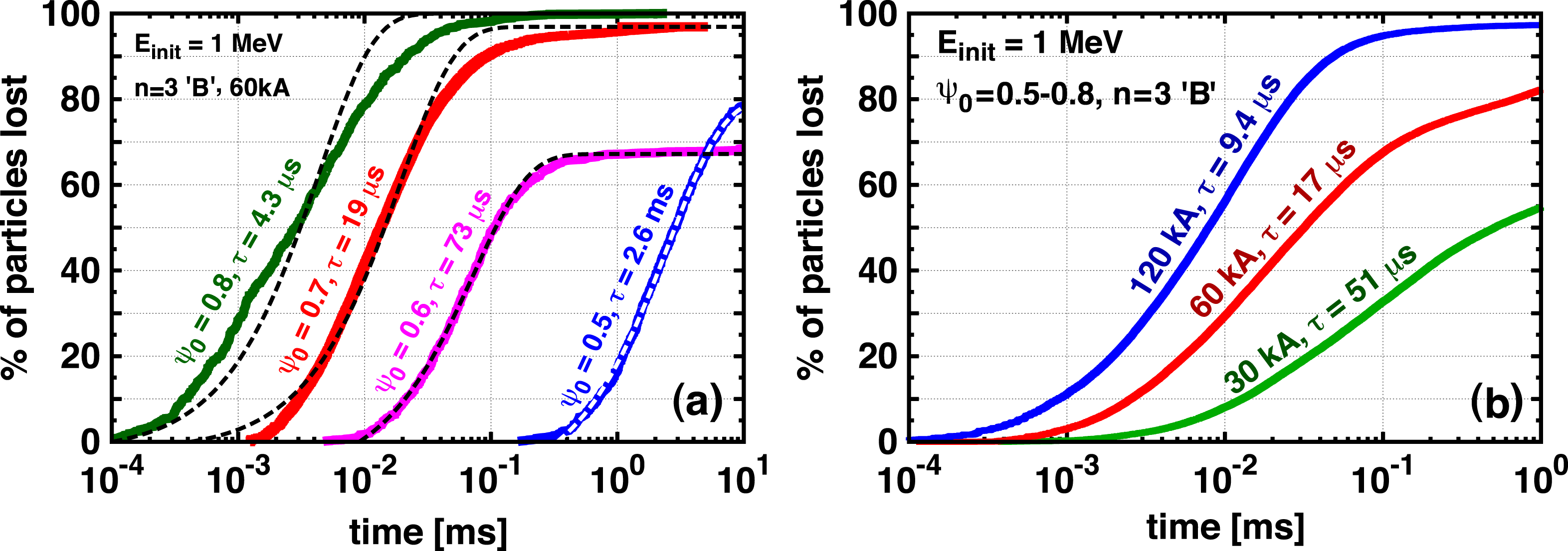
Despite this complexity, the ensemble behaviour is smooth. Figure 2(a) shows the fraction of lost particles as a function of time for particles launched at individual flux surfaces. All these curves show an exponential decay of the confined particles up to the saturation value, determined by the fraction of particles trapped in remnant O-points of an island chain intersecting the starting surface. Dashed lines show exponential fits, and the characteristic loss times are indicated above the curves.

Figure 2.

(a) Fraction of lost particles for different starting radii as a function of time. Dashed lines show $N_{lost}(t)=N_{0}(1-\exp \{-t/{\it\tau}\})$ fits. (b) Fraction of lost particles within ${\it\psi}\in [0.5,0.8]$ for different perturbation currents as a function of time.

The magnetic-perturbation-enhanced net radial transport leads to particle losses on the sub-millisecond time scale. Our energy scans confirmed that on this short time scale the behaviour is similar regardless of the energy of the particles if $E>1~\text{MeV}$ , as the particles mainly follow the open magnetic field lines with the speed $v_{\Vert }\simeq c$ . The long-term ( ${>}10~\text{ms}$ ) behaviour is determined by the remnant island structures. Particles starting in specific spatial positions can be trapped in the remnant O-points and confined even at energies of 100 MeV.

If the magnetic perturbation strength is increased (by increasing the current in the coils), the island structure will change nonlinearly. Therefore, the relationship between the time evolution of the losses and the magnetic perturbation magnitude is not trivial. Figure 2(b) illustrates the fraction of lost particles as a function of time for three different values of the perturbation current. To highlight the effect of the magnetic perturbation magnitude, in these simulations the electric field has been set to zero (the electrons are not accelerated as they were in the other simulations).

The smooth ensemble behaviour is also reflected in the evolution of the electron density as a function of radial position ( ${\it\psi}$ ) and time, as is shown in figure 3(a). The continuous radial loss picture is only distorted by the enhanced confinement of the remnant island chains at ${\it\psi}=0.5$ , 0.6 and 0.7. For comparison, figure 3(b) shows the evolution of density due to the Rechester–Rosenbluth diffusion for the same initial conditions. The evolution of the density, $n({\it\psi},t)$ , is largely different: the diffusive model predicts better confinement at the edge but worse confinement in the core, by orders of magnitudes. The generation of runaway electrons is exponentially sensitive to the existing number of runaways through the avalanche process. If instead of a test particle scenario the runaway electron generation is included in the calculation, the differences between the two cases are increased even further, as will be shown later in this paper.

Figure 3.

(a) Evolution of the fast electron density $n({\it\psi},t)$ as calculated by the ANTS code. (b) Evolution of the density due to Rechester–Rosenbluth diffusion. Both figures are calculated for 60 kA coil current.

Following the observations illustrated in figures 2(a,b) and 3(a), we approximated the particle losses with an $N_{lost}(t)\propto 1-\exp \{-t/{\it\tau}({\it\psi})\}$ trend, where ${\it\tau}({\it\psi})$ is the characteristic loss time associated with a certain initial ${\it\psi}$ position for the particles. We have performed fits of ${\it\tau}({\it\psi})$ to the evolution of fast electron density obtained by the 3D test particle simulations for various cases, such as the ones illustrated in figures 2(a,b) and 3(a). The fitted values of ${\it\tau}({\it\psi})$ are shown in figure 4(b) for three different perturbation magnitudes. We note that the dependence of ${\it\tau}({\it\psi})$ on the radial coordinate is relatively smooth and is well approximated by an exponential dependence ${\it\tau}({\it\psi})\propto \exp \{-{\it\psi}/{\it\psi}_{0}\}$ (dashed lines), where ${\it\psi}_{0}\propto {\it\delta}B/B$ . Local maxima in ${\it\tau}({\it\psi})$ correspond to remnant islands and KAM zones in the perturbed magnetic topology.

Figure 4.

(a) Evolution of electron density using the fitted ${\it\tau}({\it\psi})$ values for the 60 kA configuration, including particles confined in the remnant islands ( $n_{c}$ ). (b) Fitted values of ${\it\tau}$ as a function of normalized flux for three different perturbation amplitudes.

By replacing the diffusive transport in a numerical calculation with the exponential loss model, we can calculate the evolution of fast particle density using the fitted ${\it\tau}({\it\psi})$ values. A pure exponential loss description cannot reproduce the confined fraction. However, if we split the particle density into a confined and a non-confined fraction, $n({\it\psi},t)=n_{c}({\it\psi})+n_{nc}({\it\psi},t)$ , where the confined part is constant at a given radial position (extracted from the ANTS simulations) and the non-confined part follows the exponential loss $n_{nc}(t,{\it\psi})\propto 1-\exp \{-t/{\it\tau}({\it\psi})\}$ , we can reproduce the results of the 3D simulation. Figure 4(a) shows a calculation based on the exponential losses for the 60 kA case, including the $n_{c}({\it\psi})$ particles confined in the remnant islands. It clearly resembles the particle evolution calculated by ANTS (figure 3 a – the figures are placed next to each other for easier comparison).

3. Self-consistent calculations

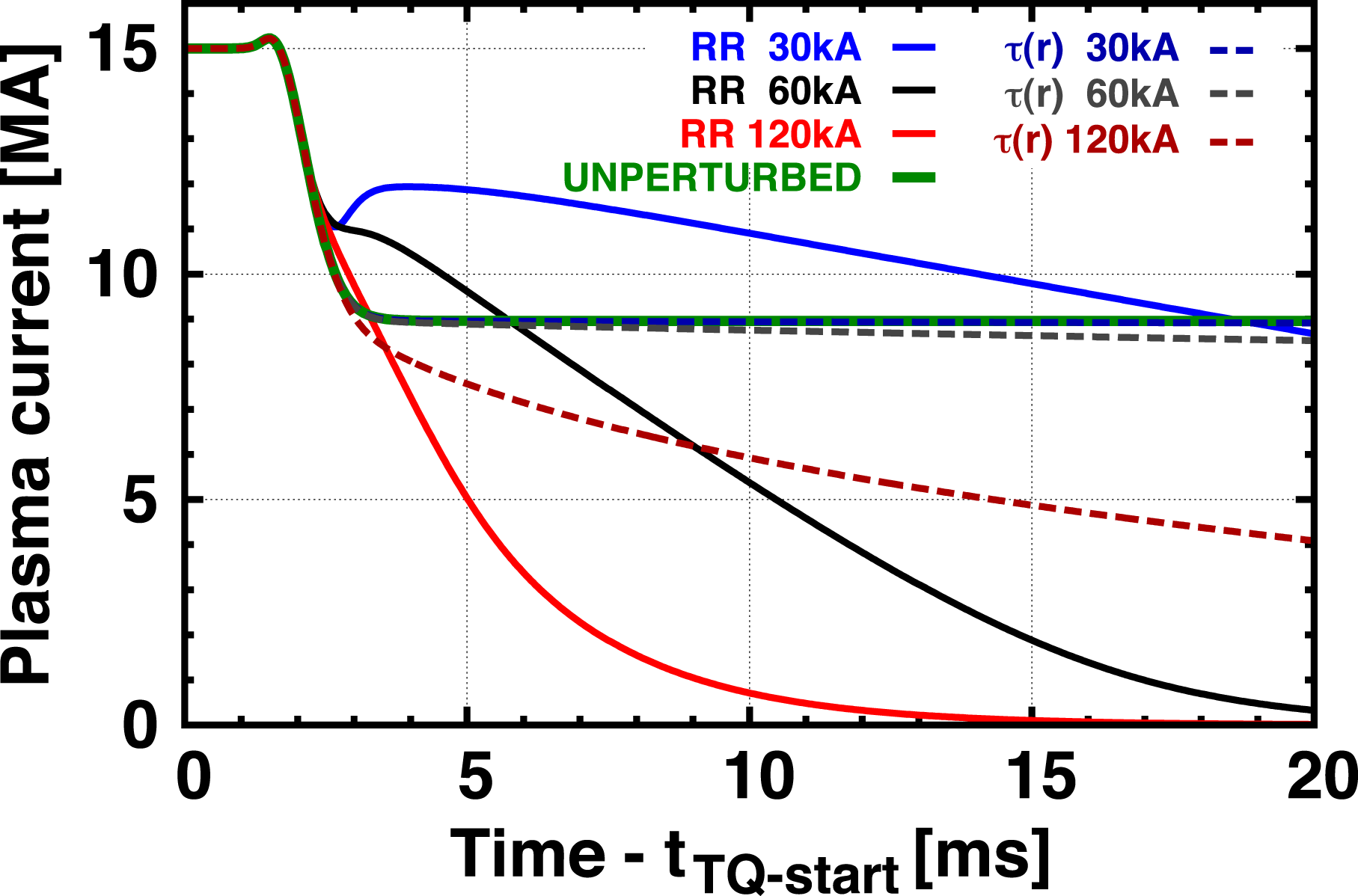
To illustrate the differences between the implications of the diffusive and exponential-loss models, we have implemented both loss models in a self-consistent simulation of the runaway current and electric field evolution (Papp et al. Reference Papp, Fülöp, Fehér, de Vries, Riccardo, Reux, Lehnen, Kiptily, Plyusnin and Alper2013). Figure 5 shows a disruption simulation for the same ITER scenario as was used for the 3D simulations. The thermal quench time is set to 0.2 ms and the effective charge $Z_{eff}=2$ to mimic the parameter evolution of massive gas injection simulations (Papp et al. Reference Papp, Fülöp, Fehér, de Vries, Riccardo, Reux, Lehnen, Kiptily, Plyusnin and Alper2013; Hollmann et al. Reference Hollmann, Aleynikov, Fülöp, Humphreys, Izzo, Lehnen, Lukash, Papp, Pautasso, Saint-Laurent and Snipes2015). As a general conclusion for all cases, following the thermal collapse, at ${\sim}3~\text{ms}$ virtually all of the Ohmic current is replaced by runaways, and the runaway current consists of ${\sim}10\,\%$ seed and ${\sim}90\,\%$ avalanche current. Without losses a runaway beam of ${\sim}9~\text{MA}$ would form. Using the Rechester–Rosenbluth diffusion model and the ${\it\delta}B/B$ profile caused by the perturbation coils we get suppression of the runaways after 20 ms at $I_{RMP}=60~\text{kA}$ and after 10 ms at $I_{RMP}=120~\text{kA}$ . The current $I_{RMP}=30~\text{kA}$ not only does not lead to suppression, but through the redistribution of the primary seed current leads to temporary stronger avalanching, increasing the overall runaway current. However, as we argue in this paper, with the support of the 3D test particle calculations, the losses in these systems are not well described by diffusion. Moreover, the simulations show that although the perturbation penetrates to the core, the transport is essentially untouched inside the radius $r/a=0.7$ for $I_{RMP}=60~\text{kA}$ . Therefore, even if the transport is greatly increased towards the edge region in the exponential loss description, this does not contribute much to runaway suppression. The reason is that most of the runaways are formed in the plasma core, where there is good runaway confinement according to the test particle simulations. As the dashed lines in figure 5 clearly illustrate, virtually no runaway suppression is achieved even at $I_{RMP}=60$  kA with the exponential loss model. At $I_{RMP}=120~\text{kA}$ we see a slow drop of the runaway current, however, $I_{RMP}>75~\text{kA}$ will not be accessible in ITER due to hardware limitations.

Figure 5.

Effect of diffusive (solid lines) versus exponential (dashed lines) losses on plasma (runaway electron) current evolution for ITER in a self-consistent calculation for different perturbation strengths.