





1. Introduction
Understanding the influence of turbulence on the transport of heat and other scalar properties in stably stratified flows is a major challenge in geophysical and environmental fluid dynamics (Simpson & Hunter Reference Simpson and Hunter1974; Bormans & Webster Reference Bormans and Webster1997). Comprehending stably stratified turbulence near boundaries is also essential for various industrial applications, including heat transfer processes in energy systems (Pitla et al. Reference Pitla, Robinson, Groll and Ramadhyani1998; Zonta et al. Reference Zonta, Marchioli and Soldati2008). Stable stratification, resulting from density differences associated with temperature and/or salinity gradients, significantly affects many environmental phenomena, such as the stratified atmospheric boundary layer (Mahrt Reference Mahrt1999, Reference Mahrt2014), turbulent mixing and the movement of organic species in rivers and the ocean (Simpson & Hunter Reference Simpson and Hunter1974; Bormans & Webster Reference Bormans and Webster1997; Wunsch & Ferrari Reference Wunsch and Ferrari2004). In water bodies, solar radiation is absorbed through the water column following the Beer–Lambert law, creating a stable stratification that suppresses turbulent mixing near the surface. During the day, this reduced mixing limits the transport of dissolved oxygen and nutrients, potentially leading to hypoxia and fish deaths near the bottom (Erskine et al. Reference Erskine, Turner, Terrazzolo and Warner1999; Turner & Erskine Reference Turner and Erskine2005). Additionally, stratification promotes cyanobacteria growth, which harms water quality by producing cyanotoxins that can threaten aquatic ecosystems and human health (Webster et al. Reference Webster, Sherman, Bormans and Jones2000; Turner & Erskine Reference Turner and Erskine2005).
The behaviour of turbulent wall-bounded flows under stable stratification is governed by the opposition of buoyancy and shear forces. On one hand, the vertical movement of fluid extracts turbulent kinetic energy from the mean shear flow. On the other hand, this vertical transport must work against stratification effects, consuming potential energy in the process (García-Villalba & del Álamo Reference García-Villalba and del Álamo2011). The interplay between these forces can vary across different wall-normal distances due to the statistical inhomogeneity of wall turbulence, creating a complex spatial structure. This variation can lead to the emergence of distinct flow regions: some areas are characterised by elongated velocity streaks where shear effects dominate, while others display prominent features controlled by buoyancy forces (García-Villalba & del Álamo Reference García-Villalba and del Álamo2011). In thermally stratified turbulent flows, turbulence drives temperature fluctuations through turbulent convection, while temperature fluctuations influence turbulence via mean temperature gradients and density changes (Feng et al. Reference Feng, Liu, Liu and Zheng2024). The detailed structures of velocity and temperature fields in fully developed flows help unravel the complexities of turbulent momentum and heat transport (Hishida & Nagano Reference Hishida and Nagano1979).
Consequently, numerous efforts have been made to simulate stably stratified turbulent flows, aiming to explore stratification regimes and the suppression of turbulence. Stratification can be introduced in various ways, one of which is by imposing a fixed temperature difference between the upper and lower walls. This approach has been widely used in previous studies on stratified channel flows. For instance, Armenio & Sarkar (Reference Armenio and Sarkar2002) employed large-eddy simulation to examine stratified full-channel flows (flows bounded by walls on both the upper and lower surfaces) at a Prandtl number (
 $ \textit{Pr}$
) of
 $0.71$
and friction Reynolds number
 $ \textit{Re}_{\tau }$
of
 $180$
, under a constant density difference across the channel. Their results showed that as stratification increases (higher friction Richardson number in their study), the buoyancy-influenced zone progressively extends into the turbulent inner layer. Under the strongest stratification considered, the coherent low-speed streaks characteristic of near-wall turbulence are diminished. Similarly, direct numerical simulations (DNS) of open-channel (flows bounded by a solid bottom and a free surface at the top) (Nagaosa & Saito Reference Nagaosa and Saito1997) and full-channel flows (Garg et al. Reference Garg, Ferziger, Monismith and Koseff2000) demonstrated turbulence suppression with increasing stratification. A reduction in the root-mean-square (r.m.s.) velocity fluctuations was observed in the near-wall region due to decreased turbulence kinetic energy production as stratification intensifies (Garg et al. Reference Garg, Ferziger, Monismith and Koseff2000). The study concluded that stratification disrupts the characteristic pattern of alternating high- and low-speed streaks near the wall in buoyancy-dominated flows. Additionally, strong stratification diminishes the coupling between the inner and outer regions by limiting vertical momentum and energy transport, effectively isolating the two layers under sufficiently intense stratification (Garg et al. Reference Garg, Ferziger, Monismith and Koseff2000).
García-Villalba & del Álamo (Reference García-Villalba and del Álamo2011) investigated full-channel flows at higher friction Reynolds number (
 $ \textit{Re}_{\tau }= 550$
in addition to
 $180$
) and stratification level compared with previous works with
 $ \textit{Pr}=0.71$
, finding that weak stratification minimally affects near-wall turbulence, while strong stratification results in laminarisation throughout the channel. Under strong stratification, large laminar regions form throughout the channel, extending all the way to the wall. As stratification increases, turbulent shear stresses decrease significantly in the core of the channel, approaching nearly zero in strongly stratified cases. This reduction allows the flow to accelerate, resulting in higher mean velocities.
Regarding the temperature field, buoyancy exerts a stronger influence on the temperature structure in the outer region than in the inner region (García-Villalba & del Álamo Reference García-Villalba and del Álamo2011). This influence suppresses the formation of large-scale temperature patterns, as observed in the two-dimensional premultiplied spectra of density. Similarly, Zonta et al. (Reference Zonta, Sichani and Soldati2022) observed that at
 $ \textit{Re}_{\tau } = 1000$
, buoyancy effects dominate in regions with reduced mean shear, even at low to moderate stratification levels. Further studies (Iida et al. Reference Iida, Kasagi and Nagano2002; Feng et al. Reference Feng, Liu, Liu and Zheng2024) highlighted reduced turbulent heat flux and enhanced mean temperature gradients under stratification with
 $ \textit{Pr}=0.71$
. Additionally, the scale of temperature fluctuations at the channel centre decreases, signifying a substantial reduction in heat mixing due to turbulence (Iida et al. Reference Iida, Kasagi and Nagano2002). Intermittent regions have also been observed in stratified flows, manifesting as laminar spots that emerge, grow and dissipate within the flow (Iida et al. Reference Iida, Kasagi and Nagano2002). Feng et al. (Reference Feng, Liu, Liu and Zheng2024) also indicated that under stable stratification, the scale size of velocities and temperature is less than that under neutral conditions. Moreover, thermal buoyancy significantly influences the temperature structure under stable stratification. They observed that near the wall, temperature fluctuations exhibit morphological characteristics similar to those of streamwise velocity structures in both stable and neutral stratifications. As the wall-normal position increases, the streamwise length of temperature structures diminishes, while their volume increases linearly. The study also revealed that stable stratification suppresses the scale sizes of streamwise velocity and temperature farther away from the wall compared with neutral conditions. However, the temperature scales remain larger than those of streamwise velocity at greater distances from the wall at constant
 $ \textit{Pr}=0.71$
.
It is also important which thermal boundary condition used at the free surface of the half-channel flows. Handler et al. (Reference Handler, Saylor, Leighton and Rovelstad1999) investigated open-channel flow by applying Neumann and Dirichlet conditions at the free surface and compared their effects on passive scalar behaviour. Their findings revealed that the variations in surface flux were significantly greater under the Dirichlet condition compared with the variations in surface concentration observed with the Neumann condition. Additionally, the scalar field exhibited distinct structural differences at the free surface depending on which boundary condition was imposed. Under Neumann conditions (constant flux), the surface temperature field exhibited large patches of warm fluid. Kawamura et al. (Reference Kawamura, Ohsaka, Abe and Yamamoto1998) performed DNS of channel flow at
 $ \textit{Re}_{\tau }=180$
with a constant time-averaged heat-flux condition. Similarly, Pirozzoli et al. (Reference Pirozzoli, Bernardini and Orlandi2016) investigated passive scalar transport in turbulent closed-channel flows and highlighted the contrasts between uniform volumetric forcing (heat source, as used here) and fixed-scalar differences. While near-wall behaviour (e.g.
 $y/h \lesssim 0.2$
or
 $y^{+} \lesssim 100$
) is broadly similar between the two, substantial differences arise in the outer region (
 $y/h \gtrsim 0.2$
) and core (
 $y/h \gtrsim 0.5$
–
 $0.6$
). In the fixed-scalar differences case, strong core eddies emerge, resembling those in turbulent Couette flow, which enhance outer-layer activity. Such findings emphasise that volumetric heating produces fundamentally different turbulence characteristics, particularly in the outer layer, compared with simpler boundary conditions.
Studies involving fixed temperature walls (reviewed above) can be comparable to atmospheric surface boundary layers experiencing intense surface cooling (Taylor et al. Reference Taylor, Sarkar and Armenio2005). In such cases, a negative heat flux (cooling) at the ground suppresses turbulence generation in the bottom surface layer. Another method of introducing stratification is by applying heat flux at the top or bottom boundary or using a volumetric heat source. Studies that applied a heat flux at the top (Taylor et al. Reference Taylor, Sarkar and Armenio2005) or a volumetric heat source that is not uniform throughout the channel and varies in the wall-normal direction (that is greater in strength near the free surface) (Williamson et al. Reference Williamson, Armfield, Kirkpatrick and Norris2015; Jahani et al. Reference Jahani, MacDonald and Norris2024) observed that the near-wall region is mostly unaffected by stratification in contrast to most of the studies that used a fixed temperature difference (Nagaosa & Saito Reference Nagaosa and Saito1997; Garg et al. Reference Garg, Ferziger, Monismith and Koseff2000; Armenio & Sarkar Reference Armenio and Sarkar2002). This is due to the minimal heat flux (from a non-uniform volumetric heat source) near the wall and the adiabatic bottom boundary, resulting in a small temperature difference in that region. The distinction between a fixed-temperature wall and a heat-flux wall lies in the near-wall temperature fluctuations: at a fixed-temperature wall, they are zero at the wall, whereas at a heat-flux wall, they have a finite, non-zero value. Also, the temperature variance differs between the two configurations, showing a near-wall peak for fixed temperature difference, whereas our results agree with Taylor et al. (Reference Taylor, Sarkar and Armenio2005), who reported no such peak. It is notable that the boundary conditions of heat flux at the top free surface and an adiabatic bottom wall are more relevant to environmetal water flows, such as an ocean thermocline formed by surface heating in shallow water on nearly uniform depth (Taylor et al. Reference Taylor, Sarkar and Armenio2005). However, the studies reviewed above focused on turbulent stratified flows using a fixed temperature difference as the boundary condition.
Williamson et al. (Reference Williamson, Armfield, Kirkpatrick and Norris2015) used DNS to simulate a turbulent stratified flow in an open channel, with heating that decreases exponentially with depth, modelled according to the Beer–Lambert law (defined in § 2). Their findings for
 $ \textit{Pr}=0.71$
revealed that as stratification intensifies, the mean streamwise velocity and temperature profiles near the free surface increase, while velocity and temperature fluctuations, turbulent shear stress and turbulent heat flux in that region decrease significantly. They found that in steady state, the turbulence within the central region of the flow achieves a state of local energetic equilibrium. In this balanced state, the shear production of turbulent kinetic energy is offset by the combined effects of buoyancy destruction and viscous dissipation. Recent DNS studies of stratified open-channel flow by Issaev et al. (Reference Issaev, Williamson, Armfield and Norris2022, Reference Issaev, Williamson and Armfield2023) adopted the same flow configuration as that of Williamson et al. (Reference Williamson, Armfield, Kirkpatrick and Norris2015), using
 $ \textit{Pr}=1$
. Issaev et al. (Reference Issaev, Williamson and Armfield2023) examined the spatiotemporal intermittency in such flows. They stated that the flow exhibits spontaneous intermittency, marked by the formation of a horizontal interface that separates the laminar upper layer from the turbulent lower layer. This interface is shaped by intense mixing driven by ‘overturning’ shear instabilities. Recently, Jahani et al. (Reference Jahani, MacDonald and Norris2024) conducted a DNS simulation to model stratified open-channel flow subjected to a radiative volumetric heat source modelled by the Beer–Lambert law, for a range of
 $0.07 \leqslant \textit{Pr} \leqslant 7$
, showing that
 $ \textit{Pr}$
affects the mean and turbulence characteristics of the flow. It was shown that increasing
 $ \textit{Pr}$
in the flow with the same stability parameter leads to flow acceleration and a rise in temperature in the upper part of the channel. Additionally, higher
 $ \textit{Pr}$
suppresses turbulent shear stress and heat flux near the free surface. In stratified flow with
 $ \textit{Pr}=7$
, an analysis of Reynolds stresses and turbulent heat flux shows significant turbulence suppression near the free surface compared with lower Prandtl numbers (Jahani et al. Reference Jahani, MacDonald and Norris2024).
Previous studies have shown that stable stratification significantly affects the behaviour of turbulent channel flows by analysing mean flow and one-point statistics. In contrast, few studies have investigated two-point statistical measures, such as velocity and temperature spectra (García-Villalba & del Álamo Reference García-Villalba and del Álamo2011) or two point correlations (Feng et al. Reference Feng, Liu, Liu and Zheng2024), both of which used a fixed temperature gradient between walls in full-channel flows.
Furthermore, due to computational resource limitations, most DNS-based studies of turbulent stratified flows have been conducted with fluids having a Prandtl number less than or equal to 1, which does not realistically represent water (
 $ \textit{Pr}=7$
). Nonetheless, these studies have provided valuable insights and significantly advanced our understanding of the problem. This is despite evidence indicating that the Prandtl number plays a significant role in stratified turbulence (Legaspi & Waite Reference Legaspi and Waite2020; Okino & Hanazaki Reference Okino and Hanazaki2020; Jahani et al. Reference Jahani, MacDonald and Norris2024). Therefore, more research on stratified open-channel flows with boundary conditions more relevant to environmental water flows is needed to better understand the effects of stratification on both large and small scales within the flow.
Unlike our previous work (Jahani et al. Reference Jahani, MacDonald and Norris2024), which investigated only the mean characteristics of the flow for
 $0 \leqslant \gamma _{0} \leqslant 0.5$
and
 $0.07 \leqslant \textit{Pr} \leqslant 7$
, the present research extends the DNS simulations to stratification bulk parameters up to
 $\gamma _{0}=2$
, which creates stronger level of stratification, for
 $ \textit{Pr}$
of 0.71. The bulk stability parameter,
 $\gamma _{0}$
, is defined as the ratio between the wall-normal length (channel height) and a bulk Obukhov length scale for the flow (Williamson et al. Reference Williamson, Armfield, Kirkpatrick and Norris2015), serving as a measure of stratification strength and quantifying the relative influence of buoyancy forces to shear forces in the flow. Additionally, two-point statistics are analysed to reveal the detailed influences of stratification on energy spectra and spatial organisation of turbulence throughout the channel for
 $ \textit{Pr}=0.71$
and 7. This represents a central contribution of the study, as such a comparison has not, to the best of our knowledge, been previously reported in stratified open-channel flows. In contrast to the widely investigated configuration with differentially heated boundaries, the present study employs DNS of a stratified open-channel flow driven by a radiative volumetric heat source described by the Beer–Lambert law. This formulation is especially relevant to naturally heated water bodies subject to radiative forcing, but has so far been explored only to a limited extent in the existing literature. The presence of a free surface in open-channel flows plays a crucial role in shaping turbulence dynamics, promoting the development of stronger large-scale motions and influencing the distribution of turbulent kinetic energy (Yao et al. Reference Yao, Chen and Hussain2022). In this respect, the physical problem considered here is directly relevant to environmental applications.
The paper is organised as follows. In § 2 we outline the physics of stratification, along with the governing equations and boundary conditions. The numerical methodology is described in § 3. In § 4 we present the discussion of the results. In § 4.1 we focus on the mean streamwise velocity and temperature profiles, as well as one-point statistics. In § 4.2, the premultiplied spanwise spectra of velocity and temperature fluctuations are analysed to examine how energy is distributed across different scales. The temperature variance budget equation is discussed in § 4.3. To identify the turbulence scales, two-point correlations and integral length scales in the spanwise direction are analysed in § 4.4. In § 4.5 we provide detailed insights into the probability distribution of velocity and temperature fluctuations using flatness and skewness profiles. Finally, the conclusions of this study are summarised in § 5.
2. Problem formulation
This study adopts the thermally stratified open-channel flow framework described by Williamson et al. (Reference Williamson, Armfield, Kirkpatrick and Norris2015) and Jahani et al. (Reference Jahani, MacDonald and Norris2024). The computational domain includes a no-slip adiabatic bottom wall and a free-slip, adiabatic top boundary, with periodic conditions applied in the streamwise (
 $x$
) and spanwise (
 $z$
) directions (figure 1). The variable
 $y$
represents the wall-normal direction. The flow is driven by a constant pressure gradient in the streamwise direction. Solar radiation is represented as a volumetric heat source based on the Beer–Lambert law, decreasing exponentially with depth,
 \begin{align} q_{r}(y) = I_{s} K_{d} e^{K_{d}(y-h)}, \end{align}
where
 $h$
is the channel height,
 $I_{s}$
represents the radiant heat flux entering through the top surface and
 $K_{d}$
is the absorption coefficient that accounts for turbidity effects. The turbidity parameter,
 $K_{d} h$
, controls the vertical distribution of radiative heating and therefore influences the level of stratification near the bottom surface. It characterises the attenuation of radiation intensity as it penetrates the fluid. In all simulations,
 $K_{d} h$
is fixed at 8, consistent with previous studies (Williamson et al. Reference Williamson, Armfield, Kirkpatrick and Norris2015; Kirkpatrick et al. Reference Kirkpatrick, Williamson, Armfield and Zecevic2019; Issaev et al. Reference Issaev, Williamson, Armfield and Norris2022, Reference Issaev, Williamson and Armfield2023, Reference Issaev, Armfield and Williamson2025; Nguyen-Dang et al. Reference Nguyen-Dang, Williamson, Armfield, Kirkpatrick and Norris2023). At this value, the volumetric heating decreases substantially with depth, and the heating near the bottom surface is negligible compared with the surface value.
Computational domain and boundary conditions. The domain is periodic in the
 $x$
and
 $z$
directions.

The flow becomes statistically stationary after an initial transient period, allowing decomposition of the dimensional temperature field (
 $T$
) into a spatial average (
 $\bar {T}$
) and a fluctuating component (
 $T^{\prime }$
) (Lei & Patterson Reference Lei and Patterson2002, Reference Lei and Patterson2003; Williamson et al. Reference Williamson, Armfield, Kirkpatrick and Norris2015; Jahani et al. Reference Jahani, MacDonald and Norris2024):
 \begin{align} T(\hat {x}, \hat {y}, \hat {z}, \hat {t}) = \bar {T}(\hat {t}) + T^{\prime }(\hat {x}, \hat {y}, \hat {z}, \hat {t}). \end{align}
Here,
 $\hat {x}$
,
 $\hat {y}$
and
 $\hat {z}$
denote the spatial coordinates in dimensional form, and
 $\hat {t}$
represents the dimensional time. Then,
 $x$
,
 $y$
,
 $z$
and
 $t$
are corresponding non-dimensional values normalised by
 $h$
and
 $h/u_{\tau }$
, respectively. Radiative heating causes the spatially averaged temperature to rise over time. The rate of this increase is expressed as
 ${\rm d} \bar {T}/{\rm d}\hat {t}= \bar {q_{r}}/\rho _{0} c_{p}$
, where
 $\rho _{0}$
and
 $c_{p}$
denote the fluid density and specific heat capacity, respectively. The average volumetric heat source and representative heat source, respectively, are defined as
 \begin{align} \bar {q_{r}} = \frac {1}{h} \int _{0}^{h} q_{r}(\hat {y}) \,{\rm d}\hat {y} = \frac {I_{s}}{h}(1-e^{-K_{d}h}), \\[-28pt] \nonumber \end{align}
 \begin{align} q_{N} = \frac {1}{h^{2}} \int _{0}^{h} (\bar {q_{r}}- q_{r}(\hat {y})) (h - \hat {y}) \,{\rm d}\hat {y} , \\[0pt] \nonumber \end{align}
where for high
 $K_{d}h$
we can obtain
 \begin{align} q_{N} \approx \frac {I_{s}}{h} \left(\frac {1}{2}- \frac {1}{K_{d}h} \right)\! . \end{align}
The temperature deviation
 $T^{\prime }(\hat {x}, \hat {y}, \hat {z}, \hat {t})$
is statistically steady and horizontally homogeneous. The non-dimensional form of the temperature deviation field,
 $\theta$
, and the volumetric heat source,
 $q_{e}$
, are defined as
 \begin{align} \theta (x, y, z, t) = \frac {T(\hat {x}, \hat {y}, \hat {z}, \hat {t}) - \bar {T}(\hat {t})}{T_{N}}, \quad T_{N} = \frac {q_{N} h}{\rho _{0} c_{p} u_{\tau }}, \\[-28pt] \nonumber \end{align}
 \begin{align} q_{e}(y) = \frac {q_{r}(\hat {y}) - \bar {q_{r}}}{q_{N}}. \\[0pt] \nonumber\end{align}
Stratification effects are characterised by the bulk stability parameter
 $\gamma _{0}$
, derived from the Obukhov length scale
 $\mathbb{L}$
, (Williamson et al. Reference Williamson, Armfield, Kirkpatrick and Norris2015),
 \begin{align} \gamma _{0} = \frac {h}{\mathbb{L}}, \quad \mathbb{L} =\frac {u^{3}_{\tau }}{g \beta q_{N} h / \rho _{0} c_{p}} = \frac {u^{3}_{\tau }}{g \beta I_{s} / \rho _{0} c_{p}}\left (\frac {1}{2}-\frac {1}{K_{d} h}\right )^{-1}\!, \end{align}
where
 $\beta$
is the thermal expansion coefficient and
 $g$
is gravitational acceleration.
The governing equations include the incompressible Navier–Stokes and thermal energy equations under the Boussinesq approximation, with buoyancy incorporated via the stability parameter
 $\gamma _{0}$
. The equations are presented in their non-dimensional form as follows:
 \begin{align} \frac {\partial u_i}{\partial x_i} = 0, \\[-28pt] \nonumber \end{align}
 \begin{align} \frac {\partial u_i}{\partial t} + u_{\kern-1pt j} \frac {\partial u_i}{\partial x_{\kern-1pt j}} = -\frac {\partial p}{\partial x_i} + \frac {1}{Re_{\tau }} \frac {\partial ^2 u_i}{\partial x_{\kern-1pt j}^2} + G \delta _{i1} + \gamma _{0} \theta \delta _{i2}, \\[-28pt] \nonumber \end{align}
 \begin{align} \frac {\partial \theta }{\partial t} + u_{\kern-1pt j} \frac {\partial \theta }{\partial x_{\kern-1pt j}} = \frac {1}{Re_{\tau } \textit{Pr}} \frac {\partial ^2 \theta }{\partial x_{\kern-1pt j}^2} + q_e, \\[-12pt] \nonumber \end{align}
where
 $ \textit{Re}_{\tau } = u_{\tau } h / \nu$
is the friction Reynolds number, and
 $ \textit{Pr}$
is the Prandtl number. Here,
 $u_{\tau }$
is the friction velocity,
 $\nu$
is the kinematic viscosity and
 $p$
is the pressure. The source term
 $\gamma _{0} \theta$
in the momentum equation represents the buoyancy force due to thermal stratification. The spatial coordinate
 $x_{j}$
is scaled by the channel height
 $h$
. The velocity field
 $u_{j}$
is normalised by the friction velocity,
 $u_{\tau }=\sqrt {\tau _{w}/\rho }=\sqrt {\nu {\rm d}u/{\rm d}y }_{|{y=0}}$
. The viscous length is defined as
 $l_{\tau }=\nu / u_{\tau }$
. The viscosity and thermal diffusivity are normalised by
 $u_{\tau } h$
, time by
 $h/u_{\tau }$
, and pressure by
 $\rho _{0} u^{2}_{\tau }$
. Here,
 $\delta _{ij}$
denotes the Kronecker delta. The flow is driven by a constant pressure gradient
 $G$
in the
 $x$
direction. In a neutrally stratified statistically steady state of an open-channel flow,
 $G$
explicitly determines the friction velocity
 $u_{\tau }$
. Under the present non-dimensionalisation,
 $u_{\tau }= \sqrt {G}$
.
Boundary conditions enforce a no-slip and adiabatic bottom wall, while the top surface is free-slip and adiabatic, with the domain being periodic in the other directions.
In this study, instantaneous variables are denoted as
 $u$
,
 $v$
,
 $w$
for the velocity components, and
 $\theta$
for the temperature field. Through Reynolds decomposition, these instantaneous fields are split into two parts: the mean flow (indicated by
 $\bar {\boldsymbol{\cdot }}$
) and fluctuating fields (shown by
 $\boldsymbol{\cdot }^\prime$
). This gives us expressions like
 $u = {\bar {u}} + u^{\prime }$
and
 $\theta = {\bar {\theta }} + \theta ^{\prime }$
.
After an initial transient period of
 $40{-}50$
non-dimensional time units (
 $\hat {t}u_{\tau }/h$
), the system reaches a statistically steady state. Once this is achieved, data are averaged over at least
 $40$
non-dimensional time units. The statistically steady conditions of the flow is verified by ensuring that the r.m.s. fluctuations of velocity and temperature converge to their mean values. During the steady state, flow statistics are computed by averaging across horizontal planes (i.e. periodic directions) and over time, denoted by the angle bracket,
 $\langle \boldsymbol{\cdot }\rangle$
.
3. Numerical methodology
The simulations used the in-house non-staggered finite volume solver SnS (Norris Reference Norris2000; Armfield et al. Reference Armfield, Morgan, Norris and Street2003), which integrates the governing equations using a fractional step method. The solver uses second-order central differencing for spatial terms. The time integration of the equations was performed using a fractional-step approach (Armfield & Street Reference Armfield and Street2000). In this method, the advection and the diffusion terms were discretised with a second-order Adams–Bashforth and a Crank–Nicolson scheme, respectively (Armfield & Street Reference Armfield and Street2002). A variable time step was used to ensure the Courant number remained below
 $0.24$
, with a stricter limit of
 $0.2$
applied to cases with the higher Prandtl number (
 $ \textit{Pr}=7$
). The Courant number is computed based on the grid used for the momentum equations. For the multiresolution cases, the time step is correspondingly refined using the same factor as the mesh refinement to maintain scalar stability on the finer grid. Therefore, the Courant number is identical for both the momentum and temperature equations.
In DNS, the mesh size must be fine enough to capture the smallest turbulent scales in the momentum and temperature fields. The smallest velocity scales are of the order of the Kolmogorov scale,
 $\eta _{K}=(\nu ^{3}/\epsilon )^{1/4}$
, where
 $\epsilon =\nu \langle (\partial u^{\prime }_{i}/\partial x_{j})^{2} \rangle$
is the turbulent pseudodissipation rate (Pope Reference Pope2000). However, the smallest temperature scales are of the order of the Batchelor scale (Batchelor Reference Batchelor1959), given by
 $\eta _{B}=\eta _{K}/\sqrt {Pr}$
. Consequently, fluids with
 $ \textit{Pr} \gt 1$
require a finer mesh than the velocity field to resolve temperature variations accurately. To mitigate the increased computational demands, a multiresolution method was used (Dahmen et al. Reference Dahmen, Gottschlich-Müller and Müller2001; Li & Li Reference Li and Li2004; Ostilla-Monico et al. Reference Ostilla-Monico, Yang, Van Der Poel, Lohse and Verzicco2015; Chong et al. Reference Chong, Ding and Xia2018). This technique uses a higher resolution for the temperature field while maintaining a coarser mesh for the momentum and pressure fields.
In the current study, for high
 $ \textit{Pr}$
cases, a multiresolution approach is employed to capture the finer thermal field scales without unnecessarily resolving the momentum and pressure fields. At each time step, the velocity and temperature fields are interpolated (a quadratic interpolation method described by Chong et al. (Reference Chong, Ding and Xia2018)) between the coarse and fine grids to ensure mass conservation. This method significantly reduces the simulation time for higher
 $ \textit{Pr}$
cases while maintaining accuracy (Ostilla-Monico et al. Reference Ostilla-Monico, Yang, Van Der Poel, Lohse and Verzicco2015). Jahani et al. (Reference Jahani, MacDonald and Norris2024) reported that the multiresolution approach reduced the computational cost of simulations by a factor of approximately 11 compared with the single-resolution method, resulting in a substantial saving in wall-clock time. Further details can be found in the earlier studies by Jahani et al. (Reference Jahani, MacDonald and Norris2022, Reference Jahani, MacDonald and Norris2024).
The vertical grid spacing is refined near the walls (because of sharp velocity gradients) and in regions of sharp thermal gradients (near the top surface) to capture small-scale dynamics, especially under strong stratification. The simulation parameters and the number of grid cells for each case are presented in table 1. For
 $ \textit{Pr} = 0.71$
, the mesh resolutions of the momentum field and the temperature field are the same and follows the configuration as that of Williamson et al. (Reference Williamson, Armfield, Kirkpatrick and Norris2015), while for
 $ \textit{Pr} = 7$
, the mesh resolution for the temperature field is halved, i.e.
 $n = 2$
. For cases with
 $\gamma _{0} \leqslant 0.5$
, the mesh spacing in the streamwise and spanwise directions is uniform, with
 $\Delta x^{+}=10$
(
 $N_{x}=256$
) and
 $\Delta z^{+}=5$
(
 $N_{z}=256$
), respectively. For cases with
 $\gamma _{0}=1$
and 2, the streamwise resolution is refined to
 $\Delta x^{+}=4.6$
(
 $N_{x}=540$
). Validation was carried out in our previous study (Jahani et al. Reference Jahani, MacDonald and Norris2024), where stratified flow cases with
 $ \textit{Pr}=0.71$
and
 $\gamma _{0}=0.5$
and
 $1$
were compared with the data of Williamson et al. (Reference Williamson, Armfield, Kirkpatrick and Norris2015) at
 $ \textit{Re}_{\tau }=395$
. The results showed good agreement with the benchmark values. For stratified flow with
 $ \textit{Pr} = 7$
, a thin thermal boundary layer forms near the top surface, requiring mesh refinement in the vertical direction. For
 $ \textit{Pr} = 7$
with
 $\gamma _{0} \gt 0$
, vertical grid spacing ranges from
 $\Delta y^{+} = 0.4$
to
 $2.6$
, with grid spacing reduced to
 $\Delta y^{+} = 0.8$
at the top surface (
 $N_{y} = 200$
), while the mesh for the temperature field is halved. The Kolmogorov length scale,
 $\eta _{K}^{+} = \eta _{K}/l_{\tau }$
, expressed in terms of viscous wall units, ranges from
 $1.5$
near the bottom wall to
 $5.7$
near the top surface for
 $ \textit{Pr} \leqslant 0.71$
, and
 $1.5$
to
 $8.4$
for
 $ \textit{Pr} = 7$
. Correspondingly, the Batchelor scale,
 $\eta _{B}^{+}$
, spans from
 $0.57$
to
 $3.2$
at
 $ \textit{Pr} = 7$
. As discussed by Moin & Mahesh (Reference Moin and Mahesh1998), although the Kolmogorov length scale (
 $\eta _{K}$
) is commonly cited as the smallest scale that must be resolved, it is generally sufficient to resolve scales of the order of
 $\eta _{K}$
(i.e.
 $\Delta y \lesssim O(\eta _{K})$
) to capture most of the dissipation. Our mesh resolution meets this criterion throughout the domain, with the ratio
 $\Delta y / \eta _{K}$
ranging from approximately 0.2 near the bottom wall to 1.7 in the midchannel, and decreasing to around 0.5 near the top surface. Since the Batchelor scale is defined in terms of
 $\eta _{K}$
as
 $\eta _{B}=\eta _{K}/\sqrt {Pr}$
, a comparable resolution requirement naturally extends to
 $\eta _{B}$
. With the refinement factor used here, the ratio
 $\Delta y / (n \eta _{B})$
ranges from 0.1 to 2.2 for the neutral case, and from 0.1 to 1.2 for the stratified cases (see Appendix B). As the Kolmogorov and Batchelor length scales vary with wall-normal distance, we provide the worst-case grid sizes (Maryada et al. Reference Maryada, Armfield, Dhopade and Norris2023).
Simulation parameters. Here
 $n$
is the multiresolution refinement factor.

Table 1. Long description
The table presents simulation parameters and the number of grid cells for each case. It has 8 rows and 8 columns. The columns are labeled Pr, Reτ, Lx, Lz, γ0, Nx, Ny, Nz, and n. The rows provide specific values for these parameters. Row 1: Pr, 0.71; Reτ, 395; Lx, Lz, 2π, π; γ0, 0.0; Nx, 256; Ny, 110; Nz, 256; n, 1. Row 2: Pr, 0.71; Reτ, 395; Lx, Lz, 2π, π; γ0, 0.1; Nx, 256; Ny, 110; Nz, 256; n, 1. Row 3: Pr, 0.71; Reτ, 395; Lx, Lz, 2π, π; γ0, 0.5; Nx, 256; Ny, 110; Nz, 256; n, 1. Row 4: Pr, 0.71; Reτ, 395; Lx, Lz, 2π, π; γ0, 1.0; Nx, 540; Ny, 130; Nz, 256; n, 1. Row 5: Pr, 0.71; Reτ, 395; Lx, Lz, 2π, π; γ0, 2.0; Nx, 540; Ny, 130; Nz, 256; n, 1. Row 6: Pr, 7.0; Reτ, 395; Lx, Lz, 2π, π; γ0, 0.0; Nx, 256; Ny, 110; Nz, 256; n, 2. Row 7: Pr, 7.0; Reτ, 395; Lx, Lz, 2π, π; γ0, 0.1; Nx, 256; Ny, 200; Nz, 256; n, 2. Row 8: Pr, 7.0; Reτ, 395; Lx, Lz, 2π, π; γ0, 0.5; Nx, 256; Ny, 200; Nz, 256; n, 2.
Initial conditions for stratified flow cases are derived from lower
 $\gamma _{0}$
cases at statistical equilibrium, following established practices in the literature by Armenio & Sarkar (Reference Armenio and Sarkar2002), García-Villalba & del Álamo (Reference García-Villalba and del Álamo2011) and Zonta et al. (Reference Zonta, Sichani and Soldati2022). A laminar parabolic velocity profile in a half-channel flow was used as the initial condition for
 $\gamma _{0}=0$
. Simulations are run until statistical steady-state conditions are achieved. The reader is referred to Jahani et al. (Reference Jahani, MacDonald and Norris2024) for further information.
4. Results and discussion
The main objective of this research is to investigate the energy content and structure of stratified flows under different stability regimes at various spatial scales. To accomplish this, we examine the mean flow characteristics, one-point statistics, energy spectra and two-point correlation for fully stratified open-channel flows at Prandtl numbers of
 $0.71$
and
 $7$
, along with varying bulk stability parameter
 $\gamma _{0}$
values from
 $0$
to
 $2$
.
4.1. Mean profiles and one-point statistics
First, we focus on the mean flow and one-point statistics (figure 2), briefly summarising the relevant findings of Jahani et al. (Reference Jahani, MacDonald and Norris2024) for comparison and helping in interpreting subsequent sections. We extend the analysis to higher
 $\gamma _{0}$
, where notable differences emerge. We then proceed to examine the spectra and two-point statistics.
Mean streamwise velocity (a,e), the streamwise velocity fluctuations (b,f), mean temperature (c,g) and normalised temperature fluctuations (d,h) against wall-normal position. Panels (a)–(d) show variations of
 $\gamma _{0}$
at
 $ \textit{Pr}=0.71$
, and panels (e)–(h)show
 $\gamma _{0}=0.5$
at
 $ \textit{Pr}=0.71$
and
 $ \textit{Pr}=7$
.

Figure 2. Long description
The image contains eight line graphs arranged in two rows and four columns. Each graph shows data trends against wall-normal position. Panel A: A line graph showing mean streamwise velocity against wall-normal position. The x-axis is labeled with the mean streamwise velocity, and the y-axis is labeled with wall-normal position. Different line styles represent various initial conditions. Panel B: A line graph showing streamwise velocity fluctuations against wall-normal position. The x-axis is labeled with streamwise velocity fluctuations, and the y-axis is labeled with wall-normal position. Different line styles represent various initial conditions. Panel C: A line graph showing mean temperature against wall-normal position. The x-axis is labeled with mean temperature, and the y-axis is labeled with wall-normal position. Different line styles represent various initial conditions. Panel D: A line graph showing normalized temperature fluctuations against wall-normal position. The x-axis is labeled with normalized temperature fluctuations, and the y-axis is labeled with wall-normal position. Different line styles represent various initial conditions. Panel E: A line graph showing mean streamwise velocity against wall-normal position. The x-axis is labeled with the mean streamwise velocity, and the y-axis is labeled with wall-normal position. Different line styles represent various Prandtl numbers. Panel F: A line graph showing streamwise velocity fluctuations against wall-normal position. The x-axis is labeled with streamwise velocity fluctuations, and the y-axis is labeled with wall-normal position. Different line styles represent various Prandtl numbers. Panel G: A line graph showing mean temperature against wall-normal position. The x-axis is labeled with mean temperature, and the y-axis is labeled with wall-normal position. Different line styles represent various Prandtl numbers. Panel H: A line graph showing normalized temperature fluctuations against wall-normal position. The x-axis is labeled with normalized temperature fluctuations, and the y-axis is labeled with wall-normal position. Different line styles represent various Prandtl numbers.
In all simulations, the flow is driven by a constant pressure gradient. The velocity
 $(u, v , w)$
is normalised by the friction velocity, and so is equal to
 $(u^{+}, v^{+}, w^{+})$
, where
 $+$
denotes that the variables are expressed in terms of viscous wall units. In thermally stratified turbulent channel flow, buoyancy forces significantly influence vertical turbulent transport and the conversion of energy between turbulent kinetic energy and potential energy (Williamson et al. Reference Williamson, Armfield, Kirkpatrick and Norris2015; Kirkpatrick et al. Reference Kirkpatrick, Williamson, Armfield and Zecevic2019). In these flows, the temperature field acts as an active scalar, dynamically interacting with the velocity field. Figure 2(a) illustrates mean streamwise velocity profiles for various stability parameters,
 $\gamma _{0}$
, at
 $ \textit{Pr}=0.71$
. As
 $\gamma _{0}$
increases from
 $0$
to
 $2$
, the flow velocity increases in the upper part of the channel. From figure 2(e), comparing the mean streamwise velocity at
 $\gamma _{0}=0.5$
for
 $ \textit{Pr}=0.71$
and
 $ \textit{Pr}=7$
, reveals that this increase results in higher velocities near the free surface for
 $ \textit{Pr}=7$
. This occurs due to a significant reduction in turbulent shear stress coupled with an increase in viscous shear stress (Jahani et al. Reference Jahani, MacDonald and Norris2024). The increased mean streamwise velocity is attributed to a decrease in the skin friction coefficient, which increases the bulk mean velocity while the wall friction velocity remains constant (Williamson et al. Reference Williamson, Armfield, Kirkpatrick and Norris2015).
Stratification is known to inhibit turbulent mixing near the free surface and alters the turbulence structure throughout the channel, in our case this is even more pronounced away from the bottom wall. However, the shear is dominant near the wall and the thermal stratification is only significant towards the top surface due to the definition of the heat source (figure 1), which is negligible near the bottom wall. As a result, stratification does not noticeably affect the mean velocity profile near the bottom wall (figure 2 a,e). This finding is consistent with previous studies of stratified open-channel flows with the same configuration (Williamson et al. Reference Williamson, Armfield, Kirkpatrick and Norris2015), as well as with studies using different configurations in which a fixed mean vertical temperature gradient or a constant heat flux was imposed at the boundaries (Nieuwstadt Reference Nieuwstadt2005; Taylor et al. Reference Taylor, Sarkar and Armenio2005; Wang & Lu Reference Wang and Lu2005; Flores & Riley Reference Flores and Riley2011; Xiao & Senocak Reference Xiao and Senocak2022).
Figure 2(b) indicates the r.m.s. of velocity fluctuations for different
 $\gamma _{0}$
values. A similar plot, comparing
 $\langle u^{\prime }u^{\prime } \rangle ^{1/2}$
at
 $\gamma _{0}=0.5$
for
 $ \textit{Pr}=0.71$
and
 $ \textit{Pr}=7$
, is presented in figure 2(f). These figures show that stratification, characterised by varying
 $\gamma _{0}$
and
 $ \textit{Pr}$
, has negligible impact on the mean velocity fluctuations near the wall.
In the middle part of the channel (
 $0.2 \lesssim y \lesssim 0.8$
), as the stability parameter increases to 1 and 2, the streamwise velocity fluctuations reach larger values. This increase is attributed to the steeper mean streamwise velocity gradient, which contributes to the increased turbulent production term. Additionally, as
 $\gamma _{0}$
increases, the influence of buoyancy forces on the mean flow extends farther into lower wall-normal locations. However, when
 $ \textit{Pr}$
changes from 0.71 to 7 at the same
 $\gamma _{0}=0.5$
, the primary effects are observed near the free surface. As shown in figure 2(f),
 $\langle u^{\prime }u^{\prime } \rangle ^{1/2}$
remains largely unchanged up to
 $y=0.5$
. In contrast, increasing
 $ \textit{Pr}$
significantly impacts the mean flow near the free surface, effectively suppressing turbulence intensities more strongly.
It should be noted that the suppression of turbulent kinetic energy and turbulence near the free surface, stratified open channel flows is attributed to stratification effects. Multiple DNS studies of free-slip open-channel flows have consistently demonstrated the persistence of turbulence near the free surface, even in the absence of direct production. These works show that turbulence is sustained through redistribution and transport mechanisms, rather than local production alone (Handler et al. Reference Handler, Swean, Leighton and Swearingen1993; Komori et al. Reference Komori, Nagaosa, Murakami, Chiba, Ishii and Kuwahara1993; Calmet & Magnaudet Reference Calmet and Magnaudet2003; Duan et al. Reference Duan, Chen, Li and Zhong2020; Peruzzi et al. Reference Peruzzi, Poggi, Ridolfi and Manes2020; Yao et al. Reference Yao, Chen and Hussain2022). Our results for the neutral condition (
 $\gamma _{0}=0$
) are therefore consistent with the established understanding that turbulence exists near the free surface of free-slip open channels, even though its dynamics differ fundamentally from those at no-slip boundaries.
For the strongly stratified cases, the reduction in turbulence near the free surface is not merely a uniform weakening of turbulent fluctuation magnitudes, but may also be indicative of turbulence intermittency. In wall-bounded stratified flows, under sufficiently strong stabilising buoyancy, the flow can partially relaminarise, leading to the coexistence of turbulent and non-turbulent phases (Armenio & Sarkar Reference Armenio and Sarkar2002; García-Villalba & del Álamo Reference García-Villalba and del Álamo2011; Deusebio et al. Reference Deusebio, Caulfield and Taylor2015; Issaev et al. Reference Issaev, Williamson, Armfield and Norris2022, Reference Issaev, Williamson and Armfield2023). It is examined in more detail in §§ 4.4 and 4.5.
Figures 2(c,g) and 2(d,h) illustrate the normalised mean temperature and r.m.s. of temperature fluctuations against non-dimensional wall-normal position, respectively. Normalisation is performed using the incident surface flux
 $I_{s}/hq_{N}$
(Williamson et al. Reference Williamson, Armfield, Kirkpatrick and Norris2015; Jahani et al. Reference Jahani, MacDonald and Norris2024).
Under stable stratification, thermal buoyancy suppresses velocity fluctuations near the top surface, as evident in the
 $u^{+}_{\textit{rms}}$
profile shown in figure 2(b,f) as well as in
 $v^{+}_{\textit{rms}}$
and
 $w^{+}_{\textit{rms}}$
, as reported by Jahani et al. (Reference Jahani, MacDonald and Norris2024). This suppression of velocity fluctuations, along with reduced vertical turbulent transport due to buoyancy effects, leads to higher mean temperatures and steeper temperature gradients near the free surface. Additionally, the increase in the thermal production term of the temperature variance budget equation with increasing
 $\gamma _{0}$
and
 $ \textit{Pr}$
, which will be discussed in § 4.3, is accompanied by a steeper mean temperature gradient. An increase in the temperature fluctuations in the upper part of the channel is observed in regions of higher temperature gradient, which then drop significantly close to the top surface at
 $\gamma _{0}=1$
and
 $2$
due to the suppression of turbulence by buoyancy effects (figure 2
d). A similar trend has been reported in the DNS of stratified open-channel flows by Williamson et al. (Reference Williamson, Armfield, Kirkpatrick and Norris2015). In contrast, most earlier investigations have described different thermal structures. For example, Komori et al. (Reference Komori, Ueda, Ogino and Mizushina1983) conducted experiments with steam condensation at the free surface, while Garg et al. (Reference Garg, Ferziger, Monismith and Koseff2000) and Wang & Lu (Reference Wang and Lu2005) studied cases with an isothermal free surface and either adiabatic or isothermal bottom boundaries. Deusebio et al. (Reference Deusebio, Schlatter, Brethouwer and Lindborg2011) considered a configuration with a fixed temperature difference imposed across the channel. More recently, Xiao & Senocak (Reference Xiao and Senocak2022) carried out DNS to explore the stabilising influence of two stratification mechanisms, a constant negative surface buoyancy flux and a prescribed ambient stratification, acting independently or simultaneously on an initially neutral flow.
At higher
 $ \textit{Pr}$
, the mean temperature profile reaches larger values (figure 2
g). This is due to the reduced thermal diffusivity, which results in a narrower thermal boundary layer and limits heat conduction towards the near wall region. Consequently, temperature fluctuations rise sharply before being significantly suppressed near the surface (figure 2
h).
4.2. Energy spectra
Section 4.1 presented profiles that assess the impact of stratification on turbulence levels within channel flows. However, it is not clear how stratification affects the spatial organisation of the turbulence structure.
Premultiplied spanwise spectral densities of streamwise velocity fluctuations with wall-normal distance. The shaded contours are the simulations for
 $ \textit{Pr}=0.71$
under (a) neutral conditions (
 $\gamma _{0}=0$
), (b)
 $\gamma _{0}=0.1$
, (c)
 $\gamma _{0}=0.5$
, (d)
 $\gamma _{0}=1$
and (e)
 $\gamma _{0}=2$
. There are 10 equally spaced contours ranging from 0 to 4. The black solid/dashed lines correspond to the positive/negative values (0.15, −0.15) of
 $(E_{uu,\gamma _{0}}-E_{uu,0})$
. The blue line represents the Ozmidov length scale (
 $l_{O}^{+}$
).

In wall-bounded turbulent flows like the stratified open-channel flow in our study, spanwise spectra sufficiently characterise energy-containing eddy structures. As shown by Hwang (Reference Hwang2015), premultiplied spanwise spectra of streamwise velocity reveal a distinct linear ridge at
 $y \approx 0.1 \lambda _z$
in the logarithmic region, evidencing self-similar attached eddies that scale with wall distance and connect near-wall (
 $ \lambda _z^+ \approx 100$
) to outer motions (
 $ \lambda _z \approx 1.5h$
). Streamwise spectra do not exhibit a clear ridge; instead, they reflect elongated projections of spanwise scales (e.g.
 $ \lambda _x \approx 10 \lambda _z$
for streaks,
 $ 2$
–
 $3 \lambda _z$
for shorter vortices). Consequently, analysing the spanwise spectra alone is sufficient to capture the self-similarity and scaling, without redundancy from streamwise projections.
Following Hwang (Reference Hwang2015), the spanwise spectra of velocity and temperature are used to analyse how energy is distributed across various scales. For completeness, the streamwise energy spectra of the streamwise velocity fluctuations for the representative case
 $ \textit{Pr}=0.71$
are also presented in Appendix C. The spanwise spectra
 $E_{aa}$
for a fluctuating field
 $a$
is defined as
 \begin{align} \langle a^{\prime } a^{\prime } \rangle = \int _{1}^{\infty } k_{z}E_{aa}(k_{z}) \, {\rm d}(\log k_{z})= \int _{0}^{\infty } E_{aa}(k_{z}) \, {\rm d}(k_{z}) ,\end{align}
where
 $k_{z}$
is the spanwise wavenumber and
 $\langle a^{\prime } a^{\prime } \rangle$
denotes the variance of
 $a^{\prime }$
. Figure 3 illustrates the spanwise spectra of the streamwise velocity fluctuations for different
 $\gamma _{0}$
values for
 $ \textit{Pr}=0.71$
, plotted as a function of wavelength and wall-normal position. Figure 3 displays the energy spectra across all wall-normal positions on a logarithmic scale, with 10 evenly spaced contour levels ranging from 0 to 4. The energy spectra, consistent with prior studies (Hutchins & Marusic Reference Hutchins and Marusic2007; Lee & Moser Reference Lee and Moser2015), show a peak at
 $y^{+} \approx 15$
with a spanwise wavelength of
 $\lambda ^{+}_{z} \approx 100$
, matching the typical spacing of near-wall streaks (Kline et al. Reference Kline, Reynolds, Schraub and Runstadler1967). The energy content of the buffer layer streaks remains largely unaffected by stratification (figure 3
a
 $-$
e).
The difference between two spectra,
 $(E_{uu,\gamma _{0}}-E_{uu,0})$
(using the same approach as Li et al. (Reference Li, De Silva, Chung, Pullin, Marusic and Hutchins2021)), indicates the decrease or increase in the energy content under stratified conditions compared with neutral conditions at different wavelengths and wall-normal positions. Here,
 $E_{uu,0}$
and
 $E_{uu,\gamma _{0}}$
denote the spanwise energy spectra of
 $u$
for neutral conditions and stratified conditions (
 $\gamma _{0}=0.1$
, 0.5, 1, 2), respectively. The black lines in figure 3 show this difference. Figure 3(a
 $-$
e) illustrate that as
 $\gamma _{0}$
increases, the energy associated with large wavelengths diminishes:
 $\lambda ^{+}_{z} \gtrsim 500$
(
 $\lambda _{z} / h \gtrsim 1.26$
) for
 $\gamma _{0}=0.1$
,
 $\lambda ^{+}_{z} \gtrsim 400$
(
 $\lambda _{z} / h \gtrsim 1.01$
) for
 $\gamma _{0}=0.5$
,
 $\lambda ^{+}_{z} \gtrsim 400$
for
 $\gamma _{0}=1$
, and
 $\lambda ^{+}_{z} \gtrsim 300$
(
 $\lambda _{z} / h \gtrsim 0.76$
) for
 $\gamma _{0}=2$
. This reduction happens over
 $0.025 \lt y \lt 0.55$
for
 $\gamma _{0}=0.1$
and extends deeper into the buffer layer, as
 $\gamma _{0}$
increases. For
 $\gamma _{0}=2$
, it is evident that energy content also decreases at
 $200 \lesssim \lambda ^{+}_{z} \lesssim 300$
over
 $10 \lesssim y^{+} \lesssim 22$
. However, the wavelengths with the most energy content in the buffer layer remain largely unchanged, and the peak of
 $\langle u^{\prime }u^{\prime } \rangle ^{1/2}$
, which occurs in the buffer layer, does not alter. Noting that while
 $\lambda _{z} / h$
may indeed be a more appropriate scaling at large wavelengths (see figures 3 and 4), our analysis is limited to a single friction Reynolds number and therefore does not permit a broader generalisation. A larger domain or higher Reynolds number would allow improved understanding on the wavelengths and their associated scaling; accordingly, the reported scales should be regarded as approximate.
Considering the mean flow velocity, Taylor et al. (Reference Taylor, Sarkar and Armenio2005) demonstrated that in stratified open-channel flows with a heat flux at the top and an adiabatic bottom wall, stratification has a negligible impact on the near wall region and buffer layer compared with cases with a fixed temperature difference across the channel (Nagaosa & Saito Reference Nagaosa and Saito1997; Armenio & Sarkar Reference Armenio and Sarkar2002). Figure 2(b,f) similarly indicate that the streamwise velocity fluctuations,
 $\langle u^{\prime }u^{\prime } \rangle ^{1/2}$
, remain unchanged near the bottom wall, with the maximum values being consistent across all cases. As will be shown later, the energy content at
 $y^{+}=15$
remains unaffected by increases in
 $\gamma _{0}$
and Prandtl number up to
 $\lambda ^{+}_{z} \approx 300$
(
 $\lambda _{z} / h \approx 0.76$
). While the mean streamwise velocity profiles do not exhibit significant differences near the wall under stratified flow conditions, the energy spectra (figures 3 and 4) reveal that stratification influences the large scales deeper into the buffer layer. However, since large scales contribute only marginally to the energy content near the wall, their influence on the mean flow profiles remains minimal.
In contrast to the near wall region, the influence of large wavelengths is more pronounced in the upper part of the channel as
 $\gamma _{0}$
increases. This is because over
 $y \gtrsim 0.75$
, large scales are more dominant in terms of energy content. Near the free surface, the energy content associated with large spanwise structures (
 $ \lambda ^{+}_{z} \gtrsim 400$
–
 $500$
,
 $\lambda _{z} / h \gtrsim 1.26$
−
 $1.01$
) diminishes substantially, particularly at
 $\gamma _{0}=2$
(figure 3
e), and this reduction leads to a marked weakening of the overall energy content in that region.
As stratification intensifies, energy levels at smaller wavelengths in the range
 $ 80 \lesssim \lambda ^{+}_{z} \lesssim 320$
(
 $0.2 \lesssim \lambda _{z} / h \lesssim 0.81$
) increase in the top part of the channel, particularly below
 $y=0.75$
. For
 $\gamma _{0}=0.5$
, energy spectra rise in the range
 $ 200 \lesssim \lambda ^{+}_{z} \lesssim 310$
(
 $0.5 \lesssim \lambda _{z} / h \lesssim 0.78$
) over
 $0.3 \lt y \lt 0.75$
(figure 3
c). These regions expand with increasing stability (figure 3
d,e), and at
 $\gamma _{0}=2$
, a broader range of smaller wavelengths,
 $80 \lesssim \lambda ^{+}_{z} \lesssim 310$
(
 $0.2 \lesssim \lambda _{z} / h \lesssim 0.78$
), becomes more energetic over a wider range of wall-normal positions
 $0.1 \lt y \lt 0.72$
(figure 3
e).
Premultiplied spanwise spectral densities of streamwise velocity with wall-normal distance. The shaded contours are the simulation for
 $ \textit{Pr}=7$
under (a)
 $\gamma _{0}=0$
, (b)
 $\gamma _{0}=0.1$
and (c)
 $\gamma _{0}=0.5$
. There are 10 equally spaced contours ranging from 0 to 4. The black solid/dashed lines correspond to the positive/negative values (0.15, −0.15) of
 $(E_{uu,\gamma _{0}}-E_{uu,0})$
. The blue line represents the Ozmidov length scale (
 $l_{O}^{+}$
).

Figure 4. Long description
Three contour plots depict premultiplied spanwise spectral densities of streamwise velocity with wall-normal distance. Each plot represents different conditions. Panel A shows the simulation for a specific condition with 10 equally spaced contours ranging from 0 to 4. The black solid and dashed lines correspond to the positive and negative values of a specific parameter. The blue line represents the Ozmidov length scale. Panel B and Panel C follow the same structure as Panel A, each showing the simulation under different conditions with the same contour ranges and line representations. The contour plots illustrate how the spectral densities vary with wall-normal distance under different thermal boundary conditions, highlighting differences in the scalar field and turbulence characteristics.
One of the key novel outcomes of the present study lies in the comparison of energy spectra between
 $ \textit{Pr} = 0.71$
and
 $ \textit{Pr} = 7$
, which, to our knowledge, has not been reported in previous studies of stratified open-channel flows. Turning now to the higher
 $ \textit{Pr}=7$
scenario, figure 4 presents the premultiplied spanwise spectra of the streamwise velocity fluctuations for neutral conditions and for
 $ \textit{Pr} = 7$
at
 $\gamma _{0}=0.1$
and 0.5. The findings indicate that stratification only affects larger wavelengths close to the wall at
 $ \textit{Pr}=7$
, similar to what is seen at
 $ \textit{Pr}=0.71$
. However, in the upper part of the channel, stratification alters the energy distribution across different wavelengths and wall-normal locations. At a given
 $\gamma _{0}$
, the reduction of energy at large wavelengths (
 $\lambda ^{+}_{z} \gtrsim 500$
,
 $\lambda _{z} / h \gtrsim 1.26$
) penetrates more deeply into the buffer layer and extends farther towards the free surface at
 $ \textit{Pr} = 7$
compared with
 $ \textit{Pr} = 0.71$
. Moreover, in the upper region, stratification at
 $ \textit{Pr} = 7$
affects a broader range of wavelengths, with notable changes across both large and intermediate scales. While the loss of energy at large wavelengths (
 $\lambda ^{+}_{z} \gtrsim 500$
) is broadly comparable between the two Prandtl numbers, with slightly stronger reductions at
 $ \textit{Pr} = 7$
, the redistribution at smaller wavelengths differs more substantially. Specifically, at
 $\gamma _{0}=0.5$
, a wider band of smaller wavelengths (
 $120 \lesssim \lambda ^{+}_{z} \lesssim 340$
,
 $0.3 \lesssim \lambda _{z} / h \lesssim 0.86$
) over
 $0.3 \lt y \lt 0.75$
gains energy at
 $ \textit{Pr} = 7$
, whereas the corresponding changes at
 $ \textit{Pr} = 0.71$
are confined to a narrower spectral range. A similar trend has been reported in studies with different flow configurations. Feng et al. (Reference Feng, Liu, Liu and Zheng2024), in their investigation of turbulent structures under stable stratification in a fixed-temperature-difference closed-channel flow, observed a reduction in the size of eddies in the core region, indicating that most of the turbulent energy shifts towards smaller scales. Likewise, García-Villalba & del Álamo (Reference García-Villalba and del Álamo2011) showed from streamwise velocity spectra that, at
 $y^{+}=100$
and in the channel core, stratification damps the large-scale motions, and a greater concentration of energy is observed at smaller scales. These consistent observations support our finding that stable stratification preferentially suppresses energy at large wavelengths while distributing energy towards smaller scales.
Our observations indicate that stratification primarily affects large scales, leading to a reduction in energy at large wavelengths (
 $\lambda ^{+}_{z} \gtrsim 500$
,
 $\lambda _{z} / h \gtrsim 1.26$
). This behaviour is also reported by García-Villalba & del Álamo (Reference García-Villalba and del Álamo2011) in stratified flows. However, they had different temperature boundary conditions, suggesting that this behaviour is not solely related to thermal boundary conditions. Similar behaviour has been documented in the atmospheric surface layer, where Kaimal et al. (Reference Kaimal, Wyngaard, Izumi and Coté1972) and Kaimal & Finnigan (Reference Kaimal and Finnigan1994) showed that stable stratification suppresses energy in the low-frequency (large-scale) components of the turbulence spectrum. Large-eddy simulations of the stable boundary layer by Huang & Bou-Zeid (Reference Huang and Bou-Zeid2013) further confirmed that stronger stratification reduces integral length scales and weakens turbulent motions. More recently, Heisel et al. (Reference Heisel, Sullivan, Katul and Chamecki2023) reported that with increasing stability, turbulence becomes weaker, more intermittent, and increasingly dominated by smaller scales. Our results show that the scales in the range
 $300 \lesssim \lambda ^{+}_{z} \lesssim 500$
are increasingly affected under stronger stratification, which arises from higher
 $\gamma _{0}$
or the enhanced stratification effects observed at higher
 $ \textit{Pr}$
, leading to a significant energy reduction in these scales. This suggests that the large spanwise wavelengths are more sensitive to buoyancy effects.
Flow structures with scales larger than the Ozmidov length,
 $l_{O}=(\epsilon / N^{3})^{(1/2)}$
, are significantly influenced by buoyancy forces (Chung & Matheou Reference Chung and Matheou2012; Williamson et al. Reference Williamson, Armfield, Kirkpatrick and Norris2015), where
 $N$
is the buoyancy frequency. In this study, the Ozmidov length scale (
 $l_{O}^{+}=l_{O}/ l_{\tau }$
) is plotted (blue line in figures 3 and 4) alongside the energy spectra to provide a reference for the largest turbulent eddies unaffected by buoyancy, thereby allowing a direct assessment of how stratification constrains turbulent motions. The trend shown in figure 3 indicates that, in strongly stratified flows, almost all scales are influenced near the top of the channel. As stratification increases, the Ozmidov length decreases throughout the channel. It takes values of
 $l_{O}^{+}=800$
,
 $430$
and
 $280$
viscous units for
 $\gamma _{0}=0.5$
,
 $1$
and
 $2$
, respectively, in the region
 $10 \lesssim y^{+} \lesssim 50$
. The results suggest that the energy content is closely associated with the Ozmidov scale, which, under strong stratification, provides an approximate threshold above which buoyancy effects become significant. For higher values of
 $\gamma _{0}$
,
 $l_{O}^{+}$
decreases further, implying that stratification may begin to affect scales of the order of 100 viscous units, smaller than the buffer-layer peak in the spanwise spectra reported by García-Villalba & del Álamo (Reference García-Villalba and del Álamo2011), potentially influencing shear production close to the wall. A similar overall trend is observed at higher Prandtl numbers (figure 4). However, the decrease in
 $l_{O}^{+}$
is more pronounced at higher
 $ \textit{Pr}$
for a given
 $\gamma _{0}$
, indicating that a greater portion of turbulence is suppressed.
Premultiplied spanwise spectra of streamwise velocity at different
 $\gamma _{0}$
and wall-normal locations: (a)
 $y^{+}=15$
, (b)
 $y=0.5$
, (c)
 $y=0.7$
, (d)
 $y=0.9$
.

Figure 5 provides a detailed comparison of the premultiplied spectra of streamwise velocity fluctuations for open channel flows across a range of stability conditions (
 $\gamma _{0}=0$
to
 $2$
) at different wall-normal locations for
 $ \textit{Pr}=0.71$
and
 $ \textit{Pr}=7$
. The blue- and red-shaded lines in figure 5 represent the cases with
 $ \textit{Pr}=0.71$
and
 $ \textit{Pr}=7$
, respectively. The results highlight that in the region away from the bottom wall (starting from
 $y \gt 0.3$
; not shown here), smaller-wavelength structures become increasingly dominant in terms of energy content as stability (
 $\gamma _{0}$
) strengthens. This behaviour is shown in figure 5(b
 $-$
d) at
 $y=0.5$
,
 $y=0.7$
and
 $y=0.9$
, where energy shifts from larger to smaller wavelengths, resulting in the energy peaks in the region away from the bottom wall to occur at shorter wavelengths. For instance, at
 $y=0.5$
, the energy peak shifts from
 $\lambda ^{+}_{z} \approx 600$
(
 $\lambda _{z} / h \approx 1.52$
) for
 $\gamma _{0}=0$
to
 $\lambda ^{+}_{z} \approx 200$
(
 $\lambda _{z} / h \approx 0.5$
) for
 $\gamma _{0}=2$
. This trend is even more pronounced at
 $y=0.7$
, where the energy peak decreases from
 $\lambda ^{+}_{z} \approx 600$
(
 $\lambda _{z} / h \approx 1.52$
) for
 $\gamma _{0}=0$
to
 $\lambda ^{+}_{z} \approx 130$
(
 $\lambda _{z} / h \approx 0.33$
) for
 $\gamma _{0}=2$
. This aligns with our observations from figure 3(c
 $-$
e), which show an increase in energy content at those smaller scales at the relevant locations as the stability parameter increases. This behaviour can be attributed to the suppression of large-scale motions by buoyancy forces (García-Villalba & del Álamo Reference García-Villalba and del Álamo2011), which reduces the vertical transport of momentum and energy. Consequently, smaller structures carry a greater proportion of energy in the flow under strongly stratified conditions compared with the case with lower
 $\gamma _{0}$
.
To highlight the influence of Prandtl number, we now compare the higher Prandtl number case (
 $ \textit{Pr} = 7$
) with the reference case (
 $ \textit{Pr} = 0.71$
). At
 $\gamma _{0}=0.1$
, the differences in energy content between
 $ \textit{Pr}=0.71$
and
 $ \textit{Pr}=7$
are negligible. However, at
 $\gamma _{0}=0.5$
, noticeable differences emerge, particularly at
 $y=0.7$
and
 $y=0.9$
. From figure 5(b), it can be observed that the energy content in the middle of the channel (
 $y=0.5$
) is nearly the same for
 $ \textit{Pr}=0.71$
and
 $ \textit{Pr}=7$
at
 $\gamma _{0}=0.5$
. However, at the higher wall-normal position of
 $y=0.7$
, the energy associated with wavelengths in the range
 $\lambda ^{+}_{z} \lesssim 220$
is significantly enhanced in the high-
 $ \textit{Pr}$
case, increases more for
 $ \textit{Pr}=7$
than for
 $ \textit{Pr}=0.71$
.
Moreover, near the free surface (
 $y=0.9$
), the overall reduction in energy content due to turbulence suppression is more pronounced for
 $ \textit{Pr}=7$
at
 $\gamma _{0}=0.5$
compared with the corresponding case with
 $ \textit{Pr}=0.71$
. This stronger suppression is evident in the decreased streamwise velocity fluctuations at the higher Prandtl number (Jahani et al. Reference Jahani, MacDonald and Norris2024). This occurs because lower thermal diffusivity increases the effects of stratification near the free surface, which in turn suppresses turbulence by limiting its ability to extract energy from the mean flow and sustain itself. Importantly, these findings demonstrate that even though the energy peaks occur at nearly the same wavelengths for both Prandtl numbers under the same bulk buoyancy parameter (
 $\gamma _{0}$
), the magnitude of turbulence suppression and distribution of energy near the free surface are more sensitive at
 $ \textit{Pr} = 7$
. This invariance could suggest that the dominant spanwise wavelengths are determined more by the stratification level than by the Prandtl number itself.
Premultiplied spanwise spectral densities of the temperature field with wall-normal distance for the case of
 $ \textit{Pr}=0.71$
((a–e) purple colour map) and
 $ \textit{Pr}=7$
((f–h) red colour map): (a,f)
 $\gamma _{0}=0$
, (b,g)
 $\gamma _{0}=0.1$
, (c,h)
 $\gamma _{0}=0.5$
, (d)
 $\gamma _{0}=1$
, (e)
 $\gamma _{0}=2$
. Panels (a) to (e) use 10 equally spaced contours ranging from 1 to 23, while panels (f) to (h) employ a logarithmic scaling, with contour levels set to
 $\log _{10}$
-spaced values ranging from
 $1$
to
 $10^{3}$
. Both colour maps represent the same physical quantity.

Figure 6. Long description
Panel A: A heat map showing premultiplied spanwise spectral densities of the temperature field with wall-normal distance for the case of gamma subscript 0 equals 0.0. The x-axis represents lambda subscript z plus on a logarithmic scale ranging from 10^2 to 10^3. The y-axis represents y plus ranging from 100 to 400. The color scale ranges from 1 to 23, with darker colors indicating higher values. The data shows a concentration of higher values around the middle of the plot. Panel B: A heat map showing premultiplied spanwise spectral densities of the temperature field with wall-normal distance for the case of gamma subscript 0 equals 0.1. The x-axis represents lambda subscript z plus on a logarithmic scale ranging from 10^2 to 10^3. The y-axis represents y plus ranging from 100 to 400. The color scale ranges from 1 to 23, with darker colors indicating higher values. The data shows a concentration of higher values around the middle of the plot. Panel C: A heat map showing premultiplied spanwise spectral densities of the temperature field with wall-normal distance for the case of gamma subscript 0 equals 0.5. The x-axis represents lambda subscript z plus on a logarithmic scale ranging from 10^2 to 10^3. The y-axis represents y plus ranging from 100 to 400. The color scale ranges from 1 to 23, with darker colors indicating higher values. The data shows a concentration of higher values around the middle of the plot. Panel D: A heat map showing premultiplied spanwise spectral densities of the temperature field with wall-normal distance for the case of gamma subscript 0 equals 1.0. The x-axis represents lambda subscript z plus on a logarithmic scale ranging from 10^2 to 10^3. The y-axis represents y plus ranging from 100 to 400. The color scale ranges from 1 to 23, with darker colors indicating higher values. The data shows a concentration of higher values around the middle of the plot. Panel E: A heat map showing premultiplied spanwise spectral densities of the temperature field with wall-normal distance for the case of gamma subscript 0 equals 2.0. The x-axis represents lambda subscript z plus on a logarithmic scale ranging from 10^2 to 10^3. The y-axis represents y plus ranging from 100 to 400. The color scale ranges from 1 to 23, with darker colors indicating higher values. The data shows a concentration of higher values around the middle of the plot. Panel F: A heat map showing premultiplied spanwise spectral densities of the temperature field with wall-normal distance for the case of gamma subscript 0 equals 0.0. The x-axis represents lambda subscript z plus on a logarithmic scale ranging from 10^2 to 10^3. The y-axis represents y plus ranging from 100 to 400. The color scale ranges from 1 to 1000, with darker colors indicating higher values. The data shows a gradient of higher values towards the top right of the plot. Panel G: A heat map showing premultiplied spanwise spectral densities of the temperature field with wall-normal distance for the case of gamma subscript 0 equals 0.1. The x-axis represents lambda subscript z plus on a logarithmic scale ranging from 10^2 to 10^3. The y-axis represents y plus ranging from 100 to 400. The color scale ranges from 1 to 1000, with darker colors indicating higher values. The data shows a gradient of higher values towards the top right of the plot. Panel H: A heat map showing premultiplied spanwise spectral densities of the temperature field with wall-normal distance for the case of gamma subscript 0 equals 0.5. The x-axis represents lambda subscript z plus on a logarithmic scale ranging from 10^2 to 10^3. The y-axis represents y plus ranging from 100 to 400. The color scale ranges from 1 to 1000, with darker colors indicating higher values. The data shows a gradient of higher values towards the top right of the plot.
Premultiplied spanwise spectra of temperature fluctuations at different
 $\gamma _{0}$
and wall-normal locations: (a)
 $y^{+}=15$
, (b)
 $y=0.5$
, (c)
 $y=0.7$
, (d)
 $y=0.9$
.

Next, the changes in the temperature field are considered. The spectra provide insight not only into the magnitude of temperature variance but also into the characteristic scales of the variance and how these scales respond to variations in both
 $ \textit{Pr}$
and
 $\gamma _{0}$
. Figure 6 displays the one-dimensional premultiplied spanwise spectra of temperature fluctuations under varying stratification levels for
 $ \textit{Pr}=0.71$
and
 $7$
, focusing on the region away from the bottom wall. Here, the focus is on dynamically relevant scales smaller than the domain width and length, as these scales contain most of the thermal variance. In shear-dominated turbulence, although eddies larger than the computational domain cannot be represented, the smaller scales are well resolved and remain unaffected by this limitation (Jiménez & Moin Reference Jiménez and Moin1991; Lozano-Durán & Jiménez Reference Lozano-Durán and Jiménez2014). In stratified cases, García-Villalba & del Álamo (Reference García-Villalba and del Álamo2011) showed that the transition from fully turbulent near-wall dynamics to flows containing near-wall large laminar patches depends on the combined effect of friction Reynolds number and friction Richardson number, as summarised in their phase diagram. Consistent with these findings, Zonta & Soldati (Reference Zonta and Soldati2018) further confirmed, using the same phase-diagram framework, that relaminarisation arises only beyond a critical combined effect of Reynolds number and stratification, while flows at intermediate Reynolds numbers remain fully turbulent in the near-wall region despite strong buoyancy effects. In the present study, simulations are performed at an intermediate friction Reynolds number (
 $ \textit{Re}_{\tau }=395$
) and within a range of stratification strengths that remain well below the transitional regime identified in their phase diagram. This parameter range corresponds to a flow state in which the near-wall region is expected to remain fully turbulent, despite the influence of buoyancy in the outer layer. Consistent with this expectation, no low-frequency oscillations are observed in the temporal evolution of the friction coefficient, indicating a statistically steady turbulent state with no evidence of relaminarisation or intermittent near-wall behaviour. Moreover, previous studies (Williamson et al. Reference Williamson, Armfield, Kirkpatrick and Norris2015; Issaev et al. Reference Issaev, Williamson and Armfield2023) examined heated equilibrium channel flows using domains as large as
 $8\pi \times 4 \pi \times 1$
and found negligible differences in the flow statistics compared with smaller
 $2\pi \times \pi \times 1$
domains. This suggests that the energetically dominant eddies are adequately resolved in both domain sizes, while the largest unresolved motions contribute comparatively little to the overall flow statistics. While the present computational domain does not fully capture the largest possible wavelengths, particularly under strong stratification, the dynamically relevant motions at smaller scales remain well resolved. At higher stratification strengths, energetic motions with characteristic length scales comparable to or exceeding the domain size may indeed be affected. In this context, the observed trends in the Ozmidov length scale suggest that stratification increasingly constrains the dynamically relevant scales, and that motions exceeding the domain size are likely influenced regardless of further domain extension. It should be emphasised that the domain-independence evidence cited above pertains to the velocity field and to scalar fields at Prandtl numbers of order unity or below (Jiménez & Moin Reference Jiménez and Moin1991; Lozano-Durán & Jiménez Reference Lozano-Durán and Jiménez2014; Williamson et al. Reference Williamson, Armfield, Kirkpatrick and Norris2015; Issaev et al. Reference Issaev, Williamson and Armfield2023). For the active scalar at
 $ \textit{Pr} = 7$
we cannot confirm that this insensitivity transfers directly, and we examine below how the finite spanwise domain may affect the reported temperature spectra (figures 6
f–h and 7
c,d), the variance budget and the integral length scales near the free surface under stratification. The temperature variance spectrum peaks near the top boundary, where the heat source is more pronounced, driving temperature fluctuations in this region. The results show that, for
 $ \textit{Pr}=0.71$
, the temperature variance spectrum at large wavelengths in the top region increases substantially as
 $\gamma _{0}$
rises from 0 to 0.5, reflecting enhanced thermal activity due to the higher temperature gradient. However, as
 $\gamma _{0}$
increases further to 2, representing very strong stratification, the spanwise temperature variance spectra decreases significantly (see also figure 7
d). Additionally, the location of the spectra peak shifts downward towards lower
 $y$
values and smaller wavelengths (figure 8). This is likely due to the dominant damping effect of strong stratification, which suppresses larger-scale structures (Feng et al. Reference Feng, Liu, Liu and Zheng2024) and confines turbulent activity to narrower regions. This behaviour can also be understood by examining the temperature fluctuation profiles shown in figure 2(d), which reveal that temperature fluctuations in the top region of the channel increase as
 $\gamma _{0}$
rises from 0 to 0.5. However, as
 $\gamma _{0}$
increases further to 2, the temperature r.m.s. values near the top surface decrease significantly. Additionally, the observed distribution in the temperature variance spectra aligns with the downward shift of the temperature fluctuation peak to lower
 $y$
-values. Moreover, figure 7 illustrates that the spanwise temperature spectra remain almost unchanged with
 $\gamma _{0}$
in the lower part of the channel (
 $y^{+}=15$
) up to
 $\lambda ^{+}_{z} \approx 300$
(
 $\lambda _{z} / h \approx 0.76$
). However, the content of the temperature variance spectra increases with increasing
 $\gamma _{0}$
in the middle part of the channel until
 $y=0.7$
. In contrast, near the free surface at
 $y=0.9$
, the premultiplied spanwise temperature spectra initially increase for
 $0 \lt \gamma _{0} \lt 0.5$
, but decrease under strong stratification (
 $\gamma _{0}=1$
and
 $2$
), where buoyancy forces become dominant, suppressing fluctuations and turbulence. The spectra further indicate that this initial increase from
 $\gamma _{0}=0$
to
 $0.5$
is not uniform across all wavelengths. Motions with wavelengths
 $\lambda _{z}^{+} \gtrsim 100$
account for most of the increase. As shown in figure 6, at
 $\gamma _{0}=0$
and
 $0.1$
, large wavelengths (
 $\lambda _{z}^{+} \gtrsim 500$
,
 $\lambda _{z} / h \gtrsim 1.26$
) dominate the temperature variance spectra. With stronger stratification (
 $0.5 \leqslant \gamma _{0} \leqslant 2$
), however, the wavelengths in the range of
 $150 \lesssim \lambda _{z}^{+} \lesssim 500$
become important and are primarily responsible for the spectral peaks in the temperature variance.
(a) Maximum values of the premultiplied spanwise spectra of temperature, and (b) their corresponding spanwise wavelengths as a function of wall-normal positions at different
 $\gamma _0$
for
 $ \textit{Pr}=0.71$
.

For
 $ \textit{Pr}=7$
, the premultiplied spanwise temperature variance spectra rise significantly at all wavelengths compared with the case with
 $ \textit{Pr}=0.71$
. This behaviour is also evident in figure 7. This increase is due to the substantial growth in the temperature gradient for
 $ \textit{Pr}=7$
, which leads to higher temperature fluctuations (figure 2
g,h). Notably, the contour levels for the cases with
 $ \textit{Pr}=7$
(figure 6
f–h) are presented using logarithmic scaling. Due to the lower thermal diffusivity and the suppression of turbulence at
 $ \textit{Pr}=7$
, vertical heat transfer decreases (Jahani et al. Reference Jahani, MacDonald and Norris2024), causing most of the thermal variance to become trapped in the top region. Figure 7(c–d) further demonstrate that, at
 $ \textit{Pr}=7$
, similar to
 $ \textit{Pr}=0.71$
, motions with wavelengths
 $\lambda _{z}^{+} \gtrsim 100$
near the free surface (
 $y=0.7$
and
 $0.9$
) are primarily responsible for the pronounced increase in the temperature variance spectra as
 $\gamma _{0}$
increases to 0.5. Figure 6(c,h) shows that the location of the premultiplied temperature variance spectra peaks does not change with
 $ \textit{Pr}$
, and in both cases, the peaks occur at
 $y \approx 0.85$
for
 $\gamma _{0}=0.5$
. However, for
 $ \textit{Pr}=7$
, a broader range of
 $\lambda ^{+}_{z}$
contains the highest magnitude of temperature variance,
 $k_{z}E_{tt}$
, indicating a shift in turbulent dynamics, where reduced thermal diffusivity at
 $ \textit{Pr}=7$
allows a larger range of thermal structures (
 $\lambda ^{+}_{z} \gtrsim 150$
) to persist and dominate the temperature variance spectrum.
The increase in spectral amplitude at
 $ \textit{Pr} = 7$
set by the steeper mean temperature gradient (discussed above) is distinct from the slower decay of the spectra at the longest wavelengths near the free surface, which the larger amplitude alone does not explain. This slower decay is the spectral signature of the thermal variance that becomes trapped in the upper region as the vertical heat transfer weakens (noted above). Buoyancy acts in the vertical (2.10) and constrains the vertical motions of eddies larger than the Ozmidov length; since this length is shorter at
 $ \textit{Pr} = 7$
(Appendix B), a broader range of the larger scales has its vertical motion suppressed, weakening the vertical transport that would otherwise redistribute the near-surface variance. The large scales, which carry most of the near-surface thermal variance (figures 6 and 7), are therefore the most strongly retained, and the variance accumulates towards the longest resolved spanwise wavelengths at
 $ \textit{Pr} = 7$
. Molecular diffusion plays only a secondary part at these scales, as it acts mainly at the small Batchelor scales (
 $\eta _{B}=\eta _{K}/\sqrt {Pr}$
).
Because the spectra at
 $ \textit{Pr} = 7$
retain appreciable energy at the largest resolved wavelength near the surface, the present spanwise domain may not contain the full extent of these structures, and the longest-wavelength content there (for example at
 $y = 0.9$
for
 $\gamma _{0}= 0.5$
, figure 7
d) may be underestimated. The energetic peak at
 $ \textit{Pr} = 0.71$
(
 $\gamma _{0} = 0.5$
:
 $y \approx 0.85$
,
 $\lambda ^{+}_{z} \approx 400$
, i.e.
 $\lambda _{z}/h \approx 1$
; figures 6
c and 8) lies well below the largest admissible wavelength (
 $\lambda _{z}/h = \pi$
; table 1), and the peak
 $y$
-location, unchanged with
 $ \textit{Pr}$
(figure 6
c,h), together with its downward shift with increasing
 $\gamma _{0}$
(figure 8), are set by well-resolved scales. The qualitative trends are therefore robust; the most likely effect of the finite domain is a near-surface underestimate confined to the longest wavelengths, which a wider spanwise domain would be needed to rule out.
Understanding the transient near-wall effects of stratification is important for capturing the full dynamics of wall-bounded turbulence, and a more detailed exploration of these processes, as highlighted by Donda et al. (Reference Donda, Van Hooijdonk, Moene, Jonker, Van Heijst, Clercx and Van de Wiel2015), would be an interesting direction for future studies.
4.3. Temperature variance budget
In § 4.2, we noted that as stratification increases, the peak of the spanwise spectra of temperature fluctuations moves downward to lower wall-normal positions and smaller wavelengths. The observed behaviour of the premultiplied spanwise temperature spectra can be further analysed through the non-dimensional temperature variance budget equation:
 \begin{align} -2 \langle \theta ^{\prime } v^{\prime } \rangle \frac {\partial \langle \theta \rangle }{\partial y} - 2 \frac {1}{Re_{\tau }\textit{Pr}} \left \langle \left (\frac {\partial \theta ^{\prime }}{\partial x_{j}} \right )^{2} \right \rangle -\frac {\partial \langle v^{\prime }\theta ^{\prime }\theta ^{\prime } \rangle }{\partial y} + \frac {1}{Re_{\tau }\textit{Pr}} \frac {\partial ^{2} \langle \theta ^{\prime } \theta ^{\prime } \rangle }{\partial y^{2}}= 0. \end{align}
This equation comprises four terms: production
 $P_{\theta }=-2 \langle \theta ^{\prime } v^{\prime } \rangle \partial \langle \theta \rangle / \partial y$
; thermal dissipation rate
 $\chi = 2(1/Re_{\tau }\textit{Pr}) \langle (\partial \theta ^{\prime }/ \partial x_{j})^{2} \rangle$
; turbulent transport
 $T_{\theta }= -\partial \langle v^{\prime }\theta ^{\prime }\theta ^{\prime } \rangle / \partial y$
; molecular diffusion
 $D_{\theta } = (1/Re_{\tau }\textit{Pr}) \partial ^{2} \langle \theta ^{\prime } \theta ^{\prime } \rangle / \partial y^{2}$
. Figure 9 presents the distributions of these terms for varying
 $\gamma _{0}$
at
 $ \textit{Pr}=0.71$
. Under neutral conditions, the production term in the temperature variance budget (solid line, figure 9
a) reaches its maximum at
 $y \approx 0.85$
. As a result, the temperature variance exhibits a distinct peak near the free surface (figure 2
d). As stratification intensifies, the budget terms in the near bottom wall region show the least deviation from those under neutral conditions (figure 9
a
 $-$
d). However, for moderate stratification (
 $\gamma _{0}=0.1$
and
 $\gamma _{0}=0.5$
), the production term of the budget becomes larger than in neutral conditions over
 $0.3 \lesssim y \lesssim 0.98$
(figure 9
a). Under strong stratification (
 $\gamma _{0}=1$
and
 $\gamma _{0}=2$
), the production term near the free surface decreases significantly compared with neutral conditions. Thus, in this case the temperature fluctuations diminish near the free surface (figure 2
d).
Temperature variance equation terms for
 $ \textit{Pr}=0.71$
: (a) production, (b) turbulent transport, (c) thermal dissipation rate and (d) molecular diffusion transport, against wall-normal position. In (e–h) the terms are illustrated as ratios of thermal dissipation rate.

For each
 $\gamma _{0}$
, the peak locations of temperature fluctuations, production and thermal dissipation rate are nearly the same. These peaks occur at 0.85 for
 $\gamma _{0}=0.5$
, 0.78 for
 $\gamma _{0}=1$
and 0.73 for
 $\gamma _{0}=2$
(figures 2
d and 9
a,b). The spatial alignment of the peak values for production, thermal dissipation rate and temperature fluctuations also shifts with increasing stratification. The downward shift in these peaks aligns with the trend in the peaks of the spanwise temperature spectra (figure 8).
Temperature variance equation terms for
 $ \textit{Pr}=7$
: (a) production, (b) turbulent transport, (c) thermal dissipation rate and (d) molecular diffusion transport, against wall-normal position. In (e)–(h) the terms are illustrated as ratios of thermal dissipation rate.

Figure 10. Long description
The image contains eight line graphs depicting temperature variance equation terms against wall-normal position. Panel A: The graph shows production against wall-normal position. The x-axis is labeled P_the and ranges from 0 to 3000. The y-axis is labeled y and ranges from 0 to 1. Three lines are plotted for different values of gamma_0 (0.0, 0.1, 0.5). Panel B: The graph shows turbulent transport against wall-normal position. The x-axis is labeled T_the and ranges from -1000 to 1000. The y-axis is labeled y and ranges from 0 to 1. Three lines are plotted for different values of gamma_0 (0.0, 0.1, 0.5). Panel C: The graph shows thermal dissipation rate against wall-normal position. The x-axis is labeled chi and ranges from 0 to 3000. The y-axis is labeled y and ranges from 0 to 1. Three lines are plotted for different values of gamma_0 (0.0, 0.1, 0.5). Panel D: The graph shows molecular diffusion transport against wall-normal position. The x-axis is labeled D_the and ranges from -400 to 400. The y-axis is labeled y and ranges from 0 to 1. Three lines are plotted for different values of gamma_0 (0.0, 0.1, 0.5). Panel E: The graph shows the ratio of production to thermal dissipation rate against wall-normal position. The x-axis is labeled P_the/chi and ranges from 0 to 2. The y-axis is labeled y and ranges from 0 to 1. Three lines are plotted for different values of gamma_0 (0.0, 0.1, 0.5). Panel F: The graph shows the ratio of turbulent transport to thermal dissipation rate against wall-normal position. The x-axis is labeled T_the/chi and ranges from -1.0 to 1.0. The y-axis is labeled y and ranges from 0 to 1. Three lines are plotted for different values of gamma_0 (0.0, 0.1, 0.5). Panel G: The graph shows the ratio of the sum of production and turbulent transport to thermal dissipation rate against wall-normal position. The x-axis is labeled (P_the + T_the)/chi and ranges from 0 to 2. The y-axis is labeled y and ranges from 0 to 1. Three lines are plotted for different values of gamma_0 (0.0, 0.1, 0.5). Panel H: The graph shows the ratio of molecular diffusion transport to thermal dissipation rate against wall-normal position. The x-axis is labeled D_the/chi and ranges from -0.4 to 0.4. The y-axis is labeled y and ranges from 0 to 1. Three lines are plotted for different values of gamma_0 (0.0, 0.1, 0.5).
Under neutral conditions (
 $\gamma _{0}=0$
), the thermal dissipation rate
 $\chi$
is balanced primarily by production and turbulent transport throughout the channel, while molecular diffusion remains negligible (solid line, figure 9
g,h). At
 $ \textit{Pr}=0.71$
, as stratification strengthens with increasing
 $\gamma _{0}$
, the production and thermal dissipation terms increase within the region
 $0.3 \lesssim y \lesssim 0.75$
(figure 9
a,c). Since the production term exceeds thermal dissipation, turbulent energy is transported out of this region, as indicated by
 $T_{\theta } \lt 0$
(figure 9
a
 $-$
c). From figure 9(e), with increasing
 $\gamma _{0}$
, the production and thermal dissipation terms become dominant and balance each other, leading to (
 $P_{\theta }/\chi \approx 1$
) in the middle region of the channel. Consequently, the ratio
 $T_{\theta }/\chi$
decreases progressively, approaching zero for
 $\gamma _{0} = 2$
across the region
 $0.3 \lesssim y \lesssim 0.73$
, suggesting that turbulent transport contributes less to energy balance (figure 9
f).
In the upper region (
 $y \gtrsim 0.75$
) for all cases, where
 $P_{\theta }/\chi \lt 1$
, turbulent energy is transported into this region from the area with
 $T_{\theta } \lt 0$
. Notably, the molecular diffusion term plays a larger role in balancing energy at
 $\gamma _{0} = 2$
near the top surface compared with the other cases.
Figure 10(a) demonstrates that for
 $ \textit{Pr}=7$
, the production term is significantly higher in the upper part of the channel due to the pronounced increase in the temperature gradient (figure 2
g). This increase in the temperature gradient is attributed to the lower thermal diffusivity at higher Prandtl numbers and the stronger suppression of turbulence compared with the lower-
 $ \textit{Pr}$
case (Jahani et al. Reference Jahani, MacDonald and Norris2024). A similar behaviour was also reported by Wang & Lu (Reference Wang and Lu2005), who performed large-eddy simulation of thermally stratified open-channel flows with fixed temperature differences imposed at the boundaries. They found that the Prandtl number has a significant influence on the structure of the temperature fluctuations, as also reported by Zhou et al. (Reference Zhou, Taylor and Caulfield2017) and Petropoulos et al. (Reference Petropoulos, Couchman, Mashayek, de Bruyn Kops and Caulfield2024). Since the overall contribution of the different terms in the temperature variance budget has already been discussed in detail for
 $ \textit{Pr}=0.71$
, this discussion is not repeated for figure 10(b–d). Instead, the contribution of these terms to maintaining the balance is discussed in the following. Comparing cases with
 $\gamma _{0}=0.5$
and different
 $ \textit{Pr}$
values, it is clear that
 $P_{\theta }/\chi$
(figures 9
e and 10
e) drops substantially near the surface for
 $ \textit{Pr}=7$
, indicating that the production term in the temperature variance equation contributes less to the energy balance compared with
 $ \textit{Pr}=0.71$
. Consequently, this reduction in the production term for
 $y \gtrsim 0.85$
is compensated by turbulent transport (figure 10
b,f) and molecular diffusion (figure 10
d,h). The role of turbulent transport (
 $T_{\theta }/\chi$
) at
 $ \textit{Pr}=7$
near the free surface follows a similar trend to that at
 $ \textit{Pr}=0.71$
, where turbulent energy is carried into the region
 $y \gtrsim 0.9$
from layers with
 $T_{\theta }\lt 0$
. However, the extent of this negative transport region is notably reduced at
 $ \textit{Pr}=7$
(
 $0.7 \lesssim y \lesssim 0.9$
) compared with
 $ \textit{Pr}=0.71$
(
 $0.5 \lesssim y \lesssim 0.9$
). Moreover, figure 10(h) indicates that molecular diffusion plays a more significant role in balancing the temperature variance budget near the free surface at
 $ \textit{Pr}=7$
. These findings highlight the distinct mechanisms by which stratification occurs at higher Prandtl numbers, with the present simulations capturing the temperature variance distribution at
 $ \textit{Pr}=7$
.
The same limitation carries to the variance budget at
 $ \textit{Pr} = 7$
and
 $\gamma _{0} = 0.5$
: the near-surface production and turbulent-transport magnitudes, which depend on the energy-containing scales, may share the spectral underestimate of § 4.2, whereas the thermal dissipation is set by the well-resolved Batchelor scales. The structure of the balance, reduced production close to the surface, compensated by turbulent transport and molecular diffusion (figure 10
f,h), depends on the resolved scales and is unaffected.
4.4. Two-point correlation
Two-point correlation techniques are commonly employed to examine the length scales of structures in wall turbulence (Ganapathisubramani et al. Reference Ganapathisubramani, Hutchins, Hambleton, Longmire and Marusic2005; Tutkun et al. Reference Tutkun, George, Delville, Stanislas, Johansson, Foucaut and Coudert2009; Sillero et al. Reference Sillero, Jiménez and Moser2014; Dharmarathne et al. Reference Dharmarathne, Tutkun, Araya and Castillo2016; Hwang et al. Reference Hwang, Lee, Sung and Zaki2016; Maryada et al. Reference Maryada, Armfield, Dhopade and Norris2023). Two-point correlations of the fluctuating velocity components and temperature were computed to assess spatial coherence and evaluate the statistical significance of different characteristics within the velocity and temperature fields. The two-point correlation of the variable
 $a$
is defined as
 \begin{align} R_{aa} = \frac {\langle a^{\prime }(x,z) a^{\prime }(x, z+ r) \rangle }{\sigma ^{2}_{a^{\prime }}}. \end{align}
Here,
 $\sigma$
represents the standard deviation, expressed as
 $\sqrt {\langle a^{\prime }a^{\prime } \rangle }$
, where
 $a^{\prime }$
denotes the fluctuating component of the variable
 $a$
. The term
 $r=\Delta z$
indicates the spatial distance between two points in the spanwise direction. The integral length scale represents the average size of the energy-containing eddies (O’Neill et al. Reference O’Neill, Nicolaides, Honnery and Soria2004):
 \begin{align} \varLambda _{aa} = \int _{0}^{\infty } R_{aa} \, {\rm d}r. \end{align}
Here,
 $\varLambda _{aa}$
and
 $r$
are expressed in terms of the outer length scale. Determining the integral scale using (4.4) is not straightforward. Generally, for wall-turbulence, this challenge arises because the spanwise autocorrelation function for
 $u^{\prime }u^{\prime }$
decreases sharply until its first zero crossing, after which it can become negative and oscillate around zero (Kim et al. Reference Kim, Moin and Moser1987; Ganapathisubramani et al. Reference Ganapathisubramani, Hutchins, Hambleton, Longmire and Marusic2005). While the equation theoretically requires integration over an infinite domain, experimental or numerical data only provide a finite range for the autocorrelation function, leading to uncertainties in defining the integration domain (O’Neill et al. Reference O’Neill, Nicolaides, Honnery and Soria2004). As suggested by O’Neill et al. (Reference O’Neill, Nicolaides, Honnery and Soria2004), the integration domain for evaluating the integral length is commonly taken from
 $r=0$
to the first zero crossing of the autocorrelation function. However, in the present study, achieving
 $R_{uu}=0$
is challenging for some two-point correlations, as the correlation may remain positive over the sampled domain, reflecting the dominance of coherent structures (Nandi & Yeo Reference Nandi and Yeo2021) or insufficient turbulent mixing.
Therefore, the integration domain is selected from
 $r=0$
to a
 $r_{i}$
corresponding to
 $R_{aa}=0.05$
, which aligns with the value used by Hutchins et al. (Reference Hutchins, Hambleton and Marusic2005), Ganapathisubramani et al. (Reference Ganapathisubramani, Hutchins, Hambleton, Longmire and Marusic2005) and Maryada et al. (Reference Maryada, Armfield, Dhopade and Norris2023):
 \begin{align} \varLambda _{aa} = \int _{0}^{r_{i}} R_{aa} {\rm d}r. \end{align}
Another challenge arises in the calculation of the integral length scale due to the existence of the non-turbulent patches among the turbulent regions at horizontal planes specifically near the free surface, for
 $\gamma _{0}=1$
and
 $2$
. García-Villalba & del Álamo (Reference García-Villalba and del Álamo2011) and Issaev et al. (Reference Issaev, Williamson and Armfield2023) also observed these turbulent/non-turbulent regions in stratified channel flows. They found that as stratification intensifies, these regions extend deeper into the channel. The autocorrelation function for these cases does not follow the typical zero-crossing trend. To address this limitation, we applied the methodology outlined in Appendix A, which utilises a fitted exponential function to characterise the correlation curves. This technique inherently presumes an exponential decay pattern, irrespective of the actual shape of the tails of the correlation function. This method is applied only for
 $\gamma _{0}=1$
over
 $y \geqslant 0.8$
and
 $\gamma _{0}=2$
over
 $y \geqslant 0.3$
to get an estimation for
 $R_{uu}$
, while for all other cases, the actual autocorrelation function is used for integration.
Figure 11 presents the two-point correlations
 $R_{uu}$
,
 $R_{vv}$
and
 $R_{ww}$
under neutral conditions at four various wall-normal positions. The spatial two-point correlations in the buffer layer (
 $y^{+}=20$
) show good agreement with the reference data of an unstratified full channel flow from Moser et al. (Reference Moser, Kim and Mansour1999). The distance at which the first zero-crossing occurs for
 $R_{uu}$
, provides an estimate of the average separation between regions of high- and low-speed fluid in the buffer layer. Additionally, the mean spacing between streaks in the buffer layer is approximately twice this separation distance. Our results (figure 11
a) indicate that this separation distance is around 0.125, equivalent to approximately 99 viscous units. This closely matches the streak spacing in the buffer layer, which is reported to be around 100 viscous wall units by Kline et al. (Reference Kline, Reynolds, Schraub and Runstadler1967). The width of the velocity correlations increases progressively with wall-normal distance, expanding from the near-wall region towards the top surface, consistent with Dharmarathne et al. (Reference Dharmarathne, Tutkun, Araya and Castillo2016) and Feng et al. (Reference Feng, Liu, Liu and Zheng2024). Notably, the width of
 $R_{vv}$
remains nearly constant between
 $y=0.7$
and
 $0.9$
.
The two-point correlations on spanwise direction at different wall-normal positions for
 $ \textit{Pr}=0.71$
and
 $\gamma _{0}=0$
: (a)
 $R_{uu}$
, (b)
 $R_{vv}$
, (c)
 $R_{ww}$
. The pink dotted lines (M
 $99$
) represent the correlations for
 $y^{+}=20$
from the reference data of Moser et al. (Reference Moser, Kim and Mansour1999).

Integral length scales (4.5) against wall-normal position at different
 $\gamma _{0}$
and
 $ \textit{Pr}$
values. For
 $\gamma _{0}=1$
over
 $y \geqslant 0.8$
and
 $\gamma _{0}=2$
over
 $y \geqslant 0.3$
, the method described in Appendix A is used to estimate
 $\varLambda _{uu}$
.

Figure 12. Long description
Three line graphs depict integral length scales against wall-normal position at different values. Panel A: The line graph shows the integral length scale Lambda_uu against the wall-normal position y. The x-axis represents the wall-normal position y ranging from 0 to 1. The y-axis represents the integral length scale Lambda_uu ranging from 0 to 0.3. Different line styles represent various values of gamma_0, including solid, dashed, dash-dotted, and dotted lines. Panel B: The line graph shows the integral length scale Lambda_vv against the wall-normal position y. The x-axis represents the wall-normal position y ranging from 0 to 1. The y-axis represents the integral length scale Lambda_vv ranging from 0 to 0.3. Different line styles represent various values of gamma_0, including solid, dashed, dash-dotted, and dotted lines. The legend indicates different values of Prandtl numbers, Pr: 0.71 and Pr: 7.0. Panel C: The line graph shows the integral length scale Lambda_ww against the wall-normal position y. The x-axis represents the wall-normal position y ranging from 0 to 1. The y-axis represents the integral length scale Lambda_ww ranging from 0 to 0.3. Different line styles represent various values of gamma_0, including solid, dashed, dash-dotted, and dotted lines.
Instantaneous streamwise velocity fluctuations
 $u^{\prime }$
in different horizontal planes. (a) Neutral conditions, (b)
 $\gamma _{0}=1$
, (c)
 $\gamma _{0}=2$
.

Figure 12 illustrates the integral length scale at different wall-normal locations for varying
 $\gamma _{0}$
, with
 $ \textit{Pr}=0.71$
(black lines) and
 $ \textit{Pr}=7$
(red lines). The results indicate that stratification has a negligible impact on the spanwise integral length scales near the bottom wall, as previously demonstrated its minimal influence on the spanwise energy spectra of prevailing eddies (
 $\lambda _{z}^{+} \approx 100$
) and on
 $\langle u^{\prime }u^{\prime } \rangle ^{1/2}$
in this region (see figure 2
b,f and § 4.2). The overall trend suggests that stratification suppresses large-scale structures (
 $\varLambda _{uu}$
,
 $\varLambda _{vv}$
and
 $\varLambda _{ww}$
) farther from the wall. However, the behaviour of
 $\varLambda _{uu}$
differs for
 $\gamma _{0}=2$
(where
 $R_{uu}$
is estimated by the method described in Appendix A). Specifically, after a reduction in the integral length scale of the streamwise velocity (
 $\varLambda _{uu}$
) as
 $\gamma _{0}$
increases from 0 to 1, the estimated length scale is larger for
 $\gamma _{0}=2$
in the region
 $0.1 \lesssim y \lesssim 0.6$
compared with other stratified cases with
 $\gamma _{0} \gt 0.1$
.
Figure 13 presents the instantaneous streamwise velocity fluctuations (
 $u'$
) at various horizontal planes (
 $y^+ = 15$
,
 $y = 0.5$
,
 $y = 0.7$
,
 $y = 0.8$
and
 $y = 0.9$
) for different bulk buoyancy parameters (
 $\gamma _0$
): (a)
 $\gamma _0 = 0$
, (b)
 $\gamma _0 = 1$
and (c)
 $\gamma _0 = 2$
. At
 $y^+ = 15$
in the near-wall region, low- and high-speed streaks are observed in all cases, similar to the behaviour of near-wall turbulence in neutral conditions, indicates that it remains unaffected by stratification. However, as the wall-normal distance increases, distinct differences emerge depending on the stability parameter (
 $\gamma _0$
).
Under neutral conditions, relatively large-scale turbulence structures are found, particularly in the region away from the bottom wall. In contrast, for the stratified cases (
 $ \gamma _0 = 1$
and
 $2$
), the effect of stratification becomes evident. At
 $y = 0.5$
, smaller-scale structures become more visible as stratification increases (figure 13). This is also illustrated as the decrease in
 $\varLambda _{uu}$
in figure 12(a). This trend is consistent with the earlier analysis of the spanwise spectra, where increased
 $\gamma _0$
resulted in energy shifting from large to smaller wavelengths in the upper region. Furthermore, the reduction in energy content near the top boundary with higher
 $\gamma _0$
, is evident in the weakened fluctuations at
 $y = 0.9$
for
 $\gamma _0 = 2$
. At higher stratification levels, non-turbulent patches appear in the structure of the flow in the upper part of the channel, as can be seen at
 $y \gtrsim 0.8$
and
 $y \gtrsim 0.5$
for
 $\gamma _{0}=1$
and
 $2$
, respectively.
The differences between
 $\gamma _0 = 1$
and
 $\gamma _0 = 2$
highlight the role of the stratification strength in modifying the turbulence structures. For the strongly stratified case (
 $\gamma _0 = 2$
), the near-wall streaks and upper region structures are more distinct compared with (
 $\gamma _0 = 1$
), suggesting the formation of non-turbulent patches at lower wall-normal position at
 $\gamma _0=2$
. This behaviour aligns with the two-point correlation results, where the length scales and coherence of structures were reduced under strong stratification. Although the patchy turbulent regions near the free surface introduce uncertainties in calculating the two-point correlations and integral length scale at
 $\gamma _{0}=1$
and
 $2$
(see Appendix A), the overall trends are expected to remain consistent regardless of the method used.
For the higher
 $ \textit{Pr}=7$
case, figure 12 shows
 $ \textit{Pr}$
affects integral length scales at
 $\gamma _{0}=0.5$
over
 $y \gtrsim 0.2$
. Notably,
 $\varLambda _{uu}$
,
 $\varLambda _{vv}$
and
 $\varLambda _{ww}$
decrease over
 $0.3 \lesssim y \lesssim 0.8$
for
 $ \textit{Pr}=7$
compared with
 $ \textit{Pr}=0.71$
at the same
 $\gamma _{0}=0.5$
, indicating that a higher
 $ \textit{Pr}$
suppresses large-scale structures farther from the wall.
The integral length scales reported in figure 12 are computed from the velocity field. For
 $ \textit{Pr} = 7$
and
 $\gamma _{0}=0.5$
they are obtained by direct integration of autocorrelations that reach the
 $R = 0.05$
threshold within the domain; the exponential-fit treatment of Appendix A is applied only to the strongly intermittent
 $\gamma _{0}=1$
and
 $\gamma _{0}=2$
cases, where the absence of a zero-crossing arises from the non-turbulent patches rather than from the domain size. As the velocity field does not carry the enhanced large-scale content of the temperature field discussed in § 4.2, these integral scales, and the reported suppression with increasing
 $ \textit{Pr}$
over
 $0.3 \lesssim y \lesssim 0.8$
, are not affected by the spectral truncation.
4.5. Flatness and skewness
In turbulent flows, analyses of energy spectra and two-point correlations primarily capture second-order statistics, such as variance and the spatial/temporal relationships between fluctuations, providing insights into energy distribution across scales and the coherence of structures. However, these are insufficient for fully characterising the non-Gaussian nature of turbulence, particularly intermittency and asymmetry (Tennekes & Lumley Reference Tennekes and Lumley1972; Kim et al. Reference Kim, Moin and Moser1987; Pope Reference Pope2000; Jiménez Reference Jiménez2018; Marusic & Monty Reference Marusic and Monty2019). In the analysis of turbulent flows, statistical moments such as flatness (kurtosis) and skewness are useful in characterising the structure and behaviour of turbulence (Kim et al. Reference Kim, Moin and Moser1987). These higher-order statistical measures provide valuable insights beyond traditional mean velocity and turbulence intensity measurements, offering detailed information about the probability distribution of velocity fluctuations and the nature of turbulent events. Skewness, the third-order moment normalised by the cube of the standard deviation, indicates the asymmetry of the probability density function of velocity fluctuations, revealing preferential directions of turbulent motions. Meanwhile, flatness, the fourth-order moment normalised by the square of variance, quantifies the frequency and intensity of extreme events in the flow, helping identify intermittent behaviour and coherent structures. The flatness,
 $\mathcal{F}l_{a}$
, and skewness,
 $\mathcal{S}k_{a}$
, factors for a fluctuating field
 $a$
are defined as
 \begin{align} \mathcal{F}l_{u} = \frac {\langle a^{\prime }a^{\prime }a^{\prime }a^{\prime } \rangle }{\langle a^{\prime }a^{\prime } \rangle ^{2}}, \\[-28pt] \nonumber \end{align}
 \begin{align} \mathcal{S}k_{u} = \frac {\langle a^{\prime }a^{\prime }a^{\prime } \rangle }{\langle a^{\prime }a^{\prime } \rangle ^{3/2}}. \\[0pt] \nonumber \end{align}
Flatness and skewness factors in wall-normal positions for
 $ \textit{Pr}=0.71$
: (a,e)
 $u^{\prime }$
, (b,f)
 $v^{\prime }$
, (c,g)
 $w^{\prime }$
, (d,h)
 $\theta ^{\prime }$
. A flatness value of 3, representing a Gaussian distribution, is included as a reference.

Figure 14. Long description
The image contains eight line graphs arranged in two rows and four columns. Each graph shows data for different variables and conditions. Panel A: A line graph depicts the flatness factor for the streamwise velocity component (Flu) against the wall-normal position (y+). The x-axis ranges from 0 to 20, and the y-axis ranges from 0 to 400. Different line styles represent varying initial conditions (gamma0 values). Panel B: A line graph shows the flatness factor for the wall-normal velocity component (Flv) against the wall-normal position (y+). The x-axis ranges from 0 to 60, and the y-axis ranges from 0 to 400. Different line styles represent varying initial conditions (gamma0 values). Panel C: A line graph depicts the flatness factor for the spanwise velocity component (Flw) against the wall-normal position (y+). The x-axis ranges from 0 to 10, and the y-axis ranges from 0 to 400. Different line styles represent varying initial conditions (gamma0 values). Panel D: A line graph shows the flatness factor for the temperature (Flt) against the wall-normal position (y+). The x-axis ranges from 0 to 80, and the y-axis ranges from 0 to 400. The right y-axis ranges from 0 to 1.0 for the variable y. Different line styles represent varying initial conditions (gamma0 values). Panel E: A line graph depicts the skewness factor for the streamwise velocity component (Sku) against the wall-normal position (y+). The x-axis ranges from -2 to 1, and the y-axis ranges from 0 to 400. Different line styles represent varying initial conditions (gamma0 values). Panel F: A line graph shows the skewness factor for the wall-normal velocity component (Skv) against the wall-normal position (y+). The x-axis ranges from -1 to 1, and the y-axis ranges from 0 to 400. Different line styles represent varying initial conditions (gamma0 values). Panel G: A line graph depicts the skewness factor for the spanwise velocity component (Skw) against the wall-normal position (y+). The x-axis ranges from -1 to 1, and the y-axis ranges from 0 to 400. Different line styles represent varying initial conditions (gamma0 values). Panel H: A line graph shows the skewness factor for the temperature (Skt) against the wall-normal position (y+). The x-axis ranges from -4 to 2, and the y-axis ranges from 0 to 400. The right y-axis ranges from 0 to 1.0 for the variable y. Different line styles represent varying initial conditions (gamma0 values).
Flatness and skewness factors in wall-normal positions for
 $ \textit{Pr}=7$
: (a,e)
 $u^{\prime }$
, (b,f)
 $v^{\prime }$
, (c,g)
 $w^{\prime }$
, (d,h)
 $\theta ^{\prime }$
. A flatness value of 3, representing a Gaussian distribution, is included as a reference.

Figure 14 illustrates the distribution of flatness (
 $\mathcal{F}l_{u}$
) and skewness (
 $\mathcal{S}k_{u}$
) of velocity and temperature fluctuations for
 $ \textit{Pr}=0.71$
. According to the profile of skewness of
 $u^{\prime }$
, for neutral conditions (
 $\gamma _{0}=0$
), there exist intense positive
 $u^{\prime }$
fluctuations for
 $y^{+} \lt 14$
, and intense negative
 $u^{\prime }$
motions for
 $y^{+} \gt 14$
. The skewness of
 $v^{\prime }$
experiences strong negative motions in a region of
 $5 \lt y^{+} \lt 40$
. Note that the words ‘strong’ or ‘intense’ are used here relative to the local r.m.s values. The skewness of
 $w^{\prime }$
should be zero because of the reflection symmetry of the solution of Navier–Stokes equation (Kim et al. Reference Kim, Moin and Moser1987). All the results have similar trends as previous observations on channel flows (Kreplin & Eckelmann Reference Kreplin and Eckelmann1979; Kim et al. Reference Kim, Moin and Moser1987; Barlow & Johnston Reference Barlow and Johnston1988). The most striking observation is that while flows with weak stratification (
 $\gamma _{0} =0$
and
 $0.1$
) show relatively constant flatness and skewness values throughout most of the channel, strongly stratified cases,
 $\gamma _{0}=1$
and
 $2$
for
 $ \textit{Pr}=0.71$
, exhibit dramatic increases in flatness and negative skewness in the upper region (
 $y^{+} \gt 250$
corresponding to
 $y \gt 0.63$
). This behaviour reveals the notable influence of strong stable stratification on turbulence structure; the high flatness values (reaching up to
 $20$
for
 $\gamma _{0} = 2$
and
 $ \textit{Pr}=0.71$
) indicate increasingly intermittent turbulence in the upper region, while the strong negative skewness (calculated using the approach by Monty et al. (Reference Monty, Harun and Marusic2011)) suggests asymmetric fluctuations with more intense perturbations occurring against the mean flow direction (negative
 $u^{\prime }$
). These patterns are consistent with the physics of stably stratified turbulence, where buoyancy forces suppress vertical mixing and lead to patchy, intermittent turbulence (García-Villalba & del Álamo Reference García-Villalba and del Álamo2011; Issaev et al. Reference Issaev, Williamson and Armfield2023). From figure 2(b), it is evident that
 $\langle u^{\prime }u^{\prime } \rangle ^{1/2}$
is very small and close to zero near the free surface for
 $\gamma _{0}=2$
, indicating minimal streamwise velocity fluctuations in that region. However, the flatness is significantly large. This suggests that most values of
 $u^{\prime }$
are near zero, with only a few regions exhibiting large fluctuations. This pattern is also observed in the instantaneous streamwise velocity fluctuation contours at
 $y = 0.8$
and
 $y = 0.9$
for
 $\gamma _{0} = 2$
, as shown in figure 13(c). Near the wall (
 $y^{+} \lt 100$
corresponding to
 $y \lt 0.25$
), all cases show similar behaviour, indicating that strong stratification primarily affects the outer flow structure while the near-wall turbulence maintains unchanged (Williamson et al. Reference Williamson, Armfield, Kirkpatrick and Norris2015; Jahani et al. Reference Jahani, MacDonald and Norris2024).
Now considering the higher
 $ \textit{Pr}=7$
scenario, figure 15 presents the distribution of (
 $\mathcal{F}l_{a}$
) and (
 $\mathcal{S}k_{a}$
) of velocity and temperature fluctuations for
 $ \textit{Pr}=7$
. A similar behaviour is observed for the case with
 $\gamma _{0}=0.5$
and
 $ \textit{Pr}=7$
, where flatness (
 $\mathcal{F}l_{u}$
) and negative skewness (
 $\mathcal{S}k_{u}$
) show significant increases near the top surface (
 $300 \lt y^{+} \lt 360$
). This indicates that at
 $ \textit{Pr}=7$
, stratified turbulence exhibits enhanced intermittency, as evidenced by the elevated flatness values.
Interestingly, in the
 $ \textit{Pr}=7$
case,
 $\mathcal{S}k_{u}$
near the free surface transitions to positive values, indicating a shift towards asymmetric fluctuations to more intense positive
 $u^{\prime }$
. This contrasts with the
 $ \textit{Pr}=0.71$
scenario, where skewness remains predominantly negative in the upper region for
 $\gamma _{0}=0.5$
, suggesting more intense negative
 $u^{\prime }$
. The positive skewness near the surface for
 $ \textit{Pr}=7$
could be attributed to the increased stratification effects at higher Prandtl numbers, which lead to a slight preference for positive
 $u^{\prime }$
.
An increase in flatness is typically associated with increased intermittency (Dengel & Fernholz Reference Dengel and Fernholz1990). This suggests that in strongly stratified flows with the volumetric heat source that varies in the wall-normal direction (2.1), which is stronger near the top surface, as the bulk buoyancy parameter (
 $\gamma _{0}$
) or
 $ \textit{Pr}$
increases, the turbulence in the upper region becomes progressively more intermittent. Issaev et al. (Reference Issaev, Williamson and Armfield2023) also demonstrated that for
 $ \textit{Pr}=1$
, as the stability parameter increases, the flow becomes more quiescent near the upper boundary, and increased intermittency (turbulent/quiescent regions) extends farther into the flow. Our findings underscore the nuanced role of the Prandtl number in modulating turbulence dynamics in stratified flows. While both cases with
 $\gamma _{0}=0.5$
exhibit effects of stratification, the higher Prandtl number magnifies the suppression of vertical mixing and enhances the sensitivity of turbulence to buoyancy forces, resulting in more pronounced intermittency.
5. Conclusion
This study examines the effects of stratification on the spatial organisation of turbulence structures in open-channel flow by analysing two-point statistics and spanwise energy spectra across different stability regimes with constant
 $ \textit{Re}_{\tau }=395$
for
 $ \textit{Pr}=0.71$
and
 $7$
. Unlike the extensively studied case of boundary-heated configurations, the present results pertain to a stratified open-channel flow driven by radiative volumetric heating modelled via the Beer–Lambert law, a configuration of specific relevance to naturally heated rivers and water bodies subject to solar radiation. While the specific observations reported here arise from the boundary conditions and flow configuration considered, they remain relevant for interpreting the generalised effects of stratification.
While stratification has little effect on the mean streamwise velocity profiles near the wall, it influences larger flow structures extending into the buffer layer. The results reveal that stratification primarily suppresses large-scale turbulent motions (
 $\lambda ^{+}_{z} \gtrsim 500$
,
 $\lambda _{z} / h \gtrsim 1.26$
), with its effects extending to progressively smaller scales as stratification intensifies. For
 $\gamma _{0} \geqslant 1$
, wavelengths
 $\lambda ^{+}_{z} \gtrsim 300$
(
 $\lambda _{z} / h \gtrsim 0.76$
) experience attenuation, while energy reduction is significant at wavelengths larger than approximately 500 viscous wall units (
 $\lambda _{z} / h \approx 1.26$
).
Additionally, stratification promotes the emergence of a region near the upper part of the channel where turbulence structures become increasingly energetic, with the affected region expanding as
 $\gamma _{0}$
increases.
The impact of the Prandtl number on stratified turbulence was also examined. For
 $ \textit{Pr}=7$
, the overall trend is similar to that observed for
 $ \textit{Pr}=0.71$
. The energy peaks in the upper region occur at nearly identical wavelengths for both
 $ \textit{Pr} = 0.71$
and
 $ \textit{Pr} = 7$
under the same bulk buoyancy parameter (
 $\gamma _{0}$
), suggesting that the dominant spanwise structures are dictated primarily by stratification rather than
 $ \textit{Pr}$
effects. Consistent with García-Villalba & del Álamo (Reference García-Villalba and del Álamo2011), we observe the large-scale motions are suppressed by buoyancy forces, and stratification causes a shift in energy spectra peaks from larger to smaller wavelengths over
 $y \gt 0.3$
.
Regarding the temperature field, the location of the peak in the spanwise spectra of temperature fluctuations shifts downward towards lower
 $y$
values and smaller spanwise wavelengths, likely due to the dominant buoyancy forces, which suppresses larger-scale structures and confines turbulent activity to narrower regions. The downward shift observed in the spanwise temperature spectra are consistent with the spatial shifts of the peak values for production, thermal dissipation rate and temperature fluctuations with increasing stratification.
Further insight is gained from the temperature variance budget equation, which demonstrates that as stratification intensifies, the production and thermal dissipation terms of the temperature variance budget equation increase within
 $0.3 \lesssim y \lesssim 0.75$
. With increasing
 $\gamma _{0}$
, these terms dominate and balance each other, rendering the contribution of turbulent transport negligible. However, near the free surface (
 $y \gtrsim 0.75$
), the role of the production term diminishes, and turbulent transport plays a more significant role in balancing the energy. At
 $ \textit{Pr}=7$
, the contribution of the production term is reduced compared with
 $ \textit{Pr}=0.71$
, with the energy balance in the upper region (
 $y \gtrsim 0.85$
) shifting towards turbulent transport and thermal diffusion. For the cases studied here, stratification (with different
 $\gamma _{0}$
and
 $ \textit{Pr}$
) has negligible effect on the spanwise integral length scales near the bottom wall, as indicated in (figure 12). As
 $\gamma _{0}$
increases from 0 to 1, the stratification suppresses the length scales farther from the wall. However, at
 $\gamma _{0}=2$
, the estimated length scale of
 $\varLambda _{uu}$
is still smaller than that under neutral conditions, but not smaller than in the other stratified cases. It is comparable to
 $\varLambda _{uu}$
for
 $\gamma _{0}=0.1$
over
 $0.1 \lt y \lt 0.4$
and then decreases, reaching the same size of
 $\varLambda _{uu}$
for
 $\gamma _{0}=1$
over
 $0.6 \lesssim y \lesssim 0.7$
.
Under stronger stratification, non-turbulent patches emerge in the flow structure in the upper part of the channel, which is consistent with Issaev et al. (Reference Issaev, Williamson and Armfield2023). These regions are observed at
 $y \gtrsim 0.8$
for
 $\gamma _{0}=1$
and
 $y \gtrsim 0.5$
for
 $\gamma _{0}=2$
, indicating a reduction in turbulence at these levels. The significant reduction in the mean streamwise velocity fluctuation profiles due to stratification shows the same phenomenon. Furthermore, the notably high flatness values of streamwise velocity fluctuations near the free surface suggest increasing turbulence intermittency under strong stratification, with this effect being more pronounced at
 $ \textit{Pr}=7$
.
For
 $\gamma _{0}=0.5$
, increasing the Prandtl number to 7 results in a more intense positive
 $u^{\prime }$
fluctuations near the free surface. This contrasts with all cases at
 $ \textit{Pr}=0.71$
, where negative
 $u^{\prime }$
fluctuations are more intense. The shift towards positive skewness near the surface at
 $ \textit{Pr}=7$
can be attributed to the stronger stratification effects at higher Prandtl numbers, which lead to a slight preference for positive
 $u^{\prime }$
. This behaviour is consistent with a reduction in turbulent activity in this region, leading to an increased prevalence of more weakly turbulent or quasilaminar flow patches in which the local streamwise velocity exceeds the mean.
These findings illustrate how stratification shapes turbulence by suppressing large-scale motions and increasing intermittency in the upper region. While the Prandtl number plays a lesser role than stratification in determining energy content of spanwise wavelengths over
 $y\lt 0.7$
, higher
 $ \textit{Pr}$
alters integral length scales over
 $y\gt 0.3$
, suppresses spanwise energy spectra of streamwise velocity fluctuations and alters turbulence dynamics near the free surface.
Acknowledgements
The authors thank New Zealand eScience Infrastructure (NeSI) for providing high-performance computing facilities.
Funding
This research received no specific grant from any funding agency, commercial or not-for-profit sectors.
Declaration of interests
The authors report no conflict of interest.
Appendix A
This appendix outlines the approach used in this study to estimate the two-point correlation function when a zero-crossing does not occur due to intermittency.
The integral length scale is obtained by integrating the correlation function from zero to
 $z_{i}$
, where
 $z_{i}$
is the location of the first crossing at
 $R_{aa}=0.05$
(a small threshold value close to zero, as suggested by Ganapathisubramani et al. (Reference Ganapathisubramani, Hutchins, Hambleton, Longmire and Marusic2005)), as shown in (4.5). Sometimes, the two-point correlation function fails to exhibit a clear zero-crossing (O’Neill et al. Reference O’Neill, Nicolaides, Honnery and Soria2004; Kankanwadi & Buxton Reference Kankanwadi and Buxton2020; Nandi & Yeo Reference Nandi and Yeo2021). This absence of a zero-crossing complicates the direct integration of the correlation function, as the correlation may remain positive over the sampled domain, reflecting the dominance of coherent structures (Nandi & Yeo Reference Nandi and Yeo2021) or insufficient turbulent mixing.
For reference, figure 16 presents the two-point correlation function for
 $R_{uu}$
for the
 $ \textit{Pr}=0.71$
,
 $\gamma _{0}=2$
case at different wall-normal locations. Near the wall at
 $y^{+}=20$
, the correlation function
 $R_{uu}$
crosses zero, making it straightforward to compute the integral length scale (figure 16). However, at
 $y=0.5$
, the correlation function exhibits a plateau and does not follow the typical trend of crossing zero (figure 16). A similar behaviour is observed at
 $y=0.8$
, where the correlation function also fails to cross zero (figure 16). In similar flow conditions, Issaev et al. (Reference Issaev, Williamson and Armfield2023) also indicated that increasing the stratification level causes intermittency to extend deeper into the flow. Consequently, calculating the integral length scale is not straightforward for these cases, as expected in an intermittent flow or a predominantly laminar flow (Kankanwadi & Buxton Reference Kankanwadi and Buxton2020). A similar correlation function shape was reported by Kankanwadi & Buxton (Reference Kankanwadi and Buxton2020) in the bulk flow of an empty tunnel when no grid was placed upstream.
The two-point correlation of
 $R_{uu}$
in the spanwise direction at different wall-normal positions for
 $ \textit{Pr}=0.71$
with
 $\gamma _{0}=2$
.

A method suitable for both experimental and numerical simulation data involves determining the integral length scales by integrating a fitted function that represents the correlation functions (Nandi & Yeo Reference Nandi and Yeo2021). In meteorology and wind engineering, the integral length scale is often estimated using a decaying exponential function (Teunissen Reference Teunissen1980; Pasquill & Smith Reference Pasquill and Smith1983; Flay & Stevenson Reference Flay and Stevenson1988; Lösslein Reference Lösslein1988; Kaimal & Finnigan Reference Kaimal and Finnigan1994). This method inherently assumes an exponential decay pattern for the autocorrelation curves, which typically display this behaviour in their overall shape. Following Kankanwadi & Buxton (Reference Kankanwadi and Buxton2020) approach, we estimated the integral length scale for cases with a similar correlation shape by fitting an exponential function to the short-range correlation peak (figure 17). This approach is used exclusively for
 $\gamma _{0}=1$
over
 $y \geqslant 0.8$
and
 $\gamma _{0}=2$
over
 $y \geqslant 0.3$
to estimate
 $R_{uu}$
, while for all other scenarios, the true autocorrelation function is employed for the integration process.
The
 $R_{uu}$
correlation function in the spanwise direction at
 $y=0.8$
for
 $ \textit{Pr}=0.71$
with
 $\gamma _{0}=2$
(black dash–dot line). The red line represents an exponential fit to the correlation function to estimate the zero-crossing.

Appendix B
To evaluate the adequacy of the vertical resolution, we compare the grid spacing (
 $\Delta y$
) with the smallest dynamically relevant turbulence scales: the Kolmogorov length scale (
 $\eta _{K}$
), the Batchelor length scale (
 $\eta _{B}$
) and the Ozmidov length scale (
 $l_{O}$
).
In DNS, the computational mesh must be sufficiently fine to resolve the smallest turbulent scales in both the velocity and temperature fields. As noted in the main text, the smallest velocity and temperature scales are of the order of
 $\eta _{K}$
and
 $\eta _{B}$
, respectively. Flow structures larger than
 $l_{O}=(\epsilon / N^{3})^{1/2}$
(where,
 $N=(\gamma _{0} {\rm d} \langle \theta \rangle / {\rm d}y)^{1/2}$
is the buoyancy frequency) are strongly affected by buoyancy (Chung & Matheou Reference Chung and Matheou2012; Williamson et al. Reference Williamson, Armfield, Kirkpatrick and Norris2015). Under strong stratification,
 $l_{O}$
can be smaller than
 $\eta _{K}$
, highlighting the need for sufficiently fine vertical resolution. Figure 18 shows
 $\eta _{K}$
and
 $l_{O}$
for both Prandtl numbers and all stratification levels. Only the cases (
 $ \textit{Pr}=0.71$
,
 $\gamma _{0}=2$
) and (
 $ \textit{Pr}=7$
,
 $\gamma _{0}=0.5$
) exhibit regions where
 $l_{O} \lt \eta _{K}$
, confined near the upper boundary (figure 18).
Kolmogorov (
 $\eta _{K}$
) and Ozmidov (
 $l_{O}$
) length scales as a function of wall-normal position for different
 $\gamma _{0}$
values: (a)
 $ \textit{Pr}=0.71$
and (b)
 $ \textit{Pr}=7$
. Black and blue lines denote
 $\eta _{K}$
and
 $l_{O}$
, respectively.

Figure 19 presents
 $\Delta y / \eta _{K}$
and
 $\Delta y / n \eta _{B}$
across the channel height for various
 $\gamma _{0}$
at
 $ \textit{Pr}=0.71$
and
 $7$
. The
 $\gamma _{0}=0$
,
 $ \textit{Pr}=0.71$
case is omitted as it closely resembles
 $\gamma _{0}=0.1$
. Ratios of
 $\Delta y / l_{O}$
are also shown for the cases where
 $l_{O} \lt \eta _{K}$
. The results indicate that the vertical resolution is generally sufficient (
 $\Delta y \lesssim O(\eta _{K})$
) to capture the smallest relevant scales and dissipation, consistent with Moin & Mahesh (Reference Moin and Mahesh1998). Similar considerations apply to the Batchelor and Ozmidov scales, confirming that the mesh resolves the key turbulence features throughout the domain.
Ratio of the vertical grid resolution (
 $\Delta y$
) to the Kolmogorov (
 $\eta _{K}$
, black lines), Batchelor (
 $\eta _{B}$
, red lines) and Ozmidov (
 $l_{O}$
, blue lines) length scales as a function of wall-normal position for different
 $\gamma _{0}$
values: (a)
 $ \textit{Pr}=0.71$
and (b)
 $ \textit{Pr}=7$
.

Figure 19. Long description
Two line graphs depict the ratio of vertical grid resolution to different length scales as a function of wall-normal position for varying values. Panel A and Panel B each contain multiple line graphs. Panel A shows data for Pr = 0.71, while Panel B shows data for Pr = 7. The x-axis in both panels represents the ratio of vertical grid resolution to Kolmogorov (black lines), Batchelor (red lines), and Ozmidov (blue lines) length scales. The y-axis represents the wall-normal position. Each panel includes lines for different values of gamma_0: 0.1, 0.5, 1.0, and 2.0 in Panel A, and 0.0, 0.1, and 0.5 in Panel B. The lines show how these ratios vary with wall-normal position, illustrating the complex interplay between buoyancy and shear forces in turbulent wall-bounded flows under stable stratification.
Premultiplied streamwise spectral densities of streamwise velocity fluctuations with wall-normal distance. The shaded contours are the simulations for
 $ \textit{Pr}=0.71$
under (a) neutral conditions (
 $\gamma _{0}=0$
), (b)
 $\gamma _{0}=0.1$
, (c)
 $\gamma _{0}=0.5$
, (d)
 $\gamma _{0}=1$
and (e)
 $\gamma _{0}=2$
. There are 10 equally spaced contours ranging from 0 to 2. The black solid/dashed lines correspond to the positive/negative values (0.15, −0.15) of
 $(E_{uu,\gamma _{0}} (k_{x}) - E_{uu,0} (k_{x}))$
.

Premultiplied streamwise spectral densities of streamwise velocity fluctuations with wall-normal distance. The shaded contours are the simulations for
 $ \textit{Pr}=7$
under (a) neutral conditions (
 $\gamma _{0}=0$
), (b)
 $\gamma _{0}=0.1$
and (c)
 $\gamma _{0}=0.5$
. There are 10 equally spaced contours ranging from 0 to 2. The black solid/dashed lines correspond to the positive/negative values (0.15, −0.15) of
 $(E_{uu,\gamma _{0}} (k_{x}) - E_{uu,0} (k_{x}))$
.

Appendix C
For completeness, the premultiplied streamwise energy spectra of the streamwise velocity fluctuations,
 $k_{x} E_{uu} (k_{x})$
, as a function of wall-normal distance are presented in figure 20 for
 $ \textit{Pr}=0.71$
and in figure 21 for
 $ \textit{Pr}=7$
. The spectra show that the energetic motions associated with the buffer-layer streaks remain largely insensitive to stratification as
 $\gamma _{0}$
increases. This near-wall insensitivity is consistent with previous stratified open-channel and channel studies, in which the near-wall streaks were found to be essentially unmodified by stratification (Taylor et al. Reference Taylor, Sarkar and Armenio2005; García-Villalba & del Álamo Reference García-Villalba and del Álamo2011; Williamson et al. Reference Williamson, Armfield, Kirkpatrick and Norris2015), and with open-channel studies in which the surface thermal boundary condition, imposed through Neumann or Dirichlet conditions, was found to affect chiefly the near-surface scalar field (Handler et al. Reference Handler, Saylor, Leighton and Rovelstad1999). It also mirrors the spanwise spectra of § 4.2, where the buffer-layer peak at
 $\lambda ^{+}_{z} \approx 100$
is unaffected by
 $\gamma _{0}$
and
 $ \textit{Pr}$
. In contrast, noticeable modifications to the spectral energy distribution appear near the free surface at higher
 $\gamma _{0}$
, where the energy at the largest streamwise wavelengths is reduced, in line with the spanwise spectra (figures 3 and 4).
Figure 21 confirms that the same behaviour holds at
 $ \textit{Pr} = 7$
across the
 $\gamma _{0} = 0$
,
 $0.1$
and
 $0.5$
cases, consistent with the spanwise spectra (figure 4) and the one-point statistics (§ 4.1). As the streamwise and spanwise spectra are representative of the same structures (§ 4.2), the two views agree and together support the conclusion that stratification primarily affects the upper region while leaving the near-wall structures essentially unchanged.


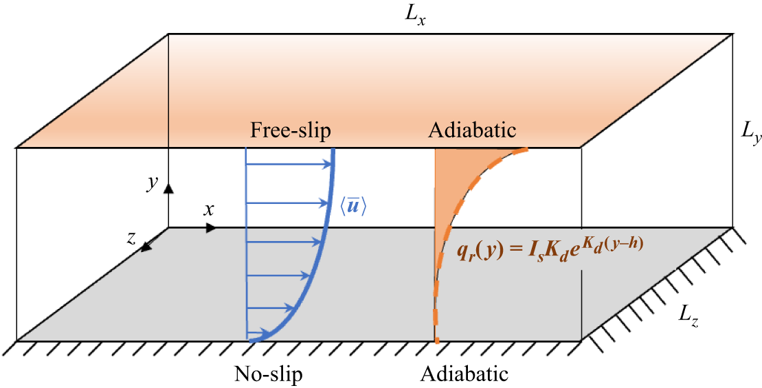
 x
 z
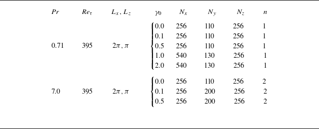
 n
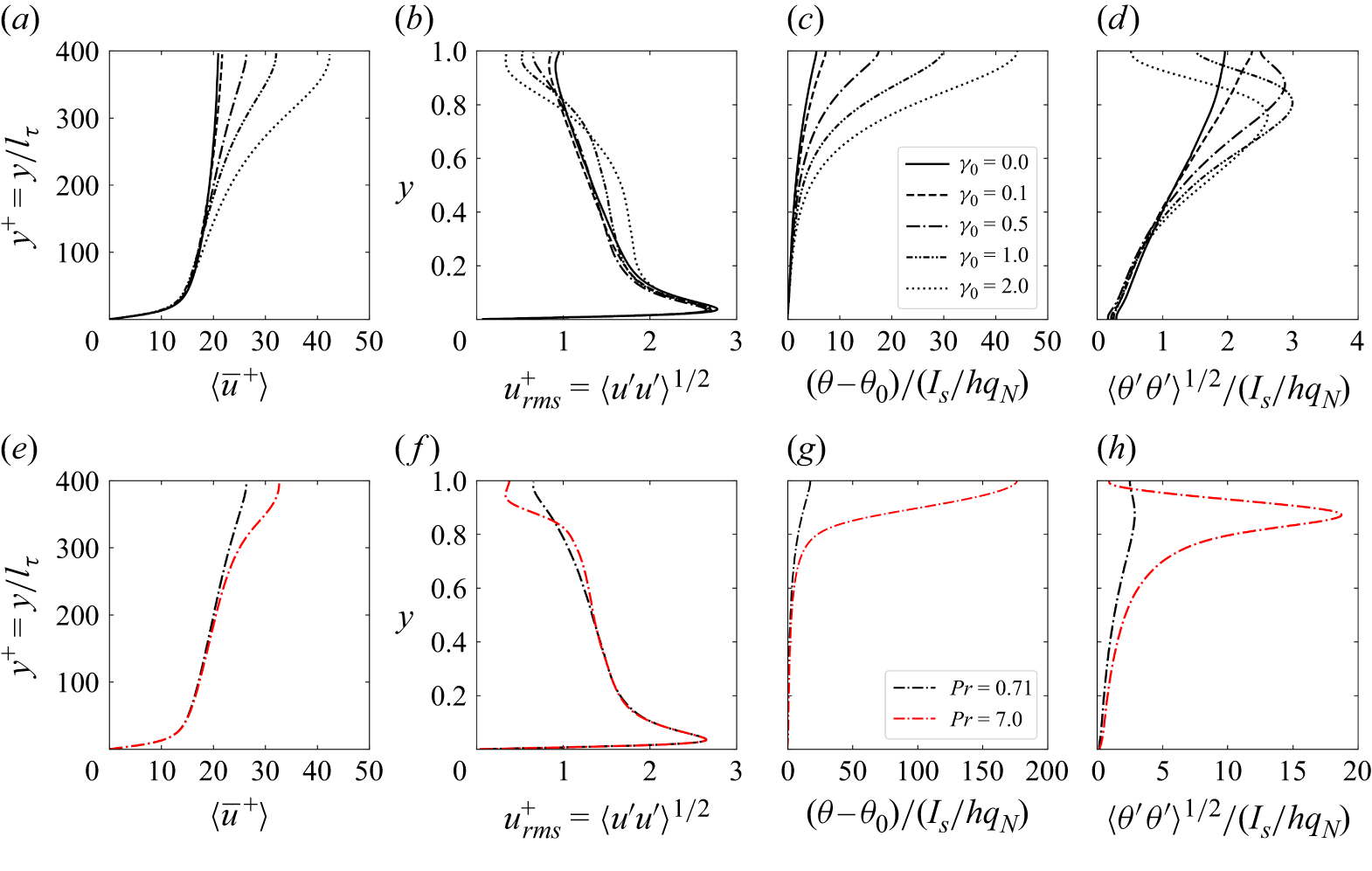
 γ0
 Pr=0.71
 γ0=0.5
 Pr=0.71
 Pr=7

 Pr=0.71
 γ0=0
 γ0=0.1
 γ0=0.5
 γ0=1
 γ0=2
 (Euu,γ0−Euu,0)
 lO+

 Pr=7
 γ0=0
 γ0=0.1
 γ0=0.5
 (Euu,γ0−Euu,0)
 lO+

 γ0
 y+=15
 y=0.5
 y=0.7
 y=0.9
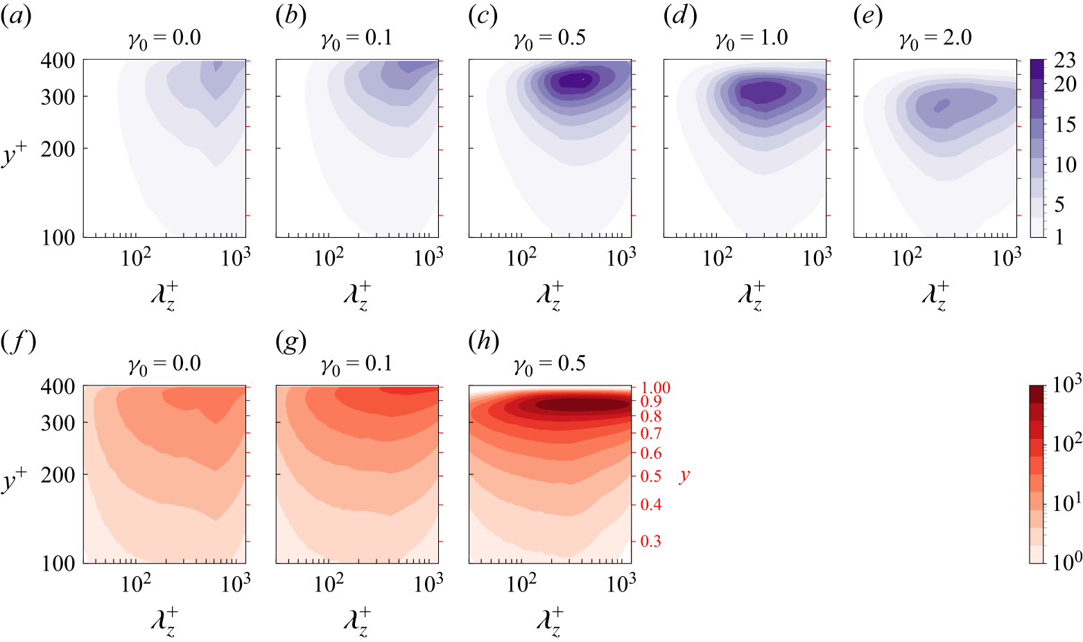
 Pr=0.71
 Pr=7
 γ0=0
 γ0=0.1
 γ0=0.5
 γ0=1
 γ0=2
 log10
 1
 103

 γ0
 y+=15
 y=0.5
 y=0.7
 y=0.9
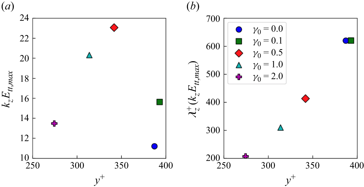
 γ0
 Pr=0.71

 Pr=0.71
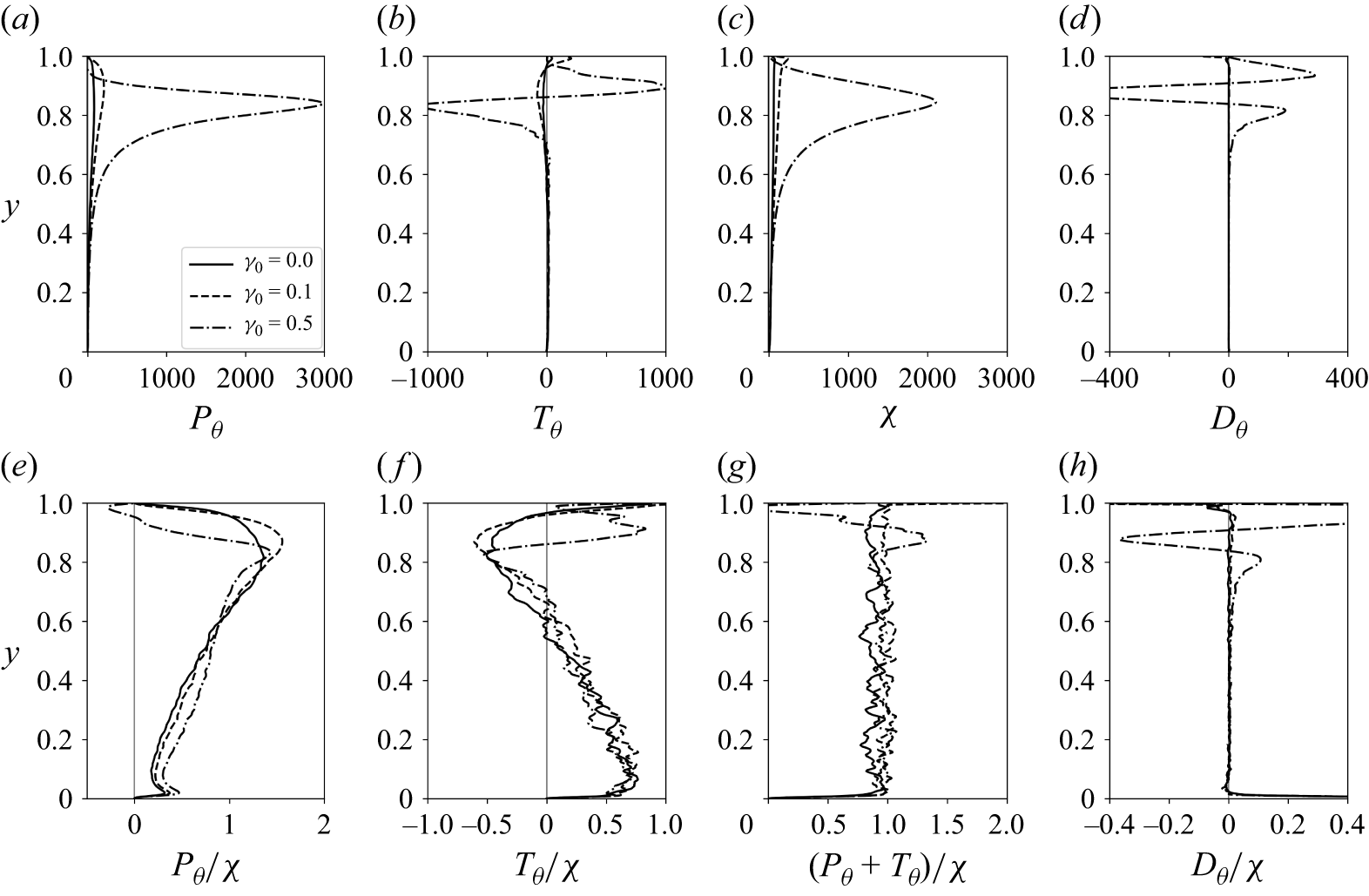
 Pr=7

 Pr=0.71
 γ0=0
 Ruu
 Rvv
 Rww
 99
 y+=20

 γ0
 Pr
 γ0=1
 y⩾0.8
 γ0=2
 y⩾0.3
 Λuu

 u′
 γ0=1
 γ0=2

 Pr=0.71
 u′
 v′
 w′
 θ′

 Pr=7
 u′
 v′
 w′
 θ′
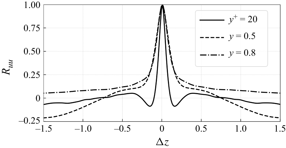
 Ruu
 Pr=0.71
 γ0=2
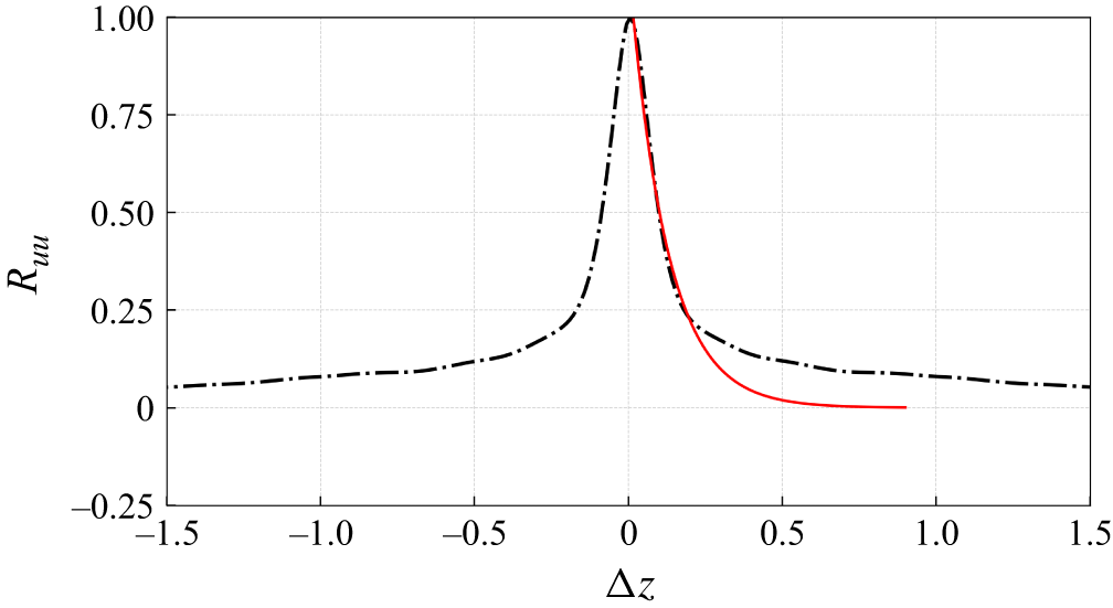
 Ruu
 y=0.8
 Pr=0.71
 γ0=2

 ηK
 lO
 γ0
 Pr=0.71
 Pr=7
 ηK
 lO

 Δy
 ηK
 ηB
 lO
 γ0
 Pr=0.71
 Pr=7

 Pr=0.71
 γ0=0
 γ0=0.1
 γ0=0.5
 γ0=1
 γ0=2
 (Euu,γ0(kx)−Euu,0(kx))

 Pr=7
 γ0=0
 γ0=0.1
 γ0=0.5
 (Euu,γ0(kx)−Euu,0(kx))

 Open access

