2.1. Representation

We look for a representation of the body as the single layer, namely the surface distribution of sources and sinks,

(2.3)\begin{equation} q(\boldsymbol{x}) = \boldsymbol{\nabla}\boldsymbol{\cdot}\boldsymbol{u} = \sigma(\boldsymbol{x})\delta_S(\boldsymbol{x}), \end{equation}

with $\delta _S$ the Dirac delta function of support $S$. This distribution appears as a source term on the right-hand side of (2.1) and generates the potential

(2.4)\begin{equation} \phi(\boldsymbol{x}) ={-}\frac{1}{4{\rm \pi}} \int_S \frac{\sigma(\boldsymbol{x}')}{|\boldsymbol{x}-\boldsymbol{x}'|} \,\mathrm{d}^2S'. \end{equation}

The boundary condition is turned into an integro-differential equation

(2.5)\begin{equation} U_n(\boldsymbol{x}) ={-}\frac{1}{4{\rm \pi}} \frac{\partial}{\partial n} \int_S \frac{\sigma(\boldsymbol{x}')}{|\boldsymbol{x}-\boldsymbol{x}'|} \,\mathrm{d}^2S' \quad (\boldsymbol{x} \in S_+), \end{equation}

to be solved for the layer density $\sigma$ given the normal velocity $U_n$.

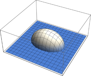
The body is taken to be a triaxial ellipsoid of semi-axes $a > b > c$, represented in figure 1, with

(2.6)\begin{equation} \frac{x^2}{a^2}+\frac{y^2}{b^2}+\frac{z^2}{c^2} = 1 \end{equation}

in Cartesian coordinates $(x,y,z)$. We introduce the ellipsoidal coordinates $(\rho,\mu,\nu )$, defined in (A3). The ellipsoid becomes the surface $\rho = a$, and the boundary condition becomes

(2.7) \begin{align} U_n(\mu,\nu) ={-}\frac{bc}{4{\rm \pi}} \frac{\partial}{\partial\rho} \int_{\rho'=a} \frac{\sigma(\mu',\nu')}{|\boldsymbol{x}-\boldsymbol{x}'|} \frac{(a^2-\mu'^2)^{1/2}(a^2-\nu'^2)^{1/2}}{(a^2-\mu^2)^{1/2}(a^2-\nu^2)^{1/2}} \,\mathrm{d}\varpi' \quad (\rho = a+0), \end{align}

with $\mathrm {d}\varpi$ the solid angle element (A8). Further introduction of the eccentric angles $(\vartheta,\varphi )$, related to $(\mu,\nu )$ by (A9), parametrizes the ellipsoid as

(2.8a–c) \begin{equation} x = a\cos\vartheta, \quad y = b\sin\vartheta\cos\varphi, \quad z = c\sin\vartheta\sin\varphi, \end{equation}

with $0 < \vartheta < {\rm \pi}$ and $0 < \varphi < 2{\rm \pi}$, transferring the integration onto the unit sphere, with solid angle element $\mathrm {d}\varpi = \sin \vartheta \,\mathrm {d}\vartheta \,\mathrm {d}\varphi$. The boundary condition becomes

(2.9)\begin{equation} U_n(\mu,\nu) ={-}\frac{bc}{4{\rm \pi}} \frac{\partial}{\partial\rho} \int_0^{2{\rm \pi}}\!\!\! \int_0^{\rm \pi} \frac{\sigma(\mu',\nu')}{|\boldsymbol{x}-\boldsymbol{x}'|} \frac{(a^2-\mu'^2)^{1/2}(a^2-\nu'^2)^{1/2}}{(a^2-\mu^2)^{1/2}(a^2-\nu^2)^{1/2}} \sin\vartheta' \,\mathrm{d}\vartheta' \,\mathrm{d}\varphi', \end{equation}

where $\rho ' = a$ and $\rho = a+0$.

Figure 1.

Ellipsoid of aspect ratios $\epsilon _1 = c/b = 1/2$ and $\epsilon _3 = b/a = 2/3$.

The problem is solved in ellipsoidal harmonics, combining the Lamé functions $E_l^m(\rho )$, the elliptic integrals $I_l^m(\rho )$ and the surface harmonics $s_l^m(\vartheta,\varphi )$, presented in §§ A.2 and A.3, with the degree $l$ taking the values $0,1,2,\ldots$ and the index $m$ the values $1,2,\ldots,2l+1$. The known $U_n(\mu,\nu )$ is expanded as

(2.10)\begin{equation} (a^2-\mu^2)^{1/2}(a^2-\nu^2)^{1/2} U_n(\mu,\nu) = \sum_{l=0}^\infty\sum_{m=1}^{2l+1} U_{lm}s_l^m(\vartheta,\varphi), \end{equation}

and the unknown $\sigma (\mu,\nu )$ as

(2.11)\begin{equation} (a^2-\mu^2)^{1/2}(a^2-\nu^2)^{1/2} \sigma(\mu,\nu) = \sum_{l=0}^\infty\sum_{m=1}^{2l+1} \sigma_{lm}s_l^m(\vartheta,\varphi). \end{equation}

Expansion (A37) of the kernel $1/|\boldsymbol {x}-\boldsymbol {x}'|$ yields, for $\rho ' = a$ and $\rho = a+0$,

(2.12)\begin{equation} \frac{\partial}{\partial\rho} \frac{1}{|\boldsymbol{x}-\boldsymbol{x}'|} ={-}\frac{4{\rm \pi}}{bc} \sum_{l = 0}^\infty \sum_{m = 1}^{2l+1} [1-bcE_l^m(a)E_l^{m\,\prime}(a)I_l^m(a)] s_l^m(\vartheta,\varphi)s_l^m(\vartheta',\varphi'). \end{equation}

In view of the orthonormality relation (A31), we obtain

(2.13)\begin{equation} \sigma_{lm} = \frac{U_{lm}}{1-bcE_l^m(a)E_l^{m\,\prime}(a)I_l^m(a)}, \end{equation}

and the representation of the ellipsoid follows as

(2.14)\begin{equation} q(\boldsymbol{x}) = \frac{1}{abc} \delta\left[\left(\frac{x^2}{a^2}+\frac{y^2}{b^2}+\frac{z^2}{c^2}\right)^{1/2}-1\right] \sum_{l=0}^\infty\sum_{m=1}^{2l+1} \sigma_{lm}s_l^m(\vartheta,\varphi), \end{equation}

with $\delta$ the Dirac delta function.

2.2. Spectrum

The spectrum

(2.15)\begin{equation} q(\boldsymbol{k}) = \int_S\sigma(\boldsymbol{x})\exp(-\mathrm{i}\boldsymbol{k}\boldsymbol{\cdot}\boldsymbol{x})\,\mathrm{d}^2S \end{equation}

is also of interest, with later application to waves in mind. We note for now that the source and dipole strengths

(2.16a,b)\begin{equation} {\mathcal{S}} = \int_S\sigma(\boldsymbol{x})\,\mathrm{d}^2S, \quad \boldsymbol{{\mathcal{D}}} = \int_S\boldsymbol{x}\sigma(\boldsymbol{x})\,\mathrm{d}^2S, \end{equation}

respectively, may be deduced from the small-wavenumber expansion

(2.17)\begin{equation} q(\boldsymbol{k}) \sim {\mathcal{S}}-\mathrm{i}\boldsymbol{k}\boldsymbol{\cdot}\boldsymbol{{\mathcal{D}}}. \end{equation}

We thus need to calculate the integral

(2.18)\begin{equation} q(\boldsymbol{k}) = \sum_{l=0}^\infty \sum_{m=1}^{2l+1} \sigma_{lm} \int_0^{2{\rm \pi}}\!\!\! \int_0^{\rm \pi} \exp(-\mathrm{i}\boldsymbol{k}\boldsymbol{\cdot}\boldsymbol{x}) s_l^m(\vartheta,\varphi) \sin\vartheta \,\mathrm{d}\vartheta \,\mathrm{d}\varphi, \end{equation}

where $\boldsymbol {x}$ is related to $(\vartheta,\varphi )$ by (2.8).

In spherical geometry, the natural basis for expanding a function of the spherical angles $(\vartheta,\varphi )$ is the surface harmonics

(2.19)\begin{equation} Y_l^n(\vartheta,\varphi) = \sqrt{\frac{2l+1}{4{\rm \pi}}\frac{(l-n)!}{(l+n)!}} \operatorname{P}_l^n(\cos\vartheta)\exp(\mathrm{i}n\varphi), \end{equation}

with $\operatorname {P}_l^n$ an associated Legendre function, of degree $l = 0,1,2,\ldots$ and order $n = -l,-l+1,\ldots,l-1,l$. See for example Jackson (Reference Jackson1999, § 3.5). Then, Gegenbauer's finite integral

(2.20) \begin{align} \int_0^{\rm \pi}\exp(\mathrm{i}\kappa\cos\vartheta\cos\vartheta_k)\operatorname{J}_n(\kappa\sin\vartheta\sin\vartheta_k) \operatorname{P}_l^n(\cos\vartheta)\sin\vartheta\,\mathrm{d}\vartheta = 2\mathrm{i}^{l-n}\operatorname{j}_l(\kappa)\operatorname{P}_l^n(\cos\vartheta_k), \end{align}

derived by Watson (Reference Watson1944, § 12.14), where $\operatorname {J}_n$ denotes a cylindrical Bessel function and $\operatorname {j}_l$ a spherical Bessel function, leads to the Funk–Hecke formula

(2.21)\begin{equation} \int_0^{2{\rm \pi}} \!\!\!\int_0^{\rm \pi} \exp(-\mathrm{i}\boldsymbol{k}\boldsymbol{\cdot}\boldsymbol{x}) Y_l^n(\vartheta,\varphi) \sin\vartheta\,\mathrm{d}\vartheta \,\mathrm{d}\varphi = 4{\rm \pi}(-\mathrm{i})^l \operatorname{j}_l(\kappa) Y_l^n(\vartheta_k,\varphi_k), \end{equation}

with $(\vartheta _k,\varphi _k)$ the spherical angles in Fourier space, such that

(2.22)\begin{equation} \boldsymbol{k}\boldsymbol{\cdot}\boldsymbol{x} = \kappa [\cos\vartheta\cos\vartheta_k+\sin\vartheta\sin\vartheta_k\cos(\varphi-\varphi_k)]. \end{equation}

See for example Martin (Reference Martin2006, § 3.6).

In ellipsoidal geometry, Hobson (Reference Hobson1931, §§ 280–281) pointed out that each surface spherical harmonic $Y_l^n(\vartheta,\varphi )$, with $(\vartheta,\varphi )$ the eccentric angles, is a linear combination of the $2l+1$ ellipsoidal harmonics $s_l^m(\vartheta,\varphi )$ of the same degree $l$. Conversely, each surface ellipsoidal harmonic $s_l^m(\vartheta,\varphi )$ is a linear combination of the spherical harmonics $Y_l^n(\vartheta,\varphi )$ of the same degree. Accordingly, the Funk–Hecke formula generalizes to ellipsoidal harmonics in the form

(2.23)\begin{equation} \int_0^{2{\rm \pi}} \!\!\! \int_0^{\rm \pi} \exp(-\mathrm{i}\boldsymbol{k}\boldsymbol{\cdot}\boldsymbol{x}) s_l^m(\vartheta,\varphi) \sin\vartheta\,\mathrm{d}\vartheta \,\mathrm{d}\varphi = 4{\rm \pi}(-\mathrm{i})^l \operatorname{j}_l(\kappa) s_l^m(\vartheta_k,\varphi_k), \end{equation}

where the angles $(\vartheta _k,\varphi _k)$ are defined in Fourier space by

(2.24a–c)\begin{equation} k_xa = \kappa\cos\vartheta_k, \quad k_yb = \kappa\sin\vartheta_k\cos\varphi_k, \quad k_zc = \kappa\sin\vartheta_k\sin\varphi_k, \end{equation}

with $\kappa = (k_x^2a^2+k_y^2b^2+k_z^2c^2)^{1/2}$.

We thus have

(2.25)\begin{equation} q(\boldsymbol{k}) = 4{\rm \pi} \sum_{l=0}^\infty (-\mathrm{i})^l \operatorname{j}_l[(k_x^2a^2+k_y^2b^2+k_z^2c^2)^{1/2}] \sum_{m=1}^{2l+1} \sigma_{lm} s_l^m(\vartheta_k,\varphi_k), \end{equation}

generalizing Voisin (Reference Voisin2021, (6.28)), obtained for a spheroid.

2.3. Monopolar motion

The analysis is applied first to the radial expansion or contraction of the ellipsoid at the velocity $\boldsymbol {U} = U\boldsymbol {x}/(abc)^{1/3}$, with $U$ a constant. Such forcing is of degree $l = 0$, with

(2.26)\begin{equation} U_{01} = \sqrt{4{\rm \pi}}U (abc)^{2/3} = \sigma_{01}. \end{equation}

It has the representation

(2.27)\begin{equation} q(\boldsymbol{x}) = \frac{U}{(abc)^{1/3}} \delta\left[\left(\frac{x^2}{a^2}+\frac{y^2}{b^2}+\frac{z^2}{c^2}\right)^{1/2}-1\right] \end{equation}

and the spectrum

(2.28)\begin{equation} q(\boldsymbol{k}) = 4{\rm \pi} U(abc)^{2/3} \operatorname{j}_0[(k_x^2a^2+k_y^2b^2+k_z^2c^2)^{1/2}], \end{equation}

corresponding to a source of strength ${\mathcal {S}} = 4{\rm \pi} U(abc)^{2/3}$.

2.4. Dipolar motion

The translation of a rigid ellipsoid at the velocity $\boldsymbol {U} = U\boldsymbol {e}_x+V\boldsymbol {e}_y+W\boldsymbol {e}_z$, with $(U,V,W)$ constants, is of degree $l = 1$, such that

(2.29a–c)\begin{equation} U_{11} = \sqrt{\frac{4{\rm \pi}}{3}}bcU, \quad U_{12} = \sqrt{\frac{4{\rm \pi}}{3}}acV, \quad U_{13} = \sqrt{\frac{4{\rm \pi}}{3}}abW. \end{equation}

The equivalent source has coefficients

(2.30a–c)\begin{equation} \sigma_{11} = \frac{U_{11}}{1-A}, \quad \sigma_{12} = \frac{U_{12}}{1-B}, \quad \sigma_{13} = \frac{U_{13}}{1-C}, \end{equation}

where $A$, $B$ and $C$ are related to the Legendre integrals (A18) by

(2.31a)$$\begin{gather} A = abcI_1^1(a) = \frac{abc}{a^2-b^2} \frac{F(\alpha,\beta)-E(\alpha,\beta)}{(a^2-c^2)^{1/2}}, \end{gather}$$

(2.31b)$$\begin{gather}B = abcI_1^2(a) = \frac{abc}{a^2-b^2} \frac{E(\alpha,\beta)/(1-\beta)-F(\alpha,\beta)}{(a^2-c^2)^{1/2}} - \frac{c^2}{b^2-c^2}, \end{gather}$$

(2.31c)$$\begin{gather}C = abcI_1^3(a) = \frac{b^2}{b^2-c^2}- \frac{abc}{b^2-c^2}\frac{E(\alpha,\beta)}{(a^2-c^2)^{1/2}}, \end{gather}$$

with

(2.32a,b)\begin{equation} \alpha = \arccos\left(\frac{c}{a}\right), \quad \beta = \frac{a^2-b^2}{a^2-c^2}. \end{equation}

These $A$, $B$ and $C$ are identical to $\alpha _0/2$, $\beta _0/2$ and $\gamma _0/2$, respectively, in Lamb (Reference Lamb1932, § 114) and Milne-Thomson (Reference Milne-Thomson1968, § 17.52), and $A_0/2$, $B_0/2$ and $C_0/2$ in Kochin, Kibel’ & Roze (Reference Kochin, Kibel’ and Roze1964, §§ 7.2 and 7.8) and Korotkin (Reference Korotkin2009, § 3.1), all expressed as gravitational potentials. See also Dassios (Reference Dassios2012, § 13.5).

Forcing is of the dipolar type, in direct space

(2.33)\begin{equation} q(\boldsymbol{x}) = \left( \frac{U}{1-A}\frac{x}{a^2}+\frac{V}{1-B}\frac{y}{b^2}+\frac{W}{1-C}\frac{z}{c^2} \right) \delta\left[\left(\frac{x^2}{a^2}+\frac{y^2}{b^2}+\frac{z^2}{c^2}\right)^{1/2}-1\right], \end{equation}

and in Fourier space

(2.34)\begin{equation} q(\boldsymbol{k}) ={-}4\mathrm{i}{\rm \pi} abc \left( \frac{Uk_x}{1-A}+\frac{Vk_y}{1-B}+\frac{Wk_z}{1-C} \right) \frac{\operatorname{j}_1[(k_x^2a^2+k_y^2b^2+k_z^2c^2)^{1/2}]}{(k_x^2a^2+k_y^2b^2+k_z^2c^2)^{1/2}}, \end{equation}

with strength

(2.35)\begin{equation} \boldsymbol{{\mathcal{D}}} = \frac{4}{3}{\rm \pi} abc \left( \frac{U}{1-A}\boldsymbol{e}_x+\frac{V}{1-B}\boldsymbol{e}_y+\frac{W}{1-C}\boldsymbol{e}_z \right). \end{equation}

The bodies considered by Voisin (Reference Voisin2021, Reference Voisin2024) are recovered as particular cases. These include: the oblate spheroid, for which

(2.36a,b)\begin{equation} A = B = \frac{1-D(\epsilon)}{2}, \quad C = D(\epsilon) = \frac{1}{1-\epsilon^2} \left[1-\frac{\epsilon\arccos\epsilon}{(1-\epsilon^2)^{1/2}}\right], \end{equation}

where $\epsilon = c/a < 1$, corresponding to $a = b$, namely $\beta \to 0$; the prolate spheroid, for which

(2.37a,b)\begin{equation} A = D(\epsilon) = \frac{1}{1-\epsilon^2} \left[1-\frac{\epsilon\,{\rm arccosh}\,\epsilon}{(\epsilon^2-1)^{1/2}}\right], \quad B = C = \frac{1-D(\epsilon)}{2}, \end{equation}

where $\epsilon = a/b > 1$, corresponding to $b = c$, namely $\beta \to 1$; and the elliptic cylinder, for which

(2.38a–c)\begin{equation} A = 0, \quad B = \frac{\epsilon}{1+\epsilon}, \quad C = \frac{1}{1+\epsilon}, \end{equation}

where $\epsilon = c/b < 1$, corresponding to $a \to \infty$, namely $(\alpha,\beta ) \to ({\rm \pi} /2,1)$. More specific cases are the sphere, for which

(2.39)\begin{equation} A = B = C = \tfrac{1}{3}, \end{equation}

corresponding to $a = b = c$, and the circular cylinder, for which

(2.40a,b)\begin{equation} A = 0, \quad B = C = \tfrac{1}{2}, \end{equation}

corresponding to $a \to \infty$ and $b = c$.

2.5. Added mass

The dynamics of a rigid body in an inviscid fluid is governed by its added mass, representing the additional inertia imparted to it by the motion of the fluid (Batchelor Reference Batchelor1967, § 6.4; Lighthill Reference Lighthill1986, § 8.3; Landau & Lifshitz Reference Landau and Lifshitz1987, § 11). The added mass tensor of the ellipsoid is diagonal, and the ratios $C_x$, $C_y$ and $C_z$ of its elements to the mass of the displaced fluid are related to the components ${\mathcal {D}}_x$, ${\mathcal {D}}_y$ and ${\mathcal {D}}_z$ of the dipole strength by

(2.41a–c)\begin{equation} C_x = \frac{{\mathcal{D}}_x}{{\mathcal{V}}U}-1, \quad C_y = \frac{{\mathcal{D}}_y}{{\mathcal{V}}V}-1, \quad C_z = \frac{{\mathcal{D}}_z}{{\mathcal{V}}W}-1, \end{equation}

with ${\mathcal {V}} = (4/3){\rm \pi} abc$ the volume of the ellipsoid. We obtain

(2.42a–c)\begin{equation} C_x = \frac{A}{1-A}, \quad C_y = \frac{B}{1-B}, \quad C_z = \frac{C}{1-C}. \end{equation}

Introducing the aspect ratios $\epsilon _1 = c/b$ and $\epsilon _3 = b/a$, both smaller than $1$, we have

(2.43a)$$\begin{gather} A(\epsilon_1,\epsilon_3) = \frac{\epsilon_1\epsilon_3^2}{1-\epsilon_3^2} \frac{F(\alpha,\beta)-E(\alpha,\beta)}{(1-\epsilon_1^2\epsilon_3^2)^{1/2}}, \end{gather}$$

(2.43b)$$\begin{gather}B(\epsilon_1,\epsilon_3) = \frac{\epsilon_1\epsilon_3^2}{1-\epsilon_3^2} \frac{E(\alpha,\beta)/(1-\beta)-F(\alpha,\beta)}{(1-\epsilon_1^2\epsilon_3^2)^{1/2}} - \frac{\epsilon_1^2}{1-\epsilon_1^2}, \end{gather}$$

(2.43c)$$\begin{gather}C(\epsilon_1,\epsilon_3) = \frac{1}{1-\epsilon_1^2}- \frac{\epsilon_1}{1-\epsilon_1^2}\frac{E(\alpha,\beta)}{(1-\epsilon_1^2\epsilon_3^2)^{1/2}}, \end{gather}$$

where

(2.44a,b)\begin{equation} \alpha = \arccos(\epsilon_1\epsilon_3), \quad \beta = \frac{1-\epsilon_3^2}{1-\epsilon_1^2\epsilon_3^2}. \end{equation}

The variations of the added mass coefficients with $\epsilon _1$ and $\epsilon _3$ are plotted in figure 2. They are in agreement with figures 150–152 of Kochin et al. (Reference Kochin, Kibel’ and Roze1964) and 3.1–3.2 of Korotkin (Reference Korotkin2009), representing the variations of the coefficients with $\epsilon _1$ for specific values of $1/\epsilon _3$.

Figure 2.

Added mass coefficients for the translation of an ellipsoid of semi-axes $a > b > c$ along the associated directions (a) $x$, (b) $y$ and (c) $z$ in a homogeneous fluid. The coefficients are determined by the aspect ratios $\epsilon _1 = c/b$ and $\epsilon _3 = b/a$.

3.1. Representation

The single layer (2.3) generates the potential

(3.3)\begin{equation} \psi(\boldsymbol{x}) = \frac{1}{4{\rm \pi}(\omega^2-N^2)^{1/2}} \int_S \frac{\sigma(\boldsymbol{x}')\,\mathrm{d}^2S'}{[(\omega^2(\boldsymbol{x}-\boldsymbol{x}')^2-N^2(z-z')^2]^{1/2}}, \end{equation}

where the determination of the square roots is set by cuts, extending vertically downwards away from the branch points $\pm N$ and $\pm N|z-z'|/|\boldsymbol {x}-\boldsymbol {x}'|$ in the $\omega$-plane. The boundary condition becomes

(3.4)\begin{align} U_n(\boldsymbol{x}) &= \frac{1}{4{\rm \pi}(\omega^2-N^2)^{1/2}} \left( N^2\frac{\partial}{\partial n_{\mathrm{h}}}- \omega^2\frac{\partial}{\partial n} \right) \nonumber\\ &\quad \times \int_S \frac{\sigma(\boldsymbol{x}')\,\mathrm{d}^2S'}{[(\omega^2(\boldsymbol{x}-\boldsymbol{x}')^2-N^2(z-z')^2]^{1/2}} \quad (\boldsymbol{x} \in S_+). \end{align}

We follow the approach introduced by Bryan (Reference Bryan1889) for inertial waves, Pierce (Reference Pierce1963) for acoustic-gravity waves and Hurley (Reference Hurley1972) for internal waves; namely, we consider real evanescent frequencies $\omega > N$ first, stretching the coordinates anisotropically so as to transform the wave equation into the Laplace equation, then we continue the solution analytically to the upper half of the complex $\omega$-plane.

The coordinates are stretched according to

(3.5a–c)\begin{equation} x_\star = \frac{\omega}{N}x, \quad y_\star = \frac{\omega}{N}y, \quad z_\star = \left(\frac{\omega^2}{N^2}-1\right)^{1/2}z. \end{equation}

This transforms the boundary condition into

(3.6)\begin{equation} U_n(\boldsymbol{x}) = \frac{1}{4{\rm \pi} N(\omega^2-N^2)^{1/2}} \left( N^2\frac{\partial}{\partial n_{\mathrm{h}}}- \omega^2\frac{\partial}{\partial n} \right) \int_S \frac{\sigma(\boldsymbol{x}')}{|\boldsymbol{x}_\star -\boldsymbol{x}'_\star|} \,\mathrm{d}^2S' \quad (\boldsymbol{x} \in S_+), \end{equation}

and the ellipsoid (2.6) into another, with semi-axes

(3.7a–c)\begin{equation} a_\star = \frac{\omega}{N}a, \quad b_\star = \frac{\omega}{N}b, \quad c_\star = \left(\frac{\omega^2}{N^2}-1\right)^{1/2}c. \end{equation}

We assume that $a > b > c$, so that $a_\star > b_\star > c_\star$, and we introduce two systems of ellipsoidal coordinates: one $(\rho,\mu,\nu )$ in unstretched space, with semi-axes $(a,b,c)$ and semi-focal distances $(h_1,h_2,h_3)$, such that $\rho = a$ on the ellipsoid; and another $(\rho _\star,\mu _\star,\nu _\star )$ in stretched space, with semi-axes $(a_\star,b_\star,c_\star )$ and semi-focal distances $(h_{1_\star },h_{2_\star },h_{3_\star })$, such that $\rho _\star = a_\star$ on the ellipsoid. The boundary condition becomes

(3.8) \begin{align} U_n(\mu,\nu) ={-}\frac{b_\star c_\star}{4{\rm \pi}} \frac{\partial}{\partial\rho_\star} \int_{\rho'=a} \frac{\sigma(\mu',\nu')}{|\boldsymbol{x}_\star -\boldsymbol{x}'_\star|} \frac{(a^2-\mu'^2)^{1/2}(a^2-\nu'^2)^{1/2}}{(a^2-\mu^2)^{1/2}(a^2-\nu^2)^{1/2}} \,\mathrm{d}\varpi' \quad (\rho = a+0). \end{align}

The difficulty lies in the fact that differentiation is performed in stretched coordinates, while integration is performed in unstretched coordinates.

However, even though the coordinates $(\mu,\nu )$ and $(\mu _\star,\nu _\star )$ are distinct on the ellipsoid, the eccentric angles $(\vartheta,\varphi )$ are not, since

(3.9a–c)\begin{equation} \frac{x}{a} = \frac{x_\star}{a_\star} = \cos\vartheta, \quad \frac{y}{b} = \frac{y_\star}{b_\star} = \sin\vartheta\cos\varphi, \quad \frac{z}{c} = \frac{z_\star}{c_\star} = \sin\vartheta\sin\varphi, \end{equation}

with two consequences. First, the boundary condition becomes

(3.10) \begin{align} U_n(\mu,\nu) ={-}\frac{b_\star c_\star}{4{\rm \pi}} \frac{\partial}{\partial\rho_\star} \int_0^{2{\rm \pi}} \!\!\! \int_0^{\rm \pi} \frac{\sigma(\mu',\nu')}{|\boldsymbol{x}_\star - \boldsymbol{x}'_\star|} \frac{(a^2-\mu'^2)^{1/2}(a^2-\nu'^2)^{1/2}}{(a^2-\mu^2)^{1/2}(a^2-\nu^2)^{1/2}} \sin\vartheta' \,\mathrm{d}\vartheta' \,\mathrm{d}\varphi', \end{align}

where $\rho '_\star = a_\star$ and $\rho _\star = a_\star +0$. Second, the same surface harmonics $s_l^m(\vartheta,\varphi )$ are involved, on the one hand in the expansions (2.10) and (2.11) of $U_n(\mu,\nu )$ and $\sigma (\mu,\nu )$, respectively, and on the other hand in the expansion of $1/|\boldsymbol {x}_\star -\boldsymbol {x}'_\star |$, yielding, for $\rho '_\star = a_\star$ and $\rho _\star = a_\star +0$,

(3.11) \begin{align} \frac{\partial}{\partial\rho_\star} \frac{1}{|\boldsymbol{x}_\star -\boldsymbol{x}'_\star|} ={-}\frac{4{\rm \pi}}{b_\star c_\star} \sum_{l = 0}^\infty \sum_{m = 1}^{2l+1} [1-b_\star c_\star E_l^m(a_\star)E_l^{m\,\prime}(a_\star)I_l^m(a_\star)] s_l^m(\vartheta,\varphi)s_l^m(\vartheta',\varphi'). \end{align}

Accordingly, the only change in the results of §§ 2.1 and 2.2 is the replacement of $a$, $b$ and $c$ by $a_\star$, $b_\star$ and $c_\star$ in the relation between $\sigma _{lm}$ and $U_{lm}$, consistent with the rule of affine similitude put forward by Ermanyuk (Reference Ermanyuk2002). We obtain

(3.12)\begin{equation} \sigma_{lm} = \frac{U_{lm}}{1-b_\star c_\star E_l^m(a_\star)E_l^{m\,\prime}(a_\star)I_l^m(a_\star)}. \end{equation}

Analytic continuation to the upper half of the $\omega$-plane allows the extension of this solution to other values of $\omega$ and other orderings of $a$, $b$ and $c$.

3.2. Dipolar oscillations

Monopolar oscillations are unaffected by the stratification, but dipolar oscillations are. The relevant geometrical parameters are the horizontal aspect ratio $\epsilon _{h} = b/a$ and the vertical aspect ratio $\epsilon _{v} = c/b$, and the relevant physical parameter is the frequency ratio $\varOmega = \omega /N$. We introduce

(3.13)\begin{equation} \varUpsilon_{v} = \frac{c_\star}{b_\star} = \epsilon_{v}\left(1-\frac{1}{\varOmega^2}\right)^{1/2}, \end{equation}

generalizing the notation $\varUpsilon$ of Voisin (Reference Voisin2021, Reference Voisin2024). Equations (2.33)–(2.35) for the equivalent source and dipole strength remain valid, with

(3.14a)$$\begin{gather} A(\varUpsilon_{v},\epsilon_{h}) = \frac{\epsilon_{h}^2\varUpsilon_{v}}{1-\epsilon_{h}^2} \frac{F(\alpha,\beta)-E(\alpha,\beta)}{(1-\epsilon_{h}^2\varUpsilon_{v}^2)^{1/2}}, \end{gather}$$

(3.14b)$$\begin{gather}B(\varUpsilon_{v},\epsilon_{h}) = \frac{\epsilon_{h}^2\varUpsilon_{v}}{1-\epsilon_{h}^2} \frac{E(\alpha,\beta)/(1-\beta)-F(\alpha,\beta)}{(1-\epsilon_{h}^2\varUpsilon_{v}^2)^{1/2}} - \frac{\varUpsilon_{v}^2}{1-\varUpsilon_{v}^2}, \end{gather}$$

(3.14c)$$\begin{gather}C(\varUpsilon_{v},\epsilon_{h}) = \frac{1}{1-\varUpsilon_{v}^2}- \frac{\varUpsilon_{v}}{1-\varUpsilon_{v}^2} \frac{E(\alpha,\beta)}{(1-\epsilon_{h}^2\varUpsilon_{v}^2)^{1/2}}, \end{gather}$$

where

(3.15a,b)\begin{equation} \alpha = \arccos(\epsilon_{h}\varUpsilon_{v}), \quad \beta = \frac{1-\epsilon_{h}^2}{1-\epsilon_{h}^2\varUpsilon_{v}^2}. \end{equation}

The limit $\epsilon _{h} \to 1$ corresponds to a spheroid of vertical $z$-axis and gives

(3.16a,b)\begin{equation} A = B = \frac{1-D(\varUpsilon_{v})}{2}, \quad C = D(\varUpsilon_{v}) = \frac{1}{1-\varUpsilon_{v}^2} \left[1-\frac{\varUpsilon_{v}\arccos\varUpsilon_{v}}{(1-\varUpsilon_{v}^2)^{1/2}}\right], \end{equation}

while the limit $\epsilon _{h} \to 0$ corresponds to an elliptic cylinder of horizontal $x$-axis and gives

(3.17a–c)\begin{equation} A = 0, \quad B = \frac{\varUpsilon_{v}}{1+\varUpsilon_{v}}, \quad C = \frac{1}{1+\varUpsilon_{v}}. \end{equation}

Both limits are consistent with Voisin (Reference Voisin2021, Reference Voisin2024).

3.3. Added mass

In the presence of density stratification, the added mass coefficients vary with the frequency. For a body having the horizontal $x$- and $y$-axes and the vertical $z$-axis as principal directions, the coefficients have been shown by Ermanyuk (Reference Ermanyuk2002) and Voisin (Reference Voisin2024) to be

(3.18a–c) \begin{align} C_x(\omega) = \frac{{\mathcal{D}}_x}{{\mathcal{V}}U}-1, \quad C_y(\omega) = \frac{{\mathcal{D}}_y}{{\mathcal{V}}V}-1, \quad C_z(\omega) = \left(1-\frac{N^2}{\omega^2}\right) \left(\frac{{\mathcal{D}}_z}{{\mathcal{V}}W}-1\right), \end{align}

yielding for the ellipsoid

(3.19a–c)\begin{equation} C_x(\omega) = \frac{A}{1-A}, \quad C_y(\omega) = \frac{B}{1-B}, \quad C_z(\omega) = \left(1-\frac{1}{\varOmega^2}\right)\frac{C}{1-C}. \end{equation}

The variations of these coefficients are plotted in figures 3–5, for several values of $\epsilon _{h}$ and $\epsilon _{v}$ between $1/5$ and $5$. The same trends are observed as for the spheroid of Voisin (Reference Voisin2024), corresponding to $\epsilon _{h} = 1$. For the inertial coefficients, finite values $\epsilon _{h}$ of ${\rm Re}\,C_x(\omega )$ and $1/\epsilon _{h}$ of ${\rm Re}\, C_y(\omega )$ are obtained at $\varOmega = 0$, and a logarithmic divergence of ${\rm Re}\, C_z(\omega )$. The coefficients are zero at $\varOmega = 1$, then they increase towards their values $C_x^\infty$, $C_y^\infty$ and $C_z^\infty$ in the absence of stratification, reached for $\varOmega \to \infty$. The damping coefficients $\varOmega \,{\rm Im}\,C_x(\omega )$, $\varOmega \,{\rm Im} \,C_y(\omega )$ and $\varOmega \,{\rm Im} \,C_z(\omega )$ are zero not only at $\varOmega = 0$ and $1$, but also for all the frequencies $\varOmega > 1$ at which the waves are evanescent.

Figure 3.

Frequency variations of (a,c,e) the inertial coefficient ${\rm Re}\, C_x(\omega )$ and (b,d,f) the damping coefficient $\varOmega \,{\rm Im} \,C_x(\omega )$ of an ellipsoid of horizontal aspect ratio $\epsilon _{h}$ and vertical aspect ratio $\epsilon _{v}$, oscillating along the horizontal $x$-axis in a stratified fluid, for (a,b) $\epsilon _{h} = 0.2$, (c,d) $\epsilon _{h} = 1$ and (e,f) $\epsilon _{h} = 5$.

Figure 4.

Same as figure 3 for oscillations along the horizontal $y$-axis.

Figure 5.

Same as figure 3 for oscillations along the vertical $z$-axis.

A transition is observed, as $\epsilon _{h}$ decreases down to $0$, from the three-dimensional ellipsoid to the two-dimensional elliptic cylinder. As $\epsilon _{h} \to 0$, all three added mass coefficients, once normalized by their values in the absence of stratification, have the same limiting behaviour

(3.20)\begin{equation} \frac{C_x(\omega)}{C_x^\infty} = \frac{C_y(\omega)}{C_y^\infty} = \frac{C_z(\omega)}{C_z^\infty} = \left(1-\frac{1}{\varOmega^2}\right)^{1/2}, \end{equation}

with $C_x^\infty = 0$, $C_y^\infty = \epsilon _{v}$ and $C_z^\infty = 1/\epsilon _{v}$. This behaviour is characterized not only by the absence of wave damping at the evanescent frequencies $\varOmega > 1$, but also by the absence of inertial effects at the propagating frequencies $\varOmega < 1$. The transition is shown in figures 6–8 for several values of $\epsilon _{h}$ between $0$ and $10$. The normalized coefficients undergo little change as $\epsilon _{h}$ increases above $1$.

Figure 6.

Transition to two-dimensionality for (a,c,e,g,i) the inertial coefficients and (b,d,f,h,j) the damping coefficients as $\epsilon _{h}$ decreases down to $0$ for oscillations along the $x$-axis, and (a,b) $\epsilon _{h} = 0$, (c,d) $\epsilon _{h} = 0.01$, (e,f) $\epsilon _{h} = 0.1$, (g,h) $\epsilon _{h} = 1$ and (i,j) $\epsilon _{h} = 10$.

Figure 7.

Same as figure 6 for oscillations along the $y$-axis.

Figure 8.

Same as figure 6 for oscillations along the $z$-axis.

4.1. Impulse response function

When the body moves at the velocity $\boldsymbol {U}(t) = U(t)\boldsymbol {e}_x+V(t)\boldsymbol {e}_y+W(t)\boldsymbol {e}_z$, the fluid exerts on it a hydrodynamic force of $x$-component

(4.1)\begin{equation} F_x(t) ={-}m_{f}C_x^\infty\frac{\mathrm{d}U}{\mathrm{d}t}(t) -m_{f}N \int_0^\infty C_x^{M}(t')\frac{\mathrm{d}U}{\mathrm{d}t}(t-t') \,\mathrm{d}t', \end{equation}

and similarly for the $y$- and $z$-components, with

(4.2)\begin{equation} C_x^{M}(t) = \frac{1}{2{\rm \pi} N} \int [C_x(\omega)-C_x^\infty] \exp(-\mathrm{i}\omega t) \,\mathrm{d}\omega \end{equation}

the impulse response function (Cummins Reference Cummins1962; Ogilvie Reference Ogilvie1964). Accordingly, the force acting on the body combines the same acceleration reaction as in a homogeneous fluid, plus a memory integral representing, in the stratified fluid, the effect of internal wave radiation. As stated by Newman (Reference Newman2017, § 6.19) for surface gravity waves, when the body moves, ‘waves will be generated […]. As time increases, these waves will propagate outward from the body, but they will continue to affect the fluid pressure and hence the body force for all subsequent times. Thus memory effects are introduced.’

Owing to causality, and to the Hermitian property $C_x(-\omega ) = \overline {C_x(\omega )}$, where the overbar denotes a complex conjugate, the impulse response function may be written as

(4.3)\begin{equation} C_x^{M}(t) = \frac{2}{\rm \pi} \frac{H(t)}{N} \int_0^N {\rm Im}[C_x(\omega)] \sin(\omega t) \,\mathrm{d}\omega, \end{equation}

with $H(t)$ the Heaviside step function, and the integral evaluated numerically as, say,

(4.4)\begin{equation} C_x^{M}(t) = \frac{2}{\rm \pi} H(t) \int_0^{{\rm \pi}/2} {\rm Im}[C_x(N\cos\theta)] \sin(Nt\cos\theta) \sin\theta\,\mathrm{d}\theta. \end{equation}

The same applies to $C_y^{M}(t)$ and $C_z^{M}(t)$. The variations of these functions are presented in figure 9, normalized by $C_x^\infty$, $C_y^\infty$ and $C_z^\infty$, with time normalized by the buoyancy period $T = 2{\rm \pi} /N$. As for added mass in figures 6–8, a transition is observed, as $\epsilon _{h} \to 0$, to the response for the elliptic cylinder, identical in all directions and given by

(4.5)\begin{equation} \frac{C_x^{M}(t)}{C_x^\infty} = \frac{C_y^{M}(t)}{C_y^\infty} = \frac{C_z^{M}(t)}{C_z^\infty} = H(t) \int_0^t \operatorname{J}_1(N\tau) \frac{\mathrm{d}\tau}{\tau}, \end{equation}

where

(4.6)\begin{equation} \int_0^t\operatorname{J}_1(N\tau)\frac{\mathrm{d}\tau}{\tau} = Nt\operatorname{J}_0(Nt)\left[1-\frac{\rm \pi}{2}\boldsymbol{H}_1(Nt)\right] -\operatorname{J}_1(Nt)\left[1-\frac{\rm \pi}{2}Nt\boldsymbol{H}_0(Nt)\right], \end{equation}

with $\operatorname {J}_n$ a Bessel function and $\boldsymbol {H}_n$ a Struve function.

Figure 9.

Impulse response functions of an ellipsoid of horizontal aspect ratio (a–c) $\epsilon _{h} = 0$, (d–f) $\epsilon _{h} = 0.01$, (g–i) $\epsilon _{h} = 0.1$, (j–l) $\epsilon _{h} = 1$ or (m–o) $\epsilon _{h} = 10$, and vertical aspect ratio $\epsilon _{v}$, for motions along (a,d,g,j,m) the $x$-axis, (b,e,h,k,n) the $y$-axis and (c,f,i,l,o) the $z$-axis.

The properties already observed for the spheroid of Voisin (Reference Voisin2024) are confirmed. The impulse response function is positive for vertical motion, implying that the memory force always opposes the vertical acceleration of the body, consistent with the inhibition of vertical motions by the stratification. For horizontal motion, the response function is alternatively positive and negative, meaning that the force alternatively opposes and fosters horizontal acceleration.

The response function starts from $0$ at $t = 0$, increases steadily to a maximum after approximately half a buoyancy period, then decreases slowly for vertical motion and faster for horizontal motion, while also performing decaying oscillations at the buoyancy frequency. For horizontal motion, the decrease vanishes above a threshold value of $\epsilon _{v}$. For the spheroid, the asymptotics of Voisin (Reference Voisin2024) showed the threshold to be $\epsilon _{v} = 2.40$, and the decrease to be algebraic and as $t^{-1}$ for vertical motion, exponential for horizontal motion and the buoyancy oscillations to decay as $t^{-3/2}$. Accordingly, the memory effect is delayed by half a buoyancy period and operates over a smaller time range than that, as $t^{-1/2}$, associated with the Basset–Boussinesq force and caused by viscous boundary-layer dissipation in a homogeneous fluid.

The situation changes as $\epsilon _{h}$ gets smaller and the ellipsoid transitions to an elliptic cylinder. In that event, the decrease of the response function slows down until eventually, for $\epsilon _{h} = 0$, the response function (4.5) of the cylinder is obtained, identical for all directions of motion, always positive and tending to $1$ as $Nt \to \infty$. When this happens, the whole past history of the cylinder affects equally the reaction of the fluid at any subsequent time, and this reaction always opposes the acceleration of the cylinder.

4.2. Energy radiation

When the body oscillates at the velocity $\boldsymbol {U}\exp (-\mathrm {i}\omega t)$, with $\boldsymbol {U} = U\boldsymbol {e}_x+V\boldsymbol {e}_y+W\boldsymbol {e}_z$, and $U$, $V$ and $W$ real, the waves radiated in the fluid carry away the average power

(4.7)\begin{equation} P = \tfrac{1}{2}m_{f}\omega \{ U^2\,{\rm Im}[C_x]+V^2\,{\rm Im}[C_y]+W^2\,{\rm Im}[C_z]\}, \end{equation}

becoming, for the ellipsoid of volume ${\mathcal {V}} = (4/3){\rm \pi} abc$,

(4.8) \begin{align} P = \frac{2}{3}{\rm \pi}\rho_0N\varOmega abc \left\{ U^2\,{\rm Im}\left[\frac{A}{1-A}\right]+ V^2\,{\rm Im}\left[\frac{B}{1-B}\right]+ \left(1-\frac{1}{\varOmega^2}\right) W^2\,{\rm Im}\left[\frac{C}{1-C}\right] \right\}, \end{align}

with $A$, $B$ and $C$ given in (3.14).

The variations of this power with $\varOmega$ at fixed excursion ${\mathcal {A}} = |\boldsymbol {U}|/(N\varOmega )$ are represented in figure 10, normalized by $P_0 = \rho _0{\mathcal {V}}N^3{\mathcal {A}}^2$, separately for the three directions of oscillation, for aspect ratios $\epsilon _{h}$ and $\epsilon _{v}$ between $1/5$ and $5$. The same general shape is observed in all cases, similar to that reported by Voisin (Reference Voisin2024) for the spheroid, namely zero energy radiation at $\varOmega = 0$ and $\varOmega \geqslant 1$, and in between a single maximum at a frequency ratio $\varOmega _{m}$. The variations of $\varOmega _{m}$ are plotted in figure 11 for $\epsilon _{h}$ and $\epsilon _{v}$ between $10^{-2}$ and $10^2$, yielding values between $0.78$ and $1$, the lower values being reached when $\epsilon _{v}$ is small, and the higher values when $\epsilon _{h}$ and $\epsilon _{v}$ are moderate or large.

Figure 10.

Radiated wave power for the oscillations of an ellipsoid of horizontal aspect ratio (a–c) $\epsilon _{h} = 0.2$, (d–f) $\epsilon _{h} = 1$ or (g–i) $\epsilon _{h} = 5$, and vertical aspect ratio $\epsilon _{v}$, along (a,d,g) the $x$-axis, (b,e,h) the $y$-axis and (c,f,i) the $z$-axis. The amplitude of the oscillations is kept constant.

Figure 11.

Frequency of maximum energy radiation for oscillations along (a) the $x$-axis, (b) the $y$-axis and (c) the $z$-axis.

5.1. Conversion by ridges

In two dimensions, namely for a ridge along the $y$-axis, with cross-section $h(x)$ and spectrum

(5.1)\begin{equation} h(k_x) = \int h(x)\exp(-\mathrm{i}k_xx)\,\mathrm{d}\kern0.7pt x, \end{equation}

the weak-topography approximation (WTA) assumes that the steepness ratio

(5.2)\begin{equation} \gamma = \max|h'(x)|\left(\frac{N^2}{\omega^2}-1\right)^{1/2}, \end{equation}

comparing the topographic slope to the slope of the wave rays (Balmforth et al. Reference Balmforth, Ierley and Young2002; Balmforth & Peacock Reference Balmforth and Peacock2009), is small. The conversion rate follows, per unit length in the $y$-direction, as

(5.3)\begin{equation} P = \frac{\rho_0(N^2-\omega^2)^{1/2}U^2}{4{\rm \pi}} \int |k_y|\, |h(k_y)|^2 \,\mathrm{d}k_y. \end{equation}

See for example Bühler & Muller (Reference Bühler and Muller2007).

The rates for Gaussian and elliptic ridges of height $c$ and width $a$ are given in table 1. For the Gaussian ridge, the WTA has been used. For the elliptic ridge, identical results are obtained using the WTA, or complementing the ridge with its image through the bottom (to account for the waves emitted downwards then reflected at the bottom), applying the limit (3.17) to (4.8), interchanging the $x$- and $y$-axes, dividing the outcome by the volume of the ellipsoid, multiplying it by the cross-section of the cylinder, then taking half the result (to account for wave radiation in the half-space $z > 0$).

Table 1.

Conversion rates of two-dimensional ridges.

The variation of the conversion rates as $c^2$ is consistent with (5.3), as is their independence of $a$: Bühler & Muller (Reference Bühler and Muller2007) pointed out that one consequence of (5.3) is the invariance of the conversion upon horizontal stretching of the topography. Accordingly, the same rate is obtained here for the elliptic ridge, as for the vertical knife edge of Llewellyn Smith & Young (Reference Llewellyn Smith and Young2003) and the circular ridge of Voisin et al. (Reference Voisin, Ermanyuk and Flór2011). All this hints at an applicability of the WTA far beyond its expected range of validity, at least in two dimensions.

5.2. Conversion by seamounts

In three dimensions, for a seamount $h(x,y)$ of spectrum (1.2), the steepness ratio becomes

(5.4)\begin{equation} \gamma = \max|\boldsymbol{\nabla} h(x,y)|\left(\frac{N^2}{\omega^2}-1\right)^{1/2}, \end{equation}

and the WTA conversion rate is given by (1.1). Bühler & Muller (Reference Bühler and Muller2007) deduced from it an invariance of the conversion, upon shrinking the topography horizontally by a given factor, provided the topography is also stretched vertically by the square root of this factor.

The conversion rates for Gaussian and ellipsoidal seamounts of height $c$, and horizontal radii $a$ and $b$ are given in table 2. Following Llewellyn Smith & Young (Reference Llewellyn Smith and Young2002), they have been separated into two factors: one, $P_{axi}$, representing the effect of an axisymmetric seamount of equivalent radius $d = (ab)^{1/2}$; and the other, $P/P_{axi}$, representing the effect of asymmetry, with $\epsilon '_{h} = a/b$ the horizontal aspect ratio and $\chi$ the angle of the barotropic velocity $(U,V)$ to the $x$-axis. Also relevant for the ellipsoid are the vertical aspect ratio $\epsilon '_{v} = c/d$ and the quotient

(5.5)\begin{equation} \varUpsilon'_{v} = \epsilon'_{v} \left(\frac{1}{\varOmega^2}-1\right)^{1/2} \end{equation}

of this ratio by the slope of the wave rays, with

(5.6)\begin{equation} D(\mathrm{i}\varUpsilon'_{v}) = \frac{1}{1+\varUpsilon^{\prime\,2}_{v}} \left[ 1-\frac{\varUpsilon'_{v}}{(1+\varUpsilon_{v}^{\prime\,2})^{1/2}} \left(\mathrm{i}\frac{\rm \pi}{2}+{\rm arcsinh}\,\varUpsilon'_{v}\right) \right]. \end{equation}

The WTA conversion for both topographies is proportional to $dc^2$, consistent with the above observation by Bühler & Muller (Reference Bühler and Muller2007). Its value for the ellipsoid differs only by a factor $2\surd {\rm \pi}/3$ from that for the Gaussian. Accordingly, the conversion for a Gaussian seamount may be compared with that for an ‘equivalent’ ellipsoidal seamount having the same height and $3/(2\surd {\rm \pi}) \approx 0.846$ times its radii. The two seamounts are shown in figure 12.

Table 2.

Conversion rates of three-dimensional seamounts. For the Gaussian seamount, $E(\beta )$ and $K(\beta )$ are the complete Legendre integrals (A19), and the expression for $\epsilon '_{h} > 1$ follows from changing $\epsilon '_{h}$ into $1/\epsilon '_{h}$. For the ellipsoidal seamount, $\varUpsilon _{v} = \mathrm {i}\varUpsilon '_{v}\epsilon _{h}^{\prime \,1/2}$ and $\epsilon _{h} = 1/\epsilon '_{h}$.

Figure 12.

Equivalent (a) Gaussian and (b) ellipsoidal seamounts, having the same height and horizontal aspect ratio $2/3$, and producing the same conversion in the WTA.

In the axisymmetric case, for the ellipsoid (in that event, a spheroid), the ratio of the exact conversion to its WTA approximation is

(5.7)\begin{equation} \varGamma = \frac{4}{(1+\varUpsilon_{v}^{\prime\,2})^{3/2}\,|1+D(\mathrm{i}\varUpsilon'_{v})|^2}. \end{equation}

This ratio depends only on $\varUpsilon '_{v}$, with variations plotted in figure 13. Supercriticality becomes significant for $\varUpsilon '_{v} = 1$, say, at which point, the conversion is reduced to $82\,\%$ that for a weak topography. For $\varUpsilon '_{v} = 2$ this percentage gets down to $37\,\%$, and for $\varUpsilon '_{v} = 5$ to $3\,\%$.

Figure 13.

Ratio $\varGamma$ between the conversion of a spheroidal seamount and its WTA prediction, as a function of $\varUpsilon '_{v}$.

Llewellyn Smith & Young (Reference Llewellyn Smith and Young2002) applied their results to a Gaussian seamount of radius $a = 16$ km and aspect ratio $\epsilon '_{h} = 1/3$, representative of the deep ocean around the Hawaiian islands, based on Holloway & Merrifield (Reference Holloway and Merrifield1999). Taking further $c = 4000\ \mathrm {m}$, among the heights considered by Holloway & Merrifield (Reference Holloway and Merrifield1999), together with $\omega = 1.4053\times 10^{-4}\ \mathrm {s}^{-1}$, corresponding to the $M_2$-tide, and $N = 1.75\times 10^{-3}\ \mathrm {s}^{-1}$, corresponding to one cycle per hour, based on figure 2(c) of Holloway & Merrifield (Reference Holloway and Merrifield1999), we obtain $\varUpsilon '_{v} = 2.1$, and hence $\varGamma = 0.33$, for the equivalent ellipsoidal seamount. So supercriticality reduces the conversion to one-third its WTA prediction.

The effects of asymmetry in the WTA are the same for Gaussian and ellipsoidal seamounts. They were analysed in figures 6 and 7 of Llewellyn Smith & Young (Reference Llewellyn Smith and Young2002). At $\epsilon '_{h} < 1$, $P/P_{axi}$ was seen to increase monotonically from its value for $\chi = {\rm \pi}/2$, when the barotropic oscillation was along the major axis of the topography, to its value for $\chi = 0$, when the oscillation was along the minor axis. The gap between these values increased as $\epsilon '_{h}$ decreased, namely as the topography became more two-dimensional. For the above seamount, the lower value was $0.39$ and the upper value $2.07$.

The present figures 14 and 15, modelled after those, show that the same effects remain present for supercritical topography and get amplified as $\varUpsilon '_{v}$ increases, namely as the ellipsoid gets steeper and the wave rays flatter. The amplification is especially visible in figure 15(d), together with the shrinking of the region of parameter space in which the conversion is diminished by the asymmetry. For the ‘equivalent’ ellipsoid, the lower value of $P/P_{axi}$ is $0.30$ and the upper value $4.09$.

Figure 14.

Minimum and maximum asymmetry factors $P/P_{axi}$ for barotropic oscillations along the major and minor axes, respectively, of a weak Gaussian seamount and ellipsoidal seamounts of $\varUpsilon '_{v} = 1$, $2$ and $5$, as functions of $\epsilon '_{h}$.

Figure 15.

Variations of the asymmetry factor of (a) a weak Gaussian seamount and ellipsoidal seamounts of (b) $\varUpsilon '_{v} = 1$, (c) $\varUpsilon '_{v} = 2$ and (d) $\varUpsilon '_{v} = 5$, with the direction of barotropic oscillation and with the horizontal aspect ratio of the seamount.

Munroe & Lamb (Reference Munroe and Lamb2005) investigated numerically the departures from the WTA as the seamounts become supercritical. Their figures 9 and 10 presented the evolution of the conversion rate for a Gaussian seamount of minor radius $a = 4.56\ \mathrm {km}$ and horizontal aspect ratio between $\epsilon '_{h} = 0.1$ and $1$, by steps of $0.1$, as the height $c$ of the seamount varied between $300$ and $3000\ \mathrm {m}$. The barotropic tide had the frequency $\omega = 1.4053\times 10^{-4}\ \mathrm {s}^{-1}$, the current amplitude $U = 2.5\ \mathrm {cm}\ \mathrm {s}^{-1}$ and was directed along the $x$-axis. The buoyancy frequency was $N = 1.0\times 10^{-3}\ \mathrm{s}^{-1}$. Figure 9 presented the variations of the conversion with $c$ in log-log representation and figure 10 the associated slopes. As long as the seamount was subcritical, the conversion followed the WTA prediction as $c^2$. At $c = 1000\ \mathrm{m}$, the seamount became supercritical and the slope of the log-log plot jumped to $2.5$ for $\epsilon '_{h} < 0.5$ and to higher values for $0.5 < \epsilon '_{h} <1$, up to $3.5$ for $\epsilon '_{h} = 1$. At $c = 1500~\mathrm {m}$, the slope started to fall down, a saturation all the more pronounced that $\epsilon '_{h}$ was close to $1$.

The present figure 16(a) shows the WTA prediction for this seamount, and figure 16(b) the exact prediction for the equivalent ellipsoid, taking $\rho _0 = 1025\ \mathrm{kg}\ \mathrm {m}^{-3}$, typical of sea water. In both cases, the order of magnitude of the conversion is similar to that obtained numerically, consistent with the prediction by Baines (Reference Baines2007) of an energy flux of order $1\ \mathrm{MW}$ for barotropic tidal flow of $1\ \mathrm{cm}\ \mathrm {s}^{-1}$ amplitude over a pillbox-shaped seamount. Saturation is seen to be all the more pronounced, and to happen all the sooner, when the ellipsoid is close to axisymmetric. Therefore, supercriticality appears as a decisive factor in the occurrence of saturation, even in the absence of nonlinear effects.

Figure 16.

Conversion rate for the seamount in figure 9 of Munroe & Lamb (Reference Munroe and Lamb2005), modelled as (a) a weak Gaussian seamount, (b) an ellipsoidal seamount and (c) a weak Gaussian seamount corrected for supercriticality. The seamount has fixed radius $a = 4.56\ \mathrm{km}$ along the $x$-axis, and variable aspect ratio $\epsilon '_{h} = a/b$ and height $c$.

5.3. The weak-topography approximation revisited

Nycander (Reference Nycander2005) introduced an original method for calculating the conversion on a global scale, based on the WTA. The conversion was written as (1.1) in spectral space and (1.3) in direct space, and the finite ocean depth was taken into account in a heuristic way, based on the WKB analysis of Llewellyn Smith & Young (Reference Llewellyn Smith and Young2002), by multiplying the integrand of (1.1) by a high-pass filter excluding the contribution of the topographic scales larger than the horizontal wavelength of the first internal wave mode, and changing the kernel of (1.3) accordingly. Approximately half the global conversion came from supercritical slopes and was known to be overestimated. Green & Nycander (Reference Green and Nycander2013) came out with an improved numerical scheme and dealt with supercriticality by capping the conversion at $1\ \mathrm{W}\ \mathrm {m}^{-2}$.

Melet et al. (Reference Melet, Nikurashin, Muller, Falahat, Nycander, Timko, Arbic and Goff2013) and Falahat et al. (Reference Falahat, Nycander, Roquet and Zarroug2014) built upon this work, for the former by comparing direct- and spectral-space approaches, and for the latter by comparing the heuristic approach of finite depth with a full calculation in vertical modes, allowing also $N(z)$ to vary. Both introduced a two-tier correction to the WTA, dividing first the contribution of supercritical slopes by the squared steepness ratio $\gamma ^2$, then capping the outcome at $1\ \mathrm {W}\ \mathrm {m}^{-2}$ in shallow seas. As a result, the global conversion was reduced by $20\,$%–$30\,$%. Vic et al. (Reference Vic, Naveira Garabato, Green, Waterhouse, Zhao, Melet, de Lavergne, Buijsman and Stephenson2019, Supplementary note 1) looked at the two corrections more closely, and found that the first is at work at depths shallower than $2000\ \mathrm {m}$, while the second only affects regions shallower than $700~\mathrm {m}$.

For the Gaussian seamount in table 2, the maximum slope for $a < b$ is $c/(a\surd \mathrm {e})$, reached at $(x = \pm a,y = 0)$, such that $\gamma = c/(a\surd \mathrm {e})(N^2/\omega ^2-1)^{1/2}$. Applying the first correction above, namely dividing $P_{axi}$ by $\gamma ^2$ when $\gamma > 1$, gives

(5.8)\begin{equation} \frac{{\rm \pi}^{3/2}\mathrm{e}}{8}\rho_0\frac{\omega^2}{(N^2-\omega^2)^{1/2}}a^{5/2}b^{1/2}(U^2+V^2). \end{equation}

The conversion is now independent of $c$, yielding the saturation in figure 16(c). The second correction, taking ${\rm \pi} ab = {\rm \pi}a^2/\epsilon '_{h}$ as the horizontal area of the seamount, caps the conversion at $65.3/\epsilon '_{h}\ \mathrm {MW}$ and does not play a role in the parameter range of the figure.

Comparison with the ellipsoid in figure 16(b) shows that the corrections account for the saturation that arises as the seamount becomes supercritical, but not for the decrease of the conversion afterwards. They also do not account for the delayed occurrence of saturation as the topography gets two-dimensional, namely as $\epsilon '_{h}$ decreases. This may be a consequence of the simplistic way in which the corrections to the WTA have been applied, considering the seamount as a single entity and applying the corrections to it as a whole. A better comparison would require the implementation of the numerical scheme described in the appendix of Green & Nycander (Reference Green and Nycander2013), and then to proceed as for the diagonal ridge there; namely, to consider a domain that is large compared with the size of the seamount (say of $50$ times its radii in the $x$ and $y$ directions), subdivide this domain into cells that are small compared with that size (say of $1/10$th the radii), then apply the corrections only to the cells where the slopes are supercritical. This falls outside the scope of the present study.