1 Introduction
Since Tanner (Reference Tanner1979) reported his famous laws describing how the dynamic contact angle varies with the wetting speed and how the radius of a spreading drop grows with time, this surface-tension-driven dynamic wetting phenomenon not only is a central topic in interfacial fluid dynamics (de Gennes Reference de Gennes1985; Bonn et al. Reference Bonn, Eggers, Indekeu, Meunier and Rolley2009; Snoeijer & Andreotti Reference Snoeijer and Andreotti2013), but also plays a vital role in many applications such as coating, printing and antifouling.
The reason why dynamic wetting continues to draw attention in research is that all the physics, at both macroscopic and microscopic levels, will meet in the vicinity of the contact line. However, when looking into the hydrodynamics, one will find that the viscous stress would grow without bound when approaching the three-phase contact line at which the moving fluid–fluid interface and the non-moving solid surface meet (Huh & Scriven Reference Huh and Scriven1971). This in turn leads to a logarithmic divergence of the corresponding drag force. All these troubles come from the no-slip boundary condition imposed on the solid surface, which gives rise to a jump in the fluid velocity at the contact line and hence to force singularity.
One way to remove the contact line stress singularity is allowing a fraction of wall slip by introducing a slip length to the solid surface (Hocking Reference Hocking1977; Huh & Mason Reference Huh and Mason1977; Hocking & Rivers Reference Hocking and Rivers1982; Hocking Reference Hocking1983; Cox Reference Cox1986; Hocking Reference Hocking1992; Eggers Reference Eggers2004). Wall slip can render the fluid velocity to be continuous at the contact line, thereby making the viscous stress there finite. Because the slip length is typically small, this not only preserves the macroscopic wetting characteristics away from the contact line, but also furnishes a consistent way for deriving Tanner’s law
 $\unicode[STIX]{x1D703}_{d}\propto U^{1/3}$
without singularity (de Gennes Reference de Gennes1985; Hocking Reference Hocking1983, Reference Hocking1992), where
 $\unicode[STIX]{x1D703}_{d}$
is the dynamic contact angle and
 $U$
is the wetting speed. This microscopic slip model is so robust that it has been widely used in studying a variety of drop spreading problems (Haley & Miksis Reference Haley and Miksis1991; Anderson & Davis Reference Anderson and Davis1995; Benintendi & Smith Reference Benintendi and Smith1999; Chan & Borhan Reference Chan and Borhan2006; Savva & Kalliadasis Reference Savva and Kalliadasis2009; Karapetsas, Sahu & Matar Reference Karapetsas, Sahu and Matar2013).
Another way to prevent the indefinite growth of the viscous stress at the contact line is having the liquid height terminated at the microscopic precursor film ahead of the contact line by taking into account van der Waals disjoining pressure (Hervet & de Gennes Reference Hervet and de Gennes1984; Kalliadasis & Chang Reference Kalliadasis and Chang1996; Eggers & Stone Reference Eggers and Stone2004; Eggers Reference Eggers2005a ). Either slip or precursor film is considered as a separate mechanism to remove the contact line stress singularity, constituting an essential ingredient in the classical Tanner–de Gennes framework for modelling dynamic wetting and spreading (de Gennes Reference de Gennes1985; Bonn et al. Reference Bonn, Eggers, Indekeu, Meunier and Rolley2009).
In this work we will re-investigate how wall slip impacts the motion of a moving contact line. Most of the existing studies mainly focus on the weak-slip scenario where the slip length
 $\unicode[STIX]{x1D706}$
is restricted to be much smaller than the liquid height (Hocking Reference Hocking1977; Hocking & Rivers Reference Hocking and Rivers1982; Lacey Reference Lacey1982; Hocking Reference Hocking1983; Cox Reference Cox1986; Hocking Reference Hocking1992; Eggers Reference Eggers2004; Eggers & Stone Reference Eggers and Stone2004). These studies basically show that
 $\unicode[STIX]{x1D706}$
only enters the logarithmic factor in the description of the contact line motion. The resulting dynamic contact angle still obeys Tanner’s wetting law
 $\unicode[STIX]{x1D703}_{d}\propto U^{1/3}$
that merely has a weak dependence on
 $\unicode[STIX]{x1D706}$
(Hocking Reference Hocking1983, Reference Hocking1992; Eggers Reference Eggers2004; Eggers & Stone Reference Eggers and Stone2004). The corresponding spreading law
 $R\propto t^{1/10}$
virtually does not vary with
 $\unicode[STIX]{x1D706}$
(Hocking Reference Hocking1992), where
 $R$
is the radius of a spreading drop and
 $t$
is time. These two laws also have been confirmed by many experiments (Hoffman Reference Hoffman1975; Tanner Reference Tanner1979; Ausserré, Picard & Léger Reference Ausserré, Picard and Léger1986; Levinson et al.
Reference Levinson, Cazabat, Cohen-Stuart, Heslot and Nicolet1988; Ström et al.
Reference Ström, Fredriksson, Stenius and Radoev1990). As such, as long as
 $\unicode[STIX]{x1D706}$
is macroscopically small, both wetting and spreading laws are not sensitive to the amount of wall slip.
Yet, what actually happens in experiments might not be as simple as normally thought. In most drop spreading experiments, silicone oils are often employed to monitor contact line movements or spreading dynamics. Such fluids are in fact polymer liquids that can exhibit a considerable amount of apparent slip due to thin depletion layers near the walls (de Gennes Reference de Gennes1979, Reference de Gennes1985; Brochard & de Gennes Reference Brochard and de Gennes1984). Since the apparent slip length of a polymer liquid can be as large as micrometres (Brochard-Wyart et al.
Reference Brochard-Wyart, de Gennes, Hervert and Redon1994; Léger et al.
Reference Léger, Erman, Guinet-Picard, Ausserré and Strazielle1998), a possible breakdown of Tanner’s wetting/spreading law might occur. Some experiments using polymer liquids do exhibit noticeable departures from Tanner’s laws. For instance, in the experiment by Chen (Reference Chen1988), the measured dynamic contact angles in the very small capillary number regime appear to deviate from Tanner’s
 $1/3$
wetting law. Albrecht, Otto & Leiderer (Reference Albrecht, Otto and Leiderer1992) found in their picolitre drop spreading experiment that the spreading exponent is
 $1/8$
, slightly greater than Tanner’s
 $1/10$
. These experiments imply that large slip brought by polymer liquids might be responsible for such departures. This calls for a revision of the classical Tanner–de Gennes theory, which motivates this work.
A possible change in macroscopic wetting characteristics due to wall slip has been suggested by Liao, Li & Wei (Reference Liao, Li and Wei2013) who investigated general impacts of wall slip on thin-film interfacial flows. The main result of their study is that slip can cause flow characteristic changes when the liquid thickness
 $h$
is smaller than the slip length
 $\unicode[STIX]{x1D706}$
. Because the characteristic transverse length scale now switches from
 $h$
to
 $\unicode[STIX]{x1D706}$
, a variety of thin-film flows have to be remodelled to account for much stronger dependence of
 $h$
on
 $\unicode[STIX]{x1D706}$
(Li et al.
Reference Li, Liao, Wen and Wei2014; Liao et al.
Reference Liao, Li, Chang, Huang and Wei2014; Halpern, Li & Wei Reference Halpern, Li and Wei2015; Halpern & Wei Reference Halpern and Wei2017). Similarly, for the spreading of a polymer liquid drop in which slip effects can be strong, we foresee that it might undergo the following characteristic change. At the early stage of the spreading, the drop is thick compared to
 $\unicode[STIX]{x1D706}$
. So the drop will spread according to Tanner’s laws. However, as the drop keeps thinning, it will reach a point where its height is comparable to or smaller than
 $\unicode[STIX]{x1D706}$
. In this strong-slip regime, Tanner’s laws will break down and new laws must emerge to govern the spreading dynamics. In other words, there is a no-slip-to-slip transition when wall slip occurs. While basic features for this transition have been given by Liao et al. (Reference Liao, Li and Wei2013) and Li et al. (Reference Li, Liao, Wen and Wei2014), they were merely sketched in a scaling sense without actual calculations. To provide a more quantitative account of how the dynamic contact angle behaves in response to slip effects, it is not only necessary to derive a new wetting law for the strong-slip regime, but also requires a more generalized theory to unify distinct weak-slip and strong-slip wetting characteristics.
It is worth mentioning that some studies have already demonstrated apparent influences of slip on dewettting processes. Münch, Wagner & Witelski (Reference Münch, Wagner and Witelski2005) developed lubrication models to investigate how slip length impacts the dynamics of a dewetting film. They found that the film can exhibit various temporal transition behaviours accompanied by profile changes, sensitive to the amount of slip. A recent study of the motion of a dewetting drop on a slippery surface also revealed that the drop can undergo apparent morphology changes due to slip effects (Chan et al. Reference Chan, McGraw, Salez, Seemann and Brinkmann2017).
Building on the study of Liao et al. (Reference Liao, Li and Wei2013), in this work we will look at possible characteristic changes in advancing contact lines due to slip effects. Aside from the macroscopic level, we also look at the microscopic level where impacts of wall slip could become more pronounced. It is well established that the microscopic contact line motion is controlled by the precursor film ahead of the contact line due to van der Waals disjoining pressure. The features of the precursor film are commonly described by the theory developed by Hervet & de Gennes (Reference Hervet and de Gennes1984) under the no-slip condition. However, if there is wall slip as occurring in polymer liquids, even though the amount of slip is small, the precursor film could be so thin that it might still perceive considerable slip effects to alter its behaviour. The experimental study by Léger et al. (Reference Léger, Erman, Guinet-Picard, Ausserré and Strazielle1998) seems to imply that this is the case, showing that the measured precursor film profiles cannot be portrayed by the well-known result given by de Gennes (Reference de Gennes1985). Recent experimental and simulation studies (Mate Reference Mate2012; Ueno et al. Reference Ueno, Hirose, Kizaki, Kisara and Fukuhara2012; Noble, Mate & Raeymaekers Reference Noble, Mate and Raeymaekers2017) also show that the spreading dynamics of polymer liquid films do not follow the classical theory of Hervet & de Gennes (Reference Hervet and de Gennes1984).
Motivated by the above, to explain a variety of departures from the Tanner–de Gennes theory seen in experiments, in this paper we will give a renewed account for how wall slip plays roles in both macroscopic and microscopic characteristics of an advancing contact line. Throughout this work we focus on the complete wetting situation. This will allow the liquid to keep wetting, making it always be able to enter the strong-slip regime into which we want to look. The rest of the paper is organized as follows. In § 2 we begin with simple scalings to see how Tanner’s wetting law breaks down due to wall slip and how a new wetting law must emerge when slip effects become strong. In § 3 we derive the lubrication equation for the local fluid motion in the vicinity of a moving contact line when wall slip is present. The equation is then used to derive the dynamic contact angle relationship in § 4. How the dynamic contact angle behaves is presented and discussed in § 5. Section 6 is devoted to the microstructure of the contact line, examining how it is influenced by joint effects of disjoining pressure and wall slip. In § 7 we compare our findings to experiments, showing a number of cases that violate the predictions of the Tanner–de Gennes theory but can be explained by slip effects. We summarize the paper and provide overall perspectives in § 8.
2 Breakdown of Tanner’s law and no-slip-to-slip transition
First of all, we provide simple scaling pictures about how the dynamic contact angle is determined by balance between surface tension and viscous forces in the vicinity of a moving contact line with and without slip. This will reveal how the Tanner wetting law breaks down and how it is modified due to wall slip.
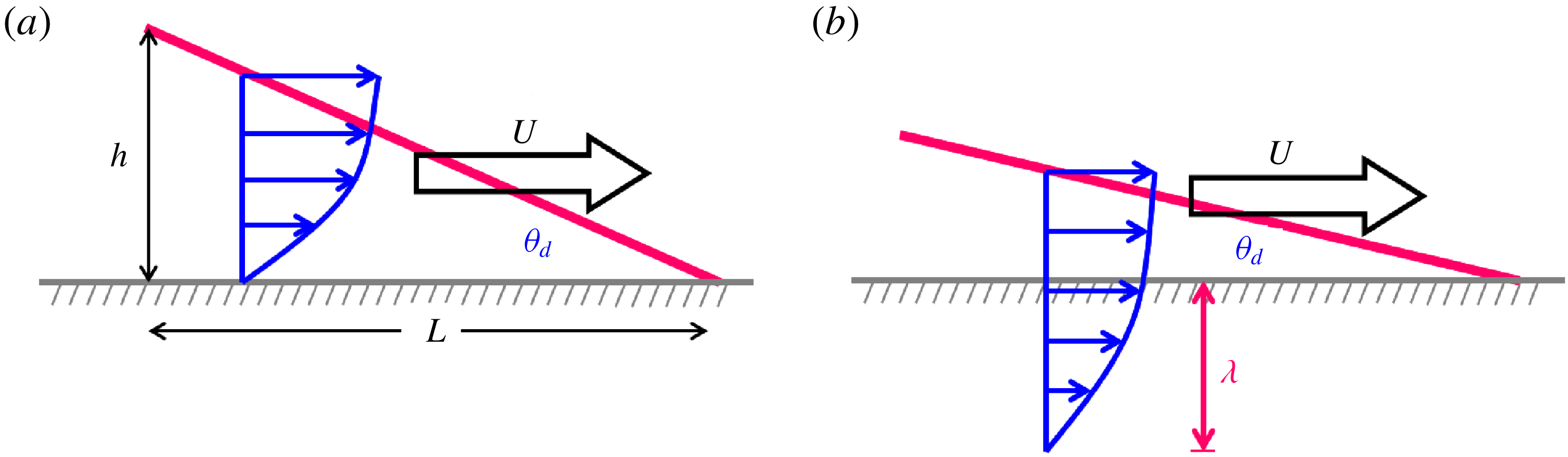
Consider a fluid wedge driven by a moving contact line at speed
 $U$
relative to the wall (see figure 1). The fluid viscosity is
 $\unicode[STIX]{x1D702}$
. The wedge opening angle is
 $\unicode[STIX]{x1D703}_{d}$
, representing the apparent dynamic contact angle. Here we focus on the complete wetting situation. So
 $\unicode[STIX]{x1D703}_{d}$
is assumed small throughout this work.
Local flow behaviours near advancing contact lines. (a) The no-slip case. (b) The strong-slip case.

We first review the no-slip case (figure 1
a). The contact line is driven by the surface tension force (per unit width)
 $\unicode[STIX]{x1D6FE}\unicode[STIX]{x1D703}_{d}^{2}$
with
 $\unicode[STIX]{x1D6FE}$
being the air–liquid interfacial tension. Tanner’s wetting law can be obtained by balancing this force to the viscous force (per unit width)
 $\unicode[STIX]{x1D702}U/h\times L$
over length
 $L$
with the corresponding height
 $h=L\unicode[STIX]{x1D703}_{d}$
:
 $$\begin{eqnarray}\unicode[STIX]{x1D703}_{d}\sim Ca^{1/3},\end{eqnarray}$$
where
 $Ca=\unicode[STIX]{x1D702}U/\unicode[STIX]{x1D6FE}$
is the capillary number and typically small. Relating the drop radius
 $R$
with
 $U\sim R/t$
and further applying the constant drop volume constraint
 $R^{3}\unicode[STIX]{x1D703}_{d}=\unicode[STIX]{x1D6FA}$
, this yields the well-known
 $1/10$
spreading law due to Tanner (Reference Tanner1979):
 $$\begin{eqnarray}R\sim \left(\frac{\unicode[STIX]{x1D6FA}^{3}\unicode[STIX]{x1D6FE}t}{\unicode[STIX]{x1D702}}\right)^{1/10}.\end{eqnarray}$$
When wall slip is present with slip length
 $\unicode[STIX]{x1D706}$
(figure 1
b), (2.1) is still a good approximation if
 $\unicode[STIX]{x1D706}$
is much smaller than the liquid height
 $h=L\unicode[STIX]{x1D703}_{d}$
. As the contact line advances,
 $\unicode[STIX]{x1D703}_{d}$
is gradually decreased and so is
 $Ca$
. When
 $\unicode[STIX]{x1D703}_{d}$
is decreased to the point where
 $h$
is comparable to
 $\unicode[STIX]{x1D706}$
, slip effects will start to become important. The contact angle at this point is
 $\unicode[STIX]{x1D703}_{d}\sim \unicode[STIX]{x1D706}/L$
, giving the critical capillary number below which Tanner’s wetting law (2.1) ceases to hold:
 $$\begin{eqnarray}Ca^{\ast }\sim (\unicode[STIX]{x1D706}/L)^{3}.\end{eqnarray}$$
Expression (2.3) also marks the no-slip-to-slip transition point. During this transition, the viscous stress scales as
 $\unicode[STIX]{x1D702}U/(h+\unicode[STIX]{x1D706})$
across
 $h+\unicode[STIX]{x1D706}$
, the distance of the interface to the extrapolated no-slip plane outside the wall. But as the contact line continues slowing down at
 $Ca$
below this point, we enter the strong-slip regime
 $h\ll \unicode[STIX]{x1D706}$
and the viscous stress is reduced to
 $\unicode[STIX]{x1D702}U/\unicode[STIX]{x1D706}$
. Balancing the corresponding viscous force
 $\unicode[STIX]{x1D702}U/\unicode[STIX]{x1D706}\times L$
to the surface tension force
 $\unicode[STIX]{x1D6FE}\unicode[STIX]{x1D703}_{d}^{2}$
, the wetting law is changed to
 $$\begin{eqnarray}\unicode[STIX]{x1D703}_{d}\sim Ca^{1/2}(L/\unicode[STIX]{x1D706})^{1/2}.\end{eqnarray}$$
Compared to (2.1) for the no-slip case, not only does
 $\unicode[STIX]{x1D703}_{d}$
vary as
 $Ca^{1/2}$
but also the additional length scale ratio
 $L/\unicode[STIX]{x1D706}$
is involved. The latter, from a dimensional point of view, must be the case because
 $\unicode[STIX]{x1D706}$
now enters to influence the macroscopic wetting characteristics.
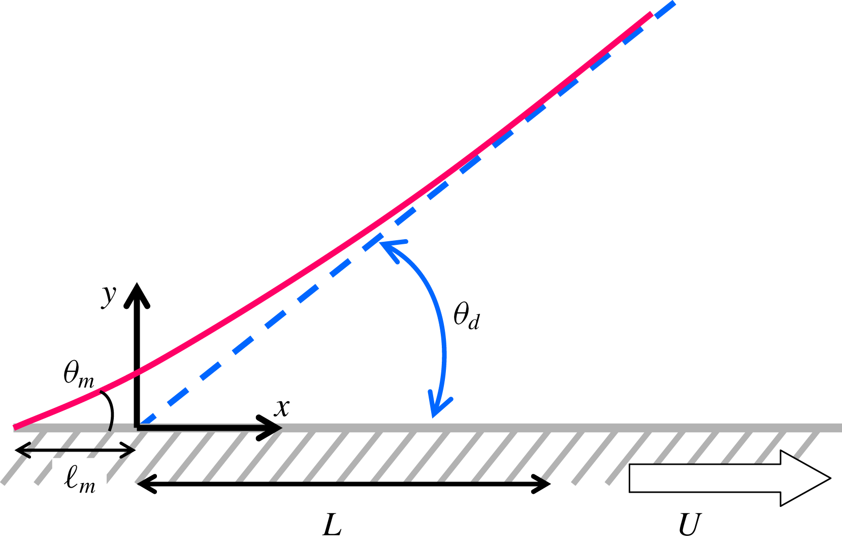
It is worth mentioning that a relationship similar to (2.4) can be equally applied to describe how the microscopic contact angle
 $\unicode[STIX]{x1D703}_{m}$
varies with the associated length
 $\ell _{m}$
(see figure 2) for the situation where
 $\unicode[STIX]{x1D706}$
is macroscopically small but microscopically large. In this case,
 $\unicode[STIX]{x1D703}_{d}$
and
 $L$
can be replaced respectively by
 $\unicode[STIX]{x1D703}_{m}$
and
 $\ell _{m}$
in (2.4):
 $$\begin{eqnarray}\unicode[STIX]{x1D703}_{m}\sim Ca^{1/2}(\ell _{m}/\unicode[STIX]{x1D706})^{1/2}.\end{eqnarray}$$
Its crossover to the macroscopic case (2.1),
 $\unicode[STIX]{x1D703}_{d}\sim Ca^{1/3}$
(by setting
 $\unicode[STIX]{x1D703}_{m}\sim \unicode[STIX]{x1D703}_{d}$
), provides an estimate for
 $\ell _{m}$
:
 $$\begin{eqnarray}\ell _{m}\sim \unicode[STIX]{x1D706}Ca^{-1/3}.\end{eqnarray}$$
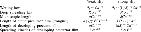
This is essentially the characteristic length found previously using the slip model (Eggers & Stone Reference Eggers and Stone2004). It is also the width of the ‘foot’ of a spreading polymer drop postulated by Brochard & de Gennes (Reference Brochard and de Gennes1984). On the contrary, for the no-slip case,
 $\ell _{m}$
is found to be
 ${\sim}aCa^{-2/3}$
due to precursor film (Hervet & de Gennes Reference Hervet and de Gennes1984; Eggers & Stone Reference Eggers and Stone2004), where
 $a$
is the molecular length. As will be shown in § 6.5, for a spreading polymer drop in which both slip and disjoining pressure coexist, the microscopic length is actually the ‘foot’ scale (2.6) rather than that of the precursor film.
A wedge-like free-surface flow near an advancing contact line. The figure is drawn in the frame moving with the contact line at speed
 $U$
.

The spreading law corresponding to (2.4) can be readily found by taking
 $L\sim R$
and
 $U\sim R/t$
under the constant-volume constraint
 $R^{3}\unicode[STIX]{x1D703}_{0}=\unicode[STIX]{x1D6FA}$
:
 $$\begin{eqnarray}R\sim \left(\frac{\unicode[STIX]{x1D6FA}^{2}\unicode[STIX]{x1D706}\unicode[STIX]{x1D6FE}t}{\unicode[STIX]{x1D702}}\right)^{1/8}.\end{eqnarray}$$
The same
 $1/8$
power law has been briefly mentioned by Brochard & de Gennes (Reference Brochard and de Gennes1984). The main result of their work is that wall slip can lead to the existence of a ‘foot’ of thickness
 $\unicode[STIX]{x1D706}$
bridging between the central spherical cap and the precursor film. When
 $h<\unicode[STIX]{x1D706}$
, the foot will merge with the cap. In this case they merely gave the
 $1/8$
power law for the spreading kinetics without mentioning how the dynamic contact angle changes its behaviour. The present work is to fill this gap.
3 Hydrodynamics of a slipping contact line
To derive the actual relationship of the apparent dynamic contact angle
 $\unicode[STIX]{x1D703}_{d}$
with the wetting speed
 $U$
, we consider the local fluid motion around an advancing contact line in the frame moving with
 $-U$
, as shown in figure 2. The fluid motion takes place within a horizontal scale
 $L$
at which the interface can be kept roughly as a straight wedge under
 $Ca\ll 1$
(Snoeijer Reference Snoeijer2006). So
 $\unicode[STIX]{x1D703}_{d}$
can be deemed as the slope of the interface that varies slowly with respect to the wedge (Snoeijer Reference Snoeijer2006). In the case of a spreading drop,
 $L$
can be roughly taken as
 $cR$
in proportion to the drop radius
 $R$
with
 $c<1$
. So
 $L$
is essentially chosen as the length scale that bridges the macroscopic region far away from the contact line. In practice,
 $L$
can be taken at the inflection point of the interface that changes from concave to convex shape (Kavehpour, Ovryn & McKinley Reference Kavehpour, Ovryn and McKinley2003; Pahlavan et al.
Reference Pahlavan, Cueto-Felgueroso, McKinley and Juanes2015). Another reason why we want to choose
 $L$
in this way is that, as suggested from (2.4), this will allow us to capture the size-dependent
 $\unicode[STIX]{x1D703}_{d}$
for a strongly slipping drop, which will be shown in § 4.2.
Since
 $\unicode[STIX]{x1D703}_{d}$
is small and hence the liquid height
 $h(x)$
, this allows us to use the lubrication theory to formulate the problem. The horizontal velocity
 $u$
satisfies the momentum equation
 $$\begin{eqnarray}p_{x}=\unicode[STIX]{x1D702}u_{yy}.\end{eqnarray}$$
Here the pressure
 $p$
is given by the Laplace pressure
 $$\begin{eqnarray}p=-\unicode[STIX]{x1D6FE}h_{xx},\end{eqnarray}$$
where
 $\unicode[STIX]{x1D6FE}$
is the surface tension. The system is subject to the following boundary conditions. On the solid surface, the Navier slip condition is assumed (Navier Reference Navier1823):
 $$\begin{eqnarray}\text{at }y=0,\quad u-U=\unicode[STIX]{x1D706}u_{y},\end{eqnarray}$$
where
 $\unicode[STIX]{x1D706}$
is the slip length. At the air–liquid interface, it is basically stress-free:
 $$\begin{eqnarray}\text{at }y=h(x),\quad u_{y}=0.\end{eqnarray}$$
The solution satisfying (3.1), (3.3) and (3.4) is
 $$\begin{eqnarray}u=\frac{p_{x}}{2\unicode[STIX]{x1D702}}(y^{2}-2hy-2\unicode[STIX]{x1D706}h)+U.\end{eqnarray}$$
The above flow field must fulfil the requirement that there is no net flow rate across the wedge, i.e.
 $\int _{0}^{h}u\,\text{d}y=0$
. This together with (3.2) leads to the following equation governing the interface profile in the vicinity of the contact line:
 $$\begin{eqnarray}h^{\prime \prime \prime }=-\frac{3Ca}{h^{2}+3\unicode[STIX]{x1D706}h},\end{eqnarray}$$
where primes mean spatial derivatives.
We should point out that the slip length
 $\unicode[STIX]{x1D706}$
here cannot be arbitrarily large. The reason is that in deriving (3.6), we have employed the standard lubrication approximation (3.1) in which the lateral viscous term
 $\unicode[STIX]{x1D702}u_{xx}$
is neglected. However, if
 $\unicode[STIX]{x1D706}$
gets too large, one would end up with a plug flow across the wedge, which might lose lubrication. Specifically, drag reduction introduced by
 $\unicode[STIX]{x1D706}$
makes the fluid move as if it had a reduced effective viscosity
 $\unicode[STIX]{x1D702}_{eff}\sim \unicode[STIX]{x1D702}/(1+3\unicode[STIX]{x1D706}/h)$
across the liquid height
 $h$
(Liao et al.
Reference Liao, Li and Wei2013; Li et al.
Reference Li, Liao, Wen and Wei2014). The corresponding transverse viscous contribution
 $\unicode[STIX]{x1D702}_{eff}u_{yy}$
thus scales as
 $\unicode[STIX]{x1D702}_{eff}U/h^{2}\sim \unicode[STIX]{x1D702}U/h^{2}\times (1+3\unicode[STIX]{x1D706}/h)^{-1}$
. For large
 $\unicode[STIX]{x1D706}$
,
 $\unicode[STIX]{x1D702}_{eff}u_{yy}$
is reduced to
 ${\sim}\unicode[STIX]{x1D702}U/(\unicode[STIX]{x1D706}h)$
which could be outweighed by the lateral contribution without slip
 $\unicode[STIX]{x1D702}u_{xx}\sim \unicode[STIX]{x1D702}U/L^{2}$
. In this case, the driving surface tension force will not be balanced by the viscous force through the velocity gradient across
 $\unicode[STIX]{x1D706}$
. Hence, to prevent the above from happening, it is necessary to assume
 $\unicode[STIX]{x1D702}_{eff}u_{yy}\gg \unicode[STIX]{x1D702}u_{xx}$
. This yields
 $$\begin{eqnarray}\unicode[STIX]{x1D706}h/L^{2}\ll 1\quad \text{or}\quad \unicode[STIX]{x1D706}/L\ll 1/\unicode[STIX]{x1D703}_{d},\end{eqnarray}$$
which restricts the size of
 $\unicode[STIX]{x1D706}$
below which the present lubrication analysis holds. In most situations,
 $\unicode[STIX]{x1D706}/L\ll 1$
, so (3.7) is always satisfied. For much larger slip lengths beyond (3.7), possible inertial effects may arise from much faster slipping flows (Münch et al.
Reference Münch, Wagner and Witelski2005).
For
 $\unicode[STIX]{x1D706}=0$
, equation (3.6) is reduced to the well-known Tanner equation (Tanner Reference Tanner1979). For this no-slip case, it has been shown by Duffy & Wilson (Reference Duffy and Wilson1997) that an analytical solution can exist in terms of Airy functions, showing the possibility of a non-zero curvature in the far field. Equation (3.6) can also describe the motion of a receding contact line (Eggers Reference Eggers2005b
) with
 $Ca$
replaced by
 $-Ca$
. In this case, there exists a critical
 $Ca$
above which the contact line vanishes to give rise to the formation of a continuous thin film over the surface (Eggers Reference Eggers2005b
).
Eggers (Reference Eggers2004) solved (3.6) for partial wetting fluids under
 $Ca\ll \unicode[STIX]{x1D703}_{e}^{3}$
with
 $\unicode[STIX]{x1D703}_{e}$
being the equilibrium contact angle. He obtained the following dynamic contact angle relationship:
 $$\begin{eqnarray}h^{\prime 3}(x)=\unicode[STIX]{x1D703}_{e}^{3}+9Ca\ln \left(\frac{xe\unicode[STIX]{x1D703}_{e}}{3\unicode[STIX]{x1D706}}\right).\end{eqnarray}$$
A similar expression was also obtained by Hocking (Reference Hocking1992). Equation (3.8) is essentially the Tanner–Cox–Voinov law (see (4.10b
)) (Voinov Reference Voinov1976; Tanner Reference Tanner1979; Cox Reference Cox1986) and the slip length
 $\unicode[STIX]{x1D706}$
merely contributes in the logarithmic factor. However, because (3.8) is derived under
 $Ca\ll \unicode[STIX]{x1D703}_{e}^{3}$
, it can only describe the dynamic contact angle
 $h^{\prime }(x)=\unicode[STIX]{x1D703}_{d}$
slightly greater than
 $\unicode[STIX]{x1D703}_{e}$
. So the dynamic contact angle in his work is located in the regime
 $\unicode[STIX]{x1D703}_{d}^{3}\gg Ca$
.
In contrast to Eggers (Reference Eggers2004), we will look at the complete wetting scenario where
 $\unicode[STIX]{x1D703}_{d}^{3}\sim Ca$
or smaller. In this case, Hocking (Reference Hocking1992) considered the case of a weakly slipping drop and obtained a wetting law slightly different from (3.8). In this work we will extend to the case of a strongly slipping drop whose height is smaller than the slip length
 $\unicode[STIX]{x1D706}$
. Below we use (3.6) to derive a generalized dynamic contact angle relationship for an arbitrary value of
 $\unicode[STIX]{x1D706}$
under (3.7). As will be shown next, we will not only recover the well-known Tanner–Cox–Voinov law corresponding to (2.1), but also obtain a precise form of the strong-slip wetting law corresponding to (2.4).
4 Generalized dynamic contact angle relationship: bridging Tanner’s law and the strong-slip law
We first non-dimensionalize (3.6) with
 $$\begin{eqnarray}H=h/3\unicode[STIX]{x1D706}\quad \text{and}\quad z=x/L.\end{eqnarray}$$
Recall that
 $L$
here is chosen as the length scale at which the interface can be kept roughly as a straight wedge under
 $Ca\ll 1$
. We are interested in the contact line characteristics on this length scale because
 $\unicode[STIX]{x1D706}$
can be comparable to or larger than the wedge height
 $h(x=L)=L\unicode[STIX]{x1D703}_{d}$
. Also for this reason, we scale
 $h$
by
 $3\unicode[STIX]{x1D706}$
so that
 $1/H=3\unicode[STIX]{x1D706}/h$
can reflect the extent of wall slip.
With (4.1), (3.6) is transformed to
 $$\begin{eqnarray}H^{\prime \prime \prime }(z)=-\frac{3\unicode[STIX]{x1D6FF}}{H^{2}+H},\end{eqnarray}$$
where
 $\unicode[STIX]{x1D6FF}$
is the rescaled capillary number and defined as
 $$\begin{eqnarray}\unicode[STIX]{x1D6FF}=Ca(L/3\unicode[STIX]{x1D706})^{3}.\end{eqnarray}$$
Here
 $\unicode[STIX]{x1D6FF}^{1/3}=Ca^{1/3}L/3\unicode[STIX]{x1D706}$
can be understood as the ratio of the no-slip liquid thickness
 $h\sim L\unicode[STIX]{x1D703}_{d}\sim LCa^{1/3}$
to the slip length
 $\unicode[STIX]{x1D706}$
. Alternatively, it can also be interpreted as the ratio of
 $L$
to the ‘foot’ scale
 $\unicode[STIX]{x1D706}Ca^{-1/3}$
. So
 $1/\unicode[STIX]{x1D6FF}$
can be used to measure the extent of wall slip at the macroscopic level. Ratio
 $\unicode[STIX]{x1D6FF}\gg 1$
means weak slip with
 $h\gg \unicode[STIX]{x1D706}\,(H\gg 1)$
, whereas
 $\unicode[STIX]{x1D6FF}\ll 1$
represents strong slip with
 $h\ll \unicode[STIX]{x1D706}\,(H\ll 1)$
. When
 $\unicode[STIX]{x1D6FF}\sim O(1)$
, it is the no-slip-to-slip transition point (2.3) at which
 $h\sim \unicode[STIX]{x1D706}(H\sim O(1))$
.
To solve (4.2), we will use the ‘slowly varying slope’ approach due originally to Voinov (Reference Voinov1976). This approach has been rigorously justified by Snoeijer (Reference Snoeijer2006) who developed a long-wavelength theory beyond the lubrication theory to solve for free-surface wedge-like flows with large slopes. He pointed out that the validity of this approach lies in
 $Ca\ll 1$
under which surface tension dominates over viscosity. This condition ensures that the interface is merely slightly deformed from a straight wedge due to viscosity, making its curvature
 $\unicode[STIX]{x1D705}\approx \unicode[STIX]{x2202}_{x}\unicode[STIX]{x1D703}$
vary slowly with respect to the relevant length scales, where
 $\unicode[STIX]{x1D703}(x)\equiv h^{\prime }(x)$
is the local slope and not necessarily small. Specifically, small variations of
 $\unicode[STIX]{x1D705}$
can produce an error to the solution at an order of
 $L\unicode[STIX]{x1D705}\sim L\unicode[STIX]{x2202}_{x}\unicode[STIX]{x1D703}=(L/h)\times h\unicode[STIX]{x2202}_{x}\unicode[STIX]{x1D703}$
. Thus, the measure of
 $\unicode[STIX]{x1D705}$
with respect to
 $h$
,
 $h\unicode[STIX]{x2202}_{x}\unicode[STIX]{x1D703}$
, has to be sufficiently small to ensure a valid asymptotic expansion (in small
 $\unicode[STIX]{x1D700}\equiv L\unicode[STIX]{x2202}_{x}\unicode[STIX]{x1D703}$
), as also shown in Snoeijer’s analysis. Further establishing that the problem at leading order can be reduced to that of a straight wedge, he was able to show that in the small
 $Ca$
limit the dynamic contact angle relationship exactly recovers the well-known result reported by Voinov (Reference Voinov1976) and Cox (Reference Cox1986). If
 $\unicode[STIX]{x1D703}$
is already small as in the complete wetting scenario considered here, the error
 $L\unicode[STIX]{x2202}_{x}\unicode[STIX]{x1D703}$
will be even smaller, making this longwave approach even more suitable to such small-slope situation. The robustness of this approach has also been recently demonstrated in analysing the unusual wetting dynamics due to surfactant superspreaders (Wei Reference Wei2018).
Now consider the application of Snoeijer’s longwave approach to our problem in which complete wetting is assumed. In the case of no slip, the error due to curvature variations is
 $L\unicode[STIX]{x2202}_{x}\unicode[STIX]{x1D703}\sim \unicode[STIX]{x1D703}_{d}\sim Ca^{1/3}$
according to (2.1). When wall slip is present, because it tends to promote wetting, the liquid would become even flatter, making the error even smaller. For the strong-slip case where
 $h\ll \unicode[STIX]{x1D706}$
, the measure of the interface curvature
 $\unicode[STIX]{x1D705}\sim \unicode[STIX]{x2202}_{x}\unicode[STIX]{x1D703}$
has to be small with respect to
 $\unicode[STIX]{x1D706}$
, giving
 $\unicode[STIX]{x1D706}\unicode[STIX]{x2202}_{x}\unicode[STIX]{x1D703}\ll 1$
under which a valid asymptotic expansion can be made. It also restricts the size of
 $\unicode[STIX]{x1D706}$
to ensure that the surface tension force can be balanced by the viscous force through the velocity gradient across
 $\unicode[STIX]{x1D706}$
. Indeed, in terms of scaling,
 $\unicode[STIX]{x1D706}\unicode[STIX]{x2202}_{x}\unicode[STIX]{x1D703}\sim \unicode[STIX]{x1D706}\unicode[STIX]{x1D703}_{d}/L\ll 1$
, which is exactly (3.7). The corresponding error is
 $L\unicode[STIX]{x2202}_{x}\unicode[STIX]{x1D703}\sim \unicode[STIX]{x1D703}_{d}\sim Ca^{1/2}(L/\unicode[STIX]{x1D706})^{1/2}$
according to (2.4). Also because such a strong-slip scenario occurs at
 $Ca<Ca^{\ast }\sim (\unicode[STIX]{x1D706}/L)^{3}$
from (2.3), the error will be no larger than
 $O(Ca^{1/3})$
. Together with the fact that the error for the no-slip case is also
 $O(Ca^{1/3})$
, we conclude that the largest error with and without slip is
 $\unicode[STIX]{x1D700}=O(Ca^{1/3})$
, consistent with the formal small slope theory given by Snoeijer (Reference Snoeijer2006). In appendix A we extend Snoeijer’s theory to provide a formal asymptotic theory for the case with slip, showing that self-consistent asymptotic expansions for weak slip and strong slip can be constructed respectively with
 $\unicode[STIX]{x1D700}=Ca^{1/3}$
and
 $\unicode[STIX]{x1D700}=Ca^{1/3}\,(h^{\ast }/\unicode[STIX]{x1D706})^{1/3}$
(with
 $h^{\ast }$
being the characteristic transverse length scale). The error
 $Ca^{1/3}\,(h^{\ast }/\unicode[STIX]{x1D706})^{1/3}$
for the strong-slip case with
 $h^{\ast }/\unicode[STIX]{x1D706}\ll 1$
is indeed smaller than
 $Ca^{1/3}$
for the weak-slip case.
In what follows, we use a slightly different approach but in the same spirit as Snoeijer’s to derive a generalized dynamic contact angle relationship to bridge both weak-slip and strong-slip cases. Specifically, instead of solving the equation in term of
 $z$
, we solve it in terms of
 $H$
by changing variable. As can be seen below, this approach will not only provide a more straightforward way to recover the Tanner–Cox–Voinov law (4.10b
), but also allow us to derive the new strong-slip wetting law (4.11b
).
We first integrate both sides of (4.2). This yields
 $$\begin{eqnarray}H^{\prime \prime }=-3\unicode[STIX]{x1D6FF}\int _{z_{\infty }}^{z}\frac{\text{d}z}{H^{2}+H},\end{eqnarray}$$
wherein we have used
 $H^{\prime \prime }(z_{\infty })=0$
with
 $z_{\infty }=x_{\infty }/L\gg 1$
. On the right-hand side of (4.4), we can use
 $\text{d}z=\text{d}H/H^{\prime }$
to transform the integral with respect to
 $H$
. As discussed earlier, since
 $Ca\ll 1$
here, the wedge is merely slightly deformed with small variations of its curvature:
 $$\begin{eqnarray}Lh_{xx}=(3\unicode[STIX]{x1D706}/L)H^{\prime \prime }=Ca^{1/3}\unicode[STIX]{x1D6FF}^{-1/3}H^{\prime }\text{d}H^{\prime }/\text{d}H\ll 1.\end{eqnarray}$$
In the last expression, we have rewritten
 $(3\unicode[STIX]{x1D706}/L)$
and
 $H^{\prime \prime }$
in terms of
 $\unicode[STIX]{x1D6FF}$
and
 $H^{\prime }$
using (4.3) and
 $H^{\prime \prime }=H^{\prime }\text{d}H^{\prime }/\text{d}H$
. As will be justified a posteriori, either
 $\text{d}H^{\prime }/\text{d}z\ll 1$
(when
 $H^{\prime }$
is small for
 $\unicode[STIX]{x1D6FF}\ll 1$
) or
 $\text{d}H^{\prime }/\text{d}H\ll 1$
(when
 $H^{\prime }$
is large for
 $\unicode[STIX]{x1D6FF}\gg 1$
) guarantees (4.5). This allows us to treat
 $H^{\prime }$
as a slowly varying function, which will also be confirmed a posteriori. So the integral in (4.4) can be approximated as
 $$\begin{eqnarray}\int _{z_{\infty }}^{z}\frac{\text{d}z}{H^{2}+H}\approx \frac{1}{H^{\prime }}\int _{H_{\infty }}^{H}\frac{\text{d}H}{H^{2}+H},\end{eqnarray}$$
where
 $H_{\infty }\equiv H(z_{\infty })=h_{\infty }/3\unicode[STIX]{x1D706}=x_{\infty }\unicode[STIX]{x1D703}_{d}/3\unicode[STIX]{x1D706}$
(with
 $x_{\infty }\gg L$
).
Evaluating the above integral, substituting it into (4.4) and replacing
 $H^{\prime \prime }=H^{\prime }\text{d}H^{\prime }/\text{d}H$
, (4.4) becomes
 $$\begin{eqnarray}H^{\prime 2}\frac{\text{d}H^{\prime }}{\text{d}H}=-3\unicode[STIX]{x1D6FF}\ln \left(\frac{1+H_{\infty }^{-1}}{1+H^{-1}}\right).\end{eqnarray}$$
Integrating both sides of (4.7) with respect to
 $H$
, we can obtain the following dynamic contact angle relationship valid for an arbitrary value of
 $\unicode[STIX]{x1D706}$
(under the constraint (3.7)):
 $$\begin{eqnarray}H^{\prime 3}(z)=H_{1}^{\prime 3}+9\unicode[STIX]{x1D6FF}[F(H_{1},H_{\infty })-F(H,H_{\infty })],\end{eqnarray}$$
or its dimensional form
 $$\begin{eqnarray}h^{\prime 3}(x)=h_{1}^{\prime 3}+9Ca[F(h_{1}/3\unicode[STIX]{x1D706},h_{\infty }/3\unicode[STIX]{x1D706})-F(h/3\unicode[STIX]{x1D706},h_{\infty }/3\unicode[STIX]{x1D706})].\end{eqnarray}$$
Here the function
 $F(H,H_{\infty })$
is given by
 $$\begin{eqnarray}F(H,H_{\infty })=H\ln [H(1+1/H_{\infty })]-(H+1)\ln (H+1).\end{eqnarray}$$
In (4.8b
), the apparent dynamic contact angle
 $\unicode[STIX]{x1D703}_{d}=h^{\prime }(x)$
is evaluated at
 $x$
much larger than the microscopic scale
 $x_{1}$
that is taken
 $O(\unicode[STIX]{x1D706}/L)$
or smaller. But macroscopically,
 $x$
also has to be much smaller than
 $x_{\infty }$
that is chosen to be much greater than the bridging length
 $L$
.
Next we inspect two limiting cases: (i) weak slip:
 $\unicode[STIX]{x1D6FF}\gg 1$
that will recover the well-known Tanner–Cox–Voinov law and (ii) strong slip:
 $\unicode[STIX]{x1D6FF}\ll 1$
for which a new wetting law will be derived. This will also clearly reveal how one limit changes to the other.
4.1 Weak slip
First of all, we notice that
 $F(H)$
given by (4.9) will scale as
 $\ln (H)$
for large
 $H$
but turn into
 $H\ln (H)$
when
 $H$
is small. So for
 $\unicode[STIX]{x1D6FF}\gg 1$
,
 $H^{\prime 3}\sim \unicode[STIX]{x1D6FF}\cdot F$
from (4.8a
) demands that
 $H=h/3\unicode[STIX]{x1D706}$
has to be large, meaning that the contact line motion will be mainly described by Tanner’s weak-slip characteristics. In fact, why
 $\unicode[STIX]{x1D6FF}\gg 1$
must lead to
 $H\gg 1$
and vice versa can be immediately seen from the alternative form of (4.2):
 $H^{2}H^{\prime \prime \prime }=-3\unicode[STIX]{x1D6FF}/(1+H^{-1})$
. When
 $H\gg 1$
, the above form is reduced to
 $H^{2}H^{\prime \prime \prime }=-3\unicode[STIX]{x1D6FF}$
whose scaling form
 $(H/z)^{3}\sim \unicode[STIX]{x1D6FF}$
is essentially (2.1). To show this exactly, because
 $F(H,H_{\infty })-F(H_{1},H_{\infty })\approx -\ln (H/H_{1})$
for
 $H\gg 1$
, (4.8a
) is reduced to
 $$\begin{eqnarray}H^{\prime 3}(z)=H_{1}^{\prime 3}+9\unicode[STIX]{x1D6FF}\ln (H/H_{1}).\end{eqnarray}$$
Equation (4.10a
) indicates that
 $\text{d}H^{\prime }/\text{d}H=(1/3)(9\unicode[STIX]{x1D6FF})^{1/3}H^{-1}[\ln (H/H_{1})]^{-2/3}$
. Since
 $H\sim [\unicode[STIX]{x1D6FF}\ln (\unicode[STIX]{x1D6FF}^{1/3})]^{1/3}$
according to (4.10a
) (with
 $z\sim O(1)$
and
 $H_{1}\sim O(1)$
because of
 $h_{1}\sim \unicode[STIX]{x1D706}$
),
 $\text{d}H^{\prime }/\text{d}H\sim [\ln (\unicode[STIX]{x1D6FF}^{1/3})]^{-1}\ll 1$
with
 $\unicode[STIX]{x1D6FF}\gg 1$
here. So
 $H^{\prime }$
indeed varies slowly with respect to
 $H$
, justifying (4.6) for deriving (4.10a
). In terms of the curvature, (4.5) indicates that
 $Lh_{xx}=Ca^{1/3}\unicode[STIX]{x1D6FF}^{-1/3}H^{\prime }\text{d}H^{\prime }/\text{d}H\sim Ca^{1/3}[\ln (\unicode[STIX]{x1D6FF}^{1/3})]^{-2/3}\ll 1$
. The actual slope
 $h_{x}=(3\unicode[STIX]{x1D706}/L)H^{\prime }\sim Ca^{1/3}[\ln (\unicode[STIX]{x1D6FF}^{1/3})]^{1/3}$
can be deemed nearly constant (with error of
 $O(Lh_{xx})$
). Also for this reason,
 $\ln (H/H_{1})$
in (4.10a
) can be reasonably approximated as
 $\ln (x/x_{1})$
, as also employed by previous studies (Voinov Reference Voinov1976; de Gennes Reference de Gennes1986; Eggers Reference Eggers2004).
Writing (4.10a
) back to the dimensional form together with the approximation
 $\ln (h/h_{1})\approx \ln (x/x_{1})$
(with
 $x_{1}\ll x\ll x_{\infty }$
), we recover the well-known Tanner–Cox–Voinov law (Voinov Reference Voinov1976; Tanner Reference Tanner1979; Cox Reference Cox1986):
 $$\begin{eqnarray}h^{\prime 3}(x)=h_{1}^{\prime 3}+9Ca\ln (x/x_{1}).\end{eqnarray}$$
Note that
 $\unicode[STIX]{x1D706}$
here is not zero but small compared to
 $h$
. So it will provide a natural microscopic length
 $x_{1}$
to prevent the stress singularity at the contact line. This length can be taken as
 $x_{1}\approx h_{1}/\unicode[STIX]{x1D703}_{d}$
with
 $h_{1}\approx \unicode[STIX]{x1D706}$
, giving
 $x_{1}\sim \unicode[STIX]{x1D706}/\unicode[STIX]{x1D703}_{d}$
(de Gennes Reference de Gennes1985). Taking
 $\unicode[STIX]{x1D703}_{d}\sim Ca^{1/3}$
, the length becomes
 $x_{1}\sim \unicode[STIX]{x1D706}Ca^{-1/3}$
given by (2.6) (Eggers & Stone Reference Eggers and Stone2004). In fact,
 $\unicode[STIX]{x1D706}Ca^{-1/3}$
is the size of the ‘foot’ (Brochard & de Gennes Reference Brochard and de Gennes1984) and represents the characteristic wetting length arising from slip. As can be seen throughout this work, the ‘foot’ will play vital roles in the characteristics of a slipping contact line.
4.2 Strong slip
For
 $\unicode[STIX]{x1D6FF}\ll 1$
, since
 $H^{\prime 3}\sim \unicode[STIX]{x1D6FF}\cdot F$
from (4.8a
) requires
 $H=h/3\unicode[STIX]{x1D706}$
to be small, slip effects will strongly influence the contact line dynamics. The rewritten form of (4.2),
 $H^{2}H^{\prime \prime \prime }=-3\unicode[STIX]{x1D6FF}/(1+H^{-1})$
, now reduces to
 $HH^{\prime \prime \prime }=-3\unicode[STIX]{x1D6FF}$
when
 $H\ll 1$
. The scaling form of the latter,
 $H^{2}/z^{3}\sim \unicode[STIX]{x1D6FF}$
, re-conforms the strong-slip scaling (2.4). The precise solution form for
 $H^{\prime }$
can be obtained using (4.8a
) with
 $H\ll H_{\infty }\ll 1$
. In this case, because
 $F(H,H_{\infty })\approx H\ln (H/H_{\infty })$
from (4.9), it dominates (4.8a
) and
 $F(H_{1},H_{\infty })\approx H_{1}\ln (H_{1}/H_{\infty })$
is negligible. So (4.8a
) is reduced to
 $$\begin{eqnarray}H^{\prime 2}(z)=H_{1}^{\prime 3}/H^{\prime }+9\unicode[STIX]{x1D6FF}(H/H^{\prime })\ln (H_{\infty }/H).\end{eqnarray}$$
Equation (4.11a
) reveals that
 $H\sim \unicode[STIX]{x1D6FF}^{1/2}[\ln (\unicode[STIX]{x1D6FF}^{-1/2})]^{1/2}\ll 1$
(with
 $z\sim O(1)$
and
 $H_{\infty }\sim O(1)$
because of
 $h_{\infty }\,\unicode[STIX]{x1D706}$
). Since
 $H^{\prime \prime }=\text{d}H^{\prime }/\text{d}z\sim O(H)$
is also small,
 $H^{\prime }$
varies slowly with respect to
 $z$
. This not only justifies (4.6) for deriving (4.11a
), but also allows us to use the approximation
 $H\approx H^{\prime }z$
on the right-hand side of (4.11a
). As the actual slope
 $h_{x}=(3\unicode[STIX]{x1D706}/L)H^{\prime }$
becomes even smaller, this guarantees (4.5). Because most situations are not far from either
 $\unicode[STIX]{x1D6FF}\gg 1$
or
 $\unicode[STIX]{x1D6FF}\ll 1$
and also given that these two limits are shown to satisfy the small-curvature condition (4.5), the general result (4.8b
) obtained by this ‘slowly varying slope’ approach should fairly capture the behaviour of the dynamic contact angle for an arbitrary value of
 $\unicode[STIX]{x1D706}$
under (3.7).
Writing (4.11a
) in the dimensional form with
 $(h_{\infty },h)\approx h^{\prime }(x_{\infty },x)$
(with
 $x\ll x_{\infty }$
), we arrive at
 $$\begin{eqnarray}h^{\prime 2}(x)=h_{1}^{\prime 3}/h^{\prime }+3Ca(x/\unicode[STIX]{x1D706})\ln (x_{\infty }/x),\end{eqnarray}$$
which gives the complete form for (2.4). Note here that the logarithmic term vanishes as
 $x\rightarrow 0$
– there is no microscopic length
 $x_{1}$
needed for regularizing that term because the viscous stress has already been regularized by slip. But in terms of the microstructure of the contact line, the inner region of width
 $x_{1}\ll L$
may enter to be part of the description. This is true when a precursor film exists due to disjoining pressure (see § 6).
As revealed by (4.11b
), the slope
 $h^{\prime }\approx (3Ca\,x/\unicode[STIX]{x1D706})^{1/2}[\ln (x_{\infty }/x)]^{1/2}$
near the contact line, owing to its involving the additional slip length
 $\unicode[STIX]{x1D706}$
, is not constant but varies as
 $x^{1/2}$
. The resulting interface profile is
 $h\approx (2/\surd 3)\unicode[STIX]{x1D706}Ca^{1/2}(x/\unicode[STIX]{x1D706})^{3/2}[\ln (x_{\infty }/x)]^{1/2}$
. Note that although this profile deviates from the linear wedge, since
 $h^{\prime }$
is small here, the amount of the deviation is small in the scale of
 $L$
, which is a consequence of the present ‘slowly varying slope’ approach. Now because
 $h\ll \unicode[STIX]{x1D706}$
, this requires
 $x\ll \unicode[STIX]{x1D706}Ca^{-1/3}$
in (4.11b
). So (4.11b
) has to be evaluated at a position much smaller than the ‘foot’ of size given by Brochard & de Gennes (Reference Brochard and de Gennes1984):
 $$\begin{eqnarray}\ell _{F}\sim \unicode[STIX]{x1D706}Ca^{-1/3}.\end{eqnarray}$$
In fact,
 $\unicode[STIX]{x1D6FF}\ll 1$
for this strong-slip case based on (4.3) means that the ‘foot’ has grown to a size much greater than
 $L$
, i.e.
 $\ell _{F}\gg L$
. So from the perspective of the ‘foot’, the interface profile described by (4.11b
) is essentially the ‘inner’ portion of the much larger ‘foot’. So the apparent contact angle (4.11b
) for a slipping drop can be thought of as the ‘microscopic’ contact angle of the ‘foot’. Thus it can be reasonably represented by
 $h^{\prime }(x=L\ll \ell _{F})$
and hence has the scaling form (2.4). The specific value of
 $L=c_{1}R$
can in principle be determined by solving the drop problem from which the constant
 $c_{1}$
can be found to measure the size of
 $L$
relative to the drop radius
 $R$
. As such, the apparent dynamic contact angle for this strong-slip situation is still well defined albeit its behaviour is coupled to that of the drop.
Moreover, given that the drop now becomes the ‘inner’ portion of the much larger ‘foot’, the interface profile described by (4.11b
) should also asymptotically approach the ‘foot’ as
 $x\rightarrow \infty$
, giving
 $x_{\infty }\sim \ell _{F}$
in the logarithmic term in (4.11b
). Combining the features anticipated above, for a strongly slipping thin drop with
 $h\ll \unicode[STIX]{x1D706}$
, its apparent dynamic contact angle evaluated from (4.11b
) (by neglecting
 $h_{1}^{\prime 3}$
) should take the form
 $$\begin{eqnarray}\unicode[STIX]{x1D703}_{d}^{2}=3Ca\left(\frac{c_{1}R}{\unicode[STIX]{x1D706}}\right)\ln \left(\frac{c_{2}\unicode[STIX]{x1D706}}{Ca^{1/3}R}\right).\end{eqnarray}$$
We emphasize that (4.13) is not limited to a strongly slipping thin drop. Since (4.13) is also the contact angle of the much larger ‘foot’, as we will show in § 6.5, it is equally applicable to the inner region of a weakly slipping thick drop within which the slip length can be microscopically large to affect the much thinner precursor film ahead of the ‘foot’. In this case,
 $\unicode[STIX]{x1D703}_{d}$
and
 $R$
in (4.13) should be replaced by the microscopic contact angle
 $\unicode[STIX]{x1D703}_{m}$
and the associated local length scale.
It is worth mentioning that Hocking (Reference Hocking1992) has solved essentially the same equation (4.2) for a weakly slipping drop and obtained the apparent dynamic contact angle relationship like (4.10b
) at
 $Ca\gg Ca^{\ast }$
. In contrast to his study, (4.13) derived for
 $Ca\ll Ca^{\ast }$
can describe not only the behaviour of a strongly slipping contact line, but also the ‘inner’ behaviour of a weakly slipping contact line, which complements Hocking’s result. In § 6.5, we solve the microscopic equation numerically, confirming that (4.13) is indeed the law for a contact line experiencing strong slip effects.
Note also that for a strongly slipping drop with
 $R\ll \ell _{F}$
or
 $R\sim \ell _{F}$
, because of the lack of separation between ‘foot’ and the central cap, the drop may display a bell shape with a concave rim (Brochard & de Gennes Reference Brochard and de Gennes1984). This causes an asphericity to the drop shape. Similar impacts of wall slip on the interface profile can also be seen in a dewetting drop on a slippery surface (Chan et al.
Reference Chan, McGraw, Salez, Seemann and Brinkmann2017).
4.3 Role of the ‘foot’ in dynamic contact angle with slip
To summarize the features in both §§ 4.1 and 4.2, it is actually the ‘foot’ length
 $\ell _{F}\sim \unicode[STIX]{x1D706}Ca^{-1/3}$
that separates weak slip and strong slip according to its ratio to the macroscopic length
 $L$
, i.e.
 $L/\ell _{F}\sim \unicode[STIX]{x1D6FF}^{-1/3}$
, which is essentially (4.3).
For weak slip with
 $\unicode[STIX]{x1D6FF}\gg 1$
, at
 $Ca$
higher than
 $Ca^{\ast }$
we have
 $\ell _{F}\ll L$
. So
 $\ell _{F}$
can be thought of as the ‘inner’ scale
 $x_{1}$
in (4.10b
). For strong slip with
 $\unicode[STIX]{x1D6FF}\ll 1$
, on the other hand, decreasing
 $Ca$
below
 $Ca^{\ast }$
leads to
 $\ell _{F}\gg L$
. So
 $\ell _{F}$
becomes an ‘outer’ scale with respect to
 $L$
.
As such, in both
 $\unicode[STIX]{x1D6FF}\gg 1$
and
 $\unicode[STIX]{x1D6FF}\ll 1$
limits,
 $L$
and
 $\ell _{F}$
are disparate length scales. For
 $\unicode[STIX]{x1D6FF}\gg 1$
, the apparent contact angle
 $\unicode[STIX]{x1D703}_{d}=h^{\prime }(x=L)$
given by (4.10b
) varies weakly with the larger scale
 $L$
as
 $[\ln (L/\ell _{F})]^{1/3}$
with the smaller
 $\ell _{F}$
entering as the inner scale. In contrast, in the case of
 $\unicode[STIX]{x1D6FF}\ll 1$
,
 $\unicode[STIX]{x1D703}_{d}$
given by (4.13) varies strongly with the smaller ‘inner’ scale
 $L$
as
 $[L\ln (\ell _{F}/L)]^{1/2}$
with respect to the much larger
 $\ell _{F}$
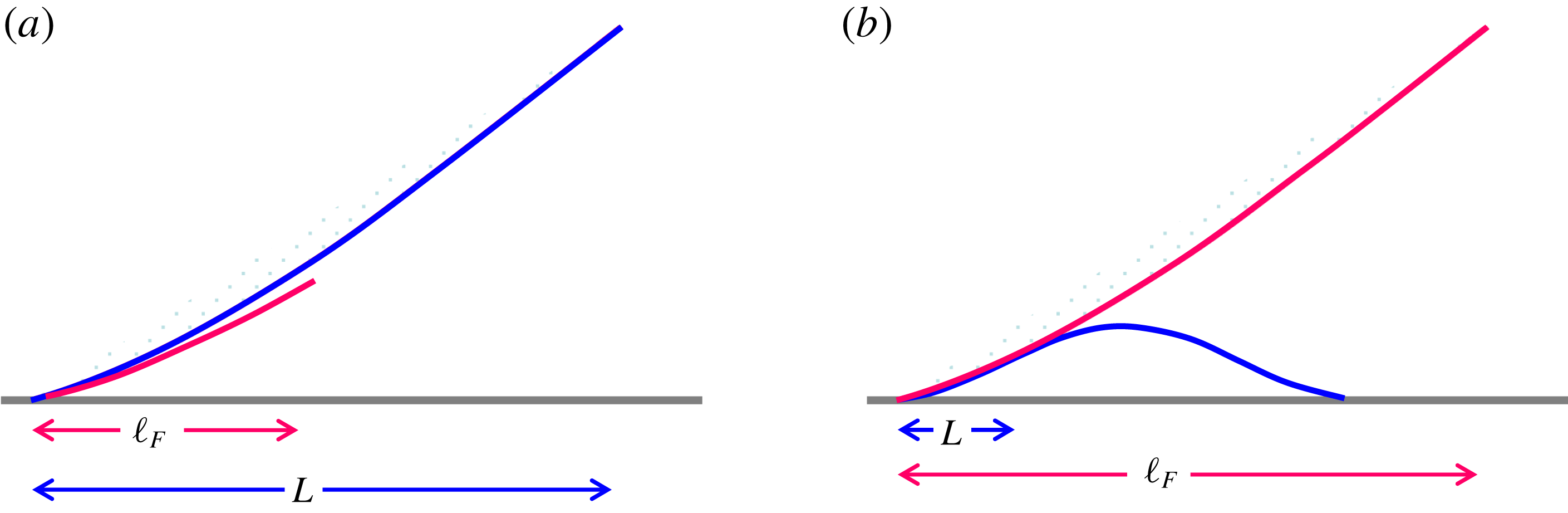
that enters as the outer scale. Figure 3 provides schematics for illustrating how
 $\ell _{F}$
becomes an inner or outer scale with respect to
 $L$
in the determination of
 $\unicode[STIX]{x1D703}_{d}$
.
A schematic illustration of how the extent of slip is determined by the slipping ‘foot’ of width
 $\ell _{F}\sim \unicode[STIX]{x1D706}Ca^{-1/3}$
relative to the macroscopic length
 $L$
: (a)
 $\ell _{F}\ll L$
indicates weak slip, whereas (b)
 $\ell _{F}\gg L$
signifies strong slip.

Finally, we add a remark on the logarithmic terms seen in (4.10) and (4.11). These terms appear at leading order in the dynamic contact angle expressions and diverge as
 $x\rightarrow 0$
. They basically come from an integration of the viscous stress over a wedge-like geometry near the contact line (Voinov Reference Voinov1976; Snoeijer Reference Snoeijer2006). It is worth mentioning that in the works by Lacey (Reference Lacey1982) and Hocking (Reference Hocking1983), a similar logarithmic term was also found but not at leading order. Specifically, this result was obtained by taking a small slip expansion with respect to the quasi-static drop profile that was taken as leading order – it is an outer asymptotic analysis for the motion of a slightly slipping drop. But if taking an inner expansion for this outer problem at the edge of the drop, the diverging terms would be of the same order within the overlap region where inner and outer solutions match (Sibley, Nold & Kalliadasis Reference Sibley, Nold and Kalliadasis2015). Similar appearances of logarithmic terms in the outer and inner regions can also occur when solving the problem in small
 $Ca$
expansion (Cox Reference Cox1986; Hocking Reference Hocking1992; Eggers Reference Eggers2005b
; Bonn et al.
Reference Bonn, Eggers, Indekeu, Meunier and Rolley2009).
5 Impacts of wall slip on dynamic contact angle: model and simulation
5.1 Results of the local lubrication model
Using (4.8b
) (by neglecting
 $h_{1}^{\prime 3}$
) together with the approximation
 $(h,h_{1},h_{\infty })\approx \unicode[STIX]{x1D703}_{d}\times (x,x_{1},x_{\infty })$
in the two
 $F$
terms, the dynamic contact angle
 $\unicode[STIX]{x1D703}_{d}$
can be evaluated in an iterative manner with the initial value
 $(9Ca)^{1/3}$
until its value converges. Note that while the apparent contact angle is defined in a scale of
 $L$
, we do not need to specify a value for
 $L$
in (4.8b
) because
 $h/3\unicode[STIX]{x1D706}$
,
 $h_{1}/3\unicode[STIX]{x1D706}$
and
 $h_{\infty }/3\unicode[STIX]{x1D706}$
in the
 $F$
terms appear in a purely dimensionless manner. This is consistent with the fact that
 $\unicode[STIX]{x1D703}_{d}$
cannot be a function of the relevant length scales separately but of their ratios. So the fact that the result does not depend on the value of
 $L$
is simply because
 $L$
serves as the reference scale for measuring
 $x$
,
 $x_{1}$
,
 $x_{\infty }$
and
 $\unicode[STIX]{x1D706}$
with respect to
 $L$
, i.e.
 $(z,z_{1},z_{\infty },\unicode[STIX]{x1D6FD})=(x,x_{1},x_{\infty },\unicode[STIX]{x1D706})/L$
. In the actual evaluation we take
 $(z,z_{1},z_{\infty })=(1,\unicode[STIX]{x1D6FD},10)$
. We have also verified that the calculated
 $\unicode[STIX]{x1D703}_{d}$
does not vary significantly with the choice of
 $z$
as long as
 $z$
is kept much larger than
 $z_{1}$
(which is taken
 $O(\unicode[STIX]{x1D6FD})$
or smaller) but much smaller than
 $z_{\infty }$
.
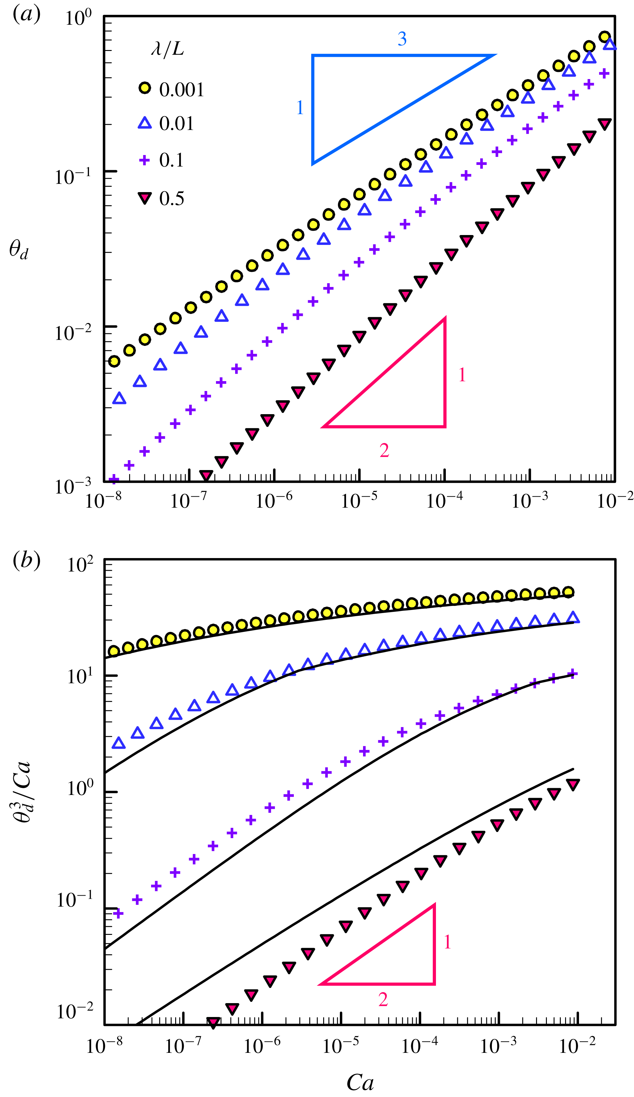
Figure 4(a) plots
 $\unicode[STIX]{x1D703}_{d}$
against
 $Ca$
for different values of
 $\unicode[STIX]{x1D706}/L$
. For a given
 $\unicode[STIX]{x1D706}/L$
,
 $\unicode[STIX]{x1D703}_{d}$
exhibits two distinct behaviours. At
 $\unicode[STIX]{x1D706}/L=0.01$
or smaller,
 $\unicode[STIX]{x1D703}_{d}$
basically follows Tanner’s scaling (2.1):
 $\unicode[STIX]{x1D703}_{d}\sim Ca^{1/3}$
. Increasing
 $\unicode[STIX]{x1D706}$
not only reduces
 $\unicode[STIX]{x1D703}_{d}$
but also gradually changes the dependence of
 $\unicode[STIX]{x1D703}_{d}$
on
 $Ca$
. When increasing
 $\unicode[STIX]{x1D706}/L$
to 0.1 or larger, in particular, the trend shifts to
 $\unicode[STIX]{x1D703}_{d}\propto Ca^{1/2}$
according to the strong-slip scaling (2.4). To better see this transition, figure 4(b) redraws the data by plotting
 $\unicode[STIX]{x1D703}_{d}^{3}/Ca$
against
 $Ca$
. Two distinct trends can be clearly revealed. One appears in the relatively high
 $Ca$
regime (but still
 $\ll 1$
), approaching towards the no-slip limit
 $\unicode[STIX]{x1D703}_{d}^{3}/Ca=\text{const.}$
according to (2.1). The other occurs in the very low
 $Ca$
regime, closely following the strong-slip
 $\unicode[STIX]{x1D703}_{d}^{3}/Ca\propto Ca^{1/2}$
according to (2.4).
(a) Plot of apparent contact angle
 $\unicode[STIX]{x1D703}_{d}$
against
 $Ca$
for various values of
 $\unicode[STIX]{x1D706}/L$
. For a small
 $\unicode[STIX]{x1D706}/L$
like 0.001, the result follows Tanner’s law
 $\unicode[STIX]{x1D703}_{d}\sim Ca^{1/3}$
. Increasing
 $\unicode[STIX]{x1D706}/L$
tends to shift towards the strong-slip law
 $\unicode[STIX]{x1D703}_{d}\propto Ca^{1/2}$
, as indicated by the result of
 $\unicode[STIX]{x1D706}/L=0.5$
. (b) The two distinct trends can be clearly seen by redrawing the data by plotting
 $\unicode[STIX]{x1D703}_{d}^{3}/Ca$
against
 $Ca$
. The solid lines are the approximate results given by (5.1).

Further guided by the two limiting results (4.10b ) and (4.11b ), we find that (4.8b ) can be well approximated by
 $$\begin{eqnarray}\unicode[STIX]{x1D703}_{d}^{3}\approx 9Ca[F(kx_{1}/3\unicode[STIX]{x1D706},kx_{\infty }/3\unicode[STIX]{x1D706})-F(kx/3\unicode[STIX]{x1D706},kx_{\infty }/3\unicode[STIX]{x1D706})],\end{eqnarray}$$
where
 $k$
is the crude value of the asymptotic contact angle taken from (4.10b
) and (4.11b
) separated at
 $Ca=Ca^{\ast }$
due to (4.3):
 $$\begin{eqnarray}k=\left\{\begin{array}{@{}ll@{}}(9Ca)^{1/3} & \text{for }Ca>(L/3\unicode[STIX]{x1D706})^{3}\\ (3Ca)^{1/2}(L/\unicode[STIX]{x1D706})^{1/2} & \text{for }Ca<(L/3\unicode[STIX]{x1D706})^{3}.\end{array}\right.\end{eqnarray}$$
As shown in figure 4(b), (5.1) can fairly capture the results calculated from (4.8b ).
In fact, there is a much simpler way to express
 $\unicode[STIX]{x1D703}_{d}(Ca,\unicode[STIX]{x1D706}/L)$
by lumping both weak-slip and strong-slip results together. Because wall slip tends to reduce viscous drag by a factor
 $h/(h+3\unicode[STIX]{x1D706})$
(where the factor 3 accounts for pressure-driven flow), the effects are equivalent to treating the fluid having an effective viscosity (Liao et al.
Reference Liao, Li and Wei2013; Li et al.
Reference Li, Liao, Wen and Wei2014)
 $$\begin{eqnarray}\unicode[STIX]{x1D702}_{eff}\equiv \unicode[STIX]{x1D702}\left(\frac{1}{3\unicode[STIX]{x1D706}/h+1}\right)\sim \unicode[STIX]{x1D702}\left(\frac{1}{3\unicode[STIX]{x1D706}/L\unicode[STIX]{x1D703}_{d}+1}\right).\end{eqnarray}$$
With
 $\unicode[STIX]{x1D702}_{eff}$
defined by (5.2), the contact line would move as if there were no slip, allowing
 $\unicode[STIX]{x1D703}_{d}$
to be described by the effective Tanner law in terms of the effective capillary number
 $Ca_{eff}=\unicode[STIX]{x1D702}_{eff}U/\unicode[STIX]{x1D6FE}$
:
 $$\begin{eqnarray}\unicode[STIX]{x1D703}_{d}^{3}\sim Ca_{eff}\equiv Ca\left(\frac{1}{3\unicode[STIX]{x1D706}/L\unicode[STIX]{x1D703}_{d}+1}\right).\end{eqnarray}$$
With (5.3), it can be seen quite clearly that small and large
 $\unicode[STIX]{x1D706}/L\unicode[STIX]{x1D703}_{d}$
recover the weak-slip scaling (2.1),
 $\unicode[STIX]{x1D703}_{d}\sim Ca^{1/3}$
, and the strong-slip scaling (2.4),
 $\unicode[STIX]{x1D703}_{d}\sim Ca^{1/2}(L/\unicode[STIX]{x1D706})^{1/2}$
, respectively. The crossover (2.3),
 $Ca^{\ast }\sim (\unicode[STIX]{x1D706}/L)^{3}$
, can also be readily obtained by setting
 $\unicode[STIX]{x1D706}/L\unicode[STIX]{x1D703}_{d}\sim O(1)$
and
 $\unicode[STIX]{x1D703}_{d}\sim Ca^{1/3}$
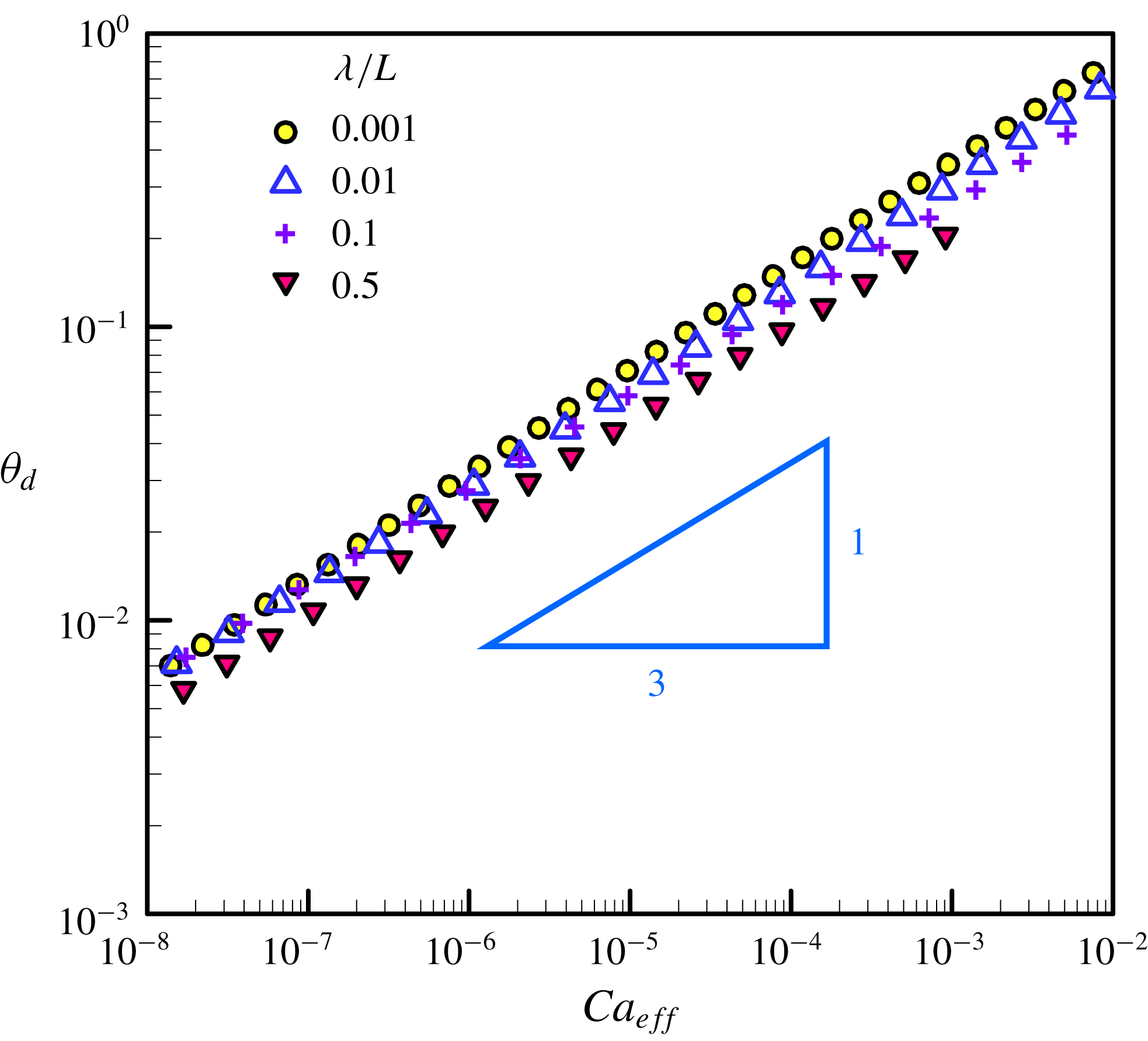
in (5.3). As shown in figure 5, all the data with different values of
 $\unicode[STIX]{x1D706}/L$
seen in figure 4(a) can be successfully collapsed according to (5.3), confirming the notions of the effective viscosity (5.2) discussed above.
Replot of the data in figure 4(a) by plotting
 $\unicode[STIX]{x1D703}_{d}$
against the effective capillary number
 $Ca_{eff}=\unicode[STIX]{x1D702}_{eff}U/\unicode[STIX]{x1D6FE}$
defined by (5.3). The data with different values of slip length can be collapsed according to the effective Tanner law:
 $\unicode[STIX]{x1D703}_{d}\sim Ca_{eff}^{1/3}$
.

5.2 Issues involved in resolving the motion of a slipping contact line
The results presented above are based on the approximate solution (4.8) to the local equation (4.2). It may be tempting to verify the former by solving the latter directly. However, this is not a self-contained procedure because the yet-to-be-determined dynamic contact angle itself has to be specified as part of the boundary conditions needed for solving the equation. In fact, there are more reasons why a complete dynamic contact angle relationship generally cannot be fully resolved by doing such.
First of all, (4.8) is a local solution that requires to match the outer macroscopic region away from the contact line. How the influence of macroscopic features enters the contact line dynamics manifests by the fact that the apparent dynamic contact angle
 $\unicode[STIX]{x1D703}_{d}\equiv h^{\prime }(x=L)$
is often evaluated at the inflection point at which the wedge-like interface starts to decrease its slope in the direction towards the central cap of a spreading droplet (Kavehpour et al.
Reference Kavehpour, Ovryn and McKinley2003; Pahlavan et al.
Reference Pahlavan, Cueto-Felgueroso, McKinley and Juanes2015). Because of the cap,
 $L=cR$
has to be connected to the spreading radius
 $R$
through a constant
 $c$
that will be determined by matching the solution to the outer cap region. In other words, the actual dynamic contact angle relationship generally involves
 $R$
.
Second, whether the physics of a moving contact line can be well decoupled from the outer drop depends on whether the relevant length scales are well separated. For no-slip or weak-slip case where
 $\unicode[STIX]{x1D706}\ll h$
,
 $h^{2}h^{\prime \prime \prime }=-3Ca$
reduced from (3.6) has a solution form
 $h=LCa^{1/3}H(x/L)$
which is invariant of
 $L$
(Bonn et al.
Reference Bonn, Eggers, Indekeu, Meunier and Rolley2009). This scale invariance allows
 $L$
to be taken to be any value below
 $R$
without changing
 $\unicode[STIX]{x1D703}_{d}$
. In other words, the form of (4.10b
) is universal (Bonn et al.
Reference Bonn, Eggers, Indekeu, Meunier and Rolley2009), determined mainly by the local hydrodynamics near the contact line. In this case, the impact from the outer drop through
 $x\rightarrow cR$
only enters the logarithmic factor and hence does not affect the contact line characteristics qualitatively. If
 $\unicode[STIX]{x1D706}$
becomes comparable to or greater than
 $h$
, however, the requirement of
 $\unicode[STIX]{x1D706}$
in the solution to (3.6) necessitates
 $L$
to enter the solution in the form of
 $h=\unicode[STIX]{x1D706}H(x/L,Ca(L/\unicode[STIX]{x1D706})^{3})$
. The need to fix the solution by specifying
 $L$
through matching to the outer drop means that the local solution is no longer separated from that of the drop. So the dynamic contact angle has to be determined by all the length scales involved, as also indicated by (4.8b
) or (4.11b
).
In addition, (4.8b
) also involves the microscopic length
 $x_{1}$
, which needs to be sought from the inner region of the contact line. Therefore, a complete description of the dynamic contact angle requires matching to both the inner and outer regions by specifying
 $x_{1}$
and
 $L$
(or
 $x_{\infty }$
). In the case of
 $\unicode[STIX]{x1D706}\ll h$
, (4.10b
) can be tested by solving the local equation (4.2) with
 $x_{1}$
that can be found by the inner solution of (4.2) (Eggers Reference Eggers2005b
) or by including the additional disjoining pressure term (Hervet & de Gennes Reference Hervet and de Gennes1984; Eggers & Stone Reference Eggers and Stone2004; see also § 6.5) without having to specify
 $L$
. In the latter case, (4.11b
) dominates the inner region but still requires
 $x_{\infty }$
to be determined by matching to (4.10b
) (see § 6.5). But if
 $\unicode[STIX]{x1D706}$
is comparable to or greater than
 $h$
, because there will be no clear cut between the ‘foot’ and the central cap (see §§ 4.2 and 4.3), to find
 $L$
or
 $x_{\infty }$
it is necessary to solve the outer drop. In one way or another, one has to either match or couple to the outer drop. So if one wishes to fully test how wall slip affects the dynamic contact angle, one might still have to resort to solving the entire drop spreading problem.
5.3 Many-body dissipative particle dynamics simulations
Numerically simulating a drop spreading problem is commonly realized by solving a time-dependent hydrodynamic equation. Similar to the situation in solving (4.2), solving such an equation still requires boundary conditions at the contact line, and one of which has to specify the dynamic contact angle that is actually part of the solution needed to be determined. It is possible to determine the apparent dynamic contact angle through the inflection point by setting a vanishing slope or interfacial tension at the edge of a spreading drop (Pahlavan et al. Reference Pahlavan, Cueto-Felgueroso, McKinley and Juanes2015). But it has to be implemented at the expense of the inclusion of microscopic intermolecular forces for advancing the contact line. As a result, the problem will involve many disparate length scales, making its numerical computation prohibitively expensive (Pahlavan et al. Reference Pahlavan, Cueto-Felgueroso, McKinley and Juanes2015).
To avoid the issues mentioned above, an alternative approach is needed. Here we choose the many-body dissipative particle dynamics (MDPD) to test our theory. The main advantage of MDPD is that it does not require the imposition of boundary conditions at the contact line. Moreover, this approach allows us to simulate spreading of nanodroplets to which impacts of wall slip can be made more pronounced. The simulation method basically follows Weng et al. (Reference Weng, Wu, Tsao and Sheng2017) with slight modifications by allowing fluid slippage on the solid surface. The simulations are performed in a box with a size of
 $80\times 80\times 80$
in units of the bead radius
 $r_{bead}$
. The total bead number of the liquid is 30 000. In each simulation, a drop begins with a perfect sphere having contact angle
 $\unicode[STIX]{x1D703}_{d}=180^{\circ }$
. Changes in
 $\unicode[STIX]{x1D703}_{d}$
can be observed when the base radius
 $R$
reaches
 $10r_{bead}$
or greater. Time
 $t$
is measured in terms of the number of time steps
 $t_{step}=0.01t_{bead}$
, where
 $t_{bead}=r_{bead}/v_{rms}$
is based on the root-mean-square velocity
 $v_{rms}=(3k_{B}T/m)^{1/2}$
in terms of the thermal energy
 $k_{B}T$
and the bead mass
 $m$
.
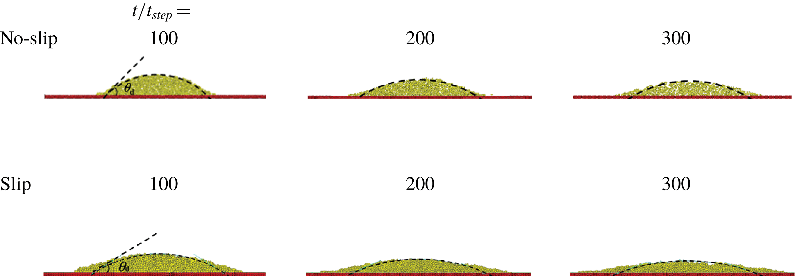
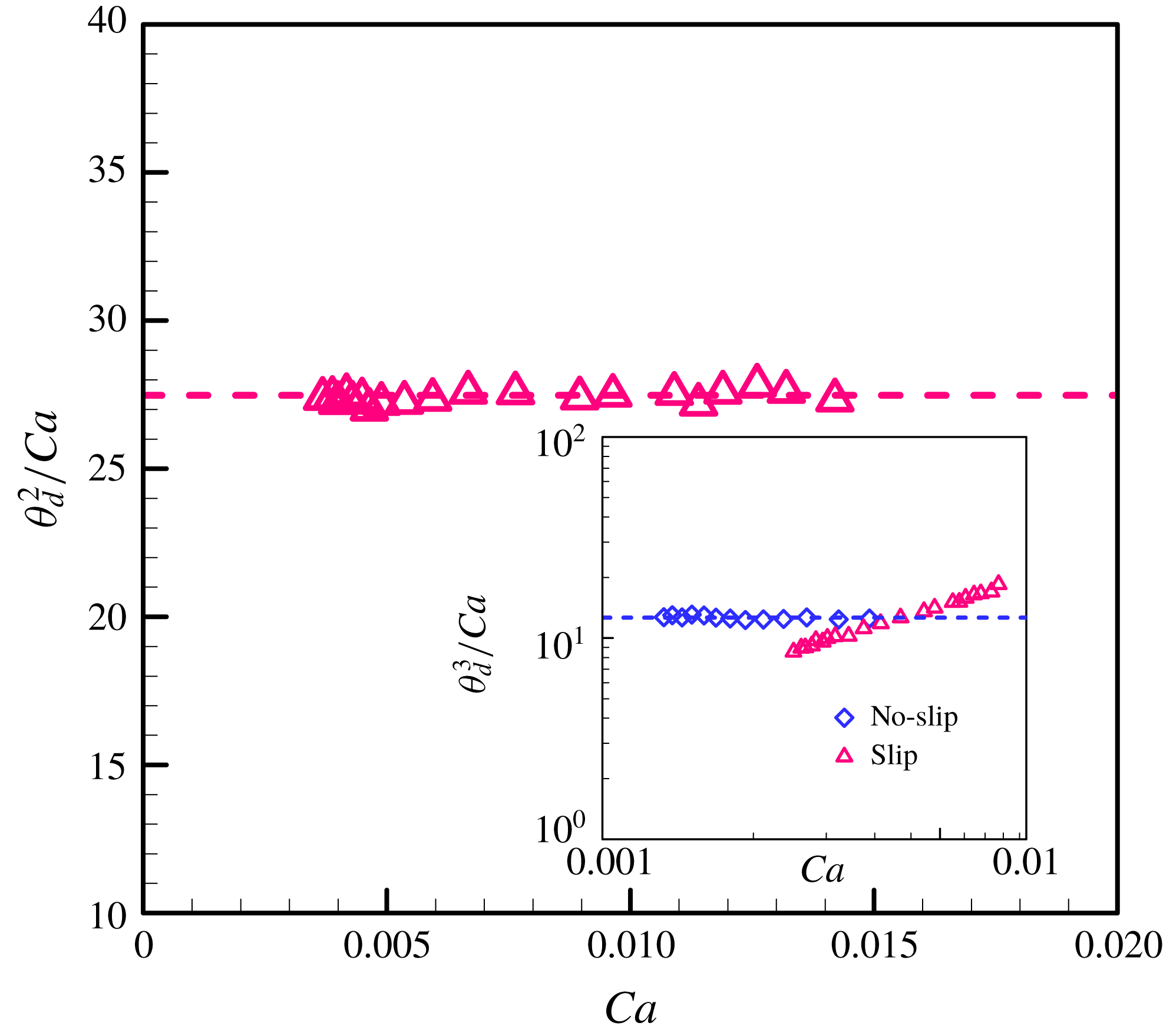
Figure 6 displays snapshots of nanodrop spreading with and without slip, showing that the drop with slip spreads faster than that without slip. Figure 7 plots the rescaled dynamic contact angle
 $\unicode[STIX]{x1D703}_{d}^{2}/Ca$
against
 $Ca$
for the slip case. It clearly shows
 $\unicode[STIX]{x1D703}_{d}^{2}/Ca=\text{const}.$
, which successfully captures the strong-slip law (2.4). The inset also shows
 $\unicode[STIX]{x1D703}_{d}^{3}/Ca=\text{const}.$
for the no-slip case, confirming Tanner’s law (2.1) as well.
Some snapshots using MDPD simulations for nanodrop spreading with and without slip. The results clearly show that slip can make a drop spread faster. In the case of slip, the slip length is taken as
 $\unicode[STIX]{x1D706}=3.14r_{bead}$
greater than the liquid height
 $h$
, where
 $r_{bead}$
is the bead radius. In either case, the drop begins with a perfect sphere of identical radius and contact angle
 $\unicode[STIX]{x1D703}_{d}=180^{\circ }$
. Changes in
 $\unicode[STIX]{x1D703}_{d}$
can be observed when the base radius
 $R$
reaches
 $10r_{bead}$
or greater. Time
 $t$
is expressed as the number of time steps
 $t_{step}=0.01t_{bead}$
, where
 $t_{bead}=r_{bead}/v_{rms}$
is the characteristic time based on the root-mean-square velocity
 $v_{rms}=(3k_{B}T/m)^{1/2}$
with
 $k_{B}T$
being the thermal energy and
 $m$
the bead mass.

Plot of the rescaled apparent dynamic contact angle
 $\unicode[STIX]{x1D703}_{d}^{2}/Ca$
against
 $Ca$
for the slip case seen in figure 6. The result clearly reveals
 $\unicode[STIX]{x1D703}_{d}^{2}/Ca=\text{const.}$
, successfully capturing the strong-slip scaling (2.4). The inset plots
 $\unicode[STIX]{x1D703}_{d}^{3}/Ca$
against
 $Ca$
, showing that
 $\unicode[STIX]{x1D703}_{d}^{3}/Ca=\text{const.}$
for the no-slip case, which also confirms Tanner’s law (2.1) as well. The dashed lines in these plots represent best fits.

Chan et al. (Reference Chan, McGraw, Salez, Seemann and Brinkmann2017) found in their simulations that a dewetting drop on a slippery surface can display a non-spherical shape due to slip effects. In contrast to their study, we do not observe significant departures from spherical drop shape for the slip case. The reasons are: (i) the drop is very small and (ii) we look at the complete wetting scenario where the contact angle is small and constantly decreasing during spreading. Although in our case the ‘foot’ may come into play to make the interface deviate from spherical shape, the changes of the interface curvature are actually not noticeable because of the above reasons. This is also consistent with the consequence of the small-slope theory we use in our analysis.
We notice that there are two important differences between our work and that of Chan et al.: (i) our focus is wetting whereas that of Chan et al. is dewetting and (ii) our contact angle is of advancing type and constantly decreasing, whereas theirs is of receding type but kept fixed at the equilibrium value. Because their drop is getting thicker as it retracts, the asphericity in their drop shape might be a result of the necessary adjustment of the interface for matching the constant contact angle set at the drop edge. In contrast, in our case the drop is getting thinner as it spreads, making the interface curvature gradually diminish. Obviously, their interface adjustment is much more pronounced than ours, explaining why apparent asphericity in the drop shape can be observed in their work but not in the present study. It is also worth mentioning that apparent changes in interface profiles can arise purely from very large slip beyond (3.7), as shown by Münch et al. (Reference Münch, Wagner and Witelski2005) in their study on dewetting films without contact lines. Such changes come from the strong coupling between slip and inertial effects (Münch et al. Reference Münch, Wagner and Witelski2005), which is beyond the scope of the present work.
To capture the interface adjustment due to wall slip, which manifests most near the contact line, we will further include the van der Waals disjoining pressure in § 6 to numerically resolve the interface profile in the vicinity of the contact line. As will be shown in § 6.5, for a weakly slipping drop whose contact line structure involves both Tanner’s law (4.10b ) and the strong-slip law (4.11b ), the interface profile can be precisely portrayed by these two laws by solving (6.2) numerically. More importantly, we will reveal that a ‘foot’ will naturally form from a strongly slipping precursor film.
6 Decoding the microstructure of a slipping contact line
6.1 Motivation and problem set-up
As for the microscopic characteristics of a moving contact line, they are usually determined by either wall slip or disjoining pressure (Eggers & Stone Reference Eggers and Stone2004), and each is considered as a separate microscopic mechanism for removing the contact line stress singularity. In the case of a polymer liquid in which slip effects may be strong, both slip and disjoining pressure effects might have to be considered jointly. This might lead the precursor film to behave differently from that without slip described by Hervet & de Gennes (Reference Hervet and de Gennes1984).
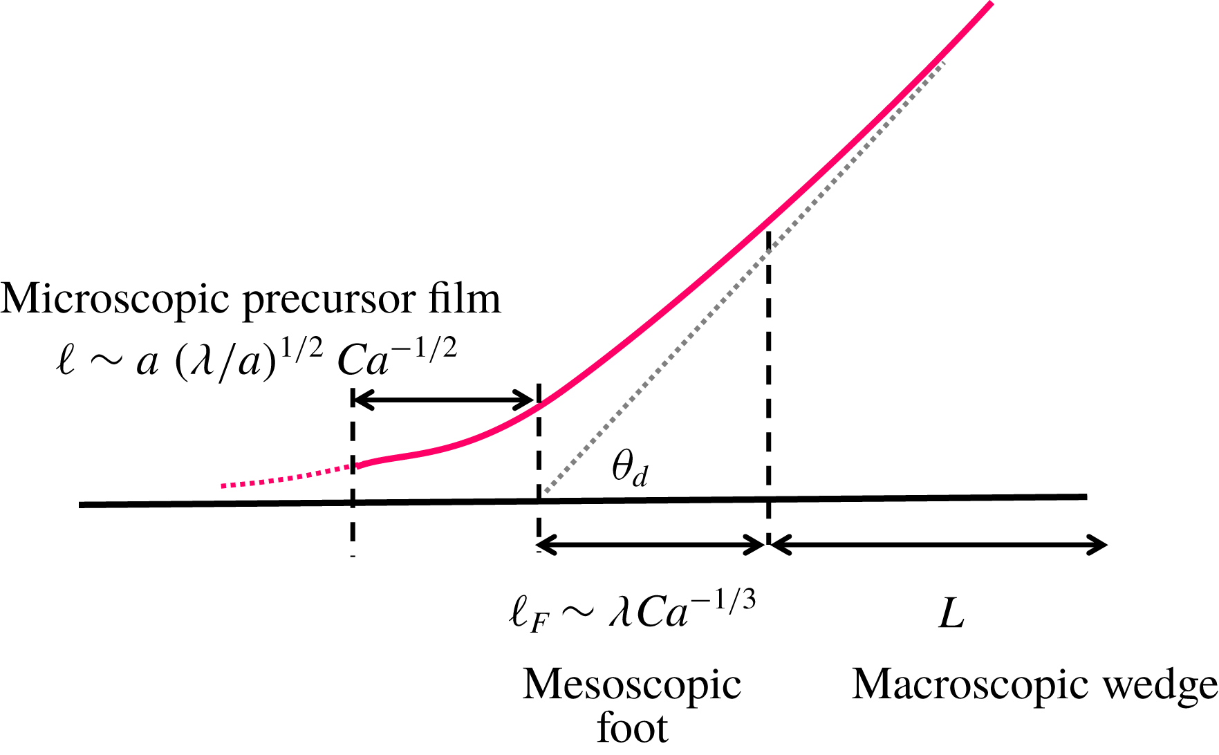
In fact, even though the slip length is macroscopically small, it could still be microscopically large to cause substantial impacts on the microscopic behaviour of a moving contact line. This case actually occurs to a thick polymer drop in which the slip length is much smaller than the drop height but much greater than the precursor film. It has been reported that the simple slip model (3.6) can give a microscopic ‘foot’ length (2.5) in the logarithmic factor of the Tanner–Cox–Voinov law (4.10b ) (Hocking Reference Hocking1983, Reference Hocking1992; Eggers & Stone Reference Eggers and Stone2004). In contrast, if disjoining pressure is taken into account without slip, the width of the precursor film will become the microscopic length (Hervet & de Gennes Reference Hervet and de Gennes1984; Eggers & Stone Reference Eggers and Stone2004). If both slip and disjoining pressure coexist as occurring for polymer liquids, it is not clear whether the microscopic length is still dictated by the precursor film.
It is worth mentioning that Brochard & de Gennes (Reference Brochard and de Gennes1984) have analysed the spreading of a polymer drop by including both wall slip and disjoining pressure. They mainly focused on the formation of the mesoscopic ‘foot’ behind the precursor film. They also considered effects of wall slip on the interface profile of the precursor film, and merely obtained the ‘maximal’ film profile by balancing viscous force to disjoining pressure force. However, how this maximal film develops into the ‘foot’, which has to further take into account surface tension force, was not addressed in their study.
In view of the above, while most existing studies have used either wall slip or disjoining pressure in resolving the microscopic behaviour of a moving contact line (Hervet & de Gennes Reference Hervet and de Gennes1984; Kalliadasis & Chang Reference Kalliadasis and Chang1996; Eggers Reference Eggers2004; Eggers & Stone Reference Eggers and Stone2004; Eggers Reference Eggers2005a ; Savva & Kalliadasis Reference Savva and Kalliadasis2011), there has been no systematic attempt to examine the combined influence of these two effects. While this issue has been briefly discussed by Brochard & de Gennes (Reference Brochard and de Gennes1984) and Liao et al. (Reference Liao, Li and Wei2013), below we develop a new theory to provide a more in-depth analysis for the microstructure of a slipping contact line.
We begin with the van der Waals disjoining pressure:
 $$\begin{eqnarray}\prod =\unicode[STIX]{x1D6FE}\frac{a^{2}}{h^{3}},\end{eqnarray}$$
where
 $a=(A_{H}/6\unicode[STIX]{x03C0}\unicode[STIX]{x1D6FE})^{1/2}$
is the molecular length which is typically of the order of 1 Å and
 $A_{H}$
is the Hamaker constant. The equation governing the precursor film motion can be derived by simply adding
 $-\prod$
from (6.1) to the Laplace pressure (3.2), which modifies (3.6) to
 $$\begin{eqnarray}h^{\prime \prime \prime }=-\frac{3Ca}{h^{2}+3\unicode[STIX]{x1D706}h}+\frac{3a^{2}h^{\prime }}{h^{4}}.\end{eqnarray}$$
The corresponding dimensionless form under (4.1) is
 $$\begin{eqnarray}H^{\prime \prime \prime }=-\frac{3\unicode[STIX]{x1D6FF}}{H^{2}+H}+\frac{3\unicode[STIX]{x1D712}H^{\prime }}{H^{4}},\end{eqnarray}$$
where
 $\unicode[STIX]{x1D712}$
measures the strength of the microscopic disjoining pressure relative to the macroscopic Laplace pressure according to
 $$\begin{eqnarray}\unicode[STIX]{x1D712}=\left(\frac{a}{3\unicode[STIX]{x1D706}}\right)^{2}\left(\frac{L}{3\unicode[STIX]{x1D706}}\right)^{2}.\end{eqnarray}$$
Note that (6.2b
) is derived for length scale
 $z=O(1)$
or
 $x=O(L)$
. Since we are looking at the inner contact line region characterized by the precursor film of thickness
 $h_{f}$
and length
 $\ell$
,
 $H$
and
 $z$
should scale as
 ${\mathcal{H}}=h_{f}/3\unicode[STIX]{x1D706}$
and
 ${\mathcal{L}}=\ell /L$
, respectively. The actual scales for
 ${\mathcal{H}}$
and
 ${\mathcal{L}}$
will be determined by balancing the terms in (6.2b
), and hence those for
 $h_{f}$
and
 $\ell$
.
We first balance the surface tension term
 $H^{\prime \prime \prime }\sim {\mathcal{H}}/{\mathcal{L}}^{3}$
to the disjoining pressure term
 $3\unicode[STIX]{x1D712}H^{\prime }/H^{4}\sim \unicode[STIX]{x1D712}/{\mathcal{H}}^{3}{\mathcal{L}}$
. This yields the scale for the precursor film thickness,
 ${\mathcal{H}}\sim (\unicode[STIX]{x1D712}{\mathcal{L}}^{2})^{1/4}$
, or its dimensional form
 $$\begin{eqnarray}h_{f}\sim (a\ell )^{1/2}.\end{eqnarray}$$
Here the length
 $\ell$
we are looking at is the length of the transition portion of the film bridging towards the macroscopic wedge (de Gennes Reference de Gennes1985), rather than the length of a fully extended film (or called ‘truncated’ film) that is determined by the spreading coefficient (de Gennes Reference de Gennes1985; Colinet & Rednikov Reference Colinet and Rednikov2011). If the drop is not very small and if its spreading merely takes place for a relatively short period after its deposition, the film might not fully thin down to the equilibrium ‘pancake’ state whose thickness is often of molecular size (Beaglehole Reference Beaglehole1989). In this case,
 $\ell$
may represent the majority part of such a gradually developing film whose spreading power is not yet burned at the molecular level. We are in particular interested in
 $\ell$
since it can enter as the microscopic length
 $x_{1}$
in the logarithmic factor of the Tanner–Cox–Voinov law (4.10b
) (de Gennes Reference de Gennes1985; Eggers & Stone Reference Eggers and Stone2004). In addition, it can also impact the spreading kinetics of the film (see § 7.2).
As such,
 $h_{f}$
given by (6.4) should represent the crossover thickness to the ‘maximal’ film (de Gennes Reference de Gennes1985). Because
 $h_{f}$
is typically small and also because
 $\unicode[STIX]{x1D706}$
can vary in a wide range, the actual behaviour of the precursor film must lie between two limiting situations: (i) thick film with
 $h_{f}\gg \unicode[STIX]{x1D706}$
and (ii) thin film with
 $h_{f}\ll \unicode[STIX]{x1D706}$
, which are examined below.
6.2 Thick film with small microscopic slip
For the thick-film case with
 $h_{f}\gg \unicode[STIX]{x1D706}$
, it is the situation where
 $\unicode[STIX]{x1D706}$
is extremely small. Now because
 ${\mathcal{H}}\gg 1$
, the viscous term in (6.2b
) scales as
 $\unicode[STIX]{x1D6FF}/H^{2}\sim \unicode[STIX]{x1D6FF}/{\mathcal{H}}^{2}$
. Balancing the viscous term to the surface tension term,
 $\unicode[STIX]{x1D6FF}/{\mathcal{H}}^{2}\sim {\mathcal{H}}/{\mathcal{L}}^{3}$
, together with (6.4), we arrive at
 ${\mathcal{L}}\sim \unicode[STIX]{x1D712}^{1/2}\unicode[STIX]{x1D6FF}^{-2/3}$
, which recovers the no-slip precursor film scaling (Hervet & de Gennes Reference Hervet and de Gennes1984; Eggers & Stone Reference Eggers and Stone2004):
 $$\begin{eqnarray}\ell \sim aCa^{-2/3}.\end{eqnarray}$$
Substitution of (6.5) into (6.4) gives the corresponding film thickness scale:
 $$\begin{eqnarray}h_{f}\sim aCa^{-1/3}.\end{eqnarray}$$
This thick film situation requires
 $h_{f}\gg \unicode[STIX]{x1D706}$
, yielding
 $$\begin{eqnarray}\frac{\unicode[STIX]{x1D706}}{a}\ll Ca^{-1/3},\end{eqnarray}$$
under which (6.5) and (6.6) characterize the film dimensions. In terms of the spreading kinetics, (6.5) suggests that the film will extend its length with time according to
 $$\begin{eqnarray}\ell \sim a(\unicode[STIX]{x1D6FE}t/\unicode[STIX]{x1D702}a)^{2/5}.\end{eqnarray}$$
6.3 Thin film with large microscopic slip
When the film is thin such that
 $h_{f}\ll \unicode[STIX]{x1D706}$
, the film will experience a large microscopic slip, which is likely the case for polymer liquids. Since
 ${\mathcal{H}}\ll 1$
, the viscous term in (6.2b
),
 $-3\unicode[STIX]{x1D6FF}/(H^{2}+H)$
, scales as
 $\unicode[STIX]{x1D6FF}/H\sim \unicode[STIX]{x1D6FF}/{\mathcal{H}}$
dominated by the slip term. Balancing
 $\unicode[STIX]{x1D6FF}/{\mathcal{H}}$
to the surface tension term
 $H^{\prime \prime \prime }\sim {\mathcal{H}}/{\mathcal{L}}^{3}$
and using (6.4), we find
 ${\mathcal{L}}\sim (\unicode[STIX]{x1D712}/\unicode[STIX]{x1D6FF}^{2})^{1/4}$
whose dimensional form reads
 $$\begin{eqnarray}\ell \sim a(\unicode[STIX]{x1D706}/a)^{1/2}Ca^{-1/2}.\end{eqnarray}$$
Expression (6.9) indicates that the larger the value of
 $\unicode[STIX]{x1D706}$
the longer the film because its advancement is promoted by slip. The corresponding film thickness can be obtained by substituting (6.9) into (6.4):
 $$\begin{eqnarray}h_{f}\sim a(\unicode[STIX]{x1D706}/a)^{1/4}Ca^{-1/4}.\end{eqnarray}$$
Because
 $h_{f}\ll \unicode[STIX]{x1D706}$
here, this together with (6.10) gives
 $$\begin{eqnarray}\frac{\unicode[STIX]{x1D706}}{a}\gg Ca^{-1/3},\end{eqnarray}$$
under which both (6.9) and (6.10) hold for this thin-film situation.
The film thickness scale (6.10) indicates that wall slip tends to thicken the film. This can be seen by comparing the strong-slip case to the weak-slip case. Because of (6.11), the film thickness (6.10) for the former is a factor
 $[(\unicode[STIX]{x1D706}/a)Ca^{1/3}]^{1/4}(\gg 1)$
thicker than (6.6) for the latter.
Finally, in terms of the film spreading kinetics, the spreading law corresponding to (6.9) is
 $$\begin{eqnarray}\ell \sim a(\unicode[STIX]{x1D706}/a)^{1/3}(\unicode[STIX]{x1D6FE}t/\unicode[STIX]{x1D702}a)^{1/3}.\end{eqnarray}$$
The resulting spreading exponent is
 $1/3$
, smaller than the
 $2/5$
of the weak-slip case (6.8).
6.4 Classification of contact line structures
As shown above, the precursor film can display either the thin-film scales (6.9)–(6.10) or the thick-film scales (6.5)–(6.6), depending on
 $(\unicode[STIX]{x1D706}/a)Ca^{1/3}$
according to (6.7) or (6.11). Recall that the extent of slip at the macroscopic level is determined by the ‘foot’ size
 $\unicode[STIX]{x1D706}Ca^{-1/3}$
relative to
 $L$
according to (4.3). Even though slip may be microscopically strong with
 $(\unicode[STIX]{x1D706}/a)Ca^{1/3}>1$
, its amount is not necessarily large at the macroscopic level because
 $(\unicode[STIX]{x1D706}/L)Ca^{-1/3}$
could be small.
To better identify the parameter regimes in which slip effects are important at the macroscopic or/and microscopic levels, the situation can be categorized in terms of ‘thick/thin drop’ and ‘thick/thin film’. The former represents ‘weak/strong macroscopic slip’ using
 $\unicode[STIX]{x1D6FF}$
defined by (4.3), whereas the latter signifies ‘small/large microscopic slip’ according to (6.7)/(6.11). As illustrated in figure 8, there exist three types of contact line structures: (i) thick drop with thin film, (ii) thick drop with thick film and (iii) thin drop with thick film, depending on the value of
 $Ca$
with respect to
 $(\unicode[STIX]{x1D706}/L)^{3}$
and
 $(\unicode[STIX]{x1D706}/a)^{-3}$
.
A diagram that illustrates possible macroscopic and microscopic structures of a moving contact line in terms of
 $Ca$
and the strength of wall slip. The situation can be categorized in terms of ‘thick/thin drop’ representing ‘weak/strong macroscopic slip’ as well as ‘thin/thick film’ signifying ‘large/small microscopic slip’, depending on the value of
 $Ca$
with respect to
 $(\unicode[STIX]{x1D706}/L)^{3}$
and
 $(\unicode[STIX]{x1D706}/a)^{-3}$
. Even though slip effects are macroscopically weak in ‘thick drop’ under
 $Ca\,(L/\unicode[STIX]{x1D706})^{3}>1$
, the microscopic contact line structure can still be well characterized by ‘thin film’ having large microscopic slip under
 $Ca\,(\unicode[STIX]{x1D706}/a)^{3}>1$
, as illustrated on the top-right corner.

Figure 8 clearly reveals that even though slip effects are macroscopically weak for ‘thick drop’ under
 $\unicode[STIX]{x1D706}/L\ll Ca^{1/3}$
, the microscopic contact line can still be well characterized by ‘thin film’ having large microscopic slip under
 $\unicode[STIX]{x1D706}/a\gg Ca^{-1/3}$
. The two conditions above give the range of the slip length
 $\unicode[STIX]{x1D706}$
for such thick-drop and thin-film situation:
 $$\begin{eqnarray}1\ll (\unicode[STIX]{x1D706}/a)Ca^{1/3}\ll (L/a)Ca^{2/3}.\end{eqnarray}$$
Recall (6.7) or (6.11) that
 $(\unicode[STIX]{x1D706}/a)\,Ca^{1/3}$
measures the extent of microscopic slip. With
 $a\sim 0.1~\text{nm}$
and
 $Ca$
typically
 ${\geqslant}10^{-6}$
, slip will start to become microscopically large for
 $\unicode[STIX]{x1D706}>10~\text{nm}$
. For polymer liquids, in particular,
 $\unicode[STIX]{x1D706}$
is of the order of micrometres or larger. So
 $(\unicode[STIX]{x1D706}/a)\,Ca^{1/3}$
is at least
 $O(10^{2})$
. In this case, to ensure that slip can be made macroscopically small using a sufficiently thick drop under
 $\unicode[STIX]{x1D706}/L<Ca^{1/3}$
, the drop size
 ${\sim}L$
has to be at least
 $10^{2}~\unicode[STIX]{x03BC}\text{m}$
or larger.
In fact, (6.13) is automatically satisfied if
 $Ca^{1/3}\gg (\unicode[STIX]{x1D706}/a)^{-1}\gg \unicode[STIX]{x1D706}/L$
. The inequality between the latter two yields
 $$\begin{eqnarray}\unicode[STIX]{x1D706}^{2}/aL\ll 1.\end{eqnarray}$$
Expression (6.14) is essentially
 $\unicode[STIX]{x1D712}\gg 1$
in (6.2b
), meaning that the microscopic disjoining pressure has to outweigh the macroscopic Laplace pressure. Note that for the thick film case with
 $(\unicode[STIX]{x1D706}/a)^{-1}\gg Ca^{1/3}\gg \unicode[STIX]{x1D706}/L$
, (6.14) also holds. But this case may not show up in the microstructure of the contact line unless
 $\unicode[STIX]{x1D706}$
is extremely small such that
 $\unicode[STIX]{x1D706}^{2}/aL\ll (\unicode[STIX]{x1D706}/a)Ca^{1/3}\ll 1$
. For polymer drops with
 $L\sim 1~\text{mm}$
,
 $\unicode[STIX]{x1D706}\sim 1~\unicode[STIX]{x03BC}\text{m}$
and
 $a\sim 0.1~\text{nm}$
, (6.14) is always satisfied. Also given that
 $Ca$
is typically
 ${\geqslant}10^{-6}$
much greater than
 $(\unicode[STIX]{x1D706}/a)^{-3}\sim 10^{-12}$
according to (6.11), the thin-film scalings (6.9)–(6.10) should enter the microstructure of the contact line for a polymer drop. Hence, the no-slip precursor film model developed by Hervet & de Gennes (Reference Hervet and de Gennes1984) might not be an adequate description for the precursor film of a polymer drop. There are a few experimental studies that support this view, as will be shown in § 7.2.
6.5 Bridging thin film to thick drop
As discussed above, a thick drop having small macroscopic slip may perceive a large microscopic slip in the vicinity of the contact line. While the wetting dynamics of the drop can be described by the Tanner–Cox–Voinov law (4.10b
), the description cannot be said to be complete without specifying the inner length
 $x_{1}$
, which is determined by the specific features of the microscopic contact line. This not only requires one to solve (6.2a
) for resolving the inner interface profile, but also necessitates matching of the solution to (4.10b
) away from the contact line.
To solve (6.2a
), we rescale the variables as
 $(\unicode[STIX]{x1D719},\unicode[STIX]{x1D709})=(h/h_{f},x/\ell )$
using the thin-film scales (6.9)–(6.10) under
 $\unicode[STIX]{x1D6EC}\equiv (\unicode[STIX]{x1D706}/a)Ca^{1/3}\gg 1$
. This transforms (6.2a
) to
 $$\begin{eqnarray}\unicode[STIX]{x1D719}^{\prime \prime \prime }=-\frac{1}{\unicode[STIX]{x1D6FF}_{1}\unicode[STIX]{x1D719}^{2}+\unicode[STIX]{x1D719}}+\frac{3\unicode[STIX]{x1D719}^{\prime }}{\unicode[STIX]{x1D719}^{4}},\end{eqnarray}$$
where the dimensionless parameter
 $\unicode[STIX]{x1D6FF}_{1}$
is
 $$\begin{eqnarray}\unicode[STIX]{x1D6FF}_{1}\equiv \frac{h_{f}}{3\unicode[STIX]{x1D706}}=\frac{1}{3}\unicode[STIX]{x1D6EC}^{-3/4}=\frac{1}{3}\left(\frac{\unicode[STIX]{x1D706}}{a}Ca^{1/3}\right)^{-3/4}.\end{eqnarray}$$
So the extent of microscopic slip can be reflected by
 $1/\unicode[STIX]{x1D6FF}_{1}$
. Here we are more interested in the large microscopic slip case
 $\unicode[STIX]{x1D6FF}_{1}\ll 1$
(but restrict its value to be much larger than
 $[(L/a)Ca^{2/3}]^{-3/4}$
according to (6.13) to ensure weak macroscopic slip).
To solve (6.15) numerically, we follow the approach of Hervet & de Gennes (Reference Hervet and de Gennes1984) or of Eggers & Stone (Reference Eggers and Stone2004). We first construct an approximate profile
 $\unicode[STIX]{x1D719}^{{<}}$
for
 $\unicode[STIX]{x1D719}(\unicode[STIX]{x1D709}<0)$
ahead of the macroscopic contact line at
 $\unicode[STIX]{x1D709}=0$
, and then use it to integrate (6.15) towards
 $\unicode[STIX]{x1D709}>0$
with a vanishing curvature as
 $\unicode[STIX]{x1D709}\rightarrow \infty$
. An appropriate form of
 $\unicode[STIX]{x1D719}^{{<}}$
, first of all, has to follow the asymptote
 $\unicode[STIX]{x1D719}(\unicode[STIX]{x1D709}\rightarrow -\infty )\equiv \unicode[STIX]{x1D719}_{0}$
, called the ‘maximal film’. Here
 $\unicode[STIX]{x1D719}_{0}$
can be determined by considering only the slip part
 $-1/\unicode[STIX]{x1D719}$
of the viscous term (since
 $\unicode[STIX]{x1D719}\gg \unicode[STIX]{x1D6FF}_{1}\unicode[STIX]{x1D719}^{2}$
as
 $\unicode[STIX]{x1D719}(\unicode[STIX]{x1D709}\rightarrow -\infty )\rightarrow 0$
) and the disjoining pressure term
 $3\unicode[STIX]{x1D719}^{\prime }/\unicode[STIX]{x1D719}^{4}$
in (6.15):
 $$\begin{eqnarray}\unicode[STIX]{x1D719}_{0}=(3/2)^{1/2}/(-\unicode[STIX]{x1D709})^{1/2}.\end{eqnarray}$$
Before continuing our analysis, several features from (6.17) are worth mentioning. Equation (6.17) describes the actual profile of the ‘maximal’ film for a strongly slipping precursor film:
 $$\begin{eqnarray}h(x)=(3/2)^{1/2}a\unicode[STIX]{x1D706}^{1/2}Ca^{-1/2}/(-x)^{1/2}.\end{eqnarray}$$
If such a slipping film eventually develops into a static ‘tongue’ having the equilibrium thickness
 $h_{e}=(\unicode[STIX]{x1D6FE}/S)^{1/2}a$
that depends on the spreading coefficient
 $S$
(de Gennes Reference de Gennes1985), it will extend to the following length according to (6.18a
) with
 $h\sim h_{e}$
:
 $$\begin{eqnarray}\ell _{p}\sim a^{2}\unicode[STIX]{x1D706}Ca^{-1}/h_{e}^{2}\sim \unicode[STIX]{x1D706}(S/\unicode[STIX]{x1D6FE})Ca^{-1}.\end{eqnarray}$$
For a no-slip or weak-slip precursor film, its profile takes the hyperbolic form (de Gennes Reference de Gennes1985; Colinet & Rednikov Reference Colinet and Rednikov2011)
 $$\begin{eqnarray}h(x)=a^{2}Ca^{-1}/(-x),\end{eqnarray}$$
with the length obtained by setting
 $h\sim h_{e}$
in (6.19a
) (de Gennes Reference de Gennes1985):
 $$\begin{eqnarray}\ell _{p}\sim a^{2}Ca^{-1}/h_{e}\sim a(S/\unicode[STIX]{x1D6FE})^{1/2}Ca^{-1}.\end{eqnarray}$$
Compared to the weak-slip case, a strongly slipping precursor film not only has the profile (6.19a ) quite distinct from (6.18a ), but also displays a length (6.19b ) much longer than (6.18b ).
To have a better interface profile for shooting the solution towards
 $\unicode[STIX]{x1D709}>0$
, a small deviation
 $\unicode[STIX]{x1D6E5}$
is needed to add into
 $\unicode[STIX]{x1D719}_{0}$
:
 $\unicode[STIX]{x1D719}^{{<}}=\unicode[STIX]{x1D719}_{0}+A\cdot \unicode[STIX]{x1D6E5}$
, with
 $A$
being an adjustable parameter. Substituting the above into (6.15) and linearizing the equation, we find that at leading order
 $\unicode[STIX]{x1D6E5}$
satisfies
 $\unicode[STIX]{x1D719}_{0}^{4}\unicode[STIX]{x1D6E5}^{\prime \prime \prime }=3\unicode[STIX]{x1D6E5}^{\prime }$
, which is simply the balance between the capillary term and the disjoining pressure term. Deviation
 $\unicode[STIX]{x1D6E5}$
can then be readily found by solving the above equation using the Wentzel–Kramers–Brillouin (WKB) approximation:
 $\unicode[STIX]{x1D6E5}=\exp (\sqrt{3}\int \unicode[STIX]{x1D719}_{0}^{-2}\,\text{d}\unicode[STIX]{x1D709})$
. As such,
 $\unicode[STIX]{x1D719}^{{<}}$
can be constructed as
 $$\begin{eqnarray}\unicode[STIX]{x1D719}^{{<}}=\left(\frac{3}{2(-\unicode[STIX]{x1D709})}\right)^{1/2}+A\exp \left(-\frac{\unicode[STIX]{x1D709}^{2}}{\sqrt{3}}\right)\quad \text{for }\unicode[STIX]{x1D709}<0.\end{eqnarray}$$
Using (6.20) with a given
 $A$
, we specify the values of
 $\unicode[STIX]{x1D719}$
,
 $\unicode[STIX]{x1D719}^{\prime }$
and
 $\unicode[STIX]{x1D719}^{\prime \prime }$
at
 $\unicode[STIX]{x1D709}=\unicode[STIX]{x1D709}_{0}<0$
and use them as the initial conditions to integrate (6.15) numerically towards
 $\unicode[STIX]{x1D709}>0$
. We select the values of
 $A$
and
 $\unicode[STIX]{x1D709}_{0}$
such that the solution satisfies
 $\unicode[STIX]{x1D719}^{\prime \prime }(\unicode[STIX]{x1D709}\rightarrow \infty )\rightarrow 0$
. For
 $\unicode[STIX]{x1D6FF}_{1}=10^{-4}$
,
 $10^{-3}$
and
 $10^{-2}$
, we find
 $(A,\unicode[STIX]{x1D709}_{0})=(2.499,-0.58),(2.505,-0.59)$
and
 $(2.548,-0.621)$
, respectively.
Figure 9 shows the interface profiles for the above values of
 $\unicode[STIX]{x1D6FF}_{1}$
. The results are displayed in terms of
 ${\hat{h}}=h/a$
and
 $\hat{x}=x/a$
in the scale of molecular length
 $a$
. This essentially rescales
 $\unicode[STIX]{x1D719}$
and
 $\unicode[STIX]{x1D709}$
respectively as
 ${\hat{h}}=\unicode[STIX]{x1D719}\hat{\unicode[STIX]{x1D706}}^{1/4}Ca^{-1/4}$
and
 $\hat{x}=\unicode[STIX]{x1D709}\hat{\unicode[STIX]{x1D706}}^{1/2}Ca^{-1/2}$
according to (6.10) and (6.9), where
 $\hat{\unicode[STIX]{x1D706}}=\unicode[STIX]{x1D706}/a$
is the slip length relative to
 $a$
. The parameter defined by (6.15) can also be rewritten as
 $\unicode[STIX]{x1D6FF}_{1}=\hat{\unicode[STIX]{x1D706}}^{-3/4}Ca^{-1/4}/3$
, allowing
 $\hat{\unicode[STIX]{x1D706}}$
to control the amount of wall slip by varying
 $\unicode[STIX]{x1D6FF}_{1}$
while keeping
 $Ca$
fixed.
Plot of the calculated film thickness
 ${\hat{h}}=h/a$
versus the distance to the contact line
 $\hat{x}=x/a$
for small values of
 $\unicode[STIX]{x1D6FF}_{1}=(1/3)((\unicode[STIX]{x1D706}/a)Ca^{1/3})^{-3/4}$
in the strong-slip, thin-film regime. With increasing the extent of slip by decreasing
 $\unicode[STIX]{x1D6FF}_{1}$
, the film becomes thicker and more extended.

As shown in figure 9, two features can be immediately observed. First, with increasing
 $\hat{\unicode[STIX]{x1D706}}$
by decreasing
 $\unicode[STIX]{x1D6FF}_{1}$
, the precursor film in the
 $\hat{x}<0$
region gets thicker. Second, the film also becomes more extended. These two observations are consistent with the strong-slip, thin-film scales (6.9) and (6.10) – both are shown to increase as
 $\hat{\unicode[STIX]{x1D706}}$
is increased. The reason why the precursor film behaves in this way is that its formation is a result of liquid filling near the contact line, driven by disjoining pressure that tends to drain the fluid from the drop towards the contact line. Since such draining gets enhanced by wall slip, this thickens and prolongs the liquid ahead of the contact line. That is, the wetting is simply promoted by increasing
 $\hat{\unicode[STIX]{x1D706}}$
. As a result, the liquid becomes flattened, thereby reducing the apparent contact angle. This can also be clearly seen in figure 9.
Since the film here still feels strong microscopic slip with
 $h\ll \unicode[STIX]{x1D706}$
, there must exist an intermediate region in transition to the linear wedge region
 $h\gg \unicode[STIX]{x1D706}$
in which slip is macroscopically weak. To capture this transition, we rescale the variables as
 $\mathscr{H}={\hat{h}}/\hat{\unicode[STIX]{x1D706}}$
and
 $s=(\hat{x}-\hat{x}(\unicode[STIX]{x1D709}_{0}))/\hat{\unicode[STIX]{x1D706}}$
to look at how
 $h$
varies with
 $x$
in the scale of
 $\unicode[STIX]{x1D706}$
. Figure 10 replots figure 9 by plotting
 $\mathscr{H}$
against
 $s$
, showing that all the curves of different values of
 $\unicode[STIX]{x1D6FF}_{1}$
are virtually collapsed. This means that the rescaled interface profile has a universal structure
 $\mathscr{H}=f(Ca^{n}s)$
regardless of the value of
 $\hat{\unicode[STIX]{x1D706}}$
, i.e.
 $h=\unicode[STIX]{x1D706}f(Ca^{n}x/\unicode[STIX]{x1D706})$
. We identify the exponent
 $n=1/3$
, exactly corresponding to the ‘foot’ scale
 $\ell _{F}\sim \unicode[STIX]{x1D706}Ca^{-1/3}$
. As also shown in figure 10, the interface profiles near and far away from the contact line precisely match de Gennes’s ‘foot’ from (4.11b
) and the weak-slip Voinov wedge from (4.10b
), respectively. More importantly, they all are characterized by
 $\ell _{F}$
, as can be seen below.
Replot of the results in figure 9 in terms of the rescaled film thickness
 $\mathscr{H}=h/\unicode[STIX]{x1D706}$
and distance
 $s=(x-x(\unicode[STIX]{x1D709}_{0}))/\unicode[STIX]{x1D706}$
with respect to the slip length
 $\unicode[STIX]{x1D706}$
. All the curves of different values of
 $\unicode[STIX]{x1D6FF}_{1}$
are virtually collapsed. The film in the small
 $s$
regime is described by the strong-slip de Gennes ‘foot’ profile
 $\propto s^{3/2}$
whereas that in the large
 $s$
regime follows the weak-slip Voinov wedge
 $\propto s$
.

In the small and moderate
 $s$
region where a considerable amount of slip can still be seen, we find that the calculated interface profile in this ‘inner’ region can be well captured by the strong-slip result (4.11b
) (by neglecting
 $h_{1}^{\prime 3}$
):
 $$\begin{eqnarray}\mathscr{H}\approx (2/\sqrt{3})(Ca^{1/3}s)^{3/2}[\ln (s_{\infty }/s)]^{1/2}.\end{eqnarray}$$
Here
 $s\approx 20Ca^{-1/3}$
(i.e.
 $x_{\infty }\approx 20\unicode[STIX]{x1D706}Ca^{-1/3}$
) is found to match the interface profile at large
 $s$
, meaning that the ‘foot’ is necessary to bridge the outer wedge.
In the large
 $s$
region where slip effects can be negligible, we find that the interface shape in this ‘outer’ region precisely matches the Voinov wedge according to (4.10b
) (by neglecting
 $h_{1}^{\prime 3}$
):
 $$\begin{eqnarray}\mathscr{H}\approx 9^{1/3}(Ca^{1/3}s)[\ln (s/s_{1})]^{1/3},\end{eqnarray}$$
in which
 $s_{1}\approx 0.1Ca^{-1/3}$
(i.e.
 $x_{1}\approx 0.1\unicode[STIX]{x1D706}Ca^{-1/3}$
) is the inner length due to the ‘foot’.
In fact, there is a heuristic reason why the interface profile in the outer region must take the form (6.22) with the ‘foot’ scale
 $s_{1}\sim Ca^{-1/3}$
as the inner length. In the outer region, the interface shape is governed by (6.15) in which the disjoining pressure term
 $\unicode[STIX]{x1D719}^{\prime }$
can be negligible:
 $\unicode[STIX]{x1D719}^{\prime \prime \prime }=-1/(\unicode[STIX]{x1D6FF}_{1}\unicode[STIX]{x1D719}^{2}+\unicode[STIX]{x1D719})$
. Also because the slip term is unimportant compared to the no-slip term in the outer region,
 $\unicode[STIX]{x1D719}\ll \unicode[STIX]{x1D6FF}_{1}\unicode[STIX]{x1D719}^{2}$
yields
 $\unicode[STIX]{x1D719}\gg 1/\unicode[STIX]{x1D6FF}_{1}$
corresponding to
 $h\gg \unicode[STIX]{x1D706}$
. The above equation is then reduced to
 $\unicode[STIX]{x1D719}^{\prime \prime \prime }=-1/\unicode[STIX]{x1D6FF}_{1}\unicode[STIX]{x1D719}^{2}$
which admits the weak-slip Voinov solution as that given by (4.10):
 $$\begin{eqnarray}\unicode[STIX]{x1D719}(\unicode[STIX]{x1D709})\approx \left(\frac{3}{\unicode[STIX]{x1D6FF}_{1}}\right)^{1/3}\unicode[STIX]{x1D709}\left[\ln \left(\frac{\unicode[STIX]{x1D709}}{\unicode[STIX]{x1D709}_{1}}\right)\right]^{1/3},\end{eqnarray}$$
with
 $\unicode[STIX]{x1D709}_{1}$
being the inner length. Because
 $\unicode[STIX]{x1D719}\gg 1/\unicode[STIX]{x1D6FF}_{1}$
here, to have a valid asymptotic behaviour given by (6.23), one requires
 $\unicode[STIX]{x1D709}\gg \unicode[STIX]{x1D6FF}_{1}^{-2/3}$
or
 $x\gg \unicode[STIX]{x1D706}Ca^{-1/3}$
. Having
 $\unicode[STIX]{x1D719}$
and
 $\unicode[STIX]{x1D709}$
rescaled respectively by
 $1/\unicode[STIX]{x1D6FF}_{1}$
and
 $\unicode[STIX]{x1D6FF}_{1}^{-2/3}$
, one recovers (6.22). As (6.23) will break down when
 $\unicode[STIX]{x1D719}\sim 1/\unicode[STIX]{x1D6FF}_{1}$
at
 $\unicode[STIX]{x1D709}\sim \unicode[STIX]{x1D6FF}_{1}^{-2/3}$
or
 $x\sim \unicode[STIX]{x1D706}Ca^{-1/3}$
, this provides the size of
 $\unicode[STIX]{x1D709}_{1}$
in (6.23) and therefore
 $s_{1}$
in (6.22).
As such, ahead of the macroscopic wedge, the contact line microstructure consists of two parts: (i) a strongly slipping precursor film of length
 $\ell \sim a(\unicode[STIX]{x1D706}/a)^{1/2}Ca^{-1/2}$
and (ii) a mesoscopic ‘foot’ of
 $\ell _{F}\sim \unicode[STIX]{x1D706}Ca^{-1/3}$
, as illustrated in figure 11. Because the ratio of the former to the latter is
 $(\unicode[STIX]{x1D706}/a)^{-1/2}Ca^{-1/6}\ll 1$
under (6.11), the latter is much longer than the former. This means that the majority of the microstructure is made of the ‘foot’ whose leading edge is the precursor film. This could be crucial in experiments because the rim ahead of the macroscopic contact line can display like a ‘foot’ but advance according to the precursor film scaling.
Schematic illustration of the contact line microstructure ahead of the macroscopic wedge of size
 $L$
. The structure consists of a strongly slipping precursor film of length
 $\ell$
and the mesoscopic slipping foot of width
 $\ell _{F}$
. The behaviour of a slipping contact line can be characterized by three length scales:
 $\ell$
,
 $\ell _{F}$
and
 $L$
.

Based on the above, we conclude that the entire contact line structure involves three length scales: (i) the length of a developing precursor film
 $\ell$
, (ii) the width of a mesoscopic foot
 $\ell _{F}$
and (iii) the size of the macroscopic wedge
 $L$
, as illustrated in figure 11. At the macroscopic level, the amount of wall slip can be reflected by
 $\unicode[STIX]{x1D6FF}^{-1}=(3\ell _{F}/L)^{3}$
in terms of
 $\ell _{F}/L$
– the larger the value of
 $\ell _{F}/L$
, the stronger the macroscopic slip. So a thick drop with weak macroscopic slip corresponds to a drop with
 $L\gg \ell _{F}$
. At the microscopic level, whether slip effects are important is measured by
 $\unicode[STIX]{x1D6FF}_{1}^{-1}=3(\ell _{F}/\ell )^{3/2}$
in terms of
 $\ell _{F}/\ell$
– the larger the value of
 $\ell _{F}/\ell$
, the more pronounced the microscopic slip effects. So a thin film with strong microscopic slip corresponds to a precursor film having
 $\ell \ll \ell _{F}$
.
Table 1 summarizes all the scaling results for both weak-slip and strong-slip cases. It highlights the fact that slip can change the scaling law in every aspect: wetting law, drop spreading law, microscopic length, length of static precursor film (‘tongue’) and length of developing precursor film and its spreading kinetics.
Comparison between weak-slip and strong-slip results. Slip can change the scaling law in every aspect: wetting law, drop spreading law, microscopic length, length of static precursor film (‘tongue’) and length of a developing precursor film as well as film spreading kinetics.

7 Comparison with experiments
In this section we further make connections of our findings to experiments. Our theory basically predicts that both macroscopic and microscopic wetting characteristics can undergo qualitative changes due to wall slip. This is reflected by several power-law changes in
 $Ca$
. Specifically, at the macroscopic level, the dynamic contact angle
 $\unicode[STIX]{x1D703}_{d}$
may obey the strong-slip law
 $\unicode[STIX]{x1D703}_{d}\propto Ca^{1/2}$
instead of Tanner’s law
 $\unicode[STIX]{x1D703}_{d}\sim Ca^{1/3}$
. As for the microscopic contact line structure, it may involve the thin-film scale
 $\ell \propto Ca^{-1/2}$
and the foot scale
 $\ell _{F}\propto Ca^{-1/3}$
, distinct from the weak-slip case that is characterized by the thick-film scale
 $\ell \propto Ca^{-2/3}$
alone. Below we compare these predictions with experiments.
7.1 Macroscopic drop spreading experiments
Most drop spreading experiments are performed using silicone oil. It is a polymer liquid that can display a large apparent slip. de Gennes (Reference de Gennes1979) proposed that the apparent slip length can be estimated as
 $$\begin{eqnarray}\unicode[STIX]{x1D706}\approx b(\unicode[STIX]{x1D702}/\unicode[STIX]{x1D702}_{0})\approx bN^{3}/N_{e}^{2},\end{eqnarray}$$
where
 $b\sim 0.1~\text{nm}$
is the molecular size and
 $\unicode[STIX]{x1D702}_{0}$
is the viscosity of a liquid of monomers. Very large
 $\unicode[STIX]{x1D706}$
comes from the fact that
 $\unicode[STIX]{x1D702}/\unicode[STIX]{x1D702}_{0}\approx N^{3}/N_{e}^{2}$
is typically large, strongly depending on the number of polymerization
 $N$
of a polymer chain and the degree of chain entanglement
 $N_{e}$
. For
 $N\sim 10^{3}$
and
 $N_{e}\sim 10^{2}$
, (7.1) gives
 $\unicode[STIX]{x1D706}\sim 10~\unicode[STIX]{x03BC}\text{m}$
.
We first inspect the drop spreading experiment of Chen (Reference Chen1988). He used a polydimethylsiloxane (PDMS) liquid, a typical polymer liquid, to measure how the apparent dynamic angle
 $\unicode[STIX]{x1D703}_{d}$
varies with
 $Ca$
. As shown in figure 12(a), for
 $Ca>2\times 10^{-5}$
his data basically obey Tanner’s law
 $\unicode[STIX]{x1D703}_{d}\propto Ca^{1/3}$
. But for
 $Ca<2\times 10^{-5}$
, the data exhibit an apparent departure from Tanner’s law, showing a stronger dependence on
 $Ca$
:
 $\unicode[STIX]{x1D703}_{d}\propto Ca^{1/2}$
.
Plot of the measured dynamic contact angle
 $\unicode[STIX]{x1D703}_{d}$
against
 $Ca$
reported by Chen (Reference Chen1988). (a) For
 $Ca>2\times 10^{-5}$
the data roughly obey the no-slip Tanner law with the best fit
 $\unicode[STIX]{x1D703}_{d}=1674.3Ca^{0.33}$
(blue dashed line). For
 $Ca<2\times 10^{-5}$
, however, the data appear to exhibit an apparent departure from the Tanner law, which can be best described by
 $\unicode[STIX]{x1D703}_{d}=201.3Ca^{0.54}$
(pink solid line). (b) The deviations of the data from the Tanner law can be fairly captured by the generalized dynamic contact angle relationship (4.8b
) with
 $\unicode[STIX]{x1D706}/L$
ranging from
 $10^{-4}$
to
 $10^{-2}$
. There is still a discrepancy between experiment and theory, which might be attributed to surface roughness. Nevertheless, the largest slip length
 $\unicode[STIX]{x1D706}\sim 10~\unicode[STIX]{x03BC}\text{m}$
estimated from the theory’s curve
 $\unicode[STIX]{x1D706}/L=10^{-2}$
agrees with that estimated from (7.1).

We also compare Chen’s data with our theory’s predictions. As shown in figure 12(b), the deviations of his data from Tanner’s law can be fairly captured by our generalized dynamic contact angle relationship (4.8b
) with
 $\unicode[STIX]{x1D706}/L$
ranging from
 $10^{-4}$
to
 $10^{-2}$
. Note that the result of
 $\unicode[STIX]{x1D706}/L=10^{-4}$
is already indistinguishable from Tanner’s law and agrees well with the uppermost portion of the data for
 $Ca>2\times 10^{-5}$
. It may appear that most of the data here roughly follow
 $\unicode[STIX]{x1D703}_{d}\propto Ca^{1/3}$
. Nevertheless, the reduction of
 $\unicode[STIX]{x1D703}_{d}$
due to wall slip is evident. The largest reduction roughly corresponds to
 $\unicode[STIX]{x1D706}/L=10^{-2}$
, which gives an estimate of the slip length
 $\unicode[STIX]{x1D706}\sim 10~\unicode[STIX]{x03BC}\text{m}$
for the drop size
 $L\sim 1~\text{mm}$
used in Chen’s experiment. For the PDMS liquid used by Chen,
 $N\sim 10^{3}$
can be estimated by fitting the liquid’s viscosity
 $\unicode[STIX]{x1D702}\approx 2000~\text{cP}$
using the correlation of viscosity with molecular weight reported by Barry (Reference Barry1946). Using (7.1) with
 $N_{e}\sim 10^{2}$
, the estimated slip length is
 $\unicode[STIX]{x1D706}\sim 10~\unicode[STIX]{x03BC}\text{m}$
. So the largest slip length obtained by fitting the data with (4.8b
) agrees with that estimated from (7.1), suggesting that wall slip is likely the main source responsible for the apparent departure from Tanner’s law seen in Chen’s experiment.
A closer inspection reveals that
 $\unicode[STIX]{x1D703}_{d}\propto Ca^{1/2}$
seen for
 $Ca=5\times 10^{-6}{-}2\times 10^{-5}$
occurs at a slightly larger
 $Ca$
range compared to that of
 $\unicode[STIX]{x1D706}/L=10^{-2}$
(which occurs at
 $Ca<10^{-6}$
according to figure 4
a). Such a discrepancy is likely attributed to surface roughness. Zhou & Sheng (Reference Zhou and Sheng1990) reported in their numerical study that a nonlinear frictional force on a moving contact line can result from rapid jumps of the contact line on an undulated surface. McHale et al. (Reference McHale, Shirtcliffe, Aqil, Perry and Newton2004) showed in their drop spreading experiment on a pillared substrate that the apparent contact angle can decrease with time as
 $\unicode[STIX]{x1D703}_{d}\propto t^{-3/4}$
much more rapidly than Tanner’s
 $\unicode[STIX]{x1D703}_{d}\propto t^{-3/10}$
. Their result can also be interpreted as a consequence of
 $\unicode[STIX]{x1D703}_{d}\propto Ca$
due to very strong slip beyond (3.7) (Liao et al.
Reference Liao, Li and Wei2013). So the fact that Chen’s data cannot be fully captured by our theory might be a result of combined effects of slip and surface roughness. Nevertheless, the strong-slip signature
 $\unicode[STIX]{x1D703}_{d}\propto Ca^{1/2}$
strongly suggests that wall slip must play a role in Chen’s experiment.
The immediate consequence that follows the strong-slip wetting law
 $\unicode[STIX]{x1D703}_{d}\propto Ca^{1/2}$
is that the spreading law will change to
 $R\propto t^{1/8}$
according to (2.7). In the experiment of Albrecht et al. (Reference Albrecht, Otto and Leiderer1992), they used small picolitre PDMS droplets and found
 $R\propto t^{\unicode[STIX]{x1D6FC}}$
with
 $\unicode[STIX]{x1D6FC}=0.12{-}0.14$
(see their figure 3). This result clearly favours the strong-slip spreading law
 $R\propto t^{1/8}$
more than Tanner’s spreading law
 $R\propto t^{1/10}$
, suggesting strong-slip effects in their experiment. Indeed, although the PDMS liquid they used has a smaller slip length
 $\unicode[STIX]{x1D706}\sim 100~\text{nm}$
(estimated from (7.1) with
 $N\sim 10^{2}$
and
 $N_{e}\sim 10^{2}$
), their droplets are in fact monolayer-like of thickness
 ${\sim}1~\text{nm}$
, much smaller than the slip length, which explains the slightly greater spreading exponent observed in their experiment.
Having seen the much faster spreading in Albrecht et al.’s experiment, a few words are worth mentioning about Chen’s experiment. In Chen’s experiment, while
 $\unicode[STIX]{x1D703}_{d}\propto Ca^{1/2}$
is observed in the very small
 $Ca$
regime instead of Tanner’s law
 $\unicode[STIX]{x1D703}_{d}\sim Ca^{1/3}$
(see figure 12
a), the spreading kinetics still largely follows Tanner’s spreading law
 $R\propto t^{1/10}$
. Note that the droplets in his experiment start with
 ${\sim}10^{2}~\unicode[STIX]{x03BC}\text{m}$
in thickness, much thicker than the slip length
 $\unicode[STIX]{x1D706}\sim 10~\unicode[STIX]{x03BC}\text{m}$
. So the observed wetting law
 $\unicode[STIX]{x1D703}_{d}\propto Ca^{1/2}$
should correspond to the late stage of the spreading where the droplet thickness becomes comparable to
 $\unicode[STIX]{x1D706}$
. The late-time spreading should slow down to
 $R\propto t^{1/8}$
. In the case of complete wetting, such spreading should never stop.
Since Tanner’s
 $1/10$
spreading law still prevails throughout the spreading process, it is likely that the
 $1/8$
law at the late stage is contaminated by the
 $1/10$
law at the early stage. In contrast to Chen’s experiment, the droplets used in Albrecht et al.’s experiment are much smaller. This makes the spreading already start in the strong-slip regime, thereby allowing the entire spreading process to be exposed to much intensified slip effects. This explains why the spreading exponent in Albrecht et al.’s experiment is significantly greater than
 $1/10$
.
The above discussion on the differences between Chen’s and Albrecht et al.’s experiments implies that whether a departure from Tanner’s laws can be observed experimentally critically depends on the initial drop size. The greater the drop size, the longer the time needed to see the departure. This time scale can be estimated using the crossover between (2.2) and (2.7):
 $$\begin{eqnarray}t^{\ast }\sim (\unicode[STIX]{x1D6FA}^{2}/\unicode[STIX]{x1D706}^{5})(\unicode[STIX]{x1D6FE}/\unicode[STIX]{x1D702})^{-1},\end{eqnarray}$$
after which slip effects start to kick in to influence the spreading. As indicated by (7.2), because
 $t^{\ast }\propto \unicode[STIX]{x1D706}^{-5}$
, if the slip length
 $\unicode[STIX]{x1D706}$
is small, the time required to see a deviation from Tanner’s laws could become prohibitively long. This explains why most of the drop spreading experiments using silicone oils still obey Tanner’s laws. To reduce the time, it is necessary to use smaller drops as those in the experiment of Albrecht et al. (Reference Albrecht, Otto and Leiderer1992).
7.2 Microscopic film wetting experiments
In terms of microscopic wetting characteristics, Marsh, Garoff & Dussan (Reference Marsh, Garoff and Dussan V.1993) conducted a cylinder plunging experiment using a PDMS liquid to measure how the microscopic length
 $\ell _{m}$
varies with the contact line speed
 $U$
. In their experiment,
 $\ell _{m}$
was extracted by fitting
 $\unicode[STIX]{x1D703}_{d}$
with the Tanner–Cox–Voinov law (4.10b
) and obtained from the microscopic length
 $x_{1}=\ell _{m}$
in the logarithmic factor. Figure 13(a) shows Marsh et al.’s data by replotting
 $\ell _{m}$
as a function of
 $Ca$
. Eggers & Stone (Reference Eggers and Stone2004) compared their model curves with Marsh et al.’s data and suggested that the data seem to favour the no-slip scaling
 $\ell \propto Ca^{-2/3}$
more than the ‘foot’ scaling
 $\ell _{F}\propto Ca^{-1/3}$
. Having best fitted Marsh et al.’s data, we find
 $\ell _{m}\;(\text{in cm})=6\times 10^{-7}Ca^{-0.557}$
which seems to fit better with the strong-slip thin-film scaling (6.9),
 $\ell \propto Ca^{-1/2}$
, contrary to Eggers & Stone (Reference Eggers and Stone2004).
Dependence of the microscopic length
 $\ell _{m}$
on
 $Ca$
extracted by Marsh et al. (Reference Marsh, Garoff and Dussan V.1993). (a) The best fit
 $6\times 10^{-7}Ca^{-0.557}$
seems to favour the strong-slip film scaling
 $\ell \propto Ca^{-1/2}$
more than the no-slip film scaling
 $\ell \propto Ca^{-2/3}$
. (b) If we select the data for the plunging angle
 $\unicode[STIX]{x1D6FC}=60^{\circ }$
and
 $120^{\circ }$
under which the liquid portion near the contact might perceive more influence from slip, the best fit
 $8\times 10^{-7}Ca^{-0.434}$
brings the data even closer to the ‘foot’ scaling
 $\ell _{F}\propto Ca^{-1/3}$
. If fitting these data using
 $\ell _{m}\approx 0.1\unicode[STIX]{x1D706}Ca^{-1/3}$
based on (6.20), the result
 $\ell _{m}\;(\text{in cm})=1\times 10^{-6}Ca^{-1/3}$
gives an estimate for the slip length:
 $\unicode[STIX]{x1D706}\sim 100~\text{nm}$
. Due to the large scatter in the data, the above value is not unreasonable compared to
 $\unicode[STIX]{x1D706}\sim 10~\unicode[STIX]{x03BC}\text{m}$
estimated from (7.1).

And yet, a closer inspection reveals that the ‘foot’ scaling
 $\ell _{F}\propto Ca^{-1/3}$
might not be completely ruled out in Marsh et al.’s experiment. If the plunging angle
 $\unicode[STIX]{x1D6FC}$
is small, because the film ahead of the macroscopic contact line would have more portions in close contact to the cylinder surface, it may perceive more influence from wall slip. This may make the power in
 $1/Ca$
even smaller. For this reason, in figure 13(b) we only select the data for
 $\unicode[STIX]{x1D6FC}=60^{\circ }$
and
 $120^{\circ }$
(which essentially represent the same situation since they are supplementary angles to each other, taken from both sides of the immersed cylinder). The best fit of these data is found to be
 $\ell _{m}\;(\text{in cm})=8\times 10^{-7}Ca^{-0.434}$
, which seems to shift in the direction toward the ‘foot’ scaling
 $\ell _{F}\propto Ca^{-1/3}$
. If fitting these data using
 $\ell _{m}\approx 0.1\unicode[STIX]{x1D706}Ca^{-1/3}$
based on (6.22), the line
 $\ell _{m}\;(\text{in cm})=1\times 10^{-6}Ca^{-1/3}$
gives an estimate for the slip length:
 $\unicode[STIX]{x1D706}\sim 100~\text{nm}$
. Given the large scatter in their data, the above value is not unreasonable compared to
 $\unicode[STIX]{x1D706}\sim 10~\unicode[STIX]{x03BC}\text{m}$
estimated from (7.1) for the PDMS liquid (of
 $\unicode[STIX]{x1D702}=1030~\text{cP}$
) used in their experiment.
Other evidence that may support the existence of ‘foot’ can be found in the experiment of Kavehpour et al. (Reference Kavehpour, Ovryn and McKinley2003). They were able to simultaneously measure the interface profiles for spreading silicone oil drops, allowing them to inspect how apparent dynamic contact angles and precursor film scales vary with
 $Ca$
. Having confirmed Tanner’s law
 $\unicode[STIX]{x1D703}_{d}\sim Ca^{1/3}$
, they plotted
 $\unicode[STIX]{x1D703}_{d}^{3}/Ca$
versus
 $\log (Ca)$
(see the inset of their figure 3
b) to determine the parameters in the more accurate Cox–Voinov form,
 $\unicode[STIX]{x1D703}_{d}^{3}=k_{2}Ca\ln (k_{4}Ca^{n})$
, as displayed in figure 14. Their treatment was basically based on
 $n=2/3$
according to the no-slip microscopic wetting theory given by Eggers & Stone (Reference Eggers and Stone2004). In contrast, we use a different procedure to determine these parameters without appealing to any microscopic wetting theory. We first take
 $k_{2}=3.4$
from their better fit
 $\unicode[STIX]{x1D703}_{d}=3.4Ca^{0.39}$
that confirms Tanner’s law, and then determine the values of
 $k_{4}$
and
 $n$
using the linear regression line obtained from figure 14. The slope of the line yields
 $n\approx 0.33$
, strongly implying that it is the ‘foot’ scaling
 $\ell _{F}\propto Ca^{-1/3}$
contributing to the microscopic length
 $x_{1}=\ell _{m}$
in the logarithmic factor of the Tanner–Cox–Voinov law (4.10b
). That
 $k_{4}\approx 194.07$
can be obtained from the intercept of the line. With
 $k_{4}\approx 10L/\unicode[STIX]{x1D706}$
according to (6.22), we get
 $L/\unicode[STIX]{x1D706}\approx 19.4$
. Taking
 $L$
to be at least 10 % of the drop radius which is of the order of
 $10^{3}~\unicode[STIX]{x03BC}\text{m}$
, the slip length
 $\unicode[STIX]{x1D706}$
is at least
 $5~\unicode[STIX]{x03BC}\text{m}$
. Using (7.1), we find that the above slip length value can be generated by a polymer liquid of viscosity at least
 $\unicode[STIX]{x1D702}\sim 1000~\text{cP}$
, which is within the range of
 $\unicode[STIX]{x1D702}=1{-}10^{4}$
cP for the PDMS liquids used in Kavehpour et al.’s experiment.
Plot of
 $\unicode[STIX]{x1D703}_{d}^{3}/Ca$
versus
 $\log (Ca)$
taken from the experimental data of Kavehpour et al. (Reference Kavehpour, Ovryn and McKinley2003). The solid line is the best fit
 $\unicode[STIX]{x1D703}_{d}^{3}/Ca=2.6225\log (Ca)+17.912$
and is used to fit the Tanner–Cox–Voinov law:
 $\unicode[STIX]{x1D703}_{d}^{3}=k_{2}Ca\ln (k_{4}Ca^{n})$
. With
 $k_{2}=3.4$
taken from their best fit
 $\unicode[STIX]{x1D703}_{d}=3.4Ca^{0.39}$
for Tanner’s law, we find
 $n\approx 0.33$
, strongly implying that it is the ‘foot’ scaling
 $\ell _{F}\propto Ca^{-1/3}$
contributing to the microscopic length
 $x_{1}$
in the logarithmic factor of the Tanner–Cox–Voinov law (4.10b
).

As for the precursor film scales, what Kavehpour et al. (Reference Kavehpour, Ovryn and McKinley2003) measured are essentially those of the fully developed non-diffusive ‘tongue’ (see their figure 4). The film thickness was found to be a constant
 $h_{e}\approx 98~\text{nm}$
in the range of
 $Ca$
. The measured film length was fitted to be
 $\ell _{p}\;(\text{in m})\approx 6\times 10^{-10}~Ca^{-1}$
according to the theory of Hervet & de Gennes (Reference Hervet and de Gennes1984). Note that
 $\ell _{p}$
of a slipping precursor film is also proportional to
 $Ca^{-1}$
according to (6.18b
). With
 $\ell _{p}\sim a^{2}\unicode[STIX]{x1D706}Ca^{-1}/h_{e}^{2}$
from (6.18b
) and
 $a\approx$
0.6 nm used in Kavehpour et al.’s work, we can use their fitted curve to get an estimate for the slip length:
 $\unicode[STIX]{x1D706}\approx 16.7~\unicode[STIX]{x03BC}\text{m}$
. It is around the average value of
 $\unicode[STIX]{x1D706}\sim 10~\unicode[STIX]{x03BC}\text{m}$
of the PDMS liquids used in their experiment according to (7.1). Further using
 $\ell _{m}\approx 0.1\unicode[STIX]{x1D706}Ca^{-1/3}$
from (6.22), we find
 $\ell _{m}\approx 18.8~\unicode[STIX]{x03BC}\text{m}$
at
 $Ca=7\times 10^{-4}$
. This value of
 $\ell _{m}$
is very close to the foot scale
 $13~\unicode[STIX]{x03BC}\text{m}$
at the same
 $Ca$
observed by Kavehpour et al.
Perhaps the most compelling evidence that supports our strong-slip scalings can be seen in the experiment of Ueno et al. (Reference Ueno, Hirose, Kizaki, Kisara and Fukuhara2012) who directly measured the length of the precursor film of a spreading silicone oil drop. As shown in figure 15(a), their data basically follow the
 $-1/3$
power of
 $Ca$
, suggesting that it is the ‘foot’ dominating the microstructure ahead of the macroscopic contact line. In terms of spreading kinetics, on the other hand, Ueno et al. found that the measured length grows as the
 $1/3$
power of time, as shown in figure 15(b). This is a strong indication that it is the precursor film leading the spreading.
(a) Plot of the measured precursor film length against
 $Ca$
in the experiment of Ueno et al. (Reference Ueno, Hirose, Kizaki, Kisara and Fukuhara2012). It shows that the length varies as
 $Ca^{-1/3}$
in support of the ‘foot’ scaling
 $\ell _{F}\propto Ca^{-1/3}$
, suggesting that the ‘foot’ dominates the microstructure ahead of the macroscopic contact line. (b) However, the film is found to grow as the
 $1/3$
power of time according to the strong-slip film scaling
 $\ell \propto Ca^{-1/2}$
. This indicates that it is the film leading the spreading.

Additional experimental evidence that supports the strong-slip film scaling
 $\ell \propto Ca^{-1/2}$
can also be found in Mate (Reference Mate2012) in his study of the spreading dynamics of ultrathin polymer drops. He measured how the edge radius
 $R$
of a spreading precursor film grows with time
 $t$
and found
 $R\propto t^{\unicode[STIX]{x1D708}}$
with
 $\unicode[STIX]{x1D708}=0.31{-}0.42$
, depending on the molecular weight of the polymer liquid used. In particular,
 $\unicode[STIX]{x1D708}=0.31$
was observed mainly for a high-molecular-weight polymer liquid of
 $\unicode[STIX]{x1D702}=100~\text{cP}$
. According to (7.1), such a polymer liquid has a slip length of the order of micrometres, much larger than the nanometre-sized drop thickness. Compared to our theory,
 $\unicode[STIX]{x1D708}=0.31$
is fairly close to
 $\unicode[STIX]{x1D708}=1/3$
associated with
 $\ell \propto Ca^{-1/2}$
. This
 $1/3$
spreading law for precursor film has also been confirmed by molecular dynamic simulations (Noble et al.
Reference Noble, Mate and Raeymaekers2017). On the other hand,
 $\unicode[STIX]{x1D708}=0.42$
was observed for polymer liquids with much lower molecular weights having much smaller slip lengths, in good agreement with
 $\unicode[STIX]{x1D708}=2/5$
corresponding to the no-slip scaling
 $\ell \propto Ca^{-2/3}$
.
8 Summary and outlook
We have demonstrated that wall slip can substantially modify both macroscopic and microscopic characteristics of the advancing contact line of a complete wetting fluid, as summarized in table 1. This can happen when the characteristic liquid height
 $h$
is comparable to or smaller than the slip length
 $\unicode[STIX]{x1D706}$
. Alternatively, whether slip effects are important depends crucially on the extent of de Gennes’s slipping ‘foot’ of size
 $\ell _{F}\sim \unicode[STIX]{x1D706}Ca^{-1/3}$
relative to the relevant length scales at both the macroscopic and microscopic levels.
At the macroscopic level, we find that the apparent dynamic contact angle
 $\unicode[STIX]{x1D703}_{d}$
can change from Tanner’s law
 $\unicode[STIX]{x1D703}_{d}\sim Ca^{1/3}$
for
 $h\gg \unicode[STIX]{x1D706}$
to the strong-slip law
 $\unicode[STIX]{x1D703}_{d}\sim Ca^{1/2}(L/\unicode[STIX]{x1D706})^{1/2}$
for
 $h\ll \unicode[STIX]{x1D706}$
. In the former, the ‘foot’ is the inner scale with respect to the macroscopic length
 $L$
, whereas it turns into the outer scale in the latter when
 $Ca$
is below the critical value
 $Ca^{\ast }\sim (\unicode[STIX]{x1D706}/L)^{3}$
. A generalized dynamic contact angle relationship is also derived for an arbitrary value of
 $\unicode[STIX]{x1D706}$
under (3.7), enabling unification of both Tanner’s law and the strong-slip law. These two laws have also been confirmed using MDPD simulations.
A similar characteristic change can also occur at the microscopic level. We show that even for a common spreading drop with the amount of slip being macroscopically small, slip effects can still be microscopically strong in the vicinity of the contact line. As a result, the microstructure of the contact line will consist of two parts: (i) a strongly slipping precursor film and (ii) a mesoscopic ‘foot’. The former can become much extended with length
 $\ell \sim (a\unicode[STIX]{x1D706})^{1/2}Ca^{-1/2}$
next to the latter of size
 $\ell _{F}\sim \unicode[STIX]{x1D706}Ca^{-1/3}$
ahead of the macroscopic contact line. Because of this film-foot structure, the microscopic length in the logarithmic factor of the Tanner–Cox–Voinov law should be
 $\ell _{F}$
, rather than
 $aCa^{-2/3}$
predicted by the classical theory (Hervet & de Gennes Reference Hervet and de Gennes1984; Eggers & Stone Reference Eggers and Stone2004).
In connection to experiments, our work is most relevant to dynamic wetting of a polymer liquid such as silicone oil, as commonly seen in most drop spreading experiments. Such liquid is typically more viscous than water and hence able to render slow contact line motion convenient for observing drop spreading processes. On the other hand, it can exhibit a very large apparent slip length of micrometres or even larger size – the more viscous the greater the slip length (due to the higher molecular weight according to (7.1)). While a more viscous fluid of such liquid is advantageous in conducting drop spreading experiments, it may inevitably produce considerable slip effects, which may cause significant deviations from the predictions of the classical Tanner–de Gennes theory.
Some experimental studies do support the above view, showing that anomalous departures from Tanner’s laws are likely due to apparent slip brought by polymer liquids (Chen Reference Chen1988; Albrecht et al.
Reference Albrecht, Otto and Leiderer1992). In the experiment of Chen (Reference Chen1988), the drops are
 $100~\unicode[STIX]{x03BC}\text{m}$
thick and the slip length
 $\unicode[STIX]{x1D706}\sim 10~\unicode[STIX]{x03BC}\text{m}$
. The measured dynamic contact angles in the very small
 $Ca$
regime are found to follow the strong-slip law
 $\unicode[STIX]{x1D703}_{d}\propto Ca^{1/2}$
. In the experiment of Albrecht et al. (Reference Albrecht, Otto and Leiderer1992), on the other hand,
 $\unicode[STIX]{x1D706}\sim 100~\text{nm}$
is much smaller but the drops are ultrathin at 1 nm. Their study reveals that the spreading radius
 $R$
can grow with time
 $t$
as
 $R\propto$
 $t^{0.13}$
, fairly close to
 $R$
 $\propto t^{1/8}$
associated with
 $\unicode[STIX]{x1D703}_{d}\propto Ca^{1/2}$
. Because these experiments use different polymer liquids and drop sizes, whether slip effects are important seems to be controlled by the viscosity
 $\unicode[STIX]{x1D702}$
of a polymer liquid and the volume
 $\unicode[STIX]{x1D6FA}$
of a drop. Since the no-slip condition will break down unless
 $\unicode[STIX]{x1D706}/h\sim \unicode[STIX]{x1D706}/R\unicode[STIX]{x1D703}_{d}\ll 1$
, writing
 $\unicode[STIX]{x1D706}$
in terms of
 $\unicode[STIX]{x1D702}$
using (7.1) together with
 $\unicode[STIX]{x1D6FA}\sim R^{3}\unicode[STIX]{x1D703}_{d}$
yields the following criterion under which wall slip has little/no impact on the macroscopic wetting behaviour:
 $$\begin{eqnarray}\left(\frac{\unicode[STIX]{x1D702}}{\unicode[STIX]{x1D702}_{0}}\right)\left(\frac{b}{\unicode[STIX]{x1D6FA}^{1/3}}\right)\unicode[STIX]{x1D703}_{d}^{-2/3}\ll 1.\end{eqnarray}$$
So if one were to use a more viscous polymer liquid to conduct drop spreading experiments, slip effects can be prevented by choosing a sufficiently large drop volume. However, if the drop volume is too large, gravity effects may come into play to alter the wetting characteristics. Hence, to ensure that gravity (reflected by the hydrostatic pressure
 $\unicode[STIX]{x1D70C}gh$
) does not exceed surface tension (reflected by the Laplace pressure
 $\unicode[STIX]{x1D6FE}/(R/\unicode[STIX]{x1D703}_{d})$
), we also require
 $\unicode[STIX]{x1D70C}gh\ll \unicode[STIX]{x1D6FE}/(R/\unicode[STIX]{x1D703}_{d})$
, which yields
 $$\begin{eqnarray}\frac{\unicode[STIX]{x1D70C}g}{\unicode[STIX]{x1D6FE}}\left(\frac{\unicode[STIX]{x1D6FA}}{\unicode[STIX]{x1D703}_{d}}\right)^{2/3}\ll 1,\end{eqnarray}$$
where
 $\unicode[STIX]{x1D70C}$
is the density of the liquid and
 $g$
(
 ${\sim}10^{3}~\text{cm}~\text{s}^{-2}$
) is the gravitational acceleration. Combining (8.1) and (8.2) provides the range of
 $\unicode[STIX]{x1D6FA}$
within which the wetting characteristics can be described by Tanner’s laws. With typical values
 $b\sim 0.1~\text{nm}$
,
 $\unicode[STIX]{x1D702}/\unicode[STIX]{x1D702}_{0}\sim 10^{3}$
,
 $\unicode[STIX]{x1D70C}\sim 1~\text{g}~\text{cm}^{-3}$
,
 $\unicode[STIX]{x1D6FE}\approx 20~\text{dyn}~\text{cm}^{-1}$
and
 $\unicode[STIX]{x1D703}_{d}\sim 10^{-1}$
, the desired drop volume has to fall into the range of
 $10^{-7}\ll \unicode[STIX]{x1D6FA}\ll 10^{2}$
in nanolitres.
We should emphasize that (8.1) is the condition under which slip effects are unimportant macroscopically. It does not necessarily guarantee that slip effects can be neglected microscopically in the vicinity of the contact line. Several experiments indicate that this is the case. The microscopic lengths extracted by Marsh et al. (Reference Marsh, Garoff and Dussan V.1993) seem to favour the strong-slip film scaling
 $\ell \propto Ca^{-1/2}$
or the ‘foot’ scaling
 $\ell _{F}\propto Ca^{-1/3}$
, in contrast to the no-slip film scaling
 $\ell \propto Ca^{-2/3}$
(Hervet & de Gennes Reference Hervet and de Gennes1984; Eggers & Stone Reference Eggers and Stone2004). The experiment of Kavehpour et al. (Reference Kavehpour, Ovryn and McKinley2003) actually strongly suggests that it is the ‘foot’, rather than the precursor film, contributing to the microscopic length in the logarithmic factor of the Tanner–Cox–Voinov law. In fact, such
 $-1/3$
scaling due to the ‘foot’ has been ambiguously shown in the experiment of Ueno et al. (Reference Ueno, Hirose, Kizaki, Kisara and Fukuhara2012). But in terms of spreading kinetics, since the advancement of the microscopic contact line is led by the precursor film according to
 $\ell \propto Ca^{-1/2}$
, the film will extend with time as
 $\ell \propto t^{1/3}$
. Such
 $1/3$
spreading law for precursor film not only well captures the data measured by Ueno et al., but also agrees with the observations made by Mate (Reference Mate2012) in his ultrathin drop spreading experiment.
Various findings of all the experiments mentioned above basically signify that slip effects can be brought by the wetting fluids. The inconsistencies of the data with the Tanner–de Gennes theory can also be rationalized by our theory, strongly suggesting that wall slip can no longer be treated as an artificial microscopic device to relieve the contact line stress singularity as normally assumed. In drop spreading problems, in particular, the extent of wall slip can be controlled by the fluid used and hence become tunable, depending on the drop size. So the present work will offer useful guidance for achieving a more precise control of dynamic wetting processes. Such slip-mediated dynamic wetting might also provide an alternative means for probing slippery boundaries through no-slip-to-slip transitions in the wetting and spreading laws.
Acknowledgements
This work is supported by the Ministry of Science and Technology of Taiwan. The authors would like to thank Ms Tzu-I. Lin for preparing figures.
Appendix A. Formal asymptotic theory for wedge-like slipping interfacial flow
In appendix A we extend the longwave theory of Snoeijer (Reference Snoeijer2006) or follow Eggers & Fontelos (Reference Eggers and Fontelos2015) to construct a formal asymptotic theory for the local flow near a moving contact line with slip.
Consider a wedge-like free-surface flow having a characteristic height
 $h^{\ast }$
in
 $y$
. The wedge advances at speed
 $U$
. For
 $Ca\ll 1$
, the interface is slightly deformed with a profile
 $h(x)$
varying slowly with
 $x$
over a length scale
 $h^{\ast }/\unicode[STIX]{x1D700}$
, i.e.
 $\unicode[STIX]{x2202}_{x}h\sim O(\unicode[STIX]{x1D700})$
. Because the interface slope
 $\unicode[STIX]{x1D703}\equiv \unicode[STIX]{x2202}_{x}h$
now displays small deviations from a straight wedge of opening angle
 $\unicode[STIX]{x1D703}_{d}=h^{\ast }/L$
, the small parameter
 $\unicode[STIX]{x1D700}$
measures the curvature variations
 $L\unicode[STIX]{x2202}_{x}\unicode[STIX]{x1D703}\sim L\unicode[STIX]{x1D700}^{2}/h^{\ast }\sim \unicode[STIX]{x1D700}^{2}/\unicode[STIX]{x1D703}_{d}$
with respect to the wedge. The purpose here is to find a relationship between
 $\unicode[STIX]{x1D700}$
and
 $Ca$
.
Let
 $u$
and
 $\unicode[STIX]{x1D710}$
denote the velocity components in
 $x$
and
 $y$
, respectively. In the frame moving with the wedge, the equations governing such a fluid motion are
 $$\begin{eqnarray}\displaystyle & \displaystyle \frac{\unicode[STIX]{x2202}u}{\unicode[STIX]{x2202}x}+\frac{\unicode[STIX]{x2202}\unicode[STIX]{x1D710}}{\unicode[STIX]{x2202}y}=0, & \displaystyle\end{eqnarray}$$
 $$\begin{eqnarray}\displaystyle & \displaystyle \frac{\unicode[STIX]{x2202}p}{\unicode[STIX]{x2202}x}=\unicode[STIX]{x1D702}\left(\frac{\unicode[STIX]{x2202}^{2}u}{\unicode[STIX]{x2202}y^{2}}+\frac{\unicode[STIX]{x2202}^{2}u}{\unicode[STIX]{x2202}x^{2}}\right), & \displaystyle\end{eqnarray}$$
 $$\begin{eqnarray}\displaystyle & \displaystyle \frac{\unicode[STIX]{x2202}p}{\unicode[STIX]{x2202}y}=\unicode[STIX]{x1D702}\left(\frac{\unicode[STIX]{x2202}^{2}\unicode[STIX]{x1D710}}{\unicode[STIX]{x2202}y^{2}}+\frac{\unicode[STIX]{x2202}^{2}\unicode[STIX]{x1D710}}{\unicode[STIX]{x2202}x^{2}}\right). & \displaystyle\end{eqnarray}$$
In (A 2) and (A 3), we neglect inertial terms because the flow is typically at a low Reynolds number. Boundary conditions are
 $$\begin{eqnarray}\displaystyle & \displaystyle \text{at }y=0,\quad u-U=\unicode[STIX]{x1D706}\frac{\unicode[STIX]{x2202}u}{\unicode[STIX]{x2202}y}, & \displaystyle\end{eqnarray}$$
 $$\begin{eqnarray}\displaystyle & \displaystyle \text{at }y=h,\quad \frac{1}{1+h^{\prime 2}}\left[(1-h^{\prime 2})\left(\frac{\unicode[STIX]{x2202}u}{\unicode[STIX]{x2202}y}+\frac{\unicode[STIX]{x2202}\unicode[STIX]{x1D710}}{\unicode[STIX]{x2202}x}\right)-4h^{\prime }\frac{\unicode[STIX]{x2202}u}{\unicode[STIX]{x2202}x}\right]=0, & \displaystyle\end{eqnarray}$$
 $$\begin{eqnarray}\displaystyle & \displaystyle \text{at }y=h,\quad -p-2\unicode[STIX]{x1D702}\frac{1-h^{\prime 2}}{1+h^{\prime 2}}\frac{\unicode[STIX]{x2202}u}{\unicode[STIX]{x2202}x}=\unicode[STIX]{x1D6FE}\frac{h^{\prime \prime }}{(1+h^{\prime 2})^{3/2}}. & \displaystyle\end{eqnarray}$$
Next, we rescale the variables and take expansions as follows:
 $$\begin{eqnarray}x=\unicode[STIX]{x1D700}^{-1}h^{\ast }\tilde{x},\quad y=h^{\ast }{\tilde{y}},\quad h=h^{\ast }\tilde{h},\quad \unicode[STIX]{x1D706}=\tilde{\unicode[STIX]{x1D706}}h^{\ast },\end{eqnarray}$$
 $$\begin{eqnarray}\displaystyle & \displaystyle u=U(\tilde{u} _{0}+\unicode[STIX]{x1D700}\tilde{u} _{1}+\cdots \,), & \displaystyle\end{eqnarray}$$
 $$\begin{eqnarray}\displaystyle & \displaystyle \unicode[STIX]{x1D710}=\unicode[STIX]{x1D700}U(\tilde{\unicode[STIX]{x1D710}}_{0}+\unicode[STIX]{x1D700}\tilde{\unicode[STIX]{x1D710}}_{1}+\cdots \,), & \displaystyle\end{eqnarray}$$
 $$\begin{eqnarray}\displaystyle & \displaystyle p=\frac{\unicode[STIX]{x1D702}U}{\unicode[STIX]{x1D700}h^{\ast }}(\tilde{p}_{0}+\unicode[STIX]{x1D700}\tilde{p}_{1}+\cdots \,). & \displaystyle\end{eqnarray}$$
Substitution of the above into (A 1)–(A 6) yields the leading-order equations and boundary conditions as follows:
 $$\begin{eqnarray}\displaystyle & \displaystyle \frac{\unicode[STIX]{x2202}\tilde{u} _{0}}{\unicode[STIX]{x2202}\tilde{x}}+\frac{\unicode[STIX]{x2202}\tilde{\unicode[STIX]{x1D710}}_{0}}{\unicode[STIX]{x2202}{\tilde{y}}}=0, & \displaystyle\end{eqnarray}$$
 $$\begin{eqnarray}\displaystyle & \displaystyle \frac{\unicode[STIX]{x2202}\tilde{p}_{0}}{\unicode[STIX]{x2202}\tilde{x}}=\frac{\unicode[STIX]{x2202}^{2}\tilde{u} _{0}}{\unicode[STIX]{x2202}{\tilde{y}}^{2}}, & \displaystyle\end{eqnarray}$$
 $$\begin{eqnarray}\displaystyle & \displaystyle \frac{\unicode[STIX]{x2202}\tilde{p}_{0}}{\unicode[STIX]{x2202}{\tilde{y}}}=0, & \displaystyle\end{eqnarray}$$
 $$\begin{eqnarray}\displaystyle & \displaystyle \text{at }{\tilde{y}}=0,\quad \tilde{u} _{0}-1=\tilde{\unicode[STIX]{x1D706}}\frac{\unicode[STIX]{x2202}\tilde{u} _{0}}{\unicode[STIX]{x2202}{\tilde{y}}}, & \displaystyle\end{eqnarray}$$
 $$\begin{eqnarray}\displaystyle & \displaystyle \text{at }{\tilde{y}}=\tilde{h},\quad \frac{\unicode[STIX]{x2202}\tilde{u} _{0}}{\unicode[STIX]{x2202}{\tilde{y}}}=0, & \displaystyle\end{eqnarray}$$
 $$\begin{eqnarray}\displaystyle & \displaystyle \text{at }{\tilde{y}}=\tilde{h},\quad \tilde{p}_{0}=-\frac{\unicode[STIX]{x1D700}^{3}}{Ca}\frac{\unicode[STIX]{x2202}^{2}\tilde{h}}{\unicode[STIX]{x2202}\tilde{x}^{2}}. & \displaystyle\end{eqnarray}$$
Condition (A 16) indicates that
 $\unicode[STIX]{x2202}^{2}\tilde{h}/\unicode[STIX]{x2202}\tilde{x}^{2}\rightarrow 0$
as
 $Ca\rightarrow 0$
or
 $\tilde{p}_{0}\rightarrow 0$
as
 $\unicode[STIX]{x1D700}\rightarrow 0$
, meaning a straight wedge in either limit. It follows that any departure of the interface profile from a straight wedge must come from
 $Ca$
and it is small when
 $Ca$
is small. With
 $\tilde{p}_{0}=\tilde{p}_{0}(\tilde{x})$
from (A 13), we can obtain
 $\tilde{u} _{0}$
from a straightforward integration of (A 12) satisfying (A 14) and (A 15):
 $$\begin{eqnarray}\tilde{u} _{0}=\frac{1}{2}\frac{\unicode[STIX]{x2202}\tilde{p}_{0}}{\unicode[STIX]{x2202}\tilde{x}}\left({\tilde{y}}^{2}-2{\tilde{y}}\tilde{h}-2\tilde{\unicode[STIX]{x1D706}}\tilde{h}\right)+1.\end{eqnarray}$$
Applying the zero-flow-rate condition
 $\int _{0}^{\tilde{h}}\tilde{u} _{0}\,\text{d}{\tilde{y}}=0$
and making use of (A 16), we arrive at
 $$\begin{eqnarray}-\unicode[STIX]{x1D700}^{3}\frac{\unicode[STIX]{x2202}^{3}\tilde{h}}{\unicode[STIX]{x2202}\tilde{x}^{3}}=\frac{3Ca}{\displaystyle \tilde{h}^{2}\left(1+3\frac{\tilde{\unicode[STIX]{x1D706}}}{\tilde{h}}\right)}.\end{eqnarray}$$
For weak slip
 $\tilde{\unicode[STIX]{x1D706}}\ll 1$
or moderate slip
 $\tilde{\unicode[STIX]{x1D706}}\sim O(1)$
, one needs
 $\unicode[STIX]{x1D700}=Ca^{1/3}$
to capture the interface deformations governed by (A 18), consistent with Tanner’s scaling (2.1). On the other hand, if slip is strong such that
 $\tilde{\unicode[STIX]{x1D706}}\gg 1$
, (A 18) reveals that the interface deformations will become smaller at an order of
 $\unicode[STIX]{x1D700}=(Ca/\tilde{\unicode[STIX]{x1D706}})^{1/3}$
. Written in terms of
 $L=h^{\ast }/\unicode[STIX]{x1D703}_{d}\sim h^{\ast }/\unicode[STIX]{x1D700}$
,
 $\unicode[STIX]{x1D700}=(Ca\,L/\unicode[STIX]{x1D706})^{1/2}$
in accordance with the strong-slip scaling (2.4).