


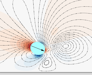

1. Introduction
The swimming of microorganisms in natural and biological environments is considerably influenced by confined boundaries within enclosed spaces (Li Reference Li2023). These boundaries guide microswimmer behaviour through surface–microorganism interaction. Bacteria are stably captured, which accumulate on walls, facilitating the formation of biofilms (Li et al. Reference Li, Bensson, Nisimova, Munger, Mahautmr, Tang and Brun2011; Dey, Saha & Chakraborty Reference Dey, Saha and Chakraborty2020). Walls also have a remarkable impact on the movement of microswimmers near boundaries. The vaginal walls of mammals guide sperms to the egg (Denissenko et al. Reference Denissenko, Kantsler, Smith and Kirkman-Brown2012), and freely swimming male and female brown algae have a probability of encountering each other near boundaries (Kinoshita et al. Reference Kinoshita, Shiba, Inaba, Fu, Nagasato and Motomura2016). Microswimmers exhibit a variety of behaviours near solid boundaries, such as various wall responses of Chlamydomonas (Li & Ardekani Reference Li and Ardekani2014), the reverse movement of sperm along walls (Miki & Clapham Reference Miki and Clapham2013), distinct motion patterns of Volvox (Drescher et al. Reference Drescher, Dunkel, Cisneros, Ganguly and Goldstein2011) and circular swimming in different directions by flagellated bacteria (Lauga et al. Reference Lauga, DiLuzio, Whitesides and Stone2006; Di Leonardo et al. Reference Di Leonardo, Dell'Arciprete, Angelani and Iebba2011). The advancement of microfluidic technology has aided the application of artificial microswimmers in areas such as laboratory devices (Bechinger et al. Reference Bechinger, Di Leonardo, Löwen, Reichhardt, Volpe and Volpe2016), cell manipulation (Bunea & Taboryski Reference Bunea and Taboryski2020) and micromotor propulsion (Poddar, Bandopadhyay & Chakraborty Reference Poddar, Bandopadhyay and Chakraborty2019; Chen et al. Reference Chen2021). Furthermore, the design of complex boundaries in microfluidic devices (protrusions and obstacles) has developed various artificial microswimmers (Simmchen et al. Reference Simmchen, Katuri, Uspal, Popescu, Tasinkevych and Sánchez2016).
The squirmer is a typical propulsion model for microswimmers (Lighthill Reference Lighthill1952; Blake Reference Blake1971a,Reference Blakeb), where self-propulsion is achieved by applying a specific tangential slip velocity on its surface. This propulsion is categorized into front-propelled pullers and rear-propelled pushers and is used to describe the movement of various representative microorganisms such as Bacillus subtilis, Chlamydomonas reinhardtii, Escherichia coli and Volvox. It is extensively used to explore the hydrodynamic properties of microswimmers, including the behaviour of squirmers in vertical pipes (Guan, Lin & Nie Reference Guan, Lin and Nie2022; Ying et al. Reference Ying, Jiang, Nie and Lin2022; Nie et al. Reference Nie, Ying, Guan, Lin and Ouyang2023), their movement in different background flow fields (More & Ardekani Reference More and Ardekani2021; Liu, Ouyang & Lin Reference Liu, Ouyang and Lin2022; Guan & Lin Reference Guan and Lin2023), swimming in non-Newtonian fluids (De Corato, Greco & Maffettone Reference De Corato, Greco and Maffettone2015; Nganguia & Pak Reference Nganguia and Pak2018; Ouyang, Lin & Ku Reference Ouyang, Lin and Ku2018) and their behaviour near walls (Kuron et al. Reference Kuron, Stärk, Holm and De Graaf2019; Chaithanya & Thampi Reference Chaithanya and Thampi2021; Ishimoto, Gaffney & Smith Reference Ishimoto, Gaffney and Smith2023). The diffusion (Ishikawa & Pedley Reference Ishikawa and Pedley2007), nutrient absorption (Magar & Pedley Reference Magar and Pedley2005) and rheological properties (Uspal et al. Reference Uspal, Popescu, Dietrich and Tasinkevych2015) of squirmers have also been thoroughly studied.
Previous studies have primarily focused on spherical or circular squirmers. However, ~80 % of bacteria and microorganisms are elongated, with an average aspect ratio of ~3. The motility of squirmers increases with their aspect ratio (Dusenbery Reference Dusenbery2009). The body shape of phytoplankton elongates as their volume increases (Gibson, Atkinson & Gordon Reference Gibson, Atkinson and Gordon2007) in organisms such as C. reinhardtii, Paramecium and E. coli. Zöttl & Stark (Reference Zöttl and Stark2013) extended the model of spherical squirmers to elongated squirmers in Poiseuille flow. They reported that the frequency of oscillation and tumbling depended on the aspect ratio although their trajectories were similar. Kyoya et al. (Reference Kyoya, Matsunaga, Imai, Omori and Ishikawa2015) studied Stokes flow around ellipsoidal squirmers, noting that the collective movement of squirmers is primarily influenced by their aspect ratio. This highlights the role of the squirmer shape in collective motion. Zantop & Stark (Reference Zantop and Stark2020) introduced the squirmer rod model and compared it with spherical squirmers to find the generation of complex fluid dynamic multipole moments by squirmer rods. Ouyang & Lin (Reference Ouyang and Lin2021) established a squirmer rod model comprising multiple spherical squirmers and studied their movement in fluid. They found that the swimming speed and the energy consumption of pullers and pushers vary with the number of spherical squirmers and their proximity. Zantop (Reference Zantop2023) investigated the collective dynamical behaviour of neutral-, puller- and pusher-type squirmer rods and reported various states ranging from disordered to clogged states. This study indicated the role of flow field types and squirmer rod density in the transition of squirmer rod movement states. Ashtari et al. (Reference Ashtari, Pourjafar-Chelikdani, Gharali and Sadeghy2022) used a no-slip condition and studied the movement of elliptical squirmers in a planar channel made of flexible membranes. They found that the aspect ratio of an elliptical squirmer has a significant impact on the movement and transport of squirmers, and demonstrated how elliptical squirmers differ from the spherical squirmers in a fluid dynamics environment. Compared with spherical squirmers, elliptical squirmers move faster at specific Reynolds numbers, providing important insights for the design of artificial microswimmers.
The above studies are based on no-slip boundary conditions on the wall. The slip phenomenon at the solid–fluid interface is a complex behaviour resulting from the interaction of various physicochemical parameters such as wettability, surface roughness, impurities and dissolved gases, which is commonly observed on hydrophobic surfaces. The slip length, defined as the hypothetical distance from the solid–fluid interface to the point where the fluid velocity extrapolates to zero, is a key metric for measuring the slip phenomenon. There have been some studies on slip boundary conditions. Choi, Westin & Breuer (Reference Choi, Westin and Breuer2003) discovered that the slip length (~30 nm) of water on hydrophobic surfaces is approximately linearly related to the shear rate. Cottin-Bizonne et al. (Reference Cottin-Bizonne, Cross, Steinberger and Charlaix2005) confirmed the existence of boundary slip and proposed that a slip length of 20 nm is consistent with theories and simulations for non-wetting smooth surfaces. Joseph & Tabeling (Reference Joseph and Tabeling2005) increased experimental precision and found that slip lengths are generally <100 nm. Huang et al. (Reference Huang, Sendner, Horinek, Netz and Bocquet2008) used molecular dynamics simulations to study the hydrodynamic slip of water on hydrophobic surfaces, finding that slip lengths ranged from nanometres to tens of nanometres, thereby resolving previous disputes regarding these measurements. In addition to nanometre-scale slip lengths, micrometre-scale slip lengths can exist under certain physical and chemical conditions. Zhu & Granick (Reference Zhu and Granick2001) pointed out that shear-induced bubble nucleation could form a gas film, which significantly increased the slip length. Tretheway & Meinhart (Reference Tretheway and Meinhart2002) discovered that applying a hydrophobic monolayer coating on microchannel surfaces produced a slip length of ~1 mm. Thus, the slip at the solid–fluid interface can be modelled as a uniform partial slip at the microscale level. Currently, wall slip conditions are widely applied in research on autonomous underwater vehicles (Guo & Hou Reference Guo and Hou2023) and in exploring the stability of liquid flow (Samanta Reference Samanta2017).
Slip boundaries do influence the swimming behaviour of microswimmers near walls. The swimming pattern of E. coli near walls forms circular trajectories, which is related to the counter-rotation of its body and flagellar bundle. Lemelle et al. (Reference Lemelle, Palierne, Chatre, Vaillant and Place2013) explained the relation between the circular motion of E. coli and slip at the solid–fluid interface, suggesting that biopolymers and surfactants controlling bacterial motility could be a novel therapeutic strategy. Hu et al. (Reference Hu, Wysocki, Winkler and Gompper2015) reported that the motion of E. coli shifted from clockwise circular trajectories to linear or counterclockwise circular trajectories with an increase in the slip length. Lopez & Lauga (Reference Lopez and Lauga2014) used far-field hydrodynamic methods to simulate the swimming of helical flagellated bacteria near walls and found that the slip boundary reoriented the cells parallel to the surface and attracted them to the surface. Their research has potential applications in the separation of individual cells. Ketzetzi et al. (Reference Ketzetzi, De Graaf, Doherty and Kraft2020) noted that the propulsion speed of microswimmers near walls was affected by the slip length of the wall. Poddar, Bandopadhyay & Chakraborty (Reference Poddar, Bandopadhyay and Chakraborty2020) further explored the mechanism affecting the swimming speed of microswimmers near walls by the slip length, demonstrating changes in the trajectories of puller- and pusher-type swimmers. Ghosh & Poddar (Reference Ghosh and Poddar2023) studied the coupling between wall slip and external flow velocity gradients, indicating that the slip length significantly affects the rheological properties of microswimmers.
However, the aforementioned studies on the motion of microswimmers near walls under slip boundary conditions have primarily focused on circular or spherical microswimmers. The geometric shape of microswimmers affects their stable swimming states in general flow fields. Hence, it can be inferred that the geometric shape of microswimmers also influences their swimming states near walls. This paper aimed to study the motion characteristics of elliptical microswimmers near walls under slip boundary conditions. (i) Elliptical microswimmer models with different aspect ratios were constructed based on circular microswimmers. (ii) The surface wettability of walls was simulated by combining modified reflection and mirror reflection conditions, thereby reflecting slip boundary conditions. (iii) The lattice Boltzmann method (LBM) was used to numerically simulate the dynamic behaviour of microswimmers near walls. Based on this foundation, the study analysed the swimming characteristics of puller- and pusher-type microswimmers near walls with different geometric configurations. It explored the impact of key factors such as the slip length, swimming Reynolds number, aspect ratio and swimming type parameters on swimming characteristics. Additionally, the study presents the dependency of microswimmer swimming modes on the initial swimming angle.
2. Numerical method
2.1. The lattice Boltzmann method (LBM)
The LBM with a single relaxation time mode (Qian, d'Humières & Lallemand Reference Qian, d'Humières and Lallemand1992) is used to simulate the swimming characteristics of microswimmers near a slip wall. The discrete lattice Boltzmann relation is shown in (2.1)
 \begin{equation}{f_i}(\boldsymbol{x} + {\boldsymbol{e}_i}\Delta t,t + \Delta t) - {f_i}(\boldsymbol{x},t) ={-} \frac{1}{\tau }[\,{f_i}(\boldsymbol{x},t) - f_i^{(0)}(\boldsymbol{x},t)],\end{equation}
where fi(x, t) is the distribution function for the microscopic velocity, ei is the ith direction, Δt is the time step of the simulation, τ is the relaxation time related to the fluid viscosity,  $f_i^{(0)}(\boldsymbol{x},t)$ is the equilibrium distribution function expressed as (2.2)
 \begin{equation}f_i^{(0)}(\boldsymbol{x},t) = {w_i}\rho \left[ {1 + \frac{{3{\boldsymbol{e}_i}\boldsymbol{\cdot }\boldsymbol{u}}}{{{c^2}}} + \frac{{9{{({\boldsymbol{e}_i}\boldsymbol{\cdot }\boldsymbol{u})}^2}}}{{2{c^4}}} - \frac{{3{\boldsymbol{u}^2}}}{{2{c^2}}}} \right],\end{equation}
where c = Δx/Δt represents the lattice speed, Δx is the lattice spacing, the speed of sound has the relation 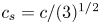 ${c_s} = c/{(3)^{1/2}}$, lattice spacing Δx and the time step Δt are fixed at 1, weights are w 0 = 4/9, w 1–4 = 1/9 and w 5–8 = 1/36, the density and velocity of the fluid are expressed as (2.3)
 \begin{equation}\rho = \sum\limits_i {{f_i}} ,\quad \rho \boldsymbol{u} = \sum\limits_i {{f_{\boldsymbol{i}}}{\boldsymbol{e}_i}} .\end{equation}
The popular D2Q9 (i.e. nine discrete velocities in two dimensions) lattice model with nine velocities is used. The discrete velocity vectors are shown in (2.4)
 \begin{equation}{\boldsymbol{e}_i} = \begin{cases} {(0,0),}&{\textrm{for}\;i = 0,}\\ {({\pm} 1,0)c,\;(0, \pm 1)c,}&{\textrm{for}\;i = 1\;\textrm{to}\;4,}\\ {({\pm} 1, \pm 1)c,}&{\textrm{for}\;i = 5\;\textrm{to}\;8.} \end{cases}\end{equation}
The macroscopic mass and momentum, expressed as (2.5) and (2.6), respectively, in the low Mach number limit, can be recovered by applying the Chapman–Enskog expansion
 \begin{gather}\frac{{\partial \rho }}{{\partial t}} + \boldsymbol{\nabla }\boldsymbol{\cdot }(\rho \boldsymbol{u}) = 0,\end{gather}
 \begin{gather}\frac{{\partial (\rho \boldsymbol{u})}}{{\partial t}} + \boldsymbol{\nabla }\boldsymbol{\cdot }(\rho \boldsymbol{uu}) ={-} \boldsymbol{\nabla }p + \rho \nu {\nabla ^2}\boldsymbol{u}.\end{gather}
2.2. Boundary conditions
The proper treatment of a moving boundary in the LBM is a critical factor in ensuring accurate simulations. Lallemand & Luo (Reference Lallemand and Luo2003) proposed an improved version of the bounce-back scheme including interpolation, which is stable, robust and easy to implement. Figure 1 shows a square and circle representing a solid and fluid node within and outside the squirmer boundary, respectively, and a triangle representing a boundary node that rebounds on the squirmer boundary. All fluid and solid nodes might change after the collision. Hence, the equilibrium distribution function from the solid node to the fluid node needs to be recalculated based on the accurate position of the boundary node (triangle presented in figure 1). The distribution function ( f 5) of the fluid node (A) was originally calculated using the solid node (B), which was inside the curved boundary. Thus, f 5 was not determined. A rebound scheme can be used to satisfy the no-slip boundary condition by setting the f 5 = f 7 condition. However, this method assumes that the boundary node (F) is exactly located at the midpoint of the line connecting two lattice nodes and is not universal. Therefore, f 5 needs to be recalculated, and a parameter q = |AF|/|AB| is introduced to determine the position of the boundary node. Finally, f 5 is recalculated based on nearby nodes (B, C and D) using an interpolation method using (2.7)
 \begin{align}{f_5}(A) = \begin{cases}
{q(1 + 2q){f_7}(B) + (1 - 4{q^2}){f_7}(A) - q(1 -
2q){f_7}(C) - 2{w_5}\rho
\dfrac{{{\boldsymbol{e}_5}\boldsymbol{\cdot
}{\boldsymbol{u}_F}}}{{c_s^2}}}&{q < \dfrac{1}{2},}\\
{\dfrac{1}{{q(2q + 1)}}{f_7}(B) + \dfrac{{2q -
1}}{q}{f_5}(C) - \dfrac{{2q - 1}}{{2q + 1}}{f_5}(D) -
\dfrac{{2{w_5}}}{{q(2q +
1)}}\dfrac{{{\boldsymbol{e}_5}\boldsymbol{\cdot
}{\boldsymbol{u}_F}}}{{c_s^2}}}&{q \ge \dfrac{1}{2}.}
\end{cases}\end{align}
The forces and torques applied to the body of microswimmers are calculated using momentum exchange methods via scanning every fluid–solid boundary link (Lallemand & Luo Reference Lallemand and Luo2003). We used the method proposed by Aidun, Lu & Ding (Reference Aidun, Lu and Ding1998) during the motion of the microswimmer involving the coverage and creation of fluid nodes to calculate these additional forces and torques (including the repulsive force in (2.11)). The total force and torque are obtained by integrating the obtained force and torque on the squirmer surface. Therefore, the motion trajectory of the microswimmer is determined by solving Newton's equations of motion based on the resultant forces and torques.
Schematic of the bounce-back scheme in the LBM.

2.3. Squirmer model
2.3.1. Circle squirmer
The squirmer model can be achieved by adding oscillatory fluctuations in the radial and tangential directions to the boundaries of particles using (2.8) (Blake Reference Blake1971a,Reference Blakeb)
 \begin{equation}{\boldsymbol{u}^s}(\boldsymbol{\theta }) = \sum\limits_{n = 0}^\infty {{A_n}\cos (n\theta )\hat{\boldsymbol{r}}} + \sum\limits_{n = 1}^\infty {{B_n}\sin (n\theta )\hat{\boldsymbol{\theta }}} .\end{equation}
Here,  $\hat{\boldsymbol{r}}$ and
 $\hat{\boldsymbol{\theta }}$ are radial and tangential unit vectors at one point on the surface of the squirmer, as shown in figure 2(a) and An and Bn are the corresponding time-dependent amplitudes, respectively. The radial component is usually ignored in problems related to the squirmer motion. Hence, a simplified squirmer model represented by a second-order truncated tangential velocity (n ≤ 2) is expressed using (2.9)
 \begin{equation}{u^s}(\theta ) = {B_1}\sin \theta + {B_2}\sin \theta \cos \theta .\end{equation}
Schematic diagram of squirmers moving to the right. (a) Circle squirmer and (b) ellipse squirmer.

The coefficient B 1 determines the self-propulsion strength of the microswimmer, thus determining its steady-state swimming velocity (Us) under Stokes flow conditions of B 1/2. The coefficient (B 2) influences the vorticity strength around the microswimmer and β = B 2/B 1 is typically introduced as a key parameter to characterize different types of microswimmers: (i) puller-type microswimmers (β > 0), such as E. coli and B. subtilis, which obtain thrust from their rear end, (ii) pusher-type microswimmers (β < 0), such as C. reinhardtii, which obtain thrust from their front end (Koch & Subramanian Reference Koch and Subramanian2011) and (iii) neutral-type microswimmers (β = 0), which are associated with vortex-free symmetric flows (Fadda, Molina & Yamamoto Reference Fadda, Molina and Yamamoto2020), such as Volvox.
2.3.2. Ellipse squirmer
Inspired by the work of Zantop & Stark (Reference Zantop and Stark2020) who took a squirmer rod as a combination of several circular squirmers with equal diameters, in our model of elliptical squirmer, the velocity at each point (e.g. E in figure 2b) on the surface of elliptical squirmer is equal to the velocity at the point on the surface of circular squirmer that is tangent to that point, as shown in figure 2(b).
In the computation, we choose enough computed nodes (e.g. E in figure 2b) on the surface of elliptical squirmer and sufficiently small spacing between adjacent squirmers to ensure high accuracy and continuity of tangential velocity at the computed nodes on the surface of the elliptical squirmer.
To demonstrate the effectiveness of the above model, we compare the swimming speed computed using the model of elliptical squirmer with that given by analytical solution,  $2Us/\{ {B_1}\ast [1 + ({C_{ab}} - 1)/({C_{ab}} + 1)]\}$, as shown in figure 6(b), obtained from the conformal theorem (mapping a circle to a ellipse) (Liu et al. Reference Liu, Ouyang and Lin2022). The two results are consistent.
For guaranteeing the continuity of surface velocities on the elliptical squirmer, before officially starting the computation, we conducted a trial run and choose enough points on the surface of the elliptical squirmer for computation. Besides, the specific implementation method for the elliptical squirmer is as follows: according to the method outlined in § 2.3, it is possible to determine the boundary nodes and the normal vectors of the elliptical squirmer, as shown at point E and vector n in figure 1. Then, an inscribed circle, circle 1, which shares the same node E and normal vector n, can be determined, and the tangential velocity at point E on circle 1 is mapped onto the ellipse. This process is repeated until the tangential velocities at all boundary points on the ellipse are derived from the circle.
2.4. Repulsive force model
Collisions might occur when swimmers approach a wall. Thus, we adopted the repulsive force model proposed by Glowinski et al. (Reference Glowinski, Pan, Hesla, Joseph and Periaux2001) to resolve collision issues. This model has been widely applied in many studies (Ouyang et al. Reference Ouyang, Lin and Ku2018; Ying et al. Reference Ying, Jiang, Nie and Lin2022; Nie et al. Reference Nie, Ying, Guan, Lin and Ouyang2023) and has been proven to be effective and reliable for simulating interactions between swimmers and the wall. In this model, the collision between swimmer and the wall is assumed to be smooth, i.e. precaution will be taken to avoid overlapping of the regions occupied by the swimmer and wall when a swimmer collides with the wall surface. To achieve this goal, a short-range repulsive force is given
 \begin{equation}F_{ij}^w = \begin{cases}
0&{\textrm{if}\;{d^{\prime}_{ij}} > {R_i} + {R_j} + \xi
}\\ {\dfrac{{{c_{ij}}}}{{{\varepsilon_w}}}{{\left(
{\dfrac{{{R_i} + {R_j} + \xi - {d^{\prime}_{ij}}}}{\xi }}
\right)}^2}\dfrac{{({\boldsymbol{G}_i} -
{{\boldsymbol{G^{\prime}}}_j})}}{{{d^{\prime}_{ij}}}}}&{\textrm{if}\;{d^{\prime}_{ij}}
\le {R_i} + {R_j} + \xi }
\end{cases}.\end{equation}
Here, Ri represents the radius of a squirmer with the centroid located at Gi, and  ${\boldsymbol{G^{\prime}}_j}$ is the centroid position of a hypothetical squirmer located inside the wall, as shown in figure 3. Also,
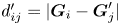 ${d^{\prime}_{ij}} = |{\boldsymbol{G}_i} - {\boldsymbol{G}^{\prime}_j}|$ is the distance between two centroids, ξ is a cutoff distance below which the repulsive force would come into effect, which is set to 1.5 Δx. The reason for setting 1.5Δx as the cutoff distance instead of other values is that it can achieve the required calculation accuracy (referring to 3.4) while avoiding the need for too much calculation time. The parameter εw is a given positive stiffness coefficient set to 10−3 and cij is a force scaling factor and is defined as the difference between the gravitational and buoyancy forces of the squirmer in the simulations.
Schematic diagram of the repulsive force model. (a) Circle and (b) ellipse.

The original repulsive force in (2.10) was designed for circular particles. Therefore, we modified this formula to accommodate collisions involving elliptical particles. The modified expression of the repulsive force is given as (2.11). The label Ns presented in figure 3(b) represents the point on the elliptical particle closest to the wall, while Nw (figure 3b) is the position on the wall corresponding to that point. Thus, |Ns−Nw| represents the minimum distance from the elliptical particle to the wall. Unlike circular particles, the repulsive force from the wall to the elliptical particle might not necessarily point toward its centroid. This repulsive force generates a torque on the elliptical particle. Hence, this torque must be considered in calculations as expressed in (2.11)
 \begin{equation}F_{ij}^{we} = \begin{cases} 0&{\textrm{if}\;|{\boldsymbol{N}_s} - {\boldsymbol{N}_w}|> \xi }\\ {\dfrac{{{c_{ij}}}}{{{\varepsilon_w}}}{{\left( {\dfrac{{|{\boldsymbol{N}_s} - {\boldsymbol{N}_w}|- \xi }}{\xi }} \right)}^2}\dfrac{{({\boldsymbol{N}_s} - {\boldsymbol{N}_w})}}{{|{\boldsymbol{N}_s} - {\boldsymbol{N}_w}|}}}&{\textrm{if}\;|{\boldsymbol{N}_s} - {\boldsymbol{N}_w}|\le \xi } \end{cases}.\end{equation}
2.5. Slip boundary conditions
For the slip boundary conditions of the wall we combined the methods of reflection and mirror reflection conditions (Wang et al. Reference Wang, Chai, Hou, Chen and Xu2018). Figure 4 illustrates the application of this method using the D2Q9 model; j presented in figure 4 represents the jth layer of grids and s (figure 4) is the force driving the fluid flow along the x-axis with the y-axis in the vertical direction. The distribution functions f 0, f 1, f 3, f 4, f 7 and f 8 for nodes can be determined during the flow process, but f 2, f 5 and f 6 remain unknown. These unknown distribution functions are defined as (2.12)–(2.14) (Succi Reference Succi2002)
 \begin{gather}{f_2} = {f_4},\end{gather}
 \begin{gather}{f_5} = {r_1}\,{f_7} + (1 - {r_1}){f_8} + 2{r_1}\rho {\omega _i} \cdot {u_w}/2c_s^2,\end{gather}
 \begin{gather}{f_6} = {r_1}\,{f_8} + (1 - {r_1}){f_7} + 2{r_1}\rho {\omega _i} \cdot {u_w}/2c_s^2,\end{gather}
where uw represents the velocity of the wall and r 1 is the adjustment coefficient . The value of r 1 is calculated using (Wang et al. Reference Wang, Chai, Hou, Chen and Xu2018)
 \begin{equation}{r_1} = \frac{1}{{1 + \dfrac{{{l_s}}}{\tau }}},\end{equation}
where ls is the slip length, τ is the is the relaxation time related to the fluid viscosity and r 1 is a crucial parameter linking the slip length ls with the boundary slip effect. Using (2.15), ls in the code can be adjusted to match the experimental result.
Boundary grid for the slip boundary conditions using the D2Q9 model.

3. Flow parameters and validation of method
3.1. Flow field parameters
Figure 5 presents a schematic of a microswimmer approaching a wall with slip boundary conditions. The numerical simulations have the following fluid domains: length (L), width (H), density (ρ) and viscosity (ν). The density of the microswimmer is denoted as ρs. The diameter of the circular microswimmer is d, while the major and minor axes of the elliptical microswimmer are 2a and 2b (2b = d), respectively, with an aspect ratio Cab = a/b. The angle between the swimming direction of the microswimmer and the x-axis is represented by θ. In order to simulate an infinitely long area in the x-direction, a method of moving computational domain is used, i.e. both the flow and the position of the microswimmer shift to the left by one lattice spacing when the microswimmer moves beyond a distance of X 0 + Δx from its initial position. Using this method can ensure that microswimmers do not escape the computational domain, while significantly reducing the required number of computational grids and improving resolution. A boundary condition of fully developed non-equilibrium extrapolation is applied to the upper boundary. Using this boundary condition can ensure that the upper boundary does not affect the flow near the wall surface.
Schematic diagram of squirmer towards a slip boundary.

The swimming Reynolds number (Res) is introduced to describe the self-propulsion strength of the microswimmer, as defined in (2.15), where Us = B 1/2. Variations in the self-propulsion strength of the microswimmer can be achieved by changing the value of Res. Unless specifically stated, the values of some parameters in numerical simulations are as mentioned: L = 12d, H = 8d, ρ = 1, ρs = 1, Res ranges from 0.01 to 1 and d = 40. The initial position of the microswimmer is set to X 0 = 0.5L and Y 0 = h = 0.4H with an initial swimming angle of θ 0 = −0.1 ${\rm \pi}$
 \begin{equation}R{e_s} = \frac{{{U_s}d}}{\nu },\end{equation}
3.2. Squirmer model validation
The squirmer model presented in § 2.3 (2.9) was validated via numerical simulations of a single squirmer freely swimming in a 25d × 25d square region with all the boundaries of the region set as periodic boundary conditions. The simulated squirmers were both circular and elliptical with an aspect ratio of Cab = 2.0. Their swimming speeds were normalized using Us/(B 1/2) for the circular squirmer and Us/[(B 1/2) × (1 + (Cab−1)/(Cab + 1))] for the elliptical squirmer. Figure 6 shows the results of the swimming speeds of neutral (β = 0), puller (β = 5) and pusher (β = −5) squirmers tending toward their theoretical speeds. It is evident that both circular and elliptical swimming speeds eventually converge to the theoretical speeds. This indicates that the circular and elliptical squirmer models used in this paper are credible. Terminal swimming velocity in figure 6 is based on Res = 0.01 rather than a larger value, the reason is that we want to confirm whether the terminal swimming velocity of microswimmers reaches the theoretical value B 1/2 under the Stokes flow condition (extremely low Reynolds numbers) when using the squirmer model. Due to the fact that validation is carried out under specific conditions such as Stokes flow, choosing Res = 0.01 is typical.
Terminal swimming velocity for a freely swimming squirmer (Res = 0.01 and d = 40); (a) Cab = 1.0 and (b) Cab = 2.0.

We also performed a grid independence verification. The results of the swimming speeds at different mesh densities are shown in figure 7, where the diameter d of the squirmer is 5, 10, 20, 40 and 80. When d ≥ 20, the stable swimming speed of the squirmer reaches the theoretical speed, and the speed curve is smooth and stable. Considering factors such as accuracy and computational time, we chose d = 40 in the simulation.
Swimming speed for a freely swimming squirmer under different mesh divisions.

3.3. Slip boundary validation
This section validates the slip boundary conditions. Figure 8(a) shows the two-dimensional shear flow field features of a top plate moving at a uniform speed of U 0 = 0.04, while the bottom plate remains stationary under slip boundary conditions. Periodic boundary conditions are applied at the inlet and outlet; Nx and Ny represent the number of grids along the X and Y directions, respectively. Figure 8(b) shows the computational results for different grid numbers (Nx × Ny) under slip boundary conditions. The results from different grid numbers are almost identical, providing a basis for the selection of grid numbers in the simulations. Additionally, this demonstrates that the calculated ls closely matches the theoretical result (ls 0).
Validation of slip boundary conditions. (a) Calculation area and (b) grid independence verification.

3.4. Cutoff distance validation
In § 2.4, we mentioned the cutoff distance, ξ. To determine ξ, we conducted more detailed numerical simulations for ξ = 1.2Δx, 1.5Δx, 2.0Δx and 2.5Δx, and the trajectories of the squirmer at different ξ are shown in figure 9, where the impact of ξ on the trajectories of the squirmer is very small, so we chose ξ = 1.5Δx because it can achieve the required calculation accuracy while avoiding the need for too much calculation time.
Trajectories of the squirmer at different cutoff distances ξ(Res = 0.08, β = 3, ls = 3).

4. Results and discussion
4.1. Movement of squirmers with different Cab values
Figure 10 displays the instantaneous streamlines around squirmers with different aspect ratios. The puller (β = 1) propels by pulling the fluid from the front and experiences restricted movement near the wall, thereby affecting the structure of streamlines. The pusher (β = −1) propels by pushing the fluid from the rear and has a different streamline distribution near the wall than that of the puller. Thus, different propulsion methods result in distinct streamlined structures around pullers and pushers. The distribution of streamlines around neutral (β = 0) squirmers resembles passive particles. A comparison of figures 10(a)–10(c) shows that the surrounding streamlines and velocity distributions vary for squirmers with different Cab values. A recirculation area at the head of the puller increases with increasing aspect ratio Cab when β = 1. Conversely, the recirculation area at the tail of the pusher gradually decreases when β = −1. This reflects the differences in the self-propulsion methods of squirmers and the degree of interaction between squirmers with different Cab values and the wall.
Instantaneous streamlines and the velocity field around a squirmer (Res = 0.08, θ 0 = −0.1 ${\rm \pi}$, h = 0.2H); (a) Cab = 0.8, (b) Cab = 1.0 and (c) Cab = 1.2.

4.2. The interaction between a puller and the wall
Figure 11 presents the phase diagram of the final states of a puller, revealing four distinct motion states: escape, oscillation, sliding along the wall and wall lock-up. The escape state occurs when the self-propulsion strength (β) is relatively low. The puller cannot escape from the wall once β exceeds a certain critical value and is found in one of the other three states. The puller exhibits a transitional change near the wall as the β value changes, oscillating to sliding along the wall and finally locking up. Figure 12 shows the trajectories of the puller in these four states, illustrating that, apart from escape, the other three states occur near the wall.
Phase diagram of the final states of a puller with different Cab values, solid circle: wall escape, solid square: oscillation near the wall, hollow square: sliding along the wall and solid triangle: wall lock-up (the region from  ${\rm \pi}$/2 to 7
 ${\rm \pi}$/6: Res = 0.08, the region from 7
 ${\rm \pi}$/6 to 11
 ${\rm \pi}$/6: Res = 0.8, the region from 11
 ${\rm \pi}$/6 to
 ${\rm \pi}$/2: Res = 0.4, the radii of the circle, from innermost to outermost, represent ls values of 0, 0.1, 0.5, 1, 5, 10, respectively); (a) Cab = 0.8, (b) Cab = 1.0, (c) Cab = 1.2 and (d) Cab = 2.0.

Movement trajectories of a puller in the four different states.

4.2.1. Wall-escape state of the puller
Figure 13(a) shows the variation of the horizontal velocity (Vx) of a puller during swimming as a function of the relative distance h/H from the wall under different ls. The puller initially moves toward the wall from a distance of 0.4H, moves away from the wall under its influence and returns to a position of 0.4H away from the wall. The value of Vx gradually increases during the approach toward the wall; Vx first decreases and then increases on moving toward and away from the wall, respectively. The trend in the change of Vx remains the same as ls increases, but the puller moves close to the wall (small h/H values). There is a significant velocity gradient in the narrow gap between the puller and the wall when the puller approaches the wall. A large ls weakens this velocity gradient. This conclusion is confirmed by the instantaneous streamline and vorticity diagrams, as shown in figure 14. Vorticity between the puller and wall with a ls of 10 is smaller than that without a slip length (ls = 0). In addition, horizontal velocity of the puller increases with increasing aspect ratio Cab. The reason is that, on the one hand, the shape of the microswimmer transitions from circular to elliptical as Cab increases, becoming more streamlined and thereby reducing the flow resistance and allowing for an increase in Vx. On the other hand, the tangential velocity and its related Vx on the surface of an elliptical squirmer increases as Cab increases. At ls = 10, there's a noticeably distinct behaviour around h/H = 0.1 compared with other ls values. On the one hand, the closer to the wall, the greater the effect of ls, h/H = 0.1 is closest to the wall compared with other positions, so there is a noticeably distinct behaviour around h/H = 0.1. On the other hand, the larger the value of ls, the greater the effect of reducing the velocity gradient between the wall and the microswimmer, which allows the microswimmer to swim closer to the wall at ls = 10, thereby causing changes in speed and swimming angle and triggering different motion behaviours.
Variation in the horizontal velocity, torque experienced and swimming angle of a puller relative to its distance from the wall under different ls values (θ 0 = −0.1 ${\rm \pi}$, Res = 0.08 and β = 1). (a) Horizontal velocity of pullers, (b) torque experienced of pullers and (c) swimming angle of pullers.

Instantaneous streamline and vorticity diagrams around a puller at different ls values (θ 0 = −0.1 ${\rm \pi}$, Res = 0.08, β = 1, Cab = 0.8, h/H = 0.2); (a) ls = 0 and (b) ls = 10.

Figure 13(b) shows that the torque experienced by the puller decreases with an increase in ls at the same relative distance of h = 0.2H from the wall, inducing the puller to swim close to the wall when ls values are high. This explains the variation in the swimming angle of the puller at different ls values, as shown in figure 13(c). The larger the aspect ratio Cab, the greater the torque variation during the interaction between the puller and the wall.
The escape state of a puller occurs when the values of β and Res are relatively low, as previously mentioned and illustrated in figure 11. Ishimoto & Gaffney (Reference Ishimoto and Gaffney2013) reported that the puller would not generate a hydrodynamic rotation toward the wall when the value of β was not very high. However, the puller would produce additional rotation and form a movement pattern near the wall when β exceeds a certain critical value. The phase diagram presented in figure 15 elaborates on the influence of the ls and Cab values of the puller on its movement patterns to investigate the mechanism behind this phenomenon (Res = 0.08 and β ≤ 2). The grey area (figure 15) represents the escape state of the puller, while the yellow area (figure 15) indicates the state where the puller is captured by the wall. The corresponding initial angle is θ 0 = −0.1 ${\rm \pi}$, as the attraction of the wall on the puller can be neglected for θ 0 > 0 (Li & Ardekani Reference Li and Ardekani2014). Figure 15 shows that the puller is captured (yellow area) only when both β and ls are relatively large for the three values of Cab because an increased ls changes the characteristics of the interaction between the puller and wall. The puller is in the escape state (grey area, figure 15) below the critical value (βc) (β < βc). The value of βc increases with the increase of Cab, suggesting that the pullers with a high Cab have a high probability of escaping from the wall at Res = 0.08 and β ≤ 2. The reason is that the swimming speed of the microswimmer increases with increasing Cab, while the higher speed gives the microswimmer a greater repulsive force after colliding with the wall, which makes it easier for the microswimmer to escape from the wall.
Phase diagram of the final states of a puller. Grey area: escape state and yellow area: wall capture state (Res = 0.08); (a) Cab = 0.8, (b) Cab = 1.0 and (c) Cab = 1.2.

4.2.2. Periodic oscillation state of the wall capture of pullers
An increase of ls value would prompt the puller to change from an escape state to a periodic oscillating wall capture state. Figure 16(a) shows the puller transition from an escape state to an oscillating state when ls exceeds a certain critical value. Figure 16(b) shows the swimming angle (θ) of the puller deflecting upward as it approaches and collides with the wall, generating an upward velocity component that drives the puller away from the wall. The deflection of θ is the result of the combined effect of factors such as self-propulsion, wall effect, repulsive force and the pressure distribution around the puller. As time progresses and the distance between the puller and wall increases, the influence of the wall gradually diminishes. The propulsive force driving the puller toward the wall is dominant, reversing θ and the direction of the puller to propel toward the wall again. The limit cycle in figure 16(b) is a special pattern of system behaviour, in which the state of the system (such as the position and angle of the microswimmer) periodically returns to its initial state over time. In the pattern diagram, it appears as a closed loop.
Transition of puller's swimming state at different ls (Cab = 1.0, Res = 0.08 and β = 1.6). (a) Trajectory and (b) angle height.

Figure 16(a) shows that the periodic oscillatory trajectory of the puller changes with an increase of ls. The trajectory of the puller undergoes small-scale and large-amplitude oscillations before being captured by the wall, reaching its maximum amplitude during the first departure from the wall. This maximum amplitude decreases as ls increases. Figure 17 demonstrates that the amplitude (ha) and frequency ( f) of the periodic oscillation of the puller change with variations in ls. We can see that, as ls increases, ha decreases and f increases. The reason is that there is a velocity gradient in the narrow gap between the puller and the wall when the puller approaches the wall, the larger the value of ls, the greater the effect of reducing the velocity gradient, which allows the puller to swim closer to the wall, thereby causing the oscillation of puller to be suppressed by the wall, i.e. decreased in amplitude ha. While ha decreases, the oscillation frequency f increases. The curve fitting presented in figure 17 indicates that, when ls increases logarithmically, the changes in ha and f are not in a straight line. From a mathematical perspective, this fitting relationship can be used to relatively easily calculate ha and f when ls is known.
Periodic oscillation state of wall capture for a puller at different ls (Cab = 1.0, Res = 0.4, β = 1).

Figure 18(a) shows the change in the periodic oscillatory trajectory of the puller with its Cab. The trajectory of the puller undergoes small-scale large-amplitude oscillations with the maximum amplitude increasing as Cab increases. The maximum amplitude exceeds the initial distance between the puller and wall at Cab = 1.2. The range of large-amplitude oscillations also significantly increases as Cab increases, which is opposite to the case of increasing ls, as shown in figure 16(a). In figure 18(b), we display the response of the ha value and frequency f of the puller as Cab changes from 0.8 to 1.2. The results show that, as Cab increases, the growth of ha is quite noticeable, particularly when Cab increases from 0.8 to 1.0, where ha accelerates quickly, then the rate of increase slows down towards Cab = 1.2. This indicates that the ha of the puller is sensitive to increases in Cab. In contrast, the changes in f are relatively stable, overall demonstrating insensitivity to changes in Cab.
Periodic oscillation state of wall capture for a puller at different Cab (Res = 0.4, β = 1, ls = 0.1). (a) Trajectory and (b) ha, f vs. Cab.

4.2.3. Stable sliding state of pullers
The swimming state of the puller changes from a periodic oscillatory wall capture state to a stable wall-sliding state as ls increases, where the puller slides parallel to the wall in a fixed configuration. Figure 19(a) shows a periodic oscillation state of the puller when ls ≤ 0.3, forming a limit cycle in the phase diagram. Oscillation dampens and eventually becomes a stationary point in the phase diagram when ls surpasses a critical value. This transition can be attributed to the unique pressure distribution in the flow around the puller. Figure 19(a) illustrates a large θ value of the puller as it approaches the wall with an increase of ls, enhancing the interaction between the low-pressure area near the head of the puller and wall. The ability of the puller to reorient diminishes with the strengthening of this interaction, causing the swimming mode to change from periodic oscillation to wall sliding.
Swimming angle, streamline and pressure distribution of the flow field around a puller when Cab = 0.8(Res = 0.08 and β = 5). (a) Swimming angle and (b) streamline motion and pressure distribution (ls = 0.5).

Significant differences in the swimming behaviour of pullers with different Cab values in the steady sliding state are observed. Figure 20(a) displays the steady sliding state of a puller when Cab = 1.0. A series of magnified repeated line segments show clear periodicity. The differences in the swimming behaviour of pullers with varying Cab values are presented in figures 19(b) and 20(b), where the streamline and pressure distributions in the steady sliding state are shown for Cab = 0.8 and Cab = 1.0, respectively. Although the movement modes of the pullers are similar in both cases (sliding is parallel to the wall at a fixed height), their configurations are different. The puller is inclined toward the wall with asymmetric pressure and streamline distributions when Cab = 0.8, allowing a stable slide near the wall. Alternately, the pressure and streamline distributions are almost symmetric with slight asymmetry causing the puller to slide slowly near the wall when Cab = 1.0.
Swimming angle, streamline flow and pressure distribution of the flow field around a puller when Cab = 1.0 (Res = 0.08 and β = 5). (a) Swimming angle and (b) streamline and pressure distribution (ls = 0.8).

Figure 21(a) shows the trajectory of a puller in the steady sliding state when Cab = 0.8. Thus, the puller gradually moves closer to the wall as ls increases. The inset in figure 21(a) indicates that the tilt angle of the puller enlarges with increasing ls with a decreasing speed. Figure 21(b) shows that the oscillation amplitude of the tilt angle of the puller decreases as ls increases when Cab = 1.0. This is reflected in both the maximum and minimum values of the swimming angle of the puller decreasing and eventually stabilizing within a range of ~−90° (perpendicular to the lower wall) ± 1.5°, with an amplitude of ~3°. Thus, ls significantly influences the swimming angle of the puller near the wall, affecting its swimming speed and subsequent movement patterns.
State of wall steady sliding of pullers with different Cab (Res = 0.4 and β = 5.0); (a) Cab = 0.8 and (b) Cab = 1.0.

4.2.4. Wall lock-up state of pullers
The parameter Cab plays a crucial role in the formation of the wall lock-up state for pullers. Figure 11 shows that the wall lock-up state occupies only a small area when Cab = 0.8 and 1.0, this state covers more than two thirds of the area when Cab = 1.2. The mode almost spans the entire area when Cab = 2.0. Ishimoto (Reference Ishimoto2017) indicated that the asymmetry of the geometric shape of the puller causes an additional torque owing to spatial obstruction interactions as Cab increases. In this study, a large Cab indicates a high torque of the puller upon collision with the wall, as shown in figure 13(b). This increased torque rapidly changes the swimming angle of the puller. The low-pressure area between the puller and the wall intensifies when |θ| exceeds a certain critical value, leading to the capture of the puller by the wall. Consequently, the puller loses its swimming speed in the X-direction and becomes firmly locked at a specific location on the wall (figure 22a). Moreover, increasing ls brings the puller close to the wall. The closer the puller is to the wall, the greater the torque generated by the interaction with the wall, causing effects similar to increasing Cab. Figure 22(b) shows that the maximum torque induced by the collision of the puller with the wall increases with the increase of ls. This further confirms that ls affects the swimming mode of the puller, especially when the torque is generated due to the interaction with the wall.
Characteristics of the wall lock-up state for a puller (Cab = 1.2, Res = 0.4 and β = 5). (a) Streamline and pressure distribution (ls = 5.0) and (b) maximum torque.

4.2.5. Impact of the initial swimming angle of the pullers
This section examines the final swimming state of the puller at different initial swimming angles (θ 0). Figure 23 presents the phase diagrams of the final state of the puller for four initial swimming angle (θ 0) values, illustrating how Res, β and ls jointly affect the final state. The puller exhibits relatively uniform swimming states at different parameter settings. When β is large (β ≥ 3), the impact of θ 0 on the final state of the puller is the minimum. The puller primarily exhibits wall oscillation and wall-sliding states when Cab = 0.8 and 1.0, whereas the puller is predominantly in the wall lock-up state when Cab = 1.2, 1.5 and 2.0. The final state of the puller can shift from a wall-escape state to the wall lock-up state as θ 0 increases for small β values (β < 3). Particularly, pullers with a high Cab and small β tend to escape from the wall at small θ 0 values, indicating that pullers are more likely to detach from the wall at small θ 0.
Phase diagrams of the final state of the puller at different θ 0 values at Res = 0.08. Solid circles: wall escape, solid squares: oscillation near the wall, hollow squares: sliding along the wall and solid triangles: wall lock-up (the region from  ${\rm \pi}$/10 to
 ${\rm \pi}$/2: Cab = 1.0, the region from
 ${\rm \pi}$/2 to 9
 ${\rm \pi}$/10: Cab = 0.8, the region from 9
 ${\rm \pi}$/10 to 13
 ${\rm \pi}$/10: Cab = 2.0, the region from 13
 ${\rm \pi}$/10 to 17
 ${\rm \pi}$/10: Cab = 1.5, the region from 17
 ${\rm \pi}$/10 to
 ${\rm \pi}$/10: Cab = 1.2, the radii of the circle, from innermost to outermost, represent ls values of 0, 0.1, 0.5, 1, 5, 10, respectively); (a) θ 0 = −0.05
 ${\rm \pi}$, (b) θ 0 = −0.1
 ${\rm \pi}$, (c) θ 0 = −0.2
 ${\rm \pi}$ and (d) θ 0 = −0.3
 ${\rm \pi}$.

4.3. Interaction between pushers and the walls
The swimming behaviour of pushers also exhibits characteristics of wall capture and wall-escape states. Unlike pullers, pushers show a tendency to escape from the wall even at a high swimming Res, and the likelihood of wall escape increases with the increase in Res. However, increasing ls induces pushers to transform from a state of wall escape to that of wall capture when Res and β are the same. Figure 24 illustrates that pushers primarily exhibit three types of movement states: wall escape, oscillation and steady sliding states. Pushers do not exhibit the wall lock-up state observed in pullers, which is related to the differences in pressure and streamline distribution around the pusher and puller in the flow field. Figures 27 and 28 will further illustrate this.
Phase diagram of the final states of a pusher with different Cab (solid circle: wall escape; solid square: oscillation near the wall; hollow square: sliding along the wall); (a) Cab = 0.8, (b) Cab = 1.0, (c) Cab = 1.2 and (d) Cab = 2.0.

4.3.1. Wall-escape state of pushers
Figure 25(a) shows that the Vx value of the pusher gradually increases as it approaches the wall; Vx increases with Cab, similar to the situation of the puller depicted in figure 13(a). However, Vx first increases and then decreases when the pusher approaches the wall and begins to escape, which is opposite to the puller. This difference is attributed to the distinct torque experienced by the microswimmer near the wall and the swimming angle that determines whether it can escape, and this can be explained through the surrounding pressure distribution and streamline structure. Pullers first experience a negative torque when they approach the wall because the head of a puller is typically in a low-pressure state, thus the head is attracted by the wall, causing the swimming direction to gradually turn towards the wall. The phenomenon can be found in figure 13(c), where the swimming angle of the puller decreases initially. In contrast to pullers, pushers first experience a positive torque as they approach the wall. As shown in figure 25(c), the swimming angle of the pusher initially increases because the high-pressure region is located at the head and tail of the pusher, which leads to a tendency for the head to move away from the wall. In addition, the horizontal velocity of the pusher increases with increasing aspect ratio Cab. Figure 25(b) shows that the negative torque the pusher experiences while swimming is significantly higher than the positive torque, a contrast to the situation of the puller shown in figure 13(b). The larger the aspect ratio Cab, the greater the torque variation during the interaction between the pusher and the wall. Furthermore, the trend in the change of the swimming angle of the pusher shown in figure 25(c) also differs from that of the puller (figure 13c).
Variation in horizontal velocity, torque experienced and swimming angle of a pusher relative to its distance from the wall under different ls (θ 0 = −0.1 ${\rm \pi}$, Res = 0.08, and β = −1). (a) Horizontal velocity of pushers, (b) torque experienced by pushers and (c) swimming angle of pushers.

The different physical mechanisms during the swimming of pullers and pushers are shown in figure 26, which identifies four representative points in the process of approaching and escaping the wall for pullers and pushers. Figures 27 and 28 display the streamline and pressure distribution around the puller and pusher, respectively, at these four points. It can be observed that two recirculation zones appear around the head of the puller during the initial stage of approach to the wall with high pressure on the sides and low pressure around the head and tail of the puller (figure 27a). This unique pressure distribution causes the low-pressure area at the puller's head to be easily captured by the wall, resulting in what is called a ‘wall-locking state’. In contrast, the pressure and streamline distribution around pushers is the exact opposite of pullers (figure 28a). The pressure features around pushers are high pressure at the head and tail and low pressure at the sides, a distribution that does not favour the formation of a stable captured state near the wall. Therefore, pushers do not exhibit the wall-locking state observed in pullers. The presence of a recirculation zone on the side close to the wall disrupts the force balance on either side of pullers and pushers. Thus, the θ value of the front-driven pullers tends to tilt toward the wall, while the rear-driven θ of the pusher deviates away from the wall. The influence of the wall on the swimming intensifies as the puller and pusher approach the wall, enhancing the tendency of the θ value of the pusher to deviate away from the wall and altering the direction of the θ value of the puller toward the wall. When the puller and pusher begin to move away from the wall, the influence of the wall on their swimming diminishes, allowing them to leave the wall at a fixed θ (figures 27d and 28d). Additionally, the pusher requires a large swimming angle |θ| to escape from the wall owing to the presence of a low-pressure area between the side of the pusher and wall (figure 28c).
Four key points for pullers and pushers in the wall-escape state (points 1 and 4: h/H = 0.3, point 2: maximum T, point 3: minimum T) (Cab = 1.0, Res = 0.08, β = 1.0, and ls = 5.0). (a) Puller and (b) pusher.

Distribution of streamlines and pressure around the puller at four key points. (a) Point 1, (b) point 2, (c) point 3 and (d) point 4.

Distribution of streamlines and pressure around the pusher at four key points. (a) Point 1, (b) point 2, (c) point 3 and (d) point 4.

The θ value of the pusher continuously increases as it approaches the wall owing to the difference in propulsion methods between pullers and pushers, ensuring an angle of the pusher to move away from the wall near it. Figure 28(c) marks the forces on the pusher, revealing a balance between the high and low pressure on the tail and side, respectively. However, the angle at which the pusher moves away from the wall facilitates its escape from the influence of the wall. The phase diagram presented in figure 24 suggests that pushers have the probability of being in a wall-escape mode; ls significantly influences the θ of the pusher as it approaches the wall.
Figure 29 illustrates the variation of the swimming angle θ for pushers with different Cab as a function of ls. The value of θ decreases with a decrease of ls, and the rate of decrease of θ diminishes with increasing Cab. This behaviour occurs because an increase in ls weakens the velocity gradient in the narrow gap between the pusher and wall by bringing the pusher closer to the wall and altering interactions between the pusher and wall.
The variation of the θ of the pusher with ls for different Cab (h/H = 0.12); (a) Res = 0.08 and β = −1, (b) Res = 0.4 and β = −3 and (c) critical ls.

The changing ls changes the swimming states of the pusher when |β| is large (β = |3|). Figure 29(b) shows that a pusher with a Cab of 0.8 has a stable sliding state along the wall and θ decreases as ls increases. Alternately, the θ value of pushers decreases to a certain threshold value with Cab values of 1.0 and 1.2, owing to the increase of ls; the pusher is captured by the wall and begins to oscillate near the wall. With further decrease in θ, the oscillatory motion of the pusher eventually transforms into a stable sliding state. The critical ls value at which the pusher is captured by the wall is dependent on Cab during this process; as shown in figure 29(c), the critical value of ls gradually decreases as Cab increases.
4.3.2. Periodic oscillation state during the wall capture of the pusher
Figure 30 shows the distance from the wall and θ of pushers and pullers in the state of periodic oscillation. There are differences between the pusher and puller. The initial direction of the movement of the pusher is away from the wall, while that of the puller is toward the wall. The distance of the pusher from the wall and the amplitude of its directional oscillation are more than those of the puller with the same parameters. This indicates that the dynamic behaviour of pushers and pullers in their interaction with the wall is different, especially in terms of adjusting their swimming direction to cope with the constraints of the wall.
Changes in the distance from the wall and the swimming angle of microswimmers over time in the state of periodic oscillation (Cab = 1.0, Res = 0.08, and ls = 1.0). (a) Pusher (β = −3) and (b) puller (β = 3).

The ha and f values of the trajectories of pushers and pullers with changing ls in the periodic oscillation state are shown in figure 31. We can see that, as ls increases, ha decreases and f increases. Under the same parameters, the ha value of pushers is higher than that of pullers. A large ha allows a wide range of periodic oscillation states. The slip boundary conditions on the wall significantly impact the swimming states of microswimmers, and the extent of this impact varies between different propulsion types.
Variation of trajectory amplitude (ha) and frequency ( f) with slip length (ls) in the oscillatory state of microswimmers (Cab = 1.0 and Res = 0.08). (a) Pusher (β = −3) and (b) puller (β = 3).

Figure 32 presents the swimming behaviour of pushers with three different Cab values near the wall, revealing that all pushers exhibit an oscillatory state. However, significant differences are observed in the oscillation characteristics between the pushers with varying Cab values. The oscillation amplitude of a pusher with Cab = 0.9 (figure 32a) remains constant with an initial maximum amplitude (hima) of 31.09. Alternately, the oscillation amplitudes of the pushers with Cab = 1.0 (figure 32b) and Cab = 1.2 (figure 32c) gradually decay with hima values of 30.14 and 22.24, respectively. A comparison the f of pushers with three different Cab values shows that f is inversely proportional to Cab. The trajectory of the pusher with Cab = 1.2 reaches a stable oscillation state in the shortest time, indicating that the Cab value of microswimmers significantly affects their oscillation amplitude and frequency near walls, with a more pronounced effect in pushers.
Periodic oscillations of pushers with different Cab (Res = 0.08, β = −3, and ls = 0.1); (a) Cab = 0.9, (b) Cab = 1.0 and (c) Cab = 1.2.

4.3.3. Stable sliding state of pushers
Figure 33 presents the streamlines and pressure distribution of pushers sliding along the wall with three Cab values. Pushers are captured by the wall owing to the low-pressure areas between them and the wall, inducing their sliding movement along it. The hydrodynamic impact on the flow field varies with the Cab value of pushers, resulting in distinct flow line and pressure distributions. The arrows inside the pushers (figure 33) indicate their direction of motion, showing an increased upward angle as Cab increases. Figure 34 further illustrates the relation between the θ value of pushers and their Cab during the wall-sliding state. The value of θ sharply increases from 4° to 30° when Cab increases from 0.8 to 1.2. As Cab further increases from 1.2 to 1.5, θ slightly decreases (from 30° to 27°). This increase in angle θ means that the ‘head’ or ‘front end’ of the pusher is oriented more towards directions away from the wall. Therefore, as Cab increases, the trajectory of the pusher tends to form a larger angle with the wall, thereby increasing the likelihood of escaping from the wall. In other words, the increased swimming angle helps the pusher to be less constrained by the wall when near it, making it easier to deviate from its original path and ultimately escape from the wall.
Streamlines and pressure distribution of pushers with three different Cab in the wall-sliding state (Res = 0.08, β = −5, and ls = 5.0); (a) Cab = 0.8, (b) Cab = 1.0 and (c) Cab = 1.2.

Relation between θ and Cab of pushers in the wall-sliding state (Res = 0.08, β = −5, ls = 5.0).

Figure 35 shows the relationship between θ and ls for pushers with different Cab during wall-sliding state. It is evident that, as ls increases, pushers at different Cab exhibit distinct trends in θ. When Cab = 0.8, the θ value of the pusher is smaller and less sensitive to ls. When Cab = 1.2 and 1.5, the θ values are larger and decrease slightly with ls, When Cab = 1.0, the θ value of the pusher significantly decreases as ls increases, indicating that the θ value of spherical pushers is more significantly affected by ls. Since the θ of a pusher influences its behaviour and state near the wall, controlling the shape of the microswimmer can govern its behaviour and state near the wall. This provides guidance for the design of synthetic active particles in practical applications.
Relation between θ and ls of pushers in the wall-sliding state (Res = 0.4, β = −5).

4.3.4. Impact of the initial swimming angle of the pushers
Figure 36 shows the phase diagrams of the final states of the pusher with four initial swimming angles (θ 0), which are similar to the results of pullers presented in figure 23. Pushers with a large Cab show noticeable differences in their final states with an increase in θ 0. Pushers are more inclined to escape from the wall when θ 0 is small. However, they gradually move toward a state of sliding along the wall instead of detaching from it as θ 0 increases. This suggests that θ 0 significantly impacts the final swimming states of pushers, especially those with a large Cab.
Phase diagrams of the final state of the pusher at different θ 0 values. Solid circles: wall escape, solid squares: oscillation near the wall, hollow squares: sliding along the wall (Res = 0.08); (a)θ 0 = −0.05 ${\rm \pi}$, (b) θ 0 = −0.1
 ${\rm \pi}$, (c) θ 0 = −0.2
 ${\rm \pi}$ and (d) θ 0 = −0.3
 ${\rm \pi}$.

5. Conclusion
We used the squirmer model to describe the locomotion of microswimmers in this study. We developed elliptical squirmer models with varying aspect ratios based on the spherical squirmer and used the LBM for numerical simulations of the squirmer dynamics near walls with hydrodynamic slip. We discussed the effects of the swimming Reynolds number (Res), squirmer-type factor (β), wall slip length (ls) and the aspect ratio (Cab) of the microswimmers on their near-wall locomotion behaviour and states with the following conclusions.
(i) Microswimmers exhibited three fundamental locomotion states: escaping from the wall, periodic oscillation near the wall and stable sliding near the wall. The stable sliding state of pullers near the wall might change into a fourth state, wall locking.
(ii) The velocity gradient in the gap between the microswimmer and wall decreased when the boundary condition of the wall included slip, increasing the probability of the microswimmer being captured by the wall. This induced a possible transition of the microswimmer from an escaping state to a wall-captured state. Pullers captured by the wall exhibited a transition from a periodic oscillation state to a stable sliding state and even to a wall-locking state depending on the values of ls and β. The frequency ( f) of the microswimmer increased with increasing ls, but both amplitude (ha) and swimming direction (θ) in the stable sliding state decreased with increasing ls. Hence, the consideration of slip in the wall boundary condition and the extent of slip directly affect the locomotion behaviour and the states of microswimmers near the wall.
(iii) The Cab value of the microswimmer significantly impacted the swimming speed, trajectory and final state of the microswimmer. The swimming speed of the microswimmer increased with an increase in Cab. A large Cab easily disrupted the symmetry of the pressure distribution in the flow field surrounding the microswimmer, generating a high torque and influencing the dynamic characteristics of the motion of the swimmer. Pullers and pushers exhibited distinct responses to changes in their Cab. Pullers were more inclined to move away from the wall with an increase in Cab. Conversely, an increase in the Cab of pushers reduced the critical ls required for them to be captured by the wall. The value of Cab significantly affected the f of pushers but with less impact on the f of pullers. The swimming angle of pushers decreased with an increase in Cab as microswimmers entered a wall-sliding state. Both pushers and pullers with an increased initial swimming angle were more likely to be captured by the wall.
(iv) The research findings revealed the diversity of microswimmer behaviours under various swimming parameter conditions. This increased our understanding of the motion behaviours and the states of natural microswimmers near confined boundaries. They provide design guidance for the fabrication of artificial active particles in practical applications.
(v) In the present study, we mainly focus on the effect of Res, ls and Cab on the dynamic characteristics of squirmers. The geometric scales involved in Res, ls and Cab are one-dimensional scales, and the impact of two- and three-dimensional properties on Res, ls and Cab is not so significant, so the results can provide valuable physical insights into the dynamic characteristics of squirmers. Real biological squirmers exist and move in a three-dimensional environment after all, therefore, the study of the dynamic characteristics of squirmers in a three-dimensional environment will be conducted in the future.
Funding
This study was supported by the National Natural Science Foundation of China (nos 12132015 and 12332015).
Declaration of interests
The authors report no conflict of interest.
Appendix. Summary of computational parameters required for simulation
To enable readers to clearly understand the computational parameters and values used in this study, and to achieve better reproducibility in the future, we add the computational parameters involved in this study in the table 1.
Computational parameters table.



