2.1 Simulation package development

The C$++$ language (Lippman, Lajoie & Moo Reference Lippman, Lajoie and Moo2005) has been widely adopted for large-scale software development, and it has many merits. One example is the object-orientated programming feature with the concepts of classes and objects. The inheritance feature of classes allows one simulation scheme to be derived from another simulation scheme. Simple member functions in the daughter classes can override the corresponding ones in their mother classes. In this work, the C$++$ language and several modern software design patterns (Gamma, Johnson & Vlissides Reference Gamma, Johnson and Vlissides1995) are adopted to develop and manage different PIC simulation schemes within one simulation package.

There are many PIC simulation packages developed by using C$++$, for example, VORPAL (Nieter & Cary Reference Nieter and Cary2004) and iPIC3d (Markidis, Lapenta & Rizwan-uddin Reference Markidis and Lapenta2010). The VORPAL package is comprehensive with many features, for example, it uses scripts, load rebalancing in parallel computations, a template for arbitrary dimensions and it has a self-consistent visualization package. It includes particle and fluid solvers, developed by using other fundamental and mature libraries, and it can simulate an arbitrary-dimensional plasma. Common data structures and algorithms (e.g. interpolation schemes) are stored in the base framework class. VORPAL is sophisticated and has been well tested, for example, it has been used to study the generation of laser wake fields and the optical injection of electron beams into these wake fields (Giacone Reference Giacone2002). Another popular PIC implementation is iPIC3D which solves Maxwell’s equations by using implicit schemes with high accuracy in time. Essentially, it simulates plasma flows with both fast-changing electric and magnetic fields. Our package is quite different from iPIC3D but closer to VORPAL, it has different open architecture designs and is optimized for electrostatic simulations at this stage.

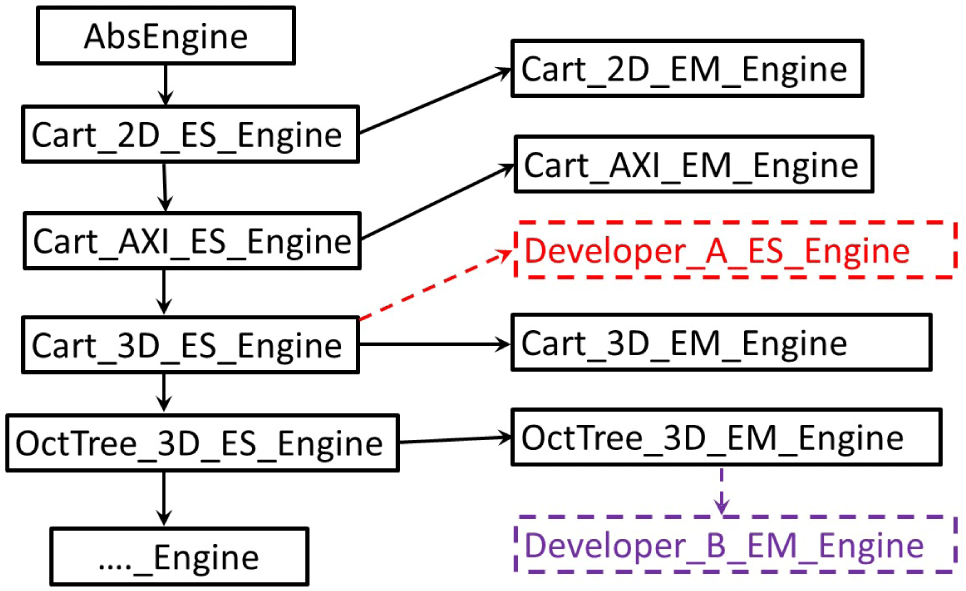
In this work, a C$++$ class named the ‘simulation engine’ is developed (Liu, Cai & Zou Reference Liu, Cai and Zou2012). It is introduced to organize different PIC related simulation schemes which can simulate different types of plasma flows. Essentially, this simulation engine class has the important ‘singleton’ (Gamma et al. Reference Gamma, Johnson and Vlissides1995) design pattern, which means only one object of this class is created in the package. This object is an abstract root class for all simulation schemes, serving the purpose of organizing difference classes. All the other simulation classes are daughter classes derived from this root class. Among these daughter classes, there are inherent internal relations. Figure 1 illustrates different simulation engine classes, or different plasma simulation schemes. This arrangement is effective, for example, it allows two or multiple developers to derive different classes for two different projects. As such, their work is independent, neither endangers/pollutes the basic class nor interferes with their colleagues’ classes. After they complete their projects, useful member functions and features in their classes can be summarized by their supervisor, incorporated or upgraded into the member functions in the mother classes. Evidently, the code architecture is open and convenient.

Benefiting from this simulation engine concept, the package can conveniently include many PIC simulation schemes. Examples include (i) three-dimensional plasma flows with Cartesian geometries; (ii) hybrid PIC schemes with the direct simulation Monte Carlo method (Bird Reference Bird1994) for plasmas with neutral gaseous species; (iii) full PIC schemes for electrostatic plasmas; (iv) full PIC schemes for electro-magnetic (EM) plasma flows. Theoretically, the package can include more functionalities without any difficulty. All these schemes have common functionalities, and they can be driven with a singleton object initialized from the abstract engine class.

Figure 1.

Illustrations of the inheritance relations among different simulation engine classes.

Figure 2.

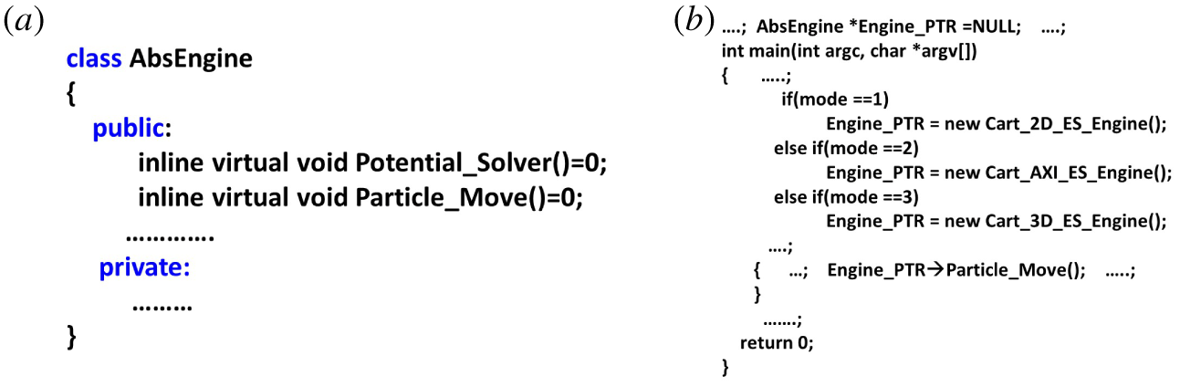
(a) Illustrations for a root class with pure virtual member functions; (b) the main code with the engine classes and objects.

All simulations performed with this simulation package are controlled by a file that includes many key parameters. This approach is the same as many standard commercial finite element analysis solvers, like NASTRAN (MacNeal Reference MacNeal1972), for computer aided engineering. These cards are scanned periodically while simulations continue, e.g. every 500 hundred steps. As such, users can modify the simulation parameters on the fly, there is no need to stop to read in new parameters and then restart the simulation from scratch again. The package writes out intermediate simulation results periodically and can restore the simulations by reading back the saved information.

Another novel feature of this root simulation engine class is that it adopts many pure virtual member functions that can effectively separate member functions’ names and interfaces. Two examples of such pure virtual member functions are shown in figure 2 with the unique programming grammar ‘$=0$’. As is well known, a standard class member function usually has four crucial elements: the function name, its parameter list, its function body and the return result type. However, a pure virtual member function cannot have a concrete function body. The sole purpose of such a pure virtual function is to define an interface for that member function in the mother and daughter classes. Those pure virtual functions for this abstract class of simulation engines are never called; instead, the corresponding immediate and derived daughter class’ true member function with a concrete function body is called during simulations. Figures 1 and 2(a) indicate the first daughter class ‘Cart_2D_ES_Engine’ derived from the root class with pure virtual functions must have a member function ‘Potential_Solver()’ with a concrete function body. All the other daughter classes from this ‘Cart_2D_ES_Engine’ may not need to implement a different member function body. If necessary, different member functions can be overridden inside a daughter class. A common issue for software packages with multiple schemes is the mixture of function interfaces and bodies. This implementation of pure virtual member functions efficiently resolves this issue, the interface is concise, and the corresponding maintenance work is convenient.

Figure 2(b) shows the main code which includes common interfaces shared by all daughter simulation engines. In one simulation, only one object for a specific daughter simulation engine class will be created, depending on a specific control card in the input file.

2.2 ES-PIC loop and data structure

A typical ES-PIC simulation procedure includes the following steps:

1. (i) select a simulation type, for instance, three-dimensional full kinetic ES-PIC;

2. (ii) choose whether to perform simulations on a serial or parallel platform, the latter needs to specify how many processors to run;

3. (iii) provide the mesh sizes and domain lengths along the $\text{X}-$, $\text{Y}-$ and $\text{Z}-$ directions;

4. (iv) specify other simulation parameters, e.g. inflow conditions, external fields, species information, time step size, boundary conditions, etc.;

5. (v) initialize the flow field;

6. (vi) compute the initial field(s);

7. (vii) enter the major loop and run for the pre-determined number of time steps; and

8. (viii) post-process.

A package user can conveniently change a simulation by modifying the specific card in the input file; hence, even a user without much knowledge of PIC schemes can perform a simulation.

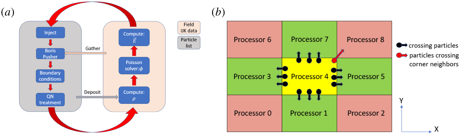
The data structure takes advantage of Cartesian mesh grids to separate particles and field data. Particle positions and velocities are stored in a single linked list for each species to allow continuous addition and removal of particles. The grid is Cartesian and it is straightforward to determine which cell a particle is located in. Field data are stored in an $IJK$ ordered array for fast access. Special gather and deposit functions are implemented to mediate information between the two data structures. The data structures and main loop are illustrated in figure 3(a).

Figure 3.

(a) Main loop and data structures for the simulation package; (b) two-dimensional illustration for transferring particles among sub-domains handled by different processors.

The main ES-PIC scheme class is derived from a standard PIC scheme class. With initial fields calculated, the code injects particles of different species into the simulation domain at the injection boundaries, where particle velocities are rewound by a half-time step to utilize the leap-frog scheme. The particle velocities and positions are advanced by a time step with the Boris pusher (Boris Reference Boris1970), and the advancements are based on the gathered local field values. The gathering process uses a second-order volume-weighting algorithm (Birdsall & Langdon Reference Birdsall and Langdon1991). The particle pusher has three modes: non-relativistic, relativistic and mixed. Aiming to save computation cost, only the particles that have high enough speeds will be pushed with a relativistic effect. After being pushed, particles interact with boundaries if they cross them. Then the quasi-neutral module is followed, where a user can select boundary treatments to ensure charge continuity in the system. This step is crucial to the stability of a full kinetic PIC simulation. By default, this module does almost nothing, but a detailed discussion will be presented in the next section with test cases. In the next step, the particles allocate their charges to adjacent grid nodes by using the same weighting scheme as the previously mentioned gathering process. The final step in the main loop is a Poisson equation solver, which utilizes the grid charge information to solve for the potential fields. The performance of the Poisson equation solver is crucial to an ES-PIC simulation because it is called in every step. The code adopts the conjugate gradient method (Golub, Charles & Loan Reference Golub, Charles and Loan2012) for both serial and parallel computation modes. For the serial mode, the Poisson equation solver is pre-conditioned by using incomplete Cholesky factorization with zero fill (IC0). The parallel implementation of the solver is to be presented and discussed in the next section.

2.3 Parallel computation schemes

One issue which must be addressed is to choose the proper parallel scheme to implement the PIC scheme. One approach is to allocate particles evenly among multiple processors, regardless of their positions, to ensure balanced loads. However, because particles need local field information, which may be stored by another processor, the related communication cost is high. Another more popular approach divides the physical simulation domain into many sub-domains to be handled by different processors. Each processor handles a specific sub-domain field, which is further used to push particles located in this sub-domain. The second approach is adopted in this package for parallel computations because it is straightforward to implement with superior performance (Blahovec et al. Reference Blahovec, Bowers and Luginsland2000; Wolfheimer, Gjonaj & Weiland Reference Wolfheimer, Gjonaj and Weiland2006). A defect of this approach is that particles may travel across different or even multiple sub-domains, thus transferring particles among processors is needed. The package adopts the message passing interface (MPI) method to communicate messages among processors, due to the good scalability and availability in most high performance computation facilities.

The parallel ES-PIC loop treatments are the same as those for a serial computation mode except for two issues that need special attention. One issue is particle movements. Particles entering the neighbouring sub-domains must be handed over to another processor. The other issue is about the Poisson equation solver, where ghost layer information must be communicated during each iteration. Those information exchanges across different sub-domains are handled by different processors. The treatments for these two issues are discussed in what follows.

3.1 Test Case I: a positive probe in non-drifting magnetized plasma

We first perform a series of simulations with a positive probe immersed in non-drifting magnetized plasmas. The probe potential ranges from 5 to 40 V. We then compare the simulated current collection with the values predicted by the Parker & Murphy (Reference Parker and Murphy1967) theory. Parker and Murphy considered the conservation of canonical angular momentum of an electron in a cylindrically symmetric force field, and derived an upper limit for the collected current by the positive probe

(3.1)$$\begin{eqnarray}I_{PM}=2\unicode[STIX]{x03C0}{r_{0}}^{2}j_{0},\end{eqnarray}$$

where $r_{0}$ is the maximum radius from which current can be collected, and $j_{0}$ is the electron thermal current in the plasma. The relation between $r_{p}$ and $r_{0}$ is given as

(3.2)$$\begin{eqnarray}r_{0}^{2}/{r_{p}}^{2}\leqslant 1+(8\unicode[STIX]{x1D6F7}_{0}/(m_{e}{\unicode[STIX]{x1D714}_{e}}^{2}{r_{p}}^{2}))^{0.5},\end{eqnarray}$$

where $\unicode[STIX]{x1D6F7}_{0}$, $m_{e}$ and $\unicode[STIX]{x1D714}_{e}$ denote electron potential energy, electron mass and electron cyclotron frequency respectively.

Figure 4.

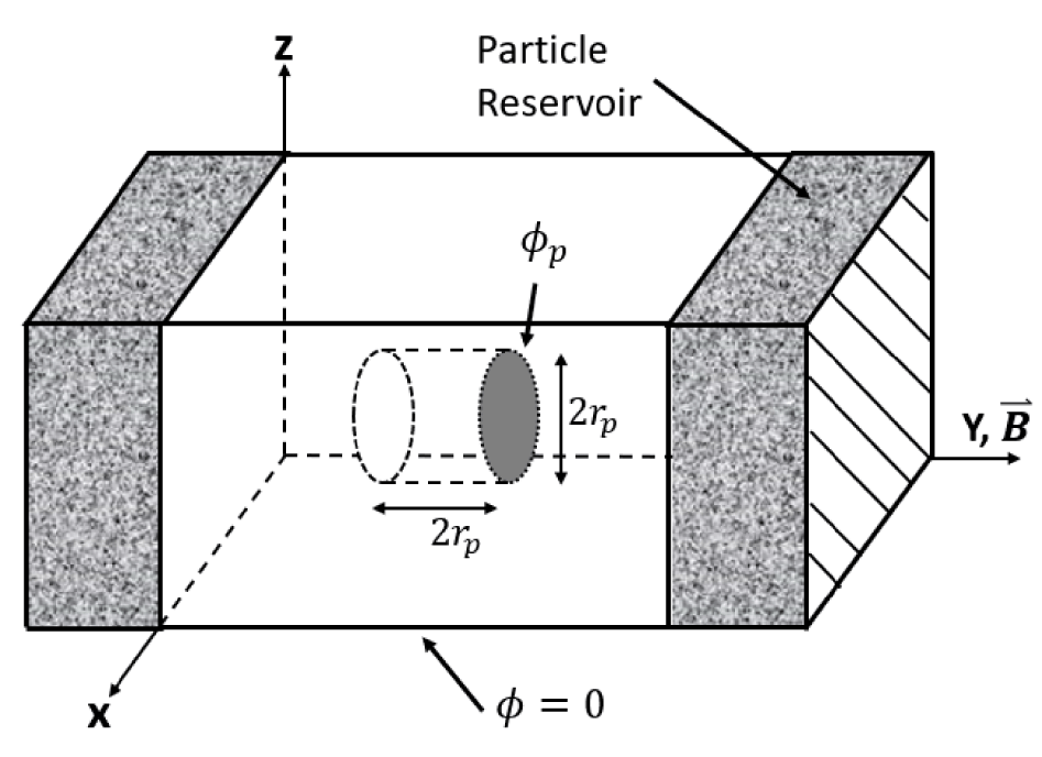
Test Case I: simulation set-up. Domain size: $\text{NX}=\text{NZ}=157$, $\text{NY}=221$, where NX, NY, NZ denote the number of nodes along each axis; mesh size $\unicode[STIX]{x0394}x=\unicode[STIX]{x0394}y=\unicode[STIX]{x0394}z=0.0105~\text{m}$, approximately one Debye length.

The simulation set-up is illustrated in figure 4. The following plasma parameters are used in this test case: ambient plasma density $n_{0}=1\times 10^{11}~\text{m}^{-3}$, the ion to electron mass ratio $m_{i}/m_{e}=100$, magnetic field $B_{y}=0.3~\text{G}$, the ratio of probe radius to Debye length $r_{p}/\unicode[STIX]{x1D706}_{D}=15$, electron and ion temperatures $T_{e}=T_{i}=0.2~\text{eV}$. With these parameters, the electron and ion gyro-radii are approximately $0.34r_{p}$ and $3.38r_{p}$, respectively. A small ion to electron mass ratio is used to accelerate the simulations. Additional tests are performed with a bigger ion to electron mass ratio, while the electron gyro-radius is the same. These tests confirmed that the smaller mass ratio treatment does not change the collected currents.

Test Case I uses similar parameters and treatments to the work done by Singh et al. (Reference Singh, Vashi and Leung1994). Singh placed particle reservoirs at each magnetic end of the simulation domain. As such, electrons and ions can move into the simulation box; there is no need to compute the precise entrance angles. The reservoir contains equal numbers of ions and electrons, both with Maxwellian velocity distributions. At the beginning of each time step, randomly positioned particles leave the reservoir and enter the simulation box. After each time step, the reservoir is randomly refreshed to maintain enough particle sources. The reservoirs are connected to two of the cubic simulation box faces, whose normal directions are parallel to the magnetic field. As such, the entering electrons can move along the magnetic field lines and fill the simulation box quickly. It is feasible to put reservoirs on the remaining four simulation domain faces as well, but such a treatment can increase the computational cost. Boundary treatments are needed to preserve electrons exiting the boundary faces that have no reservoirs attached. This is because electrons have gyro-motions and can exit and re-enter the boundary faces frequently. In the computation, an exiting electron is simply deleted from the simulation if no treatment is performed. This can be improved by setting those boundaries to be reflective, or simply by re-injecting those escaped electrons into the simulation domain.

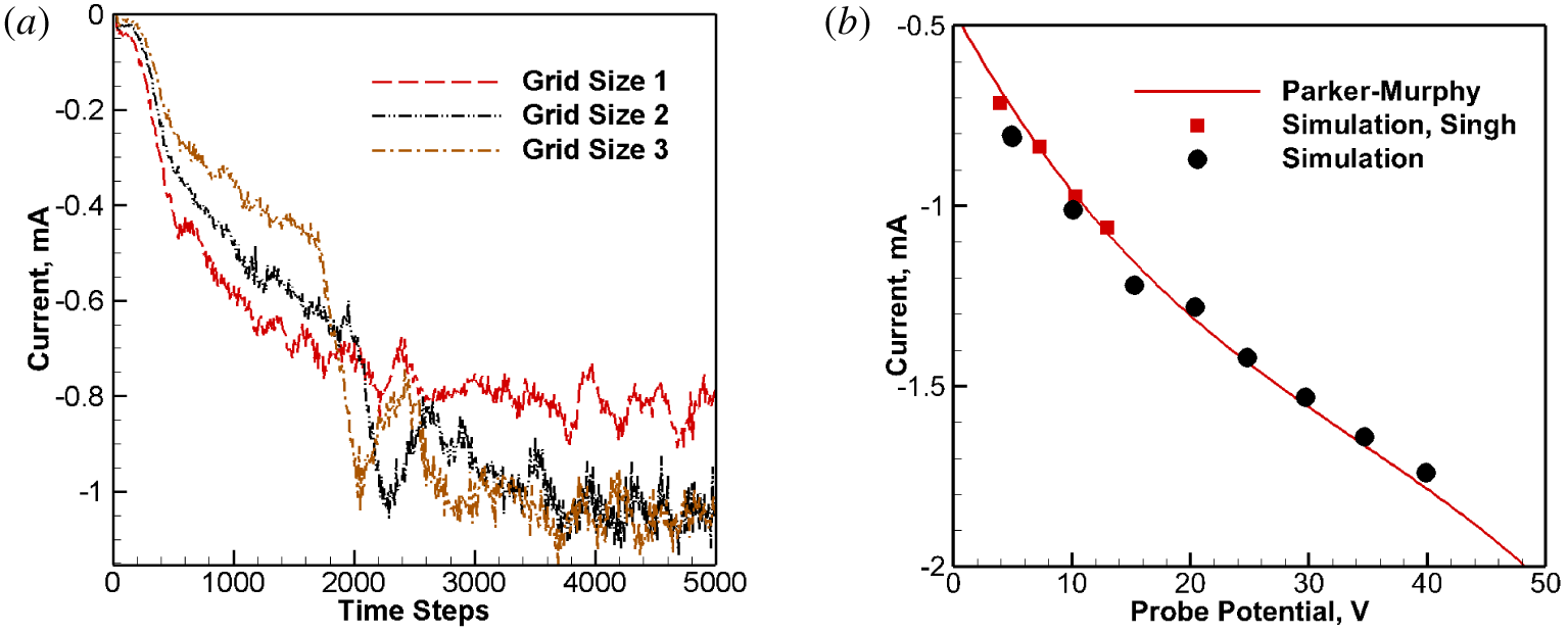
The simulation was performed with 96 processors, 5000 time steps and lasted approximately 34 min. Figure 5(a) shows the current collecting history for the 10 V probe potential case. Three different grid sizes were used to confirm grid convergence, where Grid Set 2 with a mesh size 0.0105 m is adopted for our final simulations, while Grid Sets 1 and 3 are coarser and finer, respectively. The time-averaged current value in the steady state is approximately 1.1 mA, very close to the value of 0.980 mA which is predicted by the Parker–Murphy theory. Figure 5(b) shows the current–voltage curve over a range of different probe potentials. The solid line is from asymptotic values predicted by the Parker–Murphy theory. The triangles represent our PIC simulation results, and the squares represent the results obtained by Singh. It should be mentioned that, in Singh’s work, they used a mesh in a cylindrical coordinate system, while in our work, we used a cubic mesh. The former can fit a spherical probe surface with higher accuracy, and we believe this is the reason why their results have relatively better agreement compared to our results. However, as shown, the good agreement among the three sets of data indicates that our PIC package implementations are still reliable.

Figure 5.

Test Case I: (a) probe current collection history for the case of 10 V probe surface potential; (b) the I–V relation predicted by the Parker–Murphy theory and simulations.

3.2 Test Case II: unmagnetized space charges collected by a spherical probe

In this test case, we use the theoretical result by Laframboise (Reference Laframboise1966) to validate our code. Laframboise’s theoretical study solves the Poisson–Vlasov equation for electrons. The method computes the electron densities at special points in the distribution function, and this distribution function is determined by the conservation of angular momentum and energy. A nonlinear system of integral equations were derived and solved numerically to obtain the current collections by the positive probe. Unlike the first test case, there is no magnetic field, and the probe shape is spherical. The same as Case I, our simulation domain adopts cubes. The plasma parameters are the same for the previous test case except the probe radius $R_{p}$ are used. We perform two series of simulations, with $r_{p}/\unicode[STIX]{x1D706}_{D}=5$ and 10. The simulation technique is similar to Case I except the reservoirs are attached to every boundary face. This is because without a magnetic field, particle collections do not have favourable directions.

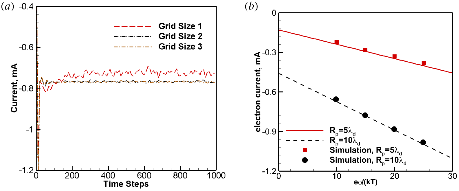
The simulation is performed with 96 processors, 1000 time steps and lasts approximately 9 min. Figure 6(a) shows the electron current collection history for one series of simulations with $R_{p}=10\unicode[STIX]{x1D706}_{D}$. Three different grid sizes were used to show grid convergence. Grid Set 2 with a size of 0.0105 m is chosen for simulations, while Grid Sets 1 and 3 have double or half the size. As seen from figure 6(a), the simulation reaches steady states relatively faster with smaller fluctuations when compared with Case I, which has an external magnetic field. Figure 6(b) shows that our simulation results agree well with Laframboise’s theoretical results. Since our code adopts Cartesian meshes, the spherical probe is approximated by cubes. A total of 157 mesh points are used along the X, Y and Z directions and the mesh sizes are close to one Debye length. This explains why, in figure 6(b), the results for the larger probe scenario, $R_{p}=10\unicode[STIX]{x1D706}_{D}$, show better agreement than the smaller probe case: the spherical probe is better approximated by using more mesh points.

Figure 6.

Test Case II: (a) electron current development history for probe $R_{p}=10\unicode[STIX]{x1D706}_{D}$, $e\unicode[STIX]{x1D6F7}/kT=15$ and $T_{i}/T_{e}=1.0$; (b) electron current collections: simulation (symbols) and Laframboise’s theoretical (lines) results.

4.1 Case III: a positive probe in an $\boldsymbol{E}\times \boldsymbol{B}$ drifting magnetized plasma

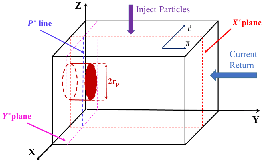
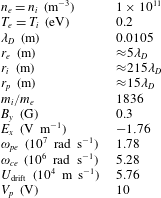
Case III was investigated by Singh et al. (Reference Singh, Leung and Vashi1997). The simulation parameters are listed in table 1, and figure 7 illustrates the simulation set-up. Also shown in the same figure, the external magnetic field is along the Y-axis with a magnitude of 0.3 G, and the external electric field along the negative X direction is set to be $1.728~\text{V}~\text{m}^{-1}$. A relative motion of $0.3V_{th,e}$ or $13V_{th,i}$ between the plasma and simulation box is created, where $V_{th,e}$ and $V_{th,i}$ are the electron and ion thermal velocities respectively. This flow regime is characterized by $r_{e}<r_{p}$, $r_{i}\gg r_{p}$ and $\unicode[STIX]{x1D714}_{pe}>\unicode[STIX]{x1D714}_{ce}$, where $r_{e}$, $r_{i}$, $r_{p}$, $\unicode[STIX]{x1D714}_{pe}$ and $\unicode[STIX]{x1D714}_{ce}$ are gyro-radii of electrons and ions, probe radius, plasma frequencies and electron gyro-frequencies respectively. Ions in this flow regime are effectively un-magnetized due to the large gyro-radius to probe radius ratio.

Figure 7.

Case III: simulation domain illustration. Domain size: $\text{NX}=\text{NZ}=157$, $\text{NY}=289$, where NX, NY, NZ denote the number of nodes along each axis; mesh size $\unicode[STIX]{x0394}x=\unicode[STIX]{x0394}y=\unicode[STIX]{x0394}z=0.01~\text{m}$.

Table 1.

Simulation parameters for Case III (Singh et al. Reference Singh, Leung and Vashi1997).

For convenience, two special planes and one line are defined to aid result discussions for the last two test cases. The $X^{\ast }$ plane is defined as the plane with a fixed X value, it is normal to the $\text{X}$-axis and passes the probe centreline. The $Y^{\ast }$ plane is defined as the one perpendicular to the probe centreline, and it evenly bisects the extruded probe, i.e. $y=R_{p}/2$. The $p\ast$ line is the intersection line formed by these two planes.

The simulations adopted the following parameters: mesh size $\text{d}x=\text{d}y=\text{d}z=0.01~\text{m}$, which is approximately one Debye length; time step $\unicode[STIX]{x0394}t=3.56\times 10^{-8}~\text{s}$. The simulation begins with a plasma flow being injected from the top boundary face. It drifts downward and eventually leaves the simulation domain from the bottom boundary face. The left boundary face (i.e. $Y=0$) connected to the probe is set up as a symmetric plane to reduce the simulation cost. A symmetric plane means that when a particle hits it from the domain, it will not be removed from the simulation; instead, it bounces back into the simulate domain, with its normal velocity components reversed but its parallel velocity components unchanged. We compare the results with those from cases without such a symmetric plane treatment and confirm that the symmetry boundary is valid and can reduce the computation cost by half. Particles can also exit from the other four boundaries and be deleted from the simulations. The electrostatic potential is updated every time step by solving Poisson’s equation and the gradients are adopted to update the electric field in the simulation box. All boundary faces adopt a Dirichlet boundary condition with a zero potential, except that the left boundary face adopts a Neumann boundary condition $\unicode[STIX]{x2202}\unicode[STIX]{x1D719}/\unicode[STIX]{x2202}n=0$ due to the symmetry. The probe surface potential is set to 10 V.

To sustain a stable simulation, the system neutrality requirement must be maintained. The injection introduces an equal number of electrons and singly charged ions to establish a plasma flow into the simulation box, at a rate calculated by: $U_{\text{drift}}\boldsymbol{\cdot }\boldsymbol{n}\,\text{d}t\,\text{d}s$. However, because lighter electrons have higher velocities, they usually exit the simulation boundaries with a much higher rate than ions. As consequence, the simulation boundaries change to charge positive and further exacerbate the simulations. Another source of electron depletion is from the current collecting probe. A positive probe continues to collect electrons in the simulation and causes the system to be positively charged. In this test case, we adopt Singh’s treatment, where those particles leaving the boundary faces are rejected back to the simulation box boundary faces; and those electrons collected by the positive probe are returned to the system at the right boundary facing the probe end. In this case, we did not adopt the reservoir treatments (i.e. with extra buffer volumes outside the simulation domains) which were used in Cases I and II. The simulation is performed with 96 processors, 2000 time steps and lasts approximately 3 h. With those flow parameters, the plasma flow takes approximately 700 time steps to reach the bottom boundary; hence, the simulation has sufficient time to reach a steady state.

Figure 8.

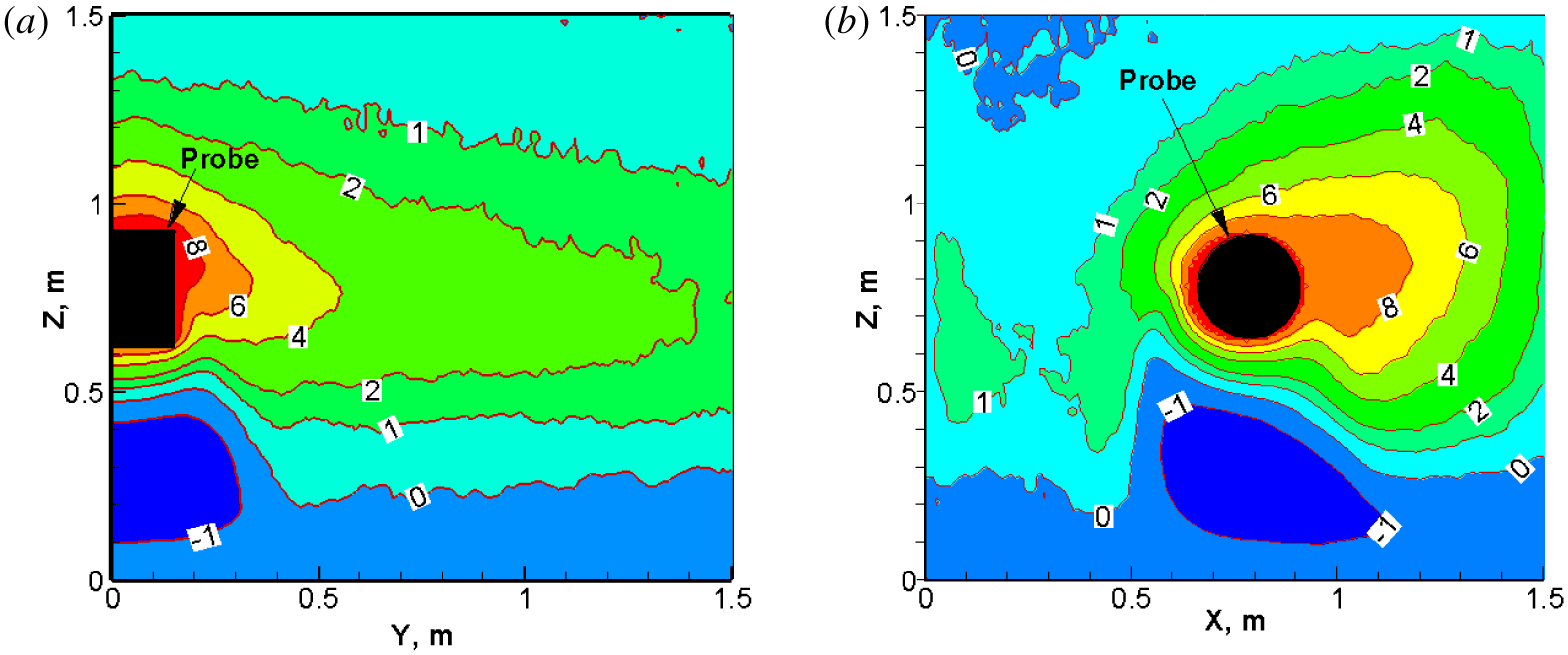
Case III: potential (units: Volt) contours in the (a) $X^{\ast }$ plane; and (b) $Y^{\ast }$ plane. Probe surface potential: 10 V.

The simulation results are very close to those obtained by Singh et al. (Reference Singh, Leung and Vashi1997), with several slight differences. This is due to subtle implementation details, e.g. different types of meshes.

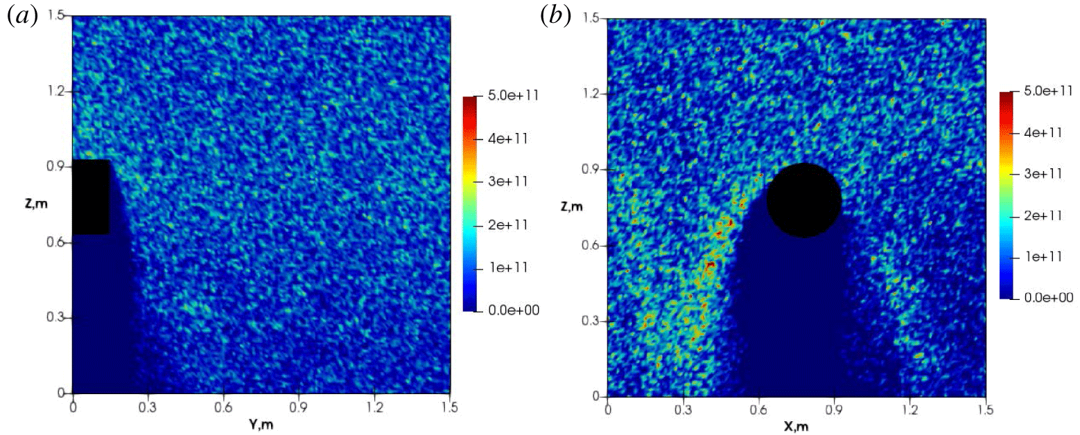
Here, we briefly discuss the flow field characteristics and offer several implementation recommendations to simulate $\boldsymbol{E}\times \boldsymbol{B}$ drifting plasma flows around a positive probe with similar parameters. We first discuss the potential sheath structures near the probe. Figure 8 shows the potential contours inside the $X^{\ast }$ and $Y^{\ast }$ planes. Figure 8(a) shows that the sheath structures extend much further along the magnetic field direction and bend towards the wake region. Figure 8(b) demonstrates fan-shape structures around the probe with a negative potential wake region. These observations are consistent with the previous simulation results obtained by Singh et al. (Reference Singh, Leung and Vashi1997). The negative potential in the wake is mostly due to the absence of ions in that region, and it is well illustrated by figure 9. On the other hand, electrons can enter the wake region even with the obstructions from the probe, as shown in figure 10. Both the potential structure and species density profile display asymmetry patterns in the $Y^{\ast }$ plane, due to the presence of magnetic field.

Figure 9.

Case III: snapshots of ion number density $n_{i}$ in the (a) $X^{\ast }$ and (b) $Y^{\ast }$ planes. Unit: $\text{m}^{-3}$. Ions are expelled from the probe and have difficulty entering the wake region.

Figure 10.

Case III: snapshots of electron number density $n_{e}$ in the (a) $X^{\ast }$ and (b) $Y^{\ast }$ planes. Unit: $\text{m}^{-3}$. They are attracted to the probe and can enter the wake region.

Figure 8(b) illustrates the potential patterns, and it is evident that the lower-left region has larger gradients than the lower-right region. As such, the corresponding left wing is more effective in blocking ions and forms a slightly higher ion accumulation region than the right side. This result is correctly shown in figure 9(b). Due to the same reason, the left lower region of the probe can attract more electrons than the right lower region, this fact is also correctly illustrated by figure 10.

Figure 11.

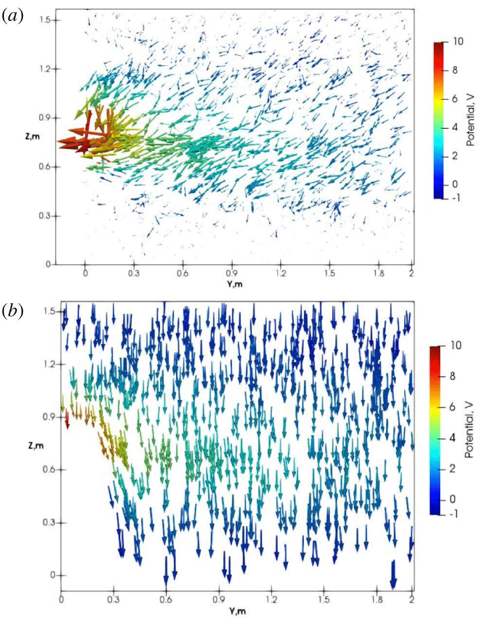
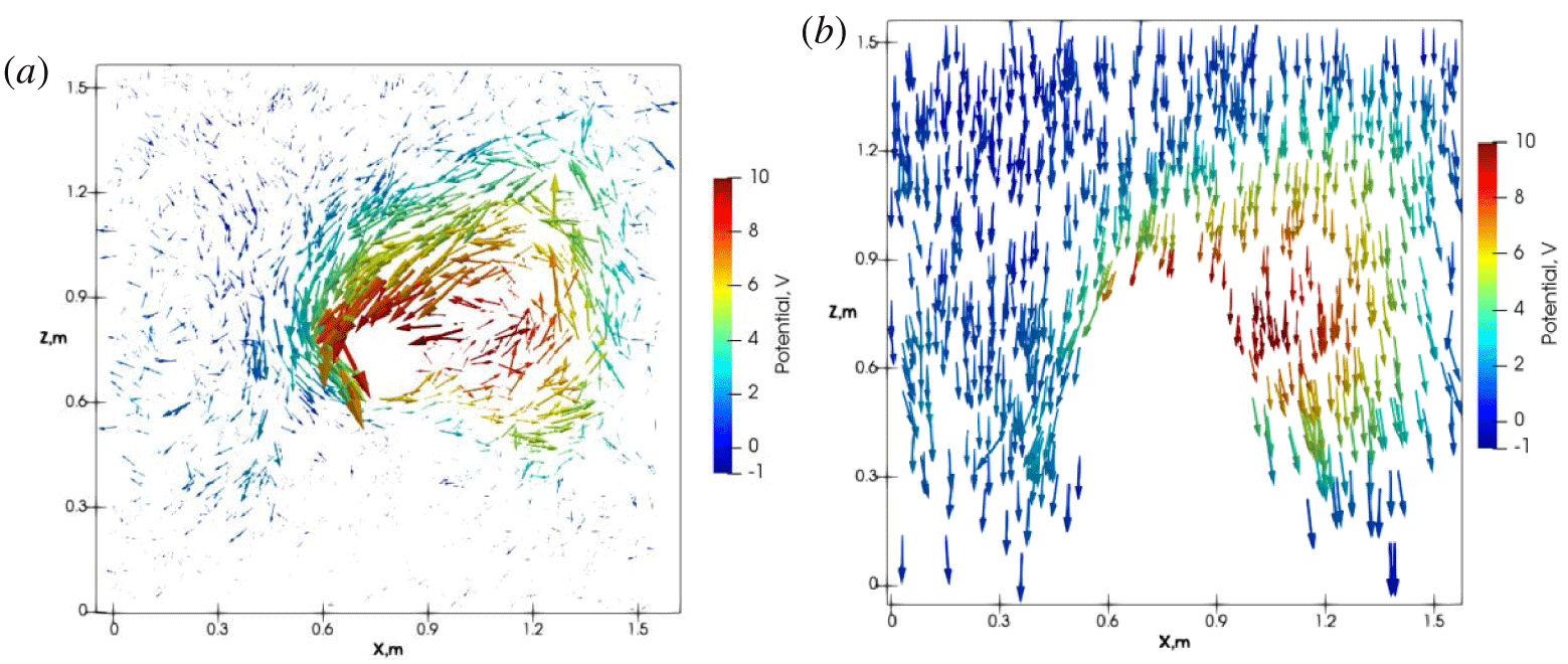
Case III: (a) electron velocity vectors in the $X^{\ast }$ plane, averaged over 30 time steps; (b) the corresponding ion velocity vectors in the same plane.

The ion and electron flow patterns are quite different. Figures 11 and 12 show the electron and ion velocity vectors inside the $X^{\ast }$ and $Y^{\ast }$ planes. These vectors are coloured by electric potential magnitude to help illustrate the potential sheath effects. Vector plots for electrons are averaged over 30 time steps to reduce the randomness caused by electron gyro-motions. In both planes, the ion flows are mostly unaffected by the probe and magnetic fields, which is expected because ions are not magnetized with the given simulation parameters. Essentially, ions drift downward and only divert away from locations very close to the probe with strong electric fields. The electrons, on the other hand, are strongly influenced by the probe and magnetic fields. Parallel to the magnetic fields, the electric field accelerates electrons towards the probe, as shown in figure 11(a). In the $X^{\ast }$ plane, ions are less affected in the potential sheath region, as shown in figure 11(b). This explains that the extended potential sheath along the magnetic field is due electron depletion in this region. In the $Y^{\ast }$ plane, figure 12(a) shows that electrons experience strong circulating forces around the probe, due to the local radial electric field and the resulting local $\boldsymbol{E}\times \boldsymbol{B}$ drifting effect. This circulation zone has a large cross-sectional area with asymmetrical features. Figure 12(b) shows the corresponding ion flow vectors in the $Y^{\ast }$ plane. Ions have local $\boldsymbol{E}\times \boldsymbol{B}$ drift motions as well, but only near the left side of the probe. This is convenient to understand, because the external convection electric fields point to the negative X-axis direction, the local down-drift on the left side of the probe is combined with the external electric field at the same side. On the right side of the probe, however, the local drifting effects must counteract the large downward drift, and less ions stay in that area.

Figure 12.

Case III: (a) electron velocity vectors in the $Y^{\ast }$ plane, averaged over 30 time steps; (b) the corresponding ion velocity vectors in the same plane.

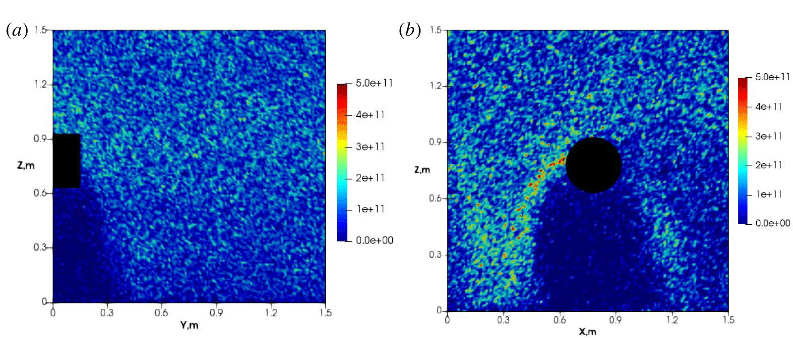
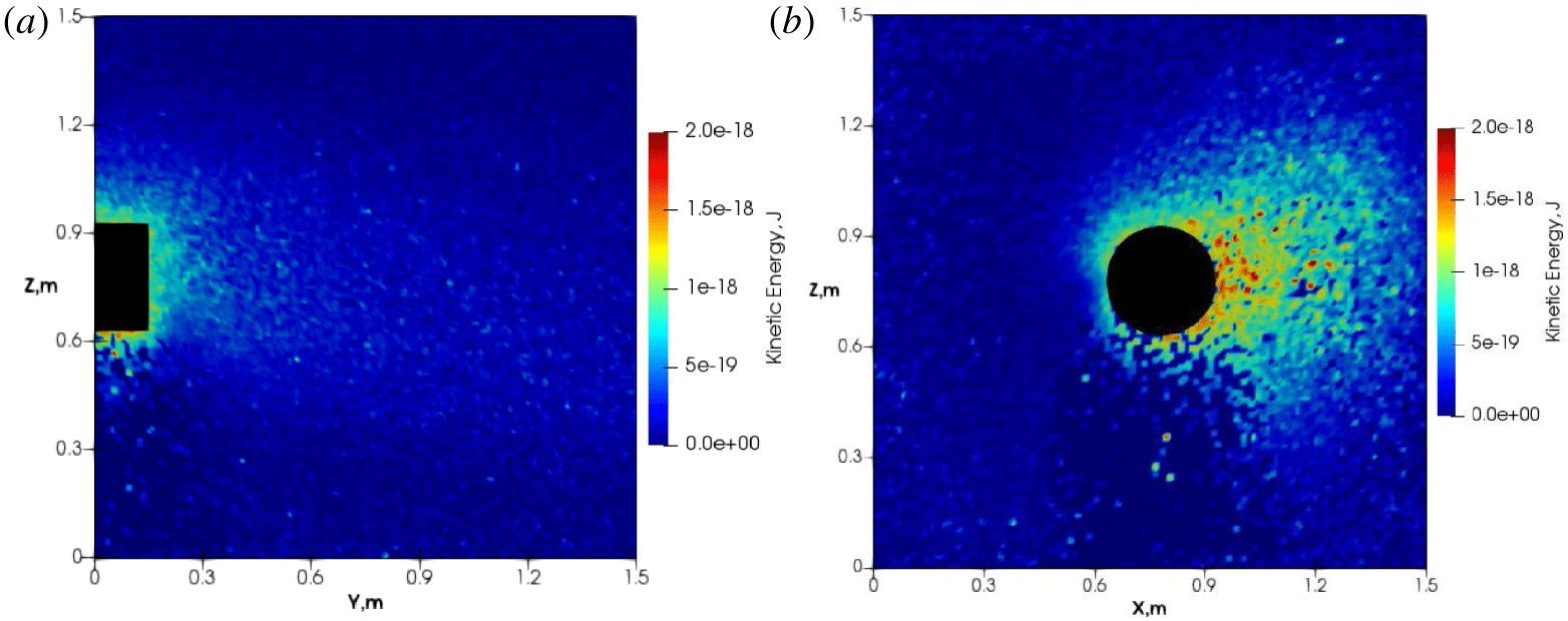
Particles are heated near the probe in the potential sheath region, especially electrons. Figure 13 presents the electron kinetic energy inside the two planes. In the $X^{\ast }$ plane, electrons gain kinetic energy when they enter the potential sheath, forming a high kinetic energy zone, shown as figure 13(a). In the $Y^{\ast }$ plane perpendicular to the magnetic field, there are electrons with high speeds around the probe, as shown in figure 13(b). Electrons around the probe gain a sufficiently high energy to circulate around the probe, counter-acting the downward drifting motions. We recall that the downward drifting velocity is around $0.3V_{th,e}$, thus it is easier for high energy electrons to move upwards even with the external downward $\boldsymbol{E}\times \boldsymbol{B}$ drifting velocity. Figure 13(b) also shows that high energy electrons are present near the boundary faces, at the right boundary face, i.e. the electrons circulating zone near the probe, electrons constantly deplete. These observations recommend that the simulation box should have a larger mesh size along the X direction.

Figure 13.

Case III: electron kinetic energy in the (a) $X^{\ast }$ and the (b) $Y^{\ast }$ planes.

Figure 14.

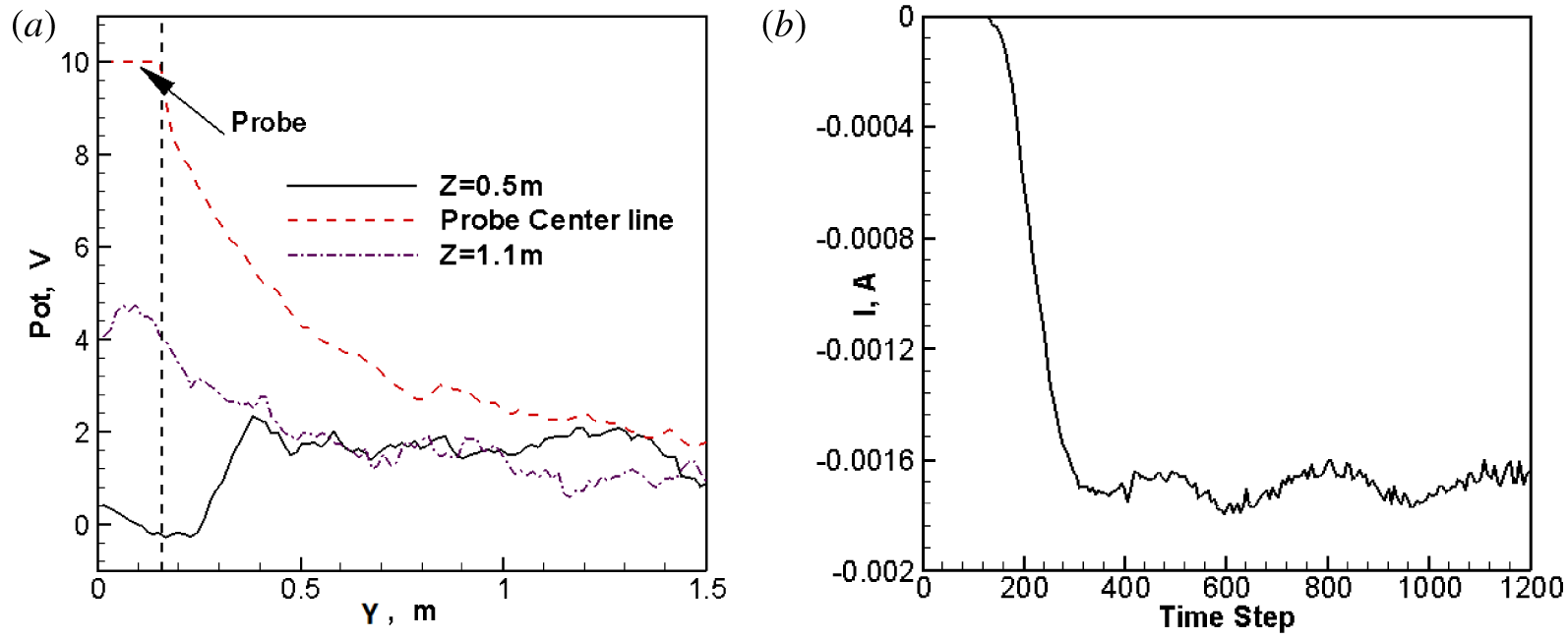
Case III: (a) averaged potentials extracted along $Z=0.5~\text{m}$, probe centreline $Z=0.0~\text{m}$ and $Z=1.1~\text{m}$, at a final quasi-steady flow state; (b) collected current development history.

Figure 14(a) shows three potential profiles extracted from three lines: $Z=0.5~\text{m}$ (below the probe), $Z=1.1~\text{m}$ (in the ram side) and along the probe centreline $Z=0.0~\text{m}$, at a final quasi-steady state. A significant portion of the last profile passes through the high potential sheath region. In the ram side above the probe, the potential rises and gradually drops along the magnetic lines, as shown with the $Z=1.1~\text{m}$ line. In the wake region, where only electrons exist, the potential is low and eventually rises to the regular potential value along the magnetic field direction, as shown with the $Z=0.5~\text{m}$ line. These lines eventually reach similar potential values at a location of approximately $Y=1.5~\text{m}$.

Figure 14(b) shows the probe current collection development history. The current slightly oscillates but in a quasi-steady state, so it indicates that our boundary treatments are proper for establishing quasi-neutrality in the simulations. As such, the above results are reliable. The collected current is around 3.4 mA ($1.7~\text{mA}\times 2$ since we only simulate half of the domain), which is larger than the 2.1 mA obtained from Singh’s simulations. We have performed several tests with different mesh sizes, simulation domain sizes, macro–real particle ratios, etc., and all the results converge to the save value of 3.4 mA. The discrepancy may come from several subtle implementation differences. First, we adopt a uniform Cartesian grid with a mesh size smaller than one Debye length. In comparison, Singh adopted a non-uniform cylindrical mesh with a largest mesh size of 10 Debye length at the boundaries. In addition, the simulation box in our study is cubic with six boundary faces. Singh’s simulation domain is a large cylinder with four boundary faces. Most likely due to these reasons, their past results are inferior. Lastly, there are many minor implementation differences, e.g. the random number generator can impact the statistical behaviours of the plasma flows.

Figure 15.

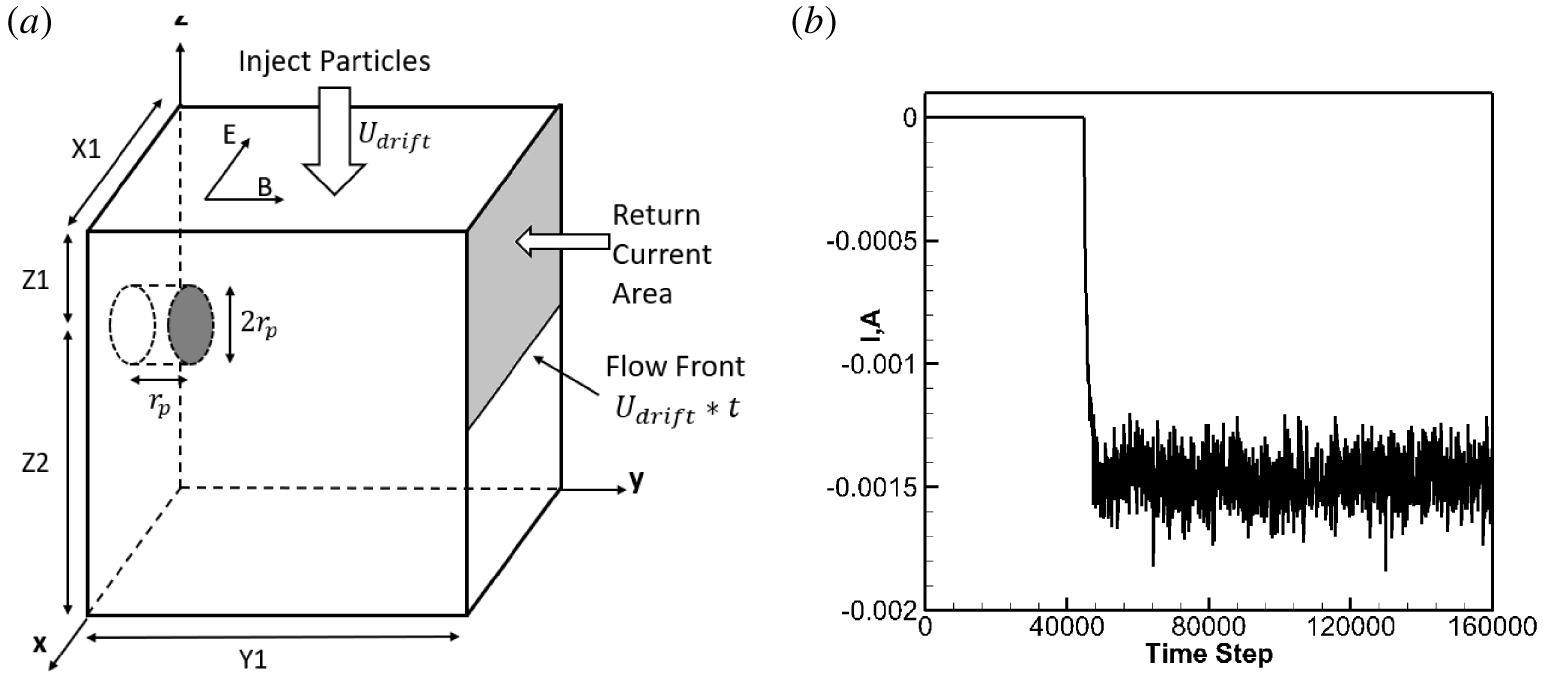
Case IV: (a) simulation domain illustration, $X1=90\unicode[STIX]{x1D706}_{D}$, $Y1=300\unicode[STIX]{x1D706}_{D}$, $Z1=40\unicode[STIX]{x1D706}_{D}$, $Z2=100\unicode[STIX]{x1D706}_{D}$; (b) probe current collection history.

Table 2.

Simulation parameters for test Case IV (Heinrich & Cooke Reference Heinrich and Cooke2013).

4.2 Test Case IV: a positive probe in an $\boldsymbol{E}\times \boldsymbol{B}$ drifting under-dense plasma

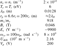
The last test case is the same as one past study (Heinrich & Cooke Reference Heinrich and Cooke2013). It is an under-dense plasma flow over a positively charged probe which is characterized by: $r_{e}<r_{p}$, $r_{i}<r_{p}$ and $\unicode[STIX]{x1D714}_{pe}<\unicode[STIX]{x1D714}_{ce}$. Different from Test Case III, ions are strongly magnetized in this case. Table 2 presents the flow parameters, and the simulation domain is illustrated in figure 15(a).

In this case, we do not adopt the reservoir treatment as used in Cases I and II. Several simulation techniques are similar to Case III, and a few of the differences are listed as follows.

Firstly, two side boundary faces connected to the symmetric plane, i.e. $X=0$ and $X=X1$, are set to be periodic. This treatment means there is a row of positive probes, and the major goal of such a treatment is to reduce the complex boundary condition effects. Both ions and electrons have gyro-motions due to the strong magnetic field, and they exit from one of these two boundary faces and re-enter the other boundary face frequently. By setting these two boundaries to be periodic, the neutrality condition is conveniently satisfied. Neumann boundary conditions for Poisson’s equation, $\unicode[STIX]{x2202}\unicode[STIX]{x1D719}/\unicode[STIX]{x2202}n=0$, are adopted for all the boundary faces except for the top face. We have attempted to implement the Dirichlet boundary conditions as used in Test Case III, but the Neumann boundary conditions illustrate superior stability in this test case.

Figure 16.

Case IV: (a) $n_{i}$, (b) $n_{e}$, in the $X^{\ast }$ plane. Unit: $\text{m}^{-3}$.

Secondly, the neutrality scheme is different from Case III. There is no particle loss at the two periodic boundary faces; thus there is no need for extra treatments. The symmetric face is still used to return the collected electrons. Because this face has a large size along the Z- direction, if the complete face area is used to return the collected particles, most electrons simply leave the bottom boundary later due to their large downward drifting motions, and this is not efficient. Instead, we allow the electron collection front to develop naturally with time. This is achieved by using a plasma front-marching surface moving downward with the drifting velocity, as shown in figure 15(b). The simulation is performed with 96 processors, and it lasts 39 hours with 160 000 time steps.

Figure 15(b) shows the current collection development history. As shown, after a certain simulation step, a relatively steady stage is reached with small current fluctuations. The collected current is approximately 3 mA ($1.5~\text{mA}\times 2$), close to the predicted value of 4 mA by Heinrich & Cooke (Reference Heinrich and Cooke2013). The small difference is because Heinrich adopted the entire right boundary face to inject electrons into the simulation box, resulting in enhanced electron collections parallel to the magnetic field. The defect of this treatment is that the simulation system may end up with more electrons than ions, and it breaks down the system quasi-neutrality with numerical errors.

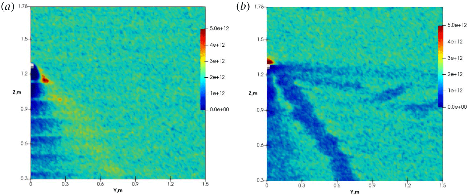
Figure 16(a,b) presents the ion and electron number density distributions in the $X^{\ast }$ plane. The positive probe is located at approximately $Z=1.27~\text{m}$ with a small diameter of 0.0254 m. Figure 16(a) shows that the ion flows form two distinctive patterns passing through the positive probe: a wake region and an ion-rich wing. The wing is formed due to the strong parallel electric fields near the probe, and it expels ions away from the probe. The ion-rich wing has a number density as high as 2.5 times the injecting plasma density immediately downstream of the probe, and the plasma flow gradually dissipates further downstream. Figure 16(b) shows the electron flow patterns in the same plane with several evident flow patterns. First, an electron trapping region appears around the probe with a number density as high as 5.5 times the injecting plasma density. Second, an electron depletion wing parallel to the magnetic fields along the Y axis emerges. Finally, a wake region and another electron depletion wing are present in the ion-rich wing region. These flow patterns are consistent with the results by Heinrich & Cooke (Reference Heinrich and Cooke2013), except the second electron depletion wing is in the ion-rich wing region. These discrepancies only appear in the combined charge density profile, and only net positive charges are visible in the ion-rich wing region, obscuring the presence of an electron depletion region. The related plasma physics is rather complex and we confirm their work and recommend their paper (Heinrich & Cooke Reference Heinrich and Cooke2013) for detailed explanations.

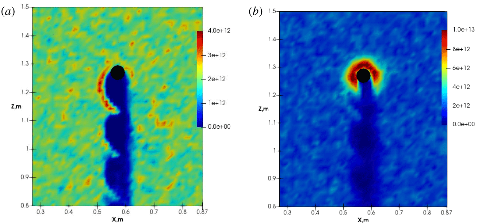
Figure 17(a,b) presents ion and electron number density profiles in the $Y^{\ast }$ plane. For both species, the repeating wake patterns are similar, indicating that they are caused by the local $E\times B$ drifting effect. The magnetic field is along the positive Y-axis, which is perpendicular to the paper and leaving the reader. The strong local radial electric field causes both species to accumulate around the probe, counter-clockwise with the presence of the strong external magnetic field. Figure 17(a) further shows that the wake is asymmetric. On the left side of the probe, the wake shows evident wave patterns, while on the right side, no clear wave patterns are visible. This is due to the fact that the external convection electric field is along the $\text{X}$-axis direction (pointing from right to left), and the local electric field counteracts the external electric field at the right side of the probe. Figure 17(b) highlights electron trapping regions around the probe.

Figure 17.

Case IV: (a) $n_{i}$ and (b) $n_{e}$ in the $Y^{\ast }$ plane. Unit: $\text{m}^{-3}$.

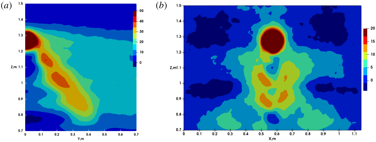
Figure 18(a,b) shows potential profiles. The high probe potential is well confined within a small region. Figure 18(a) shows the potential structures in the $X^{\ast }$ plane, and the positive potential region coincides with the ion-rich wing region. The potential structure extends along the magnetic field due to electron depletion, similar to test Case III. Figure 18(b) shows the potential structures in the $Y^{\ast }$ plane. Unlike Case III, with a negative potential region in the wake, the overall potential behind the probe is slightly positive, because both ions and electrons are highly magnetized and can enter this region. The asymmetry patterns are not evident in this case.

Figure 18.

Case IV: potential contours in the (a) $X^{\ast }$ and (b) $Y^{\ast }$ planes. Unit: Volts.

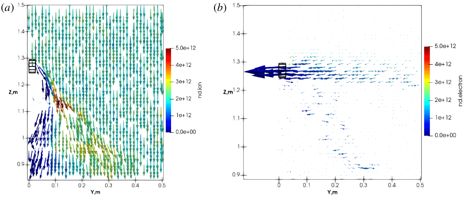
Figure 19 shows ion and electron velocity vectors in the $X^{\ast }$ plane. The vectors are scaled by the velocity magnitudes and coloured by their number densities. Figure 19(a) indicates two interesting areas, one is the ion-rich wing with light yellow colours, and the other is the wake region of ion flows, pointing to the left. The ion flow in the ion-rich wing points to the right is due to the expelling effect from the positively charged probe. The wake region flow pointing to the left is due to the existence of the ion-rich wing, which introduces a local left-pointing parallel electric field. Figure 19(b) shows the corresponding electron velocity vectors in this plane. Parallel to the magnetic field, electrons are easily collected and accelerated towards the probe due to their small mass, forming a current collecting tube. Another interesting feature is, in the ion-rich wing region, electrons accelerate along the parallel direction, due to the local parallel electric field created by the ion-rich wing.

Figure 19.

Case IV: (a) ion and (b) electron velocity vectors in the $Y^{\ast }$ plane, coloured by their number densities.

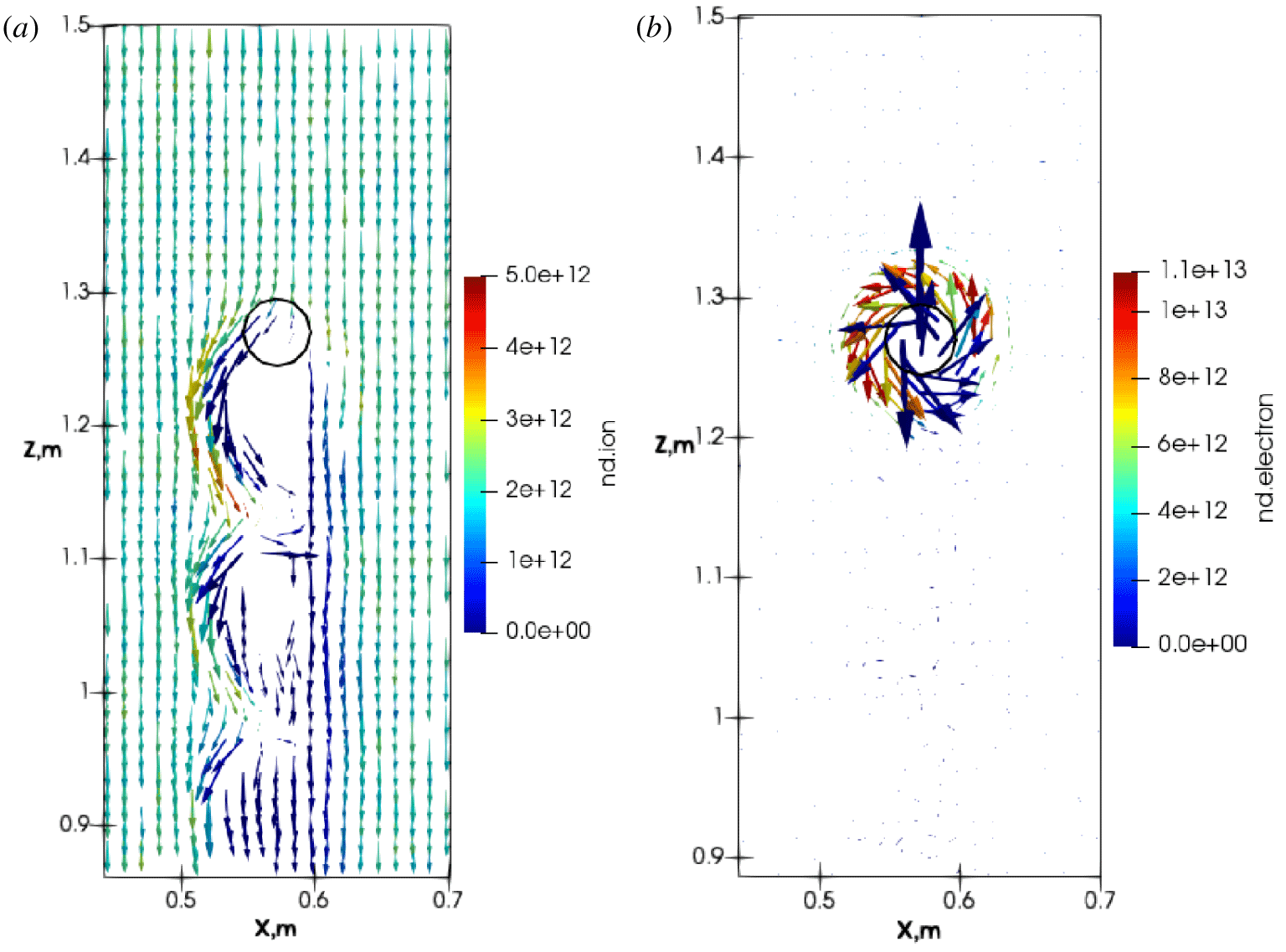
Figure 20(a,b) shows the velocity vectors for ions and electrons in the $Y^{\ast }$ plane. Ion flows are likely affected by both the local $E\times B$ drifts and the ion gyro-motions. To better illustrate the trapping effect around the probe, velocity vectors for electrons are calculated by first subtracting the downward drifting velocity caused by the external electric fields. The trapping region has a diameter two times larger than the probe diameter, and the electron number density is higher in this region, creating a shielding effect.

Figure 20.

Case IV: velocity vectors for: (a) ions, and (b) electrons, in the $Y^{\ast }$ plane. Coloured by their number densities; electron downward drift motions are removed to illustrate the trapping effect.

Figure 21.

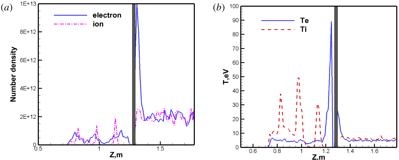
Case IV: (a) number density (unit: $\text{m}^{-3}$), and (b) average temperatures, along the $P^{\ast }$ line.

Figure 21(a,b) shows the ion and electron number densities and average temperatures, along the $P^{\ast }$ line. The grey bar represents the probe. The left side of the probe is the wake region, and the right side is the ram region. It can be seen from figure 21(a) that the electron number density rises near the probe on the ram side mainly because they impinge from the top and are attracted to the positive probe but ions are expelled from the probe; the overall electron number density is much higher than the ion number density. In the probe downstream wake regions, both species have lower number densities. Figure 21(b) shows the corresponding ion and electron average temperatures. In the wake, electrons have higher temperatures than the ions. There are three spikes in the average ion temperature profiles, which are consistent with the spikes in the corresponding ion density shown in figure 17(a), and ion velocities shown in figure 20(a). In the wake, the highest averaged electron temperature is approximately 90 eV, which is almost twice the highest ion temperature, of approximately 50 eV).

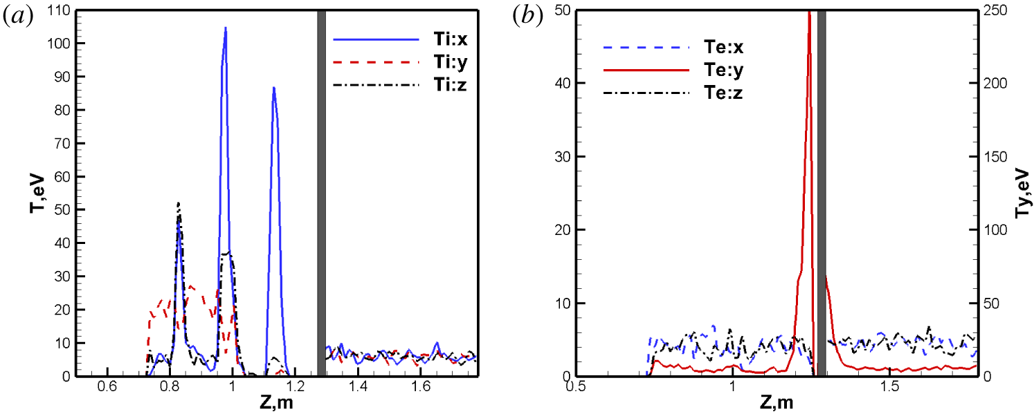
The average temperature differences in figure 21(b) shall be further investigated. Figure 22(a,b) shows the detailed temperature components for each species, and they can effectively explain the $T_{e}$ spikes in figure 21(b). Ions are heated mostly along the $\text{X}-$ direction due to the groups of impinging ions shown in figure 19(a). The major contribution to the average ion temperature $T_{i}$ is from $T_{ix}$, due to the relatively large velocity differences along the $\text{X}-$ direction. For electrons, the temperature component $T_{ey}$ provides the largest contribution, approximately 250 eV, to the average electron temperature. Our simulation results are consistent with the results obtained by Heinrich & Cooke (Reference Heinrich and Cooke2013), and they offered good explanations for these phenomena with the Parker–Murphy theory. Essentially in the wake region, there are two groups of electrons travelling along the magnetic field lines. One group of electrons are bounced back from the symmetric plane and move away from the plane along the $\text{Y}+$ direction; while the other group of electrons moves towards the symmetric plane along the $\text{Y}-$ direction. There are two big spikes in the local $V_{y}$ velocity distribution function, and the velocity deviations from the averaged velocity are much larger, or the local $T_{y}$ is much larger than the other two components.

Figure 22.

Case IV: species temperature component profiles along the $P^{\ast }$ line: (a) ions, (b) electrons.

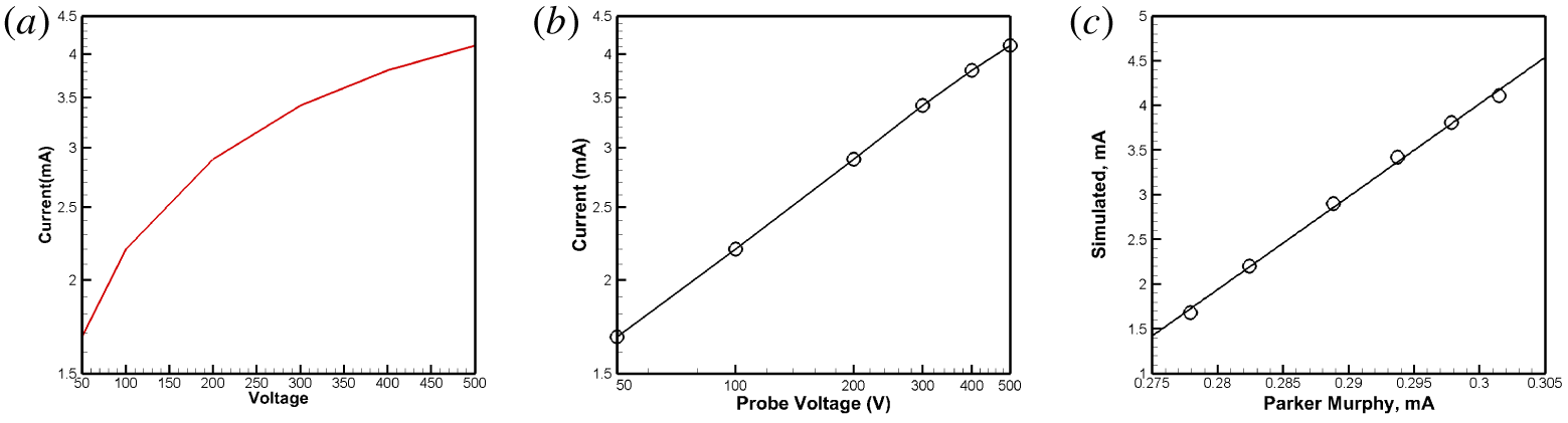
In this work, numerical tests are performed by using different positive probe potential values, and a current–voltage (I–V) curve is obtained for this flow regime. Figure 23(a) presents the final I–V curves in semi-log scales. When plotted in log–log scales, the curve shows a linear relation, as seen in figure 23(b). A linear curving-fitting formula can be obtained as: $I=10^{-0.44}\unicode[STIX]{x1D719}^{0.392}~\text{mA}$. One interesting result is obtained by examining the simulated currents with those values predicted by the Parker–Murphy theory. For drifting plasma flows, usually the measured or simulated currents can be several times larger than the theoretically predicted values. One example is the magnetic limited electron currents collected by the tethering cable during the TSS-1R experiment in space (Janeski, Scales & Hall Reference Janeski, Scales and Hall2014; Cooke & Katz Reference Cooke and Katz1998; Cai Reference Cai2017). In figure 23(c), the Y-axis represents the simulation results, and the $\text{X}$-axis represents the theoretical values predicted by the Parker–Murphy theory. A linear relation can be obtained and shown as figure 23(c), and the curve-fitting expression is: $I_{\text{sim}}=103.85I_{\text{pm}}-27.14~\text{mA}$. It should be mentioned that those coefficients are obtained numerically. With this PIC simulation package, it is feasible to numerically study the current augment ratio. The work described in this paper provides an alternative but more accurate option than various past theoretical predictions.

Figure 23.

Case IV: I–V curve from simulations with a probe potential ranging from 50 to 500 V. (a) In semi-log scales; (b) in log–log scales; (c) simulated currents versus those from the Parker–Murphy theory.