1 Introduction
Rotating Rayleigh–Bénard convection (RBC), i.e. a rotating horizontal fluid layer heated from below and cooled from above, provides a canonical framework for the study of fluid phenomena influenced by rotation and thermal forcing. It has proven to be an indispensable framework for understanding fluid motions in geophysical and astrophysical systems, including planetary atmospheres and interiors (Aurnou et al. Reference Aurnou, Calkins, Cheng, Julien, King, Nieves, Soderlund and Stellmach2015), rapidly rotating stars (Miesch Reference Miesch2005) and open ocean deep convection (Marshall & Schott Reference Marshall and Schott1999). In many of these examples, the dominant influence of rotation results in geostrophy, where the Coriolis force is balanced by the pressure gradient force. Small departures from this dominant force balance, referred to as quasi-geostrophy, are known to be capable of producing turbulent fluid motions characterized by anisotropic eddies elongated along the rotation axis (Sakai Reference Sakai1997). The effect of spatial anisotropy on fluid mixing and global transport properties such as heat and energy transport remains an important and largely unanswered question.
In the context of the Boussinesq approximation for incompressible motions, the rotating RBC problem is completely specified via three non-dimensional parameters, namely the Rayleigh number
 $Ra$
, the Ekman number
 $E$
and the Prandtl number
 ${\it\sigma}$
, defined by
 $$\begin{eqnarray}\displaystyle Ra=\frac{g{\it\alpha}{\rm\Delta}TH^{3}}{{\it\nu}{\it\kappa}},\quad E=\frac{{\it\nu}}{2{\it\Omega}H^{2}},\quad {\it\sigma}=\frac{{\it\nu}}{{\it\kappa}}. & & \displaystyle\end{eqnarray}$$
Here,
 $H$
is the layer depth,
 ${\rm\Delta}T>0$
is the destabilizing temperature difference,
 ${\it\Omega}$
is the rotation rate of the system,
 ${\it\nu}$
is the kinematic viscosity,
 ${\it\kappa}$
is the thermal diffusivity,
 $g$
is the gravitational acceleration and
 ${\it\alpha}$
is the coefficient of thermal expansion. The Rayleigh number measures the magnitude of the thermal forcing and the Ekman number measures the importance of viscous forces relative to the Coriolis force. The Prandtl number is the ratio of the thermal and viscous diffusion time scales in the system and describes the thermophysical properties of the working fluid. Another dimensionless parameter of importance is the convective Rossby number
 $Ro_{cv}=\sqrt{Ra/{\it\sigma}}E$
, which measures the relative importance of thermal forcing and the Coriolis force. Specifically, rotationally constrained convection is characterized by
 $(E,Ro_{cv})\ll 1$
. Importantly, it is known that rotation imparts rigidity to the fluid in the RBC problem which delays the onset of convection until a critical Rayleigh number
 $Ra_{c}\sim E^{-4/3}$
(Chandrasekhar Reference Chandrasekhar1961) is reached with associated
 $Ro_{cv}\sim E^{1/3}$
. At onset, motions are columnar with a horizontal scale
 $L\sim E^{1/3}H$
. By definition of the convective Rossby number, the rotationally constrained branch is defined as
 $E^{1/3}\lesssim Ro_{cv}\ll 1$
and characterized by
 $E^{-4/3}\lesssim Ra\ll E^{-5/3}$
, or, equivalently,
 $1\leqslant \widetilde{Ra}\ll E^{-1/3}$
, where
 $\widetilde{Ra}=RaE^{4/3}$
is the reduced Rayleigh number (Julien et al.
Reference Julien, Knobloch, Rubio and Vasil2012a
). The range of permissible
 $\widetilde{Ra}$
can thus be vast, covering as much as five decades in geophysical and astrophysical settings where
 $E\lesssim 10^{-15}$
. Rich dynamics is observed along this rotationally constrained branch, ranging from coherent laminar to highly turbulent states (Sprague et al.
Reference Sprague, Julien, Knobloch and Werne2006; Julien et al.
Reference Julien, Rubio, Grooms and Knobloch2012b
; Rubio et al.
Reference Rubio, Julien, Knobloch and Weiss2014).
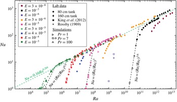
Laboratory (
 ${\it\sigma}\approx 7$
) and DNS (
 ${\it\sigma}=7$
) rotating convection heat transfer data (adapted from Rossby (Reference Rossby1969), King, Stellmach & Aurnou (Reference King, Stellmach and Aurnou2012) and Cheng et al. (Reference Cheng, Stellmach, Ribeiro, Grannan, King and Aurnou2015)). The best-fitting heat transfer trend of
 $Nu\propto (Ra/Ra_{c})^{3.6}$
is plotted for
 $E=10^{-7}$
. For comparison,
 $Nu\propto (Ra/Ra_{c})^{3}$
(King et al.
Reference King, Stellmach and Aurnou2012) is plotted for
 $E=10^{-5}$
and
 $Nu\propto (Ra/Ra_{c})^{6/5}$
(King et al.
Reference King, Stellmach, Noir, Hansen and Aurnou2009, Reference King, Soderlund, Christensen, Wicht and Aurnou2010) for
 $E=10^{-3}$
. It should be noted that with each study at lower
 $E$
, the scaling exponent becomes larger. This implies that the behaviour of rotating convection has not reached an asymptotic regime in the currently accessible range of
 $Nu$
,
 $Ra$
and
 $E$
. Adapted from Cheng et al. (Reference Cheng, Stellmach, Ribeiro, Grannan, King and Aurnou2015).

The efficiency of heat transport, as measured by the non-dimensional Nusselt number
 $Nu=qH/{\it\rho}_{0}c_{p}{\it\kappa}{\rm\Delta}T$
, is perhaps the most common result reported in the literature given that the functional dependence
 $Nu=f(Ra,E,{\it\sigma})$
is tied to the underlying dynamics. Here,
 $q$
is the heat flux and
 ${\it\rho}_{0}c_{p}$
is the volumetric heat capacity. Attempts have been made to characterize the rotationally constrained regime by a heat transport scaling law of the form
 $Nu\propto (Ra/Ra_{c})^{{\it\beta}_{rot}}$
with
 ${\it\beta}_{rot}>1$
(Rossby Reference Rossby1969; Liu & Ecke Reference Liu and Ecke1997; King et al.
Reference King, Stellmach, Noir, Hansen and Aurnou2009; Ecke & Niemela Reference Ecke and Niemela2014). At fixed
 $E\ll 1$
, combined investigations of laboratory experiments and direct numerical simulations (DNS) with no-slip boundaries have reported
 ${\it\beta}_{rot}^{NS}$
values in the range
 $6/5<{\it\beta}_{rot}^{NS}<3.6$
, with a trend towards the upper bound occurring at the lowest Ekman number
 $E=10^{-7}$
(figure 1) (Cheng et al.
Reference Cheng, Stellmach, Ribeiro, Grannan, King and Aurnou2015). At sufficiently large
 $Ra$
, a transition to the weakly rotating or non-rotating regime occurs, characterized by
 $Nu\propto (Ra/Ra_{c})^{{\it\beta}_{norot}}$
, where
 ${\it\beta}_{norot}\in (2/7,1/3)$
(see figure 1). Comparative studies in the presence of stress-free boundaries using DNS have reported similar findings to those seen in figure 1 but with substantially smaller exponents
 ${\it\beta}_{rot}^{SF}\in (3/2,11/5)$
at
 $E=10^{-7}$
(King et al.
Reference King, Stellmach, Noir, Hansen and Aurnou2009; Stellmach et al.
Reference Stellmach, Lischper, Julien, Vasil, Cheng, Ribeiro, King and Aurnou2014). Irrespective of the boundary conditions, King et al. (Reference King, Stellmach, Noir, Hansen and Aurnou2009) have established that the transition to the non-rotating scaling law occurs at smaller and smaller
 $Ro_{cv}$
as the rotation rate increases, i.e.
 $\lim _{E\rightarrow 0}Ro_{cv}^{trans}\sim E^{{\it\gamma}}\rightarrow 0$
, where
 ${\it\gamma}>0$
. This result is attributed to the loss of geostrophic balance in the thermal boundary layer where the local Rossby number reaches unity while the Rossby number in the bulk remains small (Julien et al.
Reference Julien, Knobloch, Rubio and Vasil2012a
).
The difference in the heat transport scaling exponents
 ${\it\beta}_{rot}^{NS}$
and
 ${\it\beta}_{rot}^{SF}$
has been associated with Ekman pumping (Stellmach et al.
Reference Stellmach, Lischper, Julien, Vasil, Cheng, Ribeiro, King and Aurnou2014) – the vertical momentum transport that results from the transition from an interior geostrophic balance to a dominant boundary layer force balance between the Coriolis and viscous forces in the presence of no-slip boundaries. In the linear regime, Ekman pumping promotes the destabilization of the fluid layer, an effect quantified by the positive difference
 $Ra_{SF}-Ra_{NS}=\mathit{O}(E^{1/6})$
in the critical Rayleigh numbers (Niiler & Bisshopp Reference Niiler and Bisshopp1965; Heard & Veronis Reference Heard and Veronis1971). This difference is asymptotically small in the limit
 $E\rightarrow 0$
, indicating that differing mechanical boundaries become asymptotically indistinguishable. By contrast, laboratory experiments and supporting DNS indicate that the discrepancy due to pumping in the fully nonlinear regime appears to remain finite as
 $E\rightarrow 0$
(Stellmach et al.
Reference Stellmach, Lischper, Julien, Vasil, Cheng, Ribeiro, King and Aurnou2014; Cheng et al.
Reference Cheng, Stellmach, Ribeiro, Grannan, King and Aurnou2015). Unfortunately, survey of the high-
 $Ra$
–low-
 $(Ro_{cv},E)$
regime remains a prohibitive challenge for both laboratory experiments and DNS. Laboratory experiments are constrained by their inability to access the rotationally constrained branch at sufficiently low
 $(Ro_{cv},E)$
owing to the decreasing accuracy of global heat transport measurements resulting from unknown heat leaks (King et al.
Reference King, Stellmach, Noir, Hansen and Aurnou2009; Ecke & Niemela Reference Ecke and Niemela2014). Direct numerical simulation studies are restricted by spatiotemporal resolution constraints imposed by the presence of
 $\mathit{O}(E^{1/2}H)$
Ekman boundary layers and fast inertial waves propagating on an
 $\mathit{O}({\it\Omega}^{-1})$
time scale (Nieves, Rubio & Julien Reference Nieves, Rubio and Julien2014; Stellmach et al.
Reference Stellmach, Lischper, Julien, Vasil, Cheng, Ribeiro, King and Aurnou2014).
Although an impediment to DNS, the stiff character of the governing fluid equations in the limit
 $(Ro_{cv},E)\rightarrow 0$
provides a possible path forward for simplifying, or reducing, the governing equations. Indeed, a system of reduced non-hydrostatic quasi-geostrophic equations (NH-QGEs) appropriate for rotating RBC in the presence of stress-free boundaries has been successfully derived and utilized by Julien and collaborators (Julien, Knobloch & Werne Reference Julien, Knobloch and Werne1998; Julien et al.
Reference Julien, Knobloch, Milliff and Werne2006; Sprague et al.
Reference Sprague, Julien, Knobloch and Werne2006; Julien & Knobloch Reference Julien and Knobloch2007; Grooms et al.
Reference Grooms, Julien, Weiss and Knobloch2010; Julien et al.
Reference Julien, Knobloch, Rubio and Vasil2012a
,Reference Julien, Rubio, Grooms and Knobloch
b
; Nieves et al.
Reference Nieves, Rubio and Julien2014; Rubio et al.
Reference Rubio, Julien, Knobloch and Weiss2014). The NH-QGEs, which filter fast inertial waves while retaining inertial waves propagating on slow advective time scales, enable parameter space explorations in the high-
 $Ra$
–low-
 $Ro_{cv}$
limit. The NH-QGEs have been used to identify various flow regimes and heat transfer scaling behaviour as a function of
 $Ra$
, thus providing a valuable roadmap for both DNS and laboratory experiments. Importantly, comparisons with DNS for stress-free boundaries (Stellmach et al.
Reference Stellmach, Lischper, Julien, Vasil, Cheng, Ribeiro, King and Aurnou2014) have established good quantitative agreement in both heat transport and flow morphology at
 $E=10^{-7}$
. For
 $E\ll 10^{-7}$
and large
 $Ra$
, this approach has established an ultimate exponent
 ${\it\beta}_{rot}^{SF}=3/2$
, a result that corresponds to a dissipation-free scaling law in the rotationally constrained turbulence regime (Julien et al.
Reference Julien, Knobloch, Rubio and Vasil2012a
,Reference Julien, Rubio, Grooms and Knobloch
b
).
In the present work, we extend the asymptotic theory resulting in the NH-QGEs to the case of no-slip boundary conditions in which Ekman boundary layers are present. This is the situation pertinent to the laboratory and of relevance to geophysical scenarios such as convection in the Earth’s liquid iron outer core, which is bounded from below by the solid iron inner core and above by a rocky mantle. In agreement with the linear investigation of Heard & Veronis (Reference Heard and Veronis1971), our nonlinear analysis shows that the presence of no-slip boundaries requires the existence of three distinct layers, each characterized by a different dominant physical balance, and hereafter denoted as the outer
 $(o)$
, middle
 $(m)$
and inner
 $(i)$
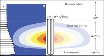
regions (see figure 2).
A schematic diagram of the boundary layer structure for the enhanced-thermal-transport regime of rapidly rotating convection. Three distinct layers characterize the dynamics. The outer layer (o) is geostrophically balanced with dynamically significant flows and thermal perturbations. The middle layer (m) contains the largest thermal perturbations,
 ${\it\theta}$
, of the entire system. The horizontal flow,
 $\boldsymbol{u}_{\bot }$
, responds with a thermal wind driven shear. The inner layer (i) produces a frictional response that causes the flow to vanish at the physical bottom boundary. This layer contains no significant thermal perturbations. The Ekman response produces a vertical momentum flux out of the inner and middle layers and into the bulk fluid. The details of the dynamical pathway ensure that the Ekman flux correlates with the largest bulk vertical flows, thermal anomalies and vorticity. This correlation is the means by which no-slip boundary layers can so significantly enhance the heat flux through the entire system.

The outer region
 $(o)$
corresponds to the fluid interior (i.e. the bulk region of depth
 $\mathit{O}(H)$
). Within this region, fluid motions are horizontally non-divergent and in pointwise geostrophic balance. The dynamics is asymptotically described by the NH-QGEs investigated by Julien and collaborators (Reference Julien, Knobloch and Werne1998, Reference Julien, Knobloch, Milliff and Werne2006, Reference Julien and Knobloch2007, Reference Julien, Knobloch, Rubio and Vasil2012a
, Reference Julien, Rubio, Grooms and Knobloch2012b
, Reference Ecke and Niemela2014). As in the classical quasi-geostrophic equations (Charney Reference Charney1948, Reference Charney1971; Eady Reference Eady1949; Pedlosky Reference Pedlosky1987; Vallis Reference Vallis2006), toroidal or vortical fluid motions aligned with the axis of rotation are forced solely by the vortex stretching associated with the linear Coriolis force. The NH-QGEs differ from the classical quasi-geostrophic equations in that vertical motions required by vortex stretching are now comparable in magnitude to horizontal motions, and thus the non-hydrostatic inertial acceleration force must be retained in the vertical momentum balance. This results in a dynamic, as opposed to a diagnostic, evolution of the vertical velocity field. In the presence of stress-free boundaries, the NH-QGEs are sufficient to completely describe all of the ‘slow’ dynamics occurring within the fluid layer.
The inner
 $(i)$
regions are the
 $\mathit{O}(E^{1/2}H)$
Ekman boundary layers immediately adjacent to the horizontal boundaries. These layers are required to attenuate the interior geostrophic velocity fields to zero. Within them, the geostrophic balance of the interior is relaxed, and as a consequence fluid motions become horizontally divergent with cross-isobaric flow. Mass conservation requires that vertical motions are induced, a process referred to as Ekman pumping. The dynamics within the Ekman layers is described by a classical set of reduced linear equations (Greenspan Reference Greenspan1969), where as a consequence of the
 $L/H=\mathit{O}(E^{1/3})$
spatial anisotropy and the vortical magnitude
 ${\it\zeta}^{\ast }$
observed in rotating RBC (Chandrasekhar Reference Chandrasekhar1961), vertical pumping velocities of magnitude
 $w_{E}^{\ast }=\mathit{O}(E^{1/2}{\it\zeta}^{\ast }H)=\mathit{O}(E^{1/6}{\it\zeta}^{\ast }L)$
are found (Niiler & Bisshopp Reference Niiler and Bisshopp1965; Heard & Veronis Reference Heard and Veronis1971). As done in large-scale oceanic and atmospheric applications, this linear property of the dynamics can be successfully utilized, and the effects of this layer on the fluid interior can be parameterized by the application of simple pumping boundary conditions (Pedlosky Reference Pedlosky1987). This parameterized approach has been applied successfully in numerous previous works, including the investigation of Stewartson layer instabilities (Schaeffer & Cardin Reference Schaeffer and Cardin2005), spherical convection (Aubert, Gillet & Cardin Reference Aubert, Gillet and Cardin2003; Calkins et al.
Reference Calkins, Aurnou, Eldredge and Julien2012) and rotating RBC (Stellmach et al.
Reference Stellmach, Lischper, Julien, Vasil, Cheng, Ribeiro, King and Aurnou2014), and is also employed in the present work.
As shown by Heard & Veronis (Reference Heard and Veronis1971), Ekman pumping induces thermal fluctuations that cannot be regulated within the Ekman boundary layer to satisfy the thermal boundary conditions. Middle layers
 $(m)$
of depth
 $\mathit{O}(E^{1/3}H)$
arise that separate the Ekman boundary layers from the geostrophically balanced fluid interior. Importantly, the requirement that thermal fluctuations vanish at the fixed-temperature bounding plates necessitates the introduction of vertical diffusion for temperature fluctuations. This is an insignificant process in the interior in the rapidly rotating limit (Sprague et al.
Reference Sprague, Julien, Knobloch and Werne2006; Julien et al.
Reference Julien, Knobloch, Rubio and Vasil2012a
). However, as shown in this paper, the middle region is characterized by a thermal wind balance, i.e. a geostrophic and hydrostatic diagnostic balance, and the dynamics of this region evolves according to an advection–diffusion equation for the temperature fluctuations forced by Ekman pumping. Specifically, the magnitude of the vertical advection of the mean temperature field within the middle layers increases with the Rayleigh number until it becomes a dominant source of buoyancy production that is comparable to that produced in the geostrophic interior. This enhancement is due to the intensification of vortical motions, and hence vertical transport, in the vicinity of the boundaries. Convective fluxes driven by Ekman transport are also comparable to that produced in the geostrophic interior. Therefore,
 $\mathit{O}(1)$
changes to the heat transport are to be expected, as observed in laboratory experiments and simulations (Stellmach et al.
Reference Stellmach, Lischper, Julien, Vasil, Cheng, Ribeiro, King and Aurnou2014; Cheng et al.
Reference Cheng, Stellmach, Ribeiro, Grannan, King and Aurnou2015).
We show that the asymptotic results for the different regions may be combined into a single composite system of reduced equations, which we refer to as the CNH-QGEs (composite non-hydrostatic quasi-geostrophic equations). On the rotationally constrained branch of RBC, the CNH-QGEs are valid in the interval
 $\mathit{O}(1)\lesssim \widetilde{Ra}\lesssim \mathit{O}(E^{-1/3})$
. The linear stability properties of these equations are shown to be consistent with earlier work (Niiler & Bisshopp Reference Niiler and Bisshopp1965; Heard & Veronis Reference Heard and Veronis1971). Moreover, comparisons with the NH-QGEs for single-mode (or single-horizontal-wavenumber) solutions show that significant departures in heat transport occur in the interval
 $\mathit{O}(E^{-1/9})\lesssim \widetilde{Ra}\lesssim \mathit{O}(E^{-1/3})$
.
The remainder of this paper is organized as follows. In § 2, we present the formulation of the rotating RBC problem in terms of the incompressible Navier–Stokes equations. In § 3, we present the asymptotic development in the presence of no-slip bounding plates using the ‘method of composite expansions’ (see Nayfeh (Reference Nayfeh2008, § 4.2)). In particular, the Ekman and thermal wind boundary layers are identified and analysed. The significance of Ekman pumping is also deduced by determining the Rayleigh number threshold at which the resulting vertical pumping velocity induces order-one changes in the heat transport. It is also established that such a transition always occurs on the rotationally constrained branch of RBC. In § 4, we present the composite reduced model, i.e. the CNH-QGEs, where the dynamics of each layer are combined into a unified description (see (4.13a )–(4.15)). Results from the model are presented in § 5, and establish that this unified model captures the physics associated with no-slip boundary conditions observed in laboratory experiments and DNS. Concluding remarks are given in § 6.
2 Governing equations
We consider thermally driven fluid flows that are characterized by the dimensional scales of length
 $[L]$
, velocity
 $[U]$
, time
 $[L/U]$
, pressure
 $[P]$
and destabilizing temperature jump
 $[{\rm\Delta}T]$
. Assuming a Cartesian coordinate system
 $\boldsymbol{x}=(x,y,z),$
we adopt the Rayleigh–Bénard configuration of a plane-parallel geometry rotating about the
 $z$
-axis with constant angular velocity
 ${\it\Omega}$
in the presence of constant gravity
 $\boldsymbol{g}=-g\hat{\boldsymbol{z}}$
. The non-dimensional equations of motion are given by the Boussinesq equations
 $$\begin{eqnarray}\displaystyle & \displaystyle D_{t}\boldsymbol{u}+\frac{1}{Ro}\widehat{\boldsymbol{z}}\times \boldsymbol{u}=-Eu\boldsymbol{{\rm\nabla}}p+{\it\Gamma}{\it\theta}\widehat{\boldsymbol{z}}+\frac{1}{Re}{\rm\nabla}^{2}\boldsymbol{u}, & \displaystyle\end{eqnarray}$$
 $$\begin{eqnarray}\displaystyle & \displaystyle D_{t}{\it\theta}=\frac{1}{Pe}{\rm\nabla}^{2}{\it\theta}, & \displaystyle\end{eqnarray}$$
 $$\begin{eqnarray}\displaystyle & \displaystyle \boldsymbol{{\rm\nabla}}\boldsymbol{\cdot }\boldsymbol{u}=0 & \displaystyle\end{eqnarray}$$
for the velocity field
 $\boldsymbol{u}\equiv (u,v,w)$
, temperature
 ${\it\theta}$
and pressure
 $p$
, where the material derivative
 $D_{t}\equiv \partial _{t}+\boldsymbol{u}\boldsymbol{\cdot }\boldsymbol{{\rm\nabla}}$
. The non-dimensional parameters that appear are defined as
 $$\begin{eqnarray}Ro=\frac{U}{2{\it\Omega}L},\quad Eu=\frac{P}{{\it\rho}_{o}U^{2}},\quad {\it\Gamma}=\frac{g{\it\alpha}{\rm\Delta}TL}{U^{2}},\quad Re=\frac{UL}{{\it\nu}},\quad Pe=\frac{UL}{{\it\kappa}},\end{eqnarray}$$
respectively denoting the Rossby, Euler, buoyancy, Reynolds and Péclet numbers. In the present work, we are interested in the rotationally constrained regime characterized by
 $Ro\ll 1$
and aspect ratio
 $A\equiv H/L=Ro^{-1}\gg 1$
for columnar structures of depth
 $H$
(Julien et al.
Reference Julien, Knobloch and Werne1998, Reference Julien, Knobloch, Milliff and Werne2006; Sprague et al.
Reference Sprague, Julien, Knobloch and Werne2006; Julien et al.
Reference Julien, Rubio, Grooms and Knobloch2012b
).
For fluid motions in a statistically stationary state, the non-dimensional vertical heat transport, i.e. the Nusselt number
 $Nu$
, is given by
 $$\begin{eqnarray}Nu=\frac{H}{L}\left(-\partial _{z}\overline{{\it\theta}}^{\mathscr{A,T}}+Pe\;\overline{w{\it\theta}}^{\mathscr{A,T}}\right),\end{eqnarray}$$
obtained upon averaging equation (2.2) over time
 $\mathscr{T}$
and the horizontal
 $(x,y)$
cross-section. Here,
 $\overline{f}^{\mathscr{A,T}}=\lim _{\mathscr{T}\rightarrow \infty }(1/\mathscr{AT})\int _{\mathscr{A,T}}f\,\text{d}x\,\text{d}y\,\text{d}t$
, where
 $\mathscr{A}$
is the horizontal cross-sectional area. This result indicates that the heat flux
 $Nu$
through the layer is constant at every vertical level.
3 Asymptotic development
It is well established that in the geophysically and astrophysically relevant regimes
 $Ro\ll 1$
the presence of fast inertial waves, propagating on
 $\mathit{O}(Ro^{-1})$
time scales, poses a severe restriction on DNS. This is because the discretized equations resulting from the Boussinesq equations will, in general, be coupled through the Coriolis force
 $Ro^{-1}\widehat{\boldsymbol{z}}\times \boldsymbol{u}$
. This coupling is routinely eliminated by an explicit treatment in many time-stepping algorithms, i.e. by its relegation and evaluation at previous steps. This favourable numerical situation occurs at the expense of imposing severe time-stepping restrictions. Implicit treatment circumvents this issue. However, prohibitive time-stepping restrictions persist due to the Ekman-dependent Courant–Friedrichs–Lewy (CFL) time constraint associated with advective nonlinearities. The evolution of turbulent eddies is insensitive to fast inertial waves which can be filtered from the governing equations by asymptotic reduction methods in much the same manner as done in atmospheric and oceanic sciences for stably stratified layers. Indeed, Julien and collaborators (Julien et al.
Reference Julien, Knobloch, Milliff and Werne2006; Sprague et al.
Reference Sprague, Julien, Knobloch and Werne2006; Julien & Knobloch Reference Julien and Knobloch2007) have established that an asymptotic reduction of the governing equations (2.1)–(2.3) can be deduced upon using
 $Ro\equiv {\it\epsilon}$
as a small parameter and introducing the distinguished limit
 $$\begin{eqnarray}A={\it\epsilon}^{-1},\quad Eu={\it\epsilon}^{-2},\quad {\it\Gamma}=\mathit{O}({\it\epsilon}^{-1}),\quad Re=Pe=\mathit{O}(1).\end{eqnarray}$$
For the appropriate choice of the horizontal diffusive velocity scale,
 $U={\it\nu}/L$
, it follows that
 $$\begin{eqnarray}E={\it\epsilon}^{3},\quad {\it\Gamma}=\frac{Ra}{{\it\sigma}}{\it\epsilon}^{3},\quad Re=1,\quad Pe={\it\sigma},\end{eqnarray}$$
such that
 ${\it\Gamma}=\widetilde{{\it\Gamma}}{\it\epsilon}^{-1}$
. Here,
 ${\it\sigma}\widetilde{{\it\Gamma}}=Ra{\it\epsilon}^{4}=\mathit{O}(1)$
corresponds to the reduced Rayleigh number
 $\widetilde{Ra}={\it\sigma}\widetilde{{\it\Gamma}}$
involving the Prandtl number
 ${\it\sigma}$
.
In accord with figure 2, we anticipate the existence of three distinct layers: the bulk and middle regions, and the Ekman layers, each with their respective non-dimensional depths
 $\mathit{O}({\it\epsilon}^{-1}),\mathit{O}(1)$
and
 $\mathit{O}({\it\epsilon}^{1/2})$
. We therefore employ a multiple-scale expansion in the vertical direction and time,
 $$\begin{eqnarray}\partial _{z}\rightarrow {\it\epsilon}^{-1/2}\partial _{{\it\mu}}+\partial _{z}+{\it\epsilon}\partial _{Z},\quad \partial _{t}\rightarrow \partial _{t}+{\it\epsilon}^{2}\partial _{{\it\tau}},\end{eqnarray}$$
where the slow vertical coordinate in the bulk is defined by
 $Z={\it\epsilon}z$
, the fast coordinate of the Ekman layer is defined by
 ${\it\mu}={\it\epsilon}^{-1/2}z$
and the slow time is defined by
 ${\it\tau}={\it\epsilon}^{2}t$
. We find that this set-up necessitates the decomposition of the fluid variables into mean (horizontally averaged) and fluctuating (horizontally varying) components, respectively denoted by overbars and primes, e.g.
 $$\begin{eqnarray}\boldsymbol{u}=\overline{\boldsymbol{u}}+\boldsymbol{u}^{\prime },\quad \overline{\boldsymbol{u}}=\frac{1}{\mathscr{A}}\int _{\mathscr{A}}\boldsymbol{u}\,\text{d}x\,\text{d}y,\quad \overline{\boldsymbol{u}^{\prime }}=0.\end{eqnarray}$$
Averaging over the fast time
 $t$
is also required,
 $$\begin{eqnarray}\overline{\boldsymbol{u}}^{\mathscr{T}}=\lim _{\mathscr{ T}\rightarrow \infty }\frac{1}{\mathscr{T}}\int _{\mathscr{T}}\boldsymbol{u}\,\text{d}t.\end{eqnarray}$$
We note a posteriori that, unlike derivations of the reduced dynamics in the presence of stress-free boundaries (Sprague et al. Reference Sprague, Julien, Knobloch and Werne2006), the consideration of no-slip boundaries and Ekman layers requires the separation of spatial and time-averaging operations as performed here.
To proceed, all fluid variables are decomposed into outer
 $(o)$
, middle
 $(m,\pm )$
and inner
 $(i,\pm )$
components representing the fluid bulk, middle regions and Ekman layers. For example,
 $$\begin{eqnarray}\displaystyle \boldsymbol{u} & = & \displaystyle \boldsymbol{U}^{(o)}(x,y,Z,t,{\it\tau})+\boldsymbol{U}^{(m,-)}(x,y,z,t,{\it\tau})+\boldsymbol{U}^{(m,+)}(x,y,z,t,{\it\tau})\nonumber\\ \displaystyle & & \displaystyle +\,\boldsymbol{U}^{(i,-)}(x,y,{\it\mu},t,{\it\tau})+\boldsymbol{U}^{(i,+)}(x,y,{\it\mu},t,{\it\tau}).\end{eqnarray}$$
Here, capitalizations are used to identify the individual contributions of the fluid variables to each region, and the notation
 $\pm$
denotes the upper and lower boundaries respectively. The boundary layer coordinates
 ${\it\mu},z$
are assumed to increase away from the physical boundaries at
 $Z=0,1.$
Each region of the fluid layer may be accessed by the following actions for the outer, middle and inner limits:
 $$\begin{eqnarray}\displaystyle \lim (\boldsymbol{u})^{o} & \equiv & \displaystyle \lim _{{{\it\mu}\rightarrow \infty \atop z\rightarrow \infty }}(\boldsymbol{u})=\boldsymbol{U}^{(o)}\nonumber\\ \displaystyle & \Rightarrow & \displaystyle \lim (\boldsymbol{U}^{(o)})^{o}=\boldsymbol{U}^{(o)},~\lim (\boldsymbol{U}^{(m)},\boldsymbol{U}^{(i)})^{o}=0,\end{eqnarray}$$
 $$\begin{eqnarray}\displaystyle \lim (\boldsymbol{u})^{m} & \equiv & \displaystyle \lim _{{{\it\mu}\rightarrow \infty \atop Z\rightarrow 0}}(\boldsymbol{u})=\boldsymbol{U}^{(o)}(0)+\boldsymbol{U}^{(m)}\nonumber\\ \displaystyle & \Rightarrow & \displaystyle \lim (\boldsymbol{U}^{(o)})^{m}=\boldsymbol{U}^{(o)}(0),~\lim (\boldsymbol{U}^{(m)})^{m}=\boldsymbol{U}^{(m)},~\lim (\boldsymbol{U}^{(i)})^{m}=0,\end{eqnarray}$$
 $$\begin{eqnarray}\displaystyle \lim (\boldsymbol{u})^{i} & \equiv & \displaystyle \lim _{{z\rightarrow 0\atop Z\rightarrow 0}}(\boldsymbol{u})=\boldsymbol{U}^{(o)}(0)+\boldsymbol{U}^{(m)}(0)+\boldsymbol{U}^{(i)}\nonumber\\ \displaystyle & \Rightarrow & \displaystyle \lim (\boldsymbol{U}^{(o)}+\boldsymbol{U}^{(m)})^{i}=\boldsymbol{U}^{(o)}(0)+\boldsymbol{U}^{(m)}(0),\lim (\boldsymbol{U}^{(i)})^{i}=\boldsymbol{U}^{(i)}.\end{eqnarray}$$
Similar expressions hold for the upper inner and middle layers located at
 $Z=1$
upon replacing
 $(0)$
with
 $(1)$
. By definition, the middle variables are identically zero in the outer region, while the inner variables are identically zero in both the middle and outer regions. Contributions to regions
 $(i)$
or
 $(m)$
involving outer variables, indicated in (3.8) and (3.9), are obtained by Taylor-expanding and then taking the appropriate limit. Hereafter, for notational convenience, contractions
 $(m,\pm )\rightarrow (m)$
and
 $(i,\pm )\rightarrow (i)$
are used when referring to both upper and lower regions. Furthermore, contractions such as
 $(0)$
omit reference to the dependence on other variables (i.e.
 $x,y,t,{\it\tau}$
) and refer to the vertical coordinate.
Asymptotic series in powers of
 ${\it\epsilon}$
are now introduced for all fluid variables and substituted into the governing equations (2.1)–(2.3). An order by order analysis is then performed. The asymptotic procedure using decompositions of the form (3.6) with (3.7)–(3.9) is referred to as the ‘method of composite expansions’ (see Nayfeh (Reference Nayfeh2008, § 4.2)). Specifically, rather than using the ‘method of matched asymptotic expansions’, i.e. first determining the inner and outer expansions analytically, matching them, and then forming the composite expansion (Van Dyke Reference Van Dyke1975), here variables of the form (3.6) are automatically valid everywhere provided that they satisfy the physical boundary conditions at the bounding plates.
3.1 The outer region: NH-QGEs
Within the fluid interior, inner
 $(i)$
and middle
 $(m)$
variables are identically zero. We introduce expansions in powers of
 ${\it\epsilon}$
of the form
 $$\begin{eqnarray}\displaystyle \boldsymbol{u}^{(o)}=\lim (\boldsymbol{u})^{o}=\boldsymbol{U}_{0}^{(o)}+{\it\epsilon}\boldsymbol{U}_{1}^{(o)}+{\it\epsilon}^{2}\boldsymbol{U}_{2}^{(o)}+\cdots \,, & & \displaystyle\end{eqnarray}$$
where
 $Ro\equiv {\it\epsilon}$
(Julien et al.
Reference Julien, Knobloch, Milliff and Werne2006; Sprague et al.
Reference Sprague, Julien, Knobloch and Werne2006; Julien & Knobloch Reference Julien and Knobloch2007). The leading-order mean component satisfies the motionless hydrostatic balance
 $$\begin{eqnarray}\displaystyle \overline{\boldsymbol{U}}_{0}^{(o)}=0,\quad \partial _{Z}\overline{P}_{0}^{(o)}=\frac{\widetilde{Ra}}{{\it\sigma}}\overline{{\it\Theta}}_{0}^{(o)}, & & \displaystyle\end{eqnarray}$$
together with
 $P_{0}^{\prime (o)}={\it\Theta}_{0}^{\prime (o)}=0$
. The leading-order convective dynamics is found to be incompressible and geostrophically balanced, i.e.
 $$\begin{eqnarray}\displaystyle \left.\begin{array}{@{}c@{}}\widehat{\boldsymbol{z}}\times \boldsymbol{U}_{0}^{\prime (o)}+\boldsymbol{{\rm\nabla}}P_{1}^{\prime (o)}=0,\\ \boldsymbol{{\rm\nabla}}\boldsymbol{\cdot }\boldsymbol{U}_{0}^{\prime (o)}=0,\end{array}\quad \text{or}\quad \mathscr{L}_{geo}\left(\begin{array}{@{}c@{}}\boldsymbol{U}_{0}^{\prime (o)}\\ P_{1}^{\prime (o)}\end{array}\right)=\mathbf{0},\right\} & & \displaystyle\end{eqnarray}$$
where
 $\mathscr{L}_{geo}$
denotes the geostrophic operator. By definition, all outer variables are independent of
 $z$
, and so
 $\boldsymbol{{\rm\nabla}}=\boldsymbol{{\rm\nabla}}_{\bot }\equiv (\partial _{x},\partial _{y},0)$
. If the small-scale
 $z$
dependence were retained, geostrophy would automatically imply the Proudman–Taylor (PT) constraint
 $\partial _{z}(\boldsymbol{U}_{0}^{\prime (o)},P_{1}^{\prime (o)})\equiv 0$
on the small vertical scale
 $z$
(Proudman Reference Proudman1916; Taylor Reference Taylor1923). The diagnostic balance given by (3.12) is solved by
 $$\begin{eqnarray}\boldsymbol{U}_{0}^{\prime (o)}=\boldsymbol{{\rm\nabla}}^{\bot }{\it\Psi}_{0}^{(o)}+W_{0}^{(o)}\widehat{\boldsymbol{z}},\quad P_{1}^{\prime (o)}={\it\Psi}_{0}^{(o)},\end{eqnarray}$$
for the streamfunction
 ${\it\Psi}_{0}^{(o)}(x,y,Z,t,{\it\tau})$
and vertical velocity
 $W_{0}^{(o)}(x,y,Z,t,{\it\tau})$
. Here, we adopt the definition
 $\boldsymbol{{\rm\nabla}}^{\bot }{\it\Psi}_{0}^{(o)}\equiv -\boldsymbol{{\rm\nabla}}_{\bot }\times {\it\Psi}_{0}^{(o)}\widehat{\boldsymbol{z}}$
with
 $\boldsymbol{{\rm\nabla}}^{\bot }=(-\partial _{y},\partial _{x},0)$
, so that the pressure is now identified as the geostrophic streamfunction. It follows that leading-order motions are horizontally non-divergent with
 $\boldsymbol{{\rm\nabla}}_{\bot }\boldsymbol{\cdot }\boldsymbol{U}_{0\bot }^{\prime (o)}=0$
. Three-dimensional incompressibility is captured at the next order,
 $\mathit{O}({\it\epsilon})$
, where
 $$\begin{eqnarray}\boldsymbol{{\rm\nabla}}_{\bot }\boldsymbol{\cdot }\boldsymbol{U}_{1\bot }^{\prime (o)}+\partial _{Z}W_{0}^{(o)}=0.\end{eqnarray}$$
This results in the production of subdominant ageostrophic motions
 $\boldsymbol{U}_{1\bot }^{\prime (o)}$
driven by vertical gradients in
 $W_{0}$
. The prognostic evolution of these variables is obtained from balances at next order,
 $$\begin{eqnarray}\displaystyle \mathscr{L}_{geo}\left(\begin{array}{@{}c@{}}\boldsymbol{U}_{1}^{\prime (o)}\\ P_{2}^{\prime (o)}\end{array}\right) & = & \displaystyle \text{RHS}\nonumber\\ \displaystyle & \equiv & \displaystyle \left(\begin{array}{@{}c@{}}-D_{0t}^{\bot }\boldsymbol{U}_{0}^{\prime (o)}-\partial _{Z}P_{1}\widehat{\boldsymbol{z}}+\displaystyle \frac{\widetilde{Ra}}{{\it\sigma}}{\it\Theta}_{1}^{\prime (o)}\widehat{\boldsymbol{z}}+{\rm\nabla}_{\bot }^{2}\boldsymbol{U}_{0}^{\prime (o)}\\ -\partial _{Z}W_{0}\end{array}\right),\end{eqnarray}$$
obtained by projecting RHS onto the null space of
 $\mathscr{L}_{geo}$
(Sprague et al.
Reference Sprague, Julien, Knobloch and Werne2006; Calkins, Julien & Marti Reference Calkins, Julien and Marti2013). This amounts to performing the projections
 $\widehat{\boldsymbol{z}}\boldsymbol{\cdot }$
and
 $\boldsymbol{{\rm\nabla}}^{\bot }\boldsymbol{\cdot }$
on (3.15). On noting that
 $D_{0t}^{\bot }\equiv \partial _{t}+\boldsymbol{U}_{0\bot }^{\prime (o)}\boldsymbol{\cdot }\boldsymbol{{\rm\nabla}}_{\bot }$
, this procedure results in asymptotically reduced equations for the vertical vorticity
 ${\it\zeta}_{0}^{(o)}={\rm\nabla}_{\bot }^{2}{\it\Psi}_{0}^{(o)}$
, vertical velocity
 $W_{0}^{(o)}$
and thermal anomaly
 ${\it\Theta}_{1}^{\prime (o)}$
:
 $$\begin{eqnarray}\displaystyle & \displaystyle D_{0t}^{\bot }{\it\zeta}_{0}^{(o)}-\partial _{Z}W_{0}^{(o)}={\rm\nabla}_{\bot }^{2}{\it\zeta}_{0}^{(o)}, & \displaystyle\end{eqnarray}$$
 $$\begin{eqnarray}\displaystyle & \displaystyle D_{0t}^{\bot }W_{0}^{(o)}+\partial _{Z}{\it\Psi}_{0}^{(o)}=\frac{\widetilde{Ra}}{{\it\sigma}}{\it\Theta}_{1}^{\prime (o)}+{\rm\nabla}_{\bot }^{2}W_{0}^{(o)}, & \displaystyle\end{eqnarray}$$
 $$\begin{eqnarray}\displaystyle & \displaystyle D_{0t}^{\bot }{\it\Theta}_{1}^{\prime (o)}+W_{0}^{(o)}\partial _{Z}\overline{{\it\Theta}}_{0}^{(o)}=\frac{1}{{\it\sigma}}{\rm\nabla}_{\bot }^{2}{\it\Theta}_{1}^{\prime (o)}. & \displaystyle\end{eqnarray}$$
The evolution of the mean temperature field
 $\overline{{\it\Theta}}_{0}^{(o)}$
is deduced at
 $\mathit{O}({\it\epsilon}^{2})$
upon averaging over the fast scales
 $x,y,z,t$
:
 $$\begin{eqnarray}\displaystyle \partial _{{\it\tau}}\overline{{\it\Theta}}_{0}^{(o)}+\partial _{Z}\left(\overline{\overline{W_{0}^{(o)}{\it\Theta}_{1}^{\prime (o)}}}^{\mathscr{T}}\right) & = & \displaystyle \frac{1}{{\it\sigma}}\partial _{ZZ}\overline{{\it\Theta}}_{0}^{(o)}.\end{eqnarray}$$
In a statistically stationary state, it follows that
 $$\begin{eqnarray}Nu={\it\sigma}\left(\overline{\overline{W_{0}^{(o)}{\it\Theta}_{1}^{\prime (o)}}}^{\mathscr{T}}\right)-\partial _{Z}\overline{{\it\Theta}}_{0}^{(o)}.\end{eqnarray}$$
Equations (3.16)–(3.18), (3.11) and (3.19) constitute the asymptotically reduced system referred to as the NH-QGEs. A notable feature in the NH-QGEs is the absence of (higher-order) vertical advection. This is a hallmark characteristic of quasi-geostrophic theory. Equation (3.16) states that vertical vorticity, or toroidal motion, is affected by horizontal advection, vortex stretching arising from the linear Coriolis force and horizontal diffusion, while (3.17) shows that vertical motion is affected by horizontal advection, unbalanced pressure gradient, horizontal diffusion and buoyancy. The buoyancy forces are captured by the fluctuating and mean temperature equations (3.18) and (3.19).
The system (3.16)–(3.19) is accompanied by impenetrable boundary conditions
 $$\begin{eqnarray}W_{0}^{(o)}(0)=W_{0}^{(o)}(1)=0,\end{eqnarray}$$
together with thermal conditions, hereafter taken to be the fixed temperature conditions
 $$\begin{eqnarray}\overline{{\it\Theta}}_{0}^{(o)}(0)=1,\quad \overline{{\it\Theta}}_{0}^{(o)}(1)=0.\end{eqnarray}$$
In the presence of impenetrable boundaries, the boundary limits
 $Z\rightarrow 0$
or
 $Z\rightarrow 1$
of (3.18) for the temperature fluctuations
 ${\it\Theta}_{1}^{(o)}$
reduce to the advection–diffusion equation
 $$\begin{eqnarray}\displaystyle D_{0t}{\it\Theta}_{1}^{\prime (o)}=\frac{1}{{\it\sigma}}{\rm\nabla}_{\bot }^{2}{\it\Theta}_{1}^{\prime (o)}. & & \displaystyle\end{eqnarray}$$
The horizontally averaged variance
 $\overline{{\it\Theta}_{1}^{\prime (o)2}}$
for such an equation evolves according to
 $$\begin{eqnarray}\displaystyle \partial _{t}\overline{{\it\Theta}_{1}^{\prime (o)2}}=-\frac{1}{{\it\sigma}}\overline{|\boldsymbol{{\rm\nabla}}_{\bot }{\it\Theta}_{1}^{\prime (o)}|^{2}}. & & \displaystyle\end{eqnarray}$$
Therefore,
 $\overline{{\it\Theta}_{1}^{\prime (o)2}}$
decreases monotonically to zero in time, implying the implicit thermal boundary condition
 ${\it\Theta}_{1}^{\prime (o)}(0)={\it\Theta}_{1}^{\prime (o)}(1)=0$
. Together with the impenetrability condition (3.21), the vertical momentum equation (3.17) implies that motions along the horizontal boundaries are implicitly stress-free with
 $$\begin{eqnarray}\partial _{Z}{\it\Psi}_{0}^{(o)}(0)=\partial _{Z}{\it\Psi}_{0}^{(o)}(1)=0.\end{eqnarray}$$
If rapidly rotating RBC in the presence of stress-free boundary conditions is the primary objective, a well-posed closed system is obtained from (3.16)–(3.18), (3.11) and (3.19) together with impenetrable boundary conditions (3.21) and fixed mean temperature boundary conditions (3.22).
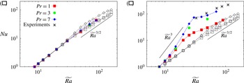
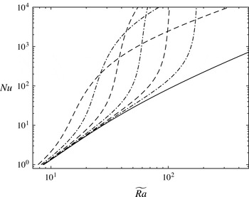
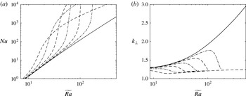
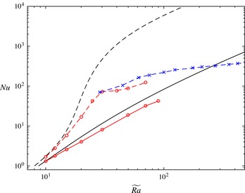
Comparison of the Nusselt number
 $Nu$
as a function of the reduced Rayleigh number
 $\widetilde{Ra}=RaE^{4/3}$
for NH-QGEs and DNS with (a) stress-free and (b) no-slip boundary conditions. The filled symbols illustrate DNS data obtained at
 $E=10^{-7}$
while the open symbols are from the reduced NH-QGEs. Data courtesy of Julien et al. (Reference Julien, Rubio, Grooms and Knobloch2012b
) and Stellmach et al. (Reference Stellmach, Lischper, Julien, Vasil, Cheng, Ribeiro, King and Aurnou2014).

3.1.1 Validity of the NH-QGEs
In the presence of stress-free boundary conditions, the NH-QGEs remain valid throughout the entire flow domain provided that geostrophy, equation (3.12), holds. This remains so provided that the local Rossby number
 $Ro_{l}\ll 1$
. Given
 $\boldsymbol{U}_{0}^{\ast }=\boldsymbol{U}_{0}^{(o)}{\it\nu}/L$
, one finds
 $$\begin{eqnarray}Ro_{l}=\frac{|\boldsymbol{U}_{0}^{\ast }|}{2{\it\Omega}L}=|\boldsymbol{U}_{0}^{(o)}|E\left(\frac{H}{L}\right)^{2}=|\boldsymbol{U}_{0}^{(o)}|E^{1/3}\Rightarrow |\boldsymbol{U}_{0}^{(o)}|\sim |{\it\zeta}_{0}^{(o)}|=o({\it\epsilon}^{-1}).\end{eqnarray}$$
(The Landau notation lower-case
 $o$
denotes a function that is of lower order of magnitude than a given function; that is, the function
 $o({\it\epsilon}^{-1})$
is of a lower order than the function
 ${\it\epsilon}^{-1}$
.) In a detailed investigation of the NH-QGEs, Julien et al. (Reference Julien, Knobloch, Rubio and Vasil2012a
) have shown that this criterion is violated at the transitional value
 $$\begin{eqnarray}\widetilde{Ra}_{tr}=\mathit{O}({\it\epsilon}^{-4/5}),\quad Ro_{tr}=\mathit{O}({\it\epsilon}^{3/5})\quad \text{as }{\it\epsilon}\rightarrow 0.\end{eqnarray}$$
In this regime, the thermal boundary layers experience a loss of geostrophic balance. This provides an upper bound for comparisons of the NH-QGEs with DNS with stress-free boundary conditions. Indeed, as illustrated in figure 3(a) for
 $E=10^{-7}$
, within the regime of validity,
 $\widetilde{Ra}\lesssim 70$
, good quantitative agreement in the heat transport measurements is observed (Stellmach et al.
Reference Stellmach, Lischper, Julien, Vasil, Cheng, Ribeiro, King and Aurnou2014). Simulations (Julien et al.
Reference Julien, Rubio, Grooms and Knobloch2012b
; Nieves et al.
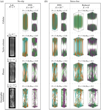
Reference Nieves, Rubio and Julien2014) of the NH-QGEs prior to this transition have revealed four different flow morphologies subsequently confirmed by both DNS (Stellmach et al.
Reference Stellmach, Lischper, Julien, Vasil, Cheng, Ribeiro, King and Aurnou2014) and laboratory experiments (Cheng et al.
Reference Cheng, Stellmach, Ribeiro, Grannan, King and Aurnou2015) as
 $\widetilde{Ra}$
is increased (see figure 4): a cellular regime, a convective Taylor column (CTC) regime consisting of weakly interacting shielded columns, a plume regime where the CTCs have lost stability and finally a geostrophic turbulence regime that is also associated with an inverse energy cascade that produces a depth-independent large-scale dipole vortex pair. All regimes are identifiable by changes in the heat transport exponent: the CTC regime exhibits a steep heat transport scaling law where
 $Nu\propto \widetilde{Ra}^{2.1}$
, whereas the geostrophic turbulence regime is characterized by a dissipation-free scaling law
 $Nu\propto {\it\sigma}^{-1/2}\widetilde{Ra}^{3/2}$
(Julien et al.
Reference Julien, Knobloch, Rubio and Vasil2012a
) and an inverse turbulent energy cascade (Julien et al.
Reference Julien, Knobloch, Rubio and Vasil2012a
,Reference Julien, Rubio, Grooms and Knobloch
b
; Favier, Silvers & Proctor Reference Favier, Silvers and Proctor2014; Guervilly, Hughes & Jones Reference Guervilly, Hughes and Jones2014; Rubio et al.
Reference Rubio, Julien, Knobloch and Weiss2014; Stellmach et al.
Reference Stellmach, Lischper, Julien, Vasil, Cheng, Ribeiro, King and Aurnou2014). A rigorous upper-bound heat transport result for the NH-QGEs,
 $Nu<C\widetilde{Ra}^{3}$
, where
 $C$
is a constant, has also been reported (Grooms Reference Grooms2015; Grooms & Whitehead Reference Grooms and Whitehead2015).
Comparisons between laboratory experiments, DNS and NH-QGEs of flow morphologies of rotationally constrained Rayleigh–Bénard convection. As
 $\widetilde{Ra}$
increases, the flow transitions between cellular, convective Taylor columns, plumes and geostrophic turbulence regimes.

On the other hand, comparison between the NH-QGEs and DNS with no-slip boundaries and laboratory experiments (Stellmach et al.
Reference Stellmach, Lischper, Julien, Vasil, Cheng, Ribeiro, King and Aurnou2014) reveals substantial differences (figure 3
b). Specifically, a steep scaling law in the heat transport is observed in the DNS study. Moreover, DNS and laboratory results both suggest that the steep scaling continues as
 $E\rightarrow 0$
(figure 1). It is now evident from the implicitly enforced stress-free boundary condition (3.25) that the reduced NH-QGE system and its solutions cannot be uniformly continued to impenetrable no-slip boundaries, where
 $$\begin{eqnarray}\boldsymbol{u}_{0}(0)=\boldsymbol{u}_{0}(1)=\mathbf{0}.\end{eqnarray}$$
In the presence of no-slip boundaries, it is well known that the viscous boundary layers are Ekman layers of depth
 $O(E^{1/2}H)$
(Greenspan Reference Greenspan1969). Within these layers, the geostrophic velocity field
 $\boldsymbol{U}_{0\bot }^{(o)}$
in the bulk must be reduced to zero. In the following, we proceed with an analysis of the rotationally constrained regime with the intent of extending the NH-QGEs to the case of no-slip boundaries.
3.2 Inner region: Ekman boundary layers
To avoid duplication, we focus on the lower Ekman boundary layer at
 $Z=0$
with non-dimensional depth
 $O({\it\epsilon}^{1/2})$
(an identical analysis applies for the upper boundary layer at
 $Z=1$
). This depth arises as a result of the spatially anisotropic structure of rapidly rotating convection (Heard & Veronis Reference Heard and Veronis1971). In dimensional terms, the Ekman layer depth
 ${\it\epsilon}^{1/2}L\equiv E^{1/2}H$
since
 $L/H={\it\epsilon}=E^{1/3}$
.
The equations that capture the Ekman layer dynamics are obtained by taking the inner limit of the governing equations (2.1)–(2.3) about
 $Z=0$
using (3.9). We pose an asymptotic inner expansion in powers of
 ${\it\epsilon}^{1/2}$
of the form
 $$\begin{eqnarray}\displaystyle \boldsymbol{u}^{(i)}=\lim (\boldsymbol{u})^{i}=\boldsymbol{U}_{0}^{(i)}+{\it\epsilon}^{1/2}\boldsymbol{U}_{1/2}^{(i)}+{\it\epsilon}\boldsymbol{U}_{1}^{(i)}+\cdots \,, & & \displaystyle\end{eqnarray}$$
and utilize, a posteriori, knowledge that the middle layer variables have the asymptotic form
 $$\begin{eqnarray}\displaystyle \boldsymbol{u}^{(m)}={\it\epsilon}\boldsymbol{U}_{1}^{(m)}+\cdots \,,\quad p^{(m)}={\it\epsilon}^{2}P_{2}^{(m)}+\cdots \,, & & \displaystyle\end{eqnarray}$$
and therefore do not contribute to leading order. Subtraction of the contributions of the outer region then yields
 $$\begin{eqnarray}\displaystyle & \displaystyle \widehat{\boldsymbol{z}}\times \boldsymbol{U}_{0\bot }^{(i)}=-\boldsymbol{{\rm\nabla}}_{\bot }P_{1}^{(i)}+\partial _{{\it\mu}{\it\mu}}\boldsymbol{U}_{0\bot }^{(i)}, & \displaystyle\end{eqnarray}$$
 $$\begin{eqnarray}\displaystyle & \displaystyle 0=-\partial _{{\it\mu}}P_{1}^{(i)}, & \displaystyle\end{eqnarray}$$
 $$\begin{eqnarray}\displaystyle & \displaystyle \boldsymbol{{\rm\nabla}}_{\bot }\boldsymbol{\cdot }\boldsymbol{U}_{0\bot }^{(i)}+\partial _{{\it\mu}}W_{1/2}^{(i)}=0. & \displaystyle\end{eqnarray}$$
Given that the mean components are identically zero, the primed notation is omitted. It follows from (3.32) that the pressure within the Ekman boundary layer is the same as that outside it, and we thus take
 $P_{1}^{(i)}\equiv 0$
. The classical linear Ekman equations are therefore
 $$\begin{eqnarray}\displaystyle & \displaystyle \widehat{\boldsymbol{z}}\times \boldsymbol{U}_{0\bot }^{(i)}=\partial _{{\it\mu}{\it\mu}}\boldsymbol{U}_{0\bot }^{(i)}, & \displaystyle\end{eqnarray}$$
 $$\begin{eqnarray}\displaystyle & \displaystyle \boldsymbol{{\rm\nabla}}_{\bot }\boldsymbol{\cdot }\boldsymbol{U}_{0\bot }^{(i)}+\partial _{{\it\mu}}W_{1/2}^{(i)}=0. & \displaystyle\end{eqnarray}$$
After a simple reformulation and the introduction of no-slip boundary conditions, we have
 $$\begin{eqnarray}\displaystyle \left(\partial _{{\it\mu}}^{4}+1\right)\boldsymbol{U}_{0\bot }^{(i)}=0,\quad \boldsymbol{U}_{0\bot }^{(i)}(0)+\boldsymbol{U}_{0\bot }^{(o)}(0)=0,\quad \boldsymbol{U}_{0\bot }^{(i)}({\it\mu}\rightarrow \infty )=0, & & \displaystyle\end{eqnarray}$$
where we have utilized in advance that the leading-order middle layer variables
 $(\boldsymbol{U}_{0}^{(m)},P_{1}^{(m)})$
 $\equiv 0$
. Since the flow within the Ekman layer is horizontally divergent, (3.35) implies the presence of vertical motions with velocity
 $w={\it\epsilon}^{1/2}W_{1/2}^{(i)}$
.
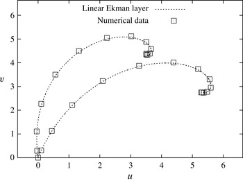
Sample Ekman spiral profiles, i.e. projections of the vertical profiles of the horizontal velocities
 $u(z),v(z)$
onto the
 $u,v$
plane, at two fixed horizontal locations in the lower viscous layer of the DNS at
 $RaE^{4/3}=20$
,
 $E=10^{-7}$
,
 ${\it\sigma}=7$
. The dashed line illustrates the analytic solution
 $(U_{0},V_{0})$
obtained from (3.37), (3.38). Open squares correspond to different vertical locations in the DNS boundary layer, computed using a vertical Chebyshev discretization with
 $385$
grid points.

The classical solution (Greenspan Reference Greenspan1969) is found within the Ekman layer at
 $Z=0$
and is given by
 $$\begin{eqnarray}\displaystyle & \displaystyle U_{0}^{(i)}(x,y,{\it\mu},t)=-\text{e}^{-{\it\mu}/\sqrt{2}}\left(U_{0}^{(o)}(x,y,0,t)\cos \frac{{\it\mu}}{\sqrt{2}}+V_{0}^{(o)}(x,y,0,t)\sin \frac{{\it\mu}}{\sqrt{2}}\right),\qquad & \displaystyle\end{eqnarray}$$
 $$\begin{eqnarray}\displaystyle & \displaystyle V_{0}^{(i)}(x,y,{\it\mu},t)=-\text{e}^{-{\it\mu}/\sqrt{2}}\left(V_{0}^{(o)}(x,y,0,t)\cos \frac{{\it\mu}}{\sqrt{2}}-U_{0}^{(o)}(x,y,0,t)\sin \frac{{\it\mu}}{\sqrt{2}}\right),\qquad & \displaystyle\end{eqnarray}$$
 $$\begin{eqnarray}\displaystyle & \displaystyle P_{1}^{(i)}(x,y,{\it\mu},t)=0. & \displaystyle\end{eqnarray}$$
Figure 5 illustrates sample boundary layer profiles obtained from DNS. The projected horizontal velocities are in perfect agreement with (3.37) and (3.38). These structures are robust throughout the boundary layer, thus providing confirmation of the existence of a linear Ekman layer (Stellmach et al. Reference Stellmach, Lischper, Julien, Vasil, Cheng, Ribeiro, King and Aurnou2014). Application of mass conservation (3.35) yields the inner and outer vertical velocities
 $$\begin{eqnarray}\displaystyle w & = & \displaystyle W_{0}^{(o)}(x,y,0,t)+{\it\epsilon}^{1/2}W_{1/2}^{(i)}(x,y,{\it\mu},t)\nonumber\\ \displaystyle & = & \displaystyle {\it\epsilon}^{1/2}\frac{1}{\sqrt{2}}{\it\zeta}_{0}^{(o)}(x,y,0,t)-{\it\epsilon}^{1/2}\frac{1}{\sqrt{2}}{\it\zeta}_{0}^{(o)}(x,y,0,t)\text{e}^{-{\it\mu}/\sqrt{2}}\left[\cos \frac{{\it\mu}}{\sqrt{2}}+\sin \frac{{\it\mu}}{\sqrt{2}}\right].\qquad\end{eqnarray}$$
As
 ${\it\mu}\rightarrow \infty$
, we see that
 $\lim \left(W_{1/2}^{(i)}\right)^{o}=0$
and hence that
 $$\begin{eqnarray}W_{0}^{(o)}(x,y,0,t)={\it\epsilon}^{1/2}{\textstyle \frac{1}{\sqrt{2}}}{\it\zeta}_{0}^{(o)}(x,y,0,t).\end{eqnarray}$$
This relation, often referred to as the Ekman pumping boundary condition, constitutes an exact parameterization of the linear Ekman layer in rotating RBC and represents Ekman pumping when
 $W_{0}^{(o)}>0$
and Ekman suction when
 $W_{0}^{(o)}<0$
. Hereafter, we do not distinguish between these two cases and refer to this phenomenon generically as Ekman pumping. Use of the Ekman pumping boundary condition alleviates the need to resolve the velocity dynamics that occurs within the Ekman layer. A similar analysis of the Ekman layer at
 $Z=1$
gives
 $$\begin{eqnarray}W_{0}^{(o)}(x,y,1,t)=-{\it\epsilon}^{1/2}{\textstyle \frac{1}{\sqrt{2}}}{\it\zeta}_{0}^{(o)}(x,y,1,t).\end{eqnarray}$$
Equations (3.41)–(3.42) exemplify the following important distinction between the asymptotic procedure performed here and the linear analyses of Niiler & Bisshopp (Reference Niiler and Bisshopp1965) and Heard & Veronis (Reference Heard and Veronis1971) which implicitly assume that
 $W_{1/2}^{(o)}=\pm (1/\sqrt{2}){\it\zeta}_{0}^{(o)}$
as opposed to
 $W_{0}^{(o)}=\pm {\it\epsilon}^{1/2}(1/\sqrt{2}){\it\zeta}_{0}^{(o)}$
(parameterized boundary conditions were not uncovered in these articles). The latter approach yields a perturbative analysis that captures a range of
 $\widetilde{Ra}$
for which the effect of Ekman pumping remains asymptotically close to the stress-free problem. However, for a sufficiently large
 $\widetilde{Ra}$
, determined below in § 3.3.1, the asymptotic expansion breaks down and becomes non-uniform. For completeness, this result is summarized in appendix A. We find that the maintenance of asymptotic uniformity requires that the pumping be elevated to contribute to the leading-order vertical velocity, as pursued here. This approach enables a complete exploration of Ekman pumping for all values of
 $\widetilde{Ra}$
for which the NH-QGEs remain valid.
Several studies (Barcilon Reference Barcilon1965; Faller & Kaylor Reference Faller and Kaylor1966; Dudis & Davis Reference Dudis and Davis1971) have established that solutions to the classical linear Ekman layer are unstable to small
 $\mathit{O}(E^{1/2}H)$
horizontal scale disturbances that evolve on rapid time scales that are filtered from the reduced dynamics. This occurs when the boundary layer Reynolds number
 $R_{E}=|\boldsymbol{U}_{0\bot }^{(o)}|E^{1/6}$
 ${\sim}55$
. Although this is within the realm of possibility for the rotationally constrained regime according to (3.26), to alter the pumping parameterization such an instability must also reach amplitudes comparable to the bulk vorticity. No evidence of this is presently seen in DNS.
The Ekman layer solutions (3.37)–(3.38) together with the application of the exact parameterizations (3.41)–(3.42) indicate that the outer velocity fields
 $(\boldsymbol{U}_{0\bot }^{(o)},W_{0}^{(o)})$
can be continued uniformly to the computational boundaries at
 $Z=0,1$
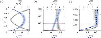
. Evidence for this two-layer structure is provided in figure 6, which illustrates the root mean square (r.m.s.) velocity profiles at various magnifications obtained from DNS at
 $\widetilde{Ra}=20,E=10^{-7},{\it\sigma}=7$
. Specifically, the figure demonstrates that the velocity structure is unaffected by the presence of the thermal boundary layer, defined in terms of the maxima of the r.m.s. of
 ${\it\theta}$
(purple line, plot (b)). These results suggest that Ekman layers in DNS of rotating RBC may be replaced by the parameterized pumping boundary conditions
 $$\begin{eqnarray}w(x,y,0,t)={\it\epsilon}^{1/2}{\textstyle \frac{1}{\sqrt{2}}}{\it\zeta}(x,y,0,t),\quad w(x,y,1,t)=-{\it\epsilon}^{1/2}{\textstyle \frac{1}{\sqrt{2}}}{\it\zeta}(x,y,1,t).\end{eqnarray}$$
Stellmach et al. (Reference Stellmach, Lischper, Julien, Vasil, Cheng, Ribeiro, King and Aurnou2014) have demonstrated the accuracy of this boundary layer parameterization via comparison of the heat transport obtained from DNS with no-slip boundaries and DNS where the Ekman pumping conditions are used. With all other details being identical in the two DNS studies, excellent quantitative agreement is reached. This result establishes that it is the presence of Ekman layers that is responsible for the strong differences in heat transport observed between stress-free and no-slip boundaries (figure 3).
Root mean square velocity profiles obtained via DNS with no-slip boundaries at
 $\widetilde{Ra}=20$
,
 $E=10^{-7}$
,
 ${\it\sigma}=7$
. The blue solid vertical line is the r.m.s. horizontal velocity
 $\sqrt{\overline{u_{\bot }^{2}}}$
and the black solid vertical line is the r.m.s. vertical velocity
 $\sqrt{\overline{w^{2}}}$
. Shaded regions denote the variance obtained from a time series. (a) Entire layer, (b) magnification of the
 $\mathit{O}(E^{1/3}H)$
thermal boundary layer scale and (c) magnification of the
 $\mathit{O}(E^{1/2}H)$
lower Ekman boundary layer. The Ekman boundary layer is delineated by the red horizontal dashed line, while the fluctuating thermal boundary layer (which has no visible effect on the velocity profiles) is delineated by the purple horizontal dashed line. The numerical grid points are marked by square and circular symbols in (c). The bulk velocity profile plotted in (a) transitions at the Ekman layer illustrated in (c).

The inner component of the pumping velocity
 $W_{1/2}^{(i)}$
defined in (3.40) gives rise to an inner temperature fluctuation
 ${\it\Theta}^{\prime (i)}$
satisfying
 $$\begin{eqnarray}W_{1/2}^{(i)}\partial _{Z}\overline{{\it\Theta}}_{0}^{(o)}(0)=\frac{1}{{\it\sigma}}\partial _{{\it\mu}{\it\mu}}{\it\Theta}_{5/2}^{\prime (i)}.\end{eqnarray}$$
Utilizing (3.40), the solution to this equation is given by
 $$\begin{eqnarray}{\it\Theta}_{5/2}^{\prime (i)}(x,y,{\it\mu},t)=-\frac{1}{\sqrt{2}}\text{e}^{-{\it\mu}/\sqrt{2}}\left[\cos \frac{{\it\mu}}{\sqrt{2}}-\sin \frac{{\it\mu}}{\sqrt{2}}\right]{\it\zeta}_{0}^{(o)}(0)\partial _{Z}\overline{{\it\Theta}}_{0}^{(o)}(0).\end{eqnarray}$$
The limiting values as
 ${\it\mu}\rightarrow 0$
and
 ${\it\mu}\rightarrow \infty$
are
 $$\begin{eqnarray}{\it\Theta}^{\prime (i)}(0)=-{\it\epsilon}^{5/2}{\textstyle \frac{1}{\sqrt{2}}}{\it\zeta}_{0}^{(o)}(0)\,\partial _{Z}\overline{{\it\Theta}}_{0}^{(o)}(0),\quad {\it\Theta}^{\prime (i)}\left({\it\mu}\rightarrow \infty \right)=0.\end{eqnarray}$$
It thus follows that the temperature fluctuations within the Ekman layer are of magnitude
 ${\it\Theta}^{\prime (i)}=\mathit{O}({\it\epsilon}^{5/2}{\it\zeta}_{0}^{(o)}(0)\,\partial _{Z}\overline{{\it\Theta}}_{0}^{(o)}(0))$
. This observation yields an estimate of the convective heat transport,
 $$\begin{eqnarray}{\it\epsilon}^{3}W_{1/2}^{(i)}(0){\it\Theta}_{5/2}^{\prime (i)}(0)\sim {\it\epsilon}^{3}({\it\zeta}_{0}^{(o)}(0))^{2}\,\partial _{Z}\overline{{\it\Theta}}_{0}^{(o)}(0),\end{eqnarray}$$
which is smaller in magnitude by a factor of
 $\mathit{O}({\it\epsilon}^{2})$
when compared with that occurring in the convective interior, namely
 ${\it\epsilon}(W_{0}^{(o)}{\it\Theta}_{1}^{\prime (o)})$
. We can thus conclude that the observed enhancement of heat flux as measured by
 $Nu$
(figure 3) cannot occur directly within the Ekman layer given the vorticity bound (3.26).
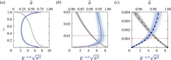
Root mean square temperature profiles obtained via DNS with no-slip boundaries at
 $\widetilde{Ra}=Ra\,E^{4/3}=20$
,
 $E=10^{-7}$
,
 ${\it\sigma}=7$
. The blue solid vertical line is the r.m.s. temperature
 $E^{-1/3}\sqrt{\overline{{\it\theta}^{\prime 2}}}$
and the black solid vertical line is the r.m.s. mean temperature
 $\overline{{\it\theta}}$
. Shaded regions denote the variance obtained from a time series. (a) Entire layer, (b) magnification of the
 $\mathit{O}(E^{1/3}H)$
thermal boundary layer scale and (c) magnification of the Ekman boundary layer. The fluctuating thermal boundary layer is delineated by the purple horizontal dashed line, while the Ekman boundary layer is delineated by the red horizontal dashed line. The numerical grid points are marked by square and circular symbols in (c). The thermal profile exhibits no visible boundary layer structure on the Ekman layer scale (c).

Inspection of the r.m.s. thermal profiles at increasing magnification obtained at
 $E=10^{-7}$
shows no visible boundary layer structure in the vicinity of the Ekman layer (cf. figure 7
b,c). The r.m.s. profiles reveal that the thermal boundary layer extends much farther into the interior than the Ekman layer observed in figure 6. Indeed, we recall that the mean temperature
 $\overline{{\it\Theta}}_{0}^{(o)}(Z,{\it\tau})$
is an outer variable independent of the fast spatial variables
 ${\it\mu}$
and
 $z$
(Sprague et al.
Reference Sprague, Julien, Knobloch and Werne2006).
3.2.1 The significance of Ekman pumping
It now remains to determine the nature of the thermal response in the immediate vicinity of the Ekman layer. Focusing again on the lower boundary, this requires consideration of how the reduced outer equation for the temperature fluctuations (3.18) can be continued to the physical boundaries. On Taylor-expanding all fluid variables within the Ekman layer, the outer component of the pumping velocity
 $W_{0}^{(o)}(0)$
induces outer temperature fluctuations
 ${\it\Theta}_{1}^{\prime (o)}(0)$
that satisfy
 $$\begin{eqnarray}(\partial _{t}+\boldsymbol{U}_{0\bot }^{(o)}(0)\boldsymbol{\cdot }\boldsymbol{{\rm\nabla}}_{\bot }){\it\Theta}_{1}^{\prime (o)}(0)+\frac{{\it\epsilon}^{1/2}}{\sqrt{2}}{\it\zeta}_{0}^{(o)}(0)\partial _{Z}\overline{{\it\Theta}}_{0}^{(o)}(0)=\frac{1}{{\it\sigma}}{\rm\nabla}_{\bot }^{2}{\it\Theta}_{1}^{\prime (o)}(0).\end{eqnarray}$$
Here, we have set
 $W_{0}^{(o)}(0)=({\it\epsilon}^{1/2}/\sqrt{2}){\it\zeta}_{0}^{(o)}(0)$
.
In a statistically stationary state, averaging the equation for the thermal variance obtained from (3.48) gives the balance
 $$\begin{eqnarray}\frac{{\it\epsilon}^{1/2}}{\sqrt{2}}\overline{\overline{{\it\Theta}_{1}^{\prime (o)}(0){\it\zeta}_{0}^{(o)}(0)}}^{\mathscr{T}}\partial _{Z}\overline{{\it\Theta}}_{0}^{(o)}(0)=-\frac{1}{{\it\sigma}}\overline{\overline{|\boldsymbol{{\rm\nabla}}_{\bot }{\it\Theta}_{1}^{\prime (o)}(0)|^{2}}}^{\mathscr{T}}.\end{eqnarray}$$
Clearly, in contrast to stress-free boundaries where
 ${\it\Theta}_{1}^{\prime (o)}(0)\equiv 0$
, pumping induces the enhanced thermal response
 $$\begin{eqnarray}{\it\Theta}_{1}^{\prime (o)}(0)=\mathit{O}({\it\epsilon}^{1/2}{\it\zeta}_{0}^{(o)}(0)\partial _{Z}\overline{{\it\Theta}}_{0}^{(o)}(0))\end{eqnarray}$$
immediately outside the Ekman layer. The associated enhancement in the convective flux is estimated as
 $$\begin{eqnarray}\overline{W_{0}^{(o)}(0){\it\Theta}_{1}^{\prime (o)}(0)}=\mathit{O}({\it\epsilon}({\it\zeta}_{0}^{(o)}(0))^{2}\partial _{Z}\overline{{\it\Theta}}_{0}^{(o)}(0)).\end{eqnarray}$$
This equation shows that the convective flux induced by Ekman pumping becomes as important as the conductive transport
 $-\partial _{Z}\overline{{\it\Theta}}_{0}^{(o)}(0)$
when
 $$\begin{eqnarray}{\it\zeta}_{0}^{(o)}(0)=\mathit{O}({\it\epsilon}^{-1/2}).\end{eqnarray}$$
This threshold is always achieved within the regime of asymptotic validity of the NH-QGEs that demands
 ${\it\zeta}_{0}^{(o)}(0)=o({\it\epsilon}^{-1})$
(see § 3.1.1). This result also indicates that the differences between stress-free and no-slip boundary conditions are asymptotically
 $\mathit{O}({\it\epsilon}^{1/2})$
-small for rotationally constrained RBC when
 ${\it\zeta}_{0}^{(o)}(0)=o\left({\it\epsilon}^{-1/2}\right)$
(see appendix A). Strong
 $\mathit{O}(1)$
departures are predicted to occur in the range
 $$\begin{eqnarray}\mathit{O}({\it\epsilon}^{-1/2})\leqslant {\it\zeta}_{0}^{(o)}(0)<\mathit{O}({\it\epsilon}^{-1}).\end{eqnarray}$$
As we show below, the vast majority of laboratory experiments and DNS studies fall within this range.
3.3 The middle region: thermal wind layer
It is evident from (3.50) that
 ${\it\Theta}_{1}^{\prime (o)}(0)$
cannot satisfy the thermal boundary condition
 ${\it\Theta}^{\prime (o)}(0)=0$
, implying that the thermal response to Ekman pumping in the NH-QGEs requires a boundary layer regularization. However, temperature fluctuations
 ${\it\Theta}^{\prime (i)}(0)=\mathit{O}({\it\epsilon}^{5/2}{\it\Theta}_{1}^{\prime (0)}(0))$
within the Ekman layer are too small to provide compensation (see (3.46a,b
)). This indicates the existence of a middle
 $(m)$
region
 $\mathit{O}({\it\epsilon})$
in depth (Heard & Veronis Reference Heard and Veronis1971).
Within the middle region, the inner
 $(i)$
variables are identically zero and the bulk variables achieve their boundary values. We introduce an expansion of the form
 $$\begin{eqnarray}\displaystyle \boldsymbol{u}^{(m)}=\lim (\boldsymbol{u})^{m}=\boldsymbol{U}_{0}^{(m)}+{\it\epsilon}\boldsymbol{U}_{1}^{(m)}+{\it\epsilon}^{2}\boldsymbol{U}_{2}^{(m)}+\cdots \,, & & \displaystyle\end{eqnarray}$$
and retain geostrophic balance as the leading-order fluctuation balance in the middle region, as in (3.12). Thus, the Proudman–Taylor constraint
 $\partial _{z}(\boldsymbol{U}_{0}^{(m)},P_{1}^{(m)})=0$
implies
 $(\boldsymbol{U}_{0}^{(m)},P_{1}^{(m)})=0$
. Departures from the NH-QGEs (3.16)–(3.18), (3.11) and (3.19) due to Ekman pumping can be deduced from the following prognostic equations:
 $$\begin{eqnarray}\displaystyle & \displaystyle D_{0t}^{\bot }\boldsymbol{U}_{0\bot }^{\prime (o)}+\widehat{\boldsymbol{z}}\times \boldsymbol{U}_{1}=-\boldsymbol{{\rm\nabla}}_{\bot }P_{2}^{\prime }+{\rm\nabla}_{\bot }^{2}\boldsymbol{U}_{0\bot }^{\prime (o)}, & \displaystyle\end{eqnarray}$$
 $$\begin{eqnarray}\displaystyle & \displaystyle D_{0t}^{\bot }W_{0}^{\prime (o)}=-\partial _{z}P_{2}^{(m)}-\partial _{Z}P_{1}^{(o)}+\frac{\widetilde{Ra}}{{\it\sigma}}{\it\Theta}_{1}+{\rm\nabla}_{\bot }^{2}W_{0}^{\prime (o)}, & \displaystyle\end{eqnarray}$$
 $$\begin{eqnarray}\displaystyle & \displaystyle D_{0t}^{\bot }{\it\Theta}_{1}+W_{0}^{\prime (o)}(\partial _{z}{\it\Theta}_{1}^{(m)}+\partial _{Z}\overline{{\it\Theta}}_{0}^{(o)})=\frac{1}{{\it\sigma}}{\rm\nabla}^{2}{\it\Theta}_{1}, & \displaystyle\end{eqnarray}$$
 $$\begin{eqnarray}\displaystyle & \displaystyle \boldsymbol{{\rm\nabla}}\boldsymbol{\cdot }\boldsymbol{U}_{1}+\partial _{Z}W_{0}^{\prime (o)}=0. & \displaystyle\end{eqnarray}$$
Variables without superscripts contribute to both the outer
 $(o)$
and middle
 $(m)$
regions and can be separated by taking the limits (3.7)–(3.9). It should be noted that (3.57) contains the three-dimensional (3D) Laplacian
 ${\rm\nabla}^{2}\equiv \partial _{x}^{2}+\partial _{y}^{2}+\partial _{z}^{2}$
.
Inspection of the momentum equation (3.55) and the continuity equation (3.58) in the middle region yields the hydrostatic thermal wind balance
 $$\begin{eqnarray}\displaystyle & \displaystyle \widehat{\boldsymbol{z}}\times \boldsymbol{U}_{1}^{\prime (m)}=-\boldsymbol{{\rm\nabla}}_{\bot }P_{2}^{\prime (m)}, & \displaystyle\end{eqnarray}$$
 $$\begin{eqnarray}\displaystyle & \displaystyle \partial _{z}P_{2}^{\prime (m)}=\frac{\widetilde{Ra}}{{\it\sigma}}{\it\Theta}_{1}^{\prime (m)}, & \displaystyle\end{eqnarray}$$
 $$\begin{eqnarray}\boldsymbol{{\rm\nabla}}_{\bot }\boldsymbol{\cdot }\boldsymbol{U}_{1}^{\prime (m)}=0\quad \text{and}\quad W_{1}^{\prime (m)}\equiv 0,\end{eqnarray}$$
from which we find
 $$\begin{eqnarray}\partial _{z}\boldsymbol{U}_{1\bot }^{\prime (m)}=\frac{\widetilde{Ra}}{{\it\sigma}}\boldsymbol{{\rm\nabla}}^{\bot }{\it\Theta}_{1}^{\prime (m)},\quad \text{s.t. }\boldsymbol{U}_{1\bot }^{\prime (m)}=\boldsymbol{{\rm\nabla}}^{\bot }{\it\Psi}_{1}^{(m)},\quad P_{2}^{\prime (m)}={\it\Psi}_{1}^{(m)}.\end{eqnarray}$$
The upper and lower middle layer convective dynamics is thus completely reduced to the determination of
 ${\it\Theta}_{1}^{\prime (m)}$
, which from (3.57) evolves according to
 $$\begin{eqnarray}\displaystyle D_{0t}^{\bot }{\it\Theta}_{1}^{\prime (m)}+W_{0}^{\prime (o)}\partial _{z}\left(\overline{{\it\Theta}}_{1}^{(m)}+{\it\Theta}_{1}^{\prime (m)}\right)-\partial _{z}\left(\overline{W_{0}^{\prime ^{(o)}}{\it\Theta}_{1}^{\prime ^{(m)}}}\right)=\frac{1}{{\it\sigma}}{\rm\nabla}^{2}{\it\Theta}_{1}^{\prime (m)}. & & \displaystyle\end{eqnarray}$$
This couples to the mean state via
 $$\begin{eqnarray}\displaystyle & \displaystyle \partial _{z}\overline{P}_{2}^{(m)}=\frac{\widetilde{Ra}}{{\it\sigma}}\overline{{\it\Theta}}_{1}^{(m)}, & \displaystyle\end{eqnarray}$$
 $$\begin{eqnarray}\displaystyle & \displaystyle \partial _{t}\overline{{\it\Theta}}_{1}^{(m)}+\partial _{z}\left(\overline{W_{0}^{\prime ^{(o)}}{\it\Theta}_{1}^{\prime ^{(m)}}}\right)=\frac{1}{{\it\sigma}}\partial _{zz}\overline{{\it\Theta}}_{1}^{(m)}. & \displaystyle\end{eqnarray}$$
Equations (3.63) and (3.65) yield the thermal variance relation
 $$\begin{eqnarray}\frac{1}{2}\partial _{t}\left\langle \left(\overline{{\it\Theta}}_{1}^{(m)}\right)^{2}+\overline{\left({\it\Theta}_{1}^{\prime (m)}\right)^{2}}\right\rangle =-\frac{1}{{\it\sigma}}\left\langle \left(\partial _{z}\overline{{\it\Theta}}_{1}^{(m)}\right)^{2}+\overline{\left(\partial _{z}{\it\Theta}_{1}^{\prime (m)}\right)^{2}}\right\rangle .\end{eqnarray}$$
It follows that non-zero values of
 $\overline{{\it\Theta}}_{1}^{(m)},{\it\Theta}_{1}^{\prime (m)}$
only exist in the middle region if they are sustained through the regularizing boundary conditions
 $$\begin{eqnarray}\displaystyle {\it\Theta}_{1}^{\prime (o)}+{\it\Theta}_{1}^{\prime (m)}=0,\quad {\it\Theta}_{1}^{\prime (m)}(z\rightarrow \infty )=0, & & \displaystyle\end{eqnarray}$$
 $$\begin{eqnarray}\displaystyle \overline{{\it\Theta}}_{1}^{(o)}+\overline{{\it\Theta}}_{1}^{(m)}=0,\quad \overline{{\it\Theta}}_{1}^{(m)}(z\rightarrow \infty )=0 & & \displaystyle\end{eqnarray}$$
at
 $Z=0$
or
 $1$
. Importantly, we conclude from (3.67), (3.68) that equations (3.63), (3.65) are fully coupled to the interior dynamics. Averaging (3.65) over
 $t$
, followed by integration with respect to
 $z$
, generates the heat transport relation
 $$\begin{eqnarray}{\it\sigma}\left(\overline{\overline{W_{0}^{\prime (o)}{\it\Theta}_{1}^{\prime (m)}}}^{\mathscr{T}}\right)-\partial _{z}\overline{\overline{{\it\Theta}}_{1}^{(m)}}^{\mathscr{T}}=0.\end{eqnarray}$$
By application of the outer limit to this equation, the constant of integration must be identically zero. This relation indicates that there is no net heat flux associated with the middle layer dynamics.
We now see that within the upper and lower middle regions relation (2.5) yields
 $$\begin{eqnarray}Nu={\it\sigma}\left(\overline{\overline{W_{0}^{\prime (o)}\left({\it\Theta}_{1}^{\prime (o)}+{\it\Theta}_{1}^{\prime (m)}\right)}}^{\mathscr{T}}\right)-\left(\partial _{Z}\overline{{\it\Theta}}_{0}^{(o)}+\partial _{z}\overline{\overline{{\it\Theta}}_{1}^{(m)}}^{\mathscr{T}}\right).\end{eqnarray}$$
Given (3.69), we find
 $$\begin{eqnarray}Nu={\it\sigma}\left(\overline{\overline{W_{0}^{\prime (o)}{\it\Theta}_{1}^{\prime (o)}}}^{\mathscr{T}}\right)-\partial _{Z}\overline{{\it\Theta}}_{0}^{(o)},\end{eqnarray}$$
valid at every vertical level. This result states that the heat transport within the fluid layer is determined entirely within the bulk. Moreover, (3.48), (3.50) and (3.51) now imply that any enhancement in heat transport is entirely due to buoyancy production in
 ${\it\Theta}_{1}^{\prime (o)}$
arising through the nonlinear advection of the mean temperature gradient
 ${\it\epsilon}^{1/2}{\it\zeta}_{0}^{\prime (o)}\partial _{Z}\overline{{\it\Theta}}_{0}^{(o)}/\sqrt{2}$
generated by Ekman pumping.
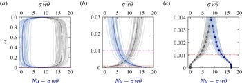
Convective flux
 ${\it\sigma}\overline{w{\it\theta}}$
(vertical dashed line) and mean temperature gradient
 $-\partial _{z}\overline{{\it\theta}}=Nu-{\it\sigma}\overline{w{\it\theta}}$
(vertical solid line) obtained for DNS with no-slip boundaries at
 $\widetilde{Ra}=20,E=10^{-7},{\it\sigma}=7$
and average
 $Nu=17$
. Shaded regions denote the variance obtained from a time series. (a) Entire layer, (b) magnification of the
 $\mathit{O}(E^{1/3}H)$
thermal boundary layer scale and (c) magnification of the Ekman boundary layer. The fluctuating thermal boundary layer is delineated by the purple horizontal dashed line, while the Ekman boundary layer is delineated by the red horizontal dashed line. The numerical grid points are marked by square and circular symbols. Equipartition is reached within the thermal wind layer (b).

Direct numerical simulation results indicate that equipartition between convective and conductive heat transport is achieved within the middle layer (see figure 8). For comparison, for stress-free boundary conditions, equipartition occurs at a vertical depth well outside that associated with the middle layer.
3.3.1 Estimation of the transition threshold,
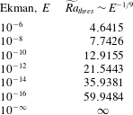
 $\widetilde{Ra}_{thres}$

In the following, we determine the threshold Rayleigh number
 $\widetilde{Ra}_{thres}$
at which Ekman pumping gains significance according to the criterion
 ${\it\zeta}_{0}^{(o)}(0)\sim {\it\epsilon}^{-1/2}$
in (3.53). This is achieved by assessing the
 $\widetilde{Ra}$
dependence of the outer fluid variables prior to the transition threshold where stress-free and no-slip boundary conditions are presumed to be asymptotically indistinguishable at leading order. Direct numerical simulations at
 $E=10^{-7}$
(Stellmach et al.
Reference Stellmach, Lischper, Julien, Vasil, Cheng, Ribeiro, King and Aurnou2014, figure 3) have established that Ekman pumping has a significant effect on the heat transport within the laminar CTC regime. We therefore make an a priori assumption that the transition occurs within this regime. Simulations of the NH-QGEs for rotating Rayleigh–Bénard convection (Julien et al.
Reference Julien, Rubio, Grooms and Knobloch2012b
) have established that the dynamics within the CTC regime exhibits power law scalings with respect to
 $\widetilde{Ra}$
in both the bulk and the thermal boundary layer. Hence, we pose the following scaling relations:
 $$\begin{eqnarray}\displaystyle \left.\begin{array}{@{}c@{}}\displaystyle W_{0}^{(o)}=\widetilde{Ra}^{{\hat{w}}}\widehat{W}_{0}^{(o)},\quad {\it\Psi}_{0}^{(o)}=\widetilde{Ra}^{\hat{{\it\psi}}}\widehat{{\it\Psi}}_{0}^{(o)},\quad {\it\zeta}_{0}^{(o)}=\widetilde{Ra}^{\hat{{\it\zeta}}}\widehat{{\it\zeta}}_{0}^{(o)},\quad {\it\Theta}_{1}^{\prime (o)}=\widetilde{Ra}^{\hat{{\it\theta}}}\widehat{{\it\Theta}}_{1}^{(o)},\\ \displaystyle \partial _{Z}\overline{{\it\Theta}}_{0}^{(o)}=\widetilde{Ra}^{\hat{\text{d}t}}\widehat{\partial _{Z}\overline{{\it\Theta}}}_{0}^{(o)},\quad Nu=\widetilde{Ra}^{\hat{{\it\beta}}}\widehat{Nu}.\end{array}\right\} & & \displaystyle\end{eqnarray}$$
On noting that
 $\partial _{t},\boldsymbol{{\rm\nabla}}_{\bot },\partial _{Z}=\mathit{O}(1)$
in the core region and that the CTC structures are known to be axisymmetric to leading order (Grooms et al.
Reference Grooms, Julien, Weiss and Knobloch2010), the following balances hold in the NH-QGEs:
 $$\begin{eqnarray}\displaystyle & \displaystyle \partial _{t}{\it\zeta}_{0}^{(o)}\sim -\partial _{Z}W_{0}^{(o)}\sim {\rm\nabla}_{\bot }^{2}{\it\zeta}_{0}^{(o)}, & \displaystyle\end{eqnarray}$$
 $$\begin{eqnarray}\displaystyle & \displaystyle \partial _{t}W_{0}^{(o)}\sim \partial _{Z}{\it\Psi}_{1}^{(o)}\sim \widetilde{Ra}{\it\Theta}_{1}^{\prime (o)}\sim {\rm\nabla}_{\bot }^{2}W_{0}^{(o)}, & \displaystyle\end{eqnarray}$$
 $$\begin{eqnarray}\displaystyle & \displaystyle \partial _{t}{\it\Theta}_{1}^{\prime (o)}\sim W_{0}^{(o)}\partial _{Z}\overline{{\it\Theta}}_{0}^{(o)}\sim \displaystyle \frac{1}{{\it\sigma}}{\rm\nabla}_{\bot }^{2}{\it\Theta}_{1}^{\prime (o)}, & \displaystyle\end{eqnarray}$$
 $$\begin{eqnarray}\displaystyle & \displaystyle {\it\sigma}\overline{\overline{W_{0}^{(o)}{\it\Theta}_{1}^{\prime (o)}}}^{\mathscr{T}}\sim Nu. & \displaystyle\end{eqnarray}$$
The algebraic equations satisfied by the exponents defined in (3.72) are given by
 $$\begin{eqnarray}{\hat{w}}=\hat{{\it\psi}}=\hat{{\it\zeta}}=1+\hat{{\it\theta}},\quad {\hat{w}}+\hat{\text{d}t}=\hat{{\it\theta}},\quad {\hat{w}}+\hat{{\it\theta}}=\hat{{\it\beta}}.\end{eqnarray}$$
On assuming that
 $\hat{{\it\beta}}$
is known empirically, we obtain
 $$\begin{eqnarray}{\hat{w}}=\hat{{\it\psi}}=\hat{{\it\zeta}}=\frac{\hat{{\it\beta}}+1}{2},\quad \hat{{\it\theta}}=\frac{\hat{{\it\beta}}-1}{2},\quad \hat{\text{d}t}=-1.\end{eqnarray}$$
This result indicates that as the amplitude of convection intensifies with increasing
 $\widetilde{Ra}$
, the mean bulk temperature gradient approaches an increasingly well-mixed interior according to
 $\widetilde{Ra}^{-1}$
. This is a well-established result of the CTC regime (Sprague et al.
Reference Sprague, Julien, Knobloch and Werne2006; Julien et al.
Reference Julien, Rubio, Grooms and Knobloch2012b
) that is confirmed by the reduced simulations (Julien et al.
Reference Julien, Rubio, Grooms and Knobloch2012b
), which yield
 $Nu\sim \widetilde{Ra}^{2.1}$
together with the bulk scalings
 $$\begin{eqnarray}\displaystyle \partial _{Z}\overline{{\it\Theta}}_{0}^{(o)}\sim \widetilde{Ra}^{-0.96},\quad W_{0}^{(o)}=\widetilde{Ra}^{1.53},\quad {\it\zeta}_{0}^{(o)}\sim \widetilde{Ra}^{1.55},\quad {\it\Theta}_{1}^{\prime (o)}\sim \widetilde{Ra}^{0.62} & & \displaystyle\end{eqnarray}$$
evaluated at
 $Z=1/2$
for all variables except vorticity which is evaluated at
 $Z=3/4$
owing to its antisymmetry. The empirically measured scalings are in good quantitative agreement with the choice
 $\hat{{\it\beta}}\approx 2$
, giving
 $$\begin{eqnarray}Nu\sim \widetilde{Ra}^{2},\quad W_{0}^{(o)}={\it\zeta}_{0}^{(o)}\sim \widetilde{Ra}^{3/2},\quad {\it\Theta}_{1}^{(o)}\sim \widetilde{Ra}^{1/2}.\end{eqnarray}$$
In the thermal boundary layers, where it is once again assumed that
 $\partial _{t},\boldsymbol{{\rm\nabla}}_{\bot }=\mathit{O}(1)$
, but now
 $\partial _{Z}=\widetilde{Ra}^{\hat{{\it\eta}}}\gg 1$
, the following balances hold:
 $$\begin{eqnarray}\displaystyle & \displaystyle \partial _{t}{\it\zeta}_{0}^{(o)}\sim -\partial _{Z}W_{0}^{(o)}\sim {\rm\nabla}_{\bot }^{2}{\it\zeta}_{0}^{(o)}, & \displaystyle\end{eqnarray}$$
 $$\begin{eqnarray}\displaystyle & \displaystyle \partial _{Z}{\it\Psi}_{1}^{(o)}\sim \widetilde{Ra}{\it\Theta}_{1}^{\prime (o)}, & \displaystyle\end{eqnarray}$$
 $$\begin{eqnarray}\displaystyle & \displaystyle \partial _{t}{\it\Theta}_{1}^{\prime (o)}\sim W_{0}^{(o)}\partial _{Z}\overline{{\it\Theta}}_{0}^{(o)}\sim \displaystyle \frac{1}{{\it\sigma}}{\rm\nabla}_{\bot }^{2}{\it\Theta}_{1}^{\prime (o)}, & \displaystyle\end{eqnarray}$$
 $$\begin{eqnarray}\displaystyle & \displaystyle {\it\sigma}\overline{\overline{W_{0}^{(o)}{\it\Theta}_{1}^{\prime (o)}}}^{\mathscr{T}}\sim \partial _{Z}\overline{{\it\Theta}}_{0}^{(o)}\sim Nu. & \displaystyle\end{eqnarray}$$
The algebraic equations satisfied by the exponents defined in (3.72) now satisfy
 $$\begin{eqnarray}\hat{{\it\eta}}+{\hat{w}}=\hat{{\it\psi}}=\hat{{\it\zeta}},\quad \hat{{\it\eta}}+\hat{{\it\psi}}=1+\hat{{\it\theta}},\quad {\hat{w}}+\hat{\text{d}t}=\hat{{\it\theta}},\quad {\hat{w}}+\hat{{\it\theta}}=\hat{\text{d}t}=\hat{{\it\beta}},\end{eqnarray}$$
with the solution
 $$\begin{eqnarray}\hat{{\it\eta}}=\hat{{\it\psi}}=\hat{{\it\zeta}}=\frac{\hat{{\it\beta}}+1}{2},\quad {\hat{w}}=0,\quad \hat{{\it\theta}}=\hat{\text{d}t}=\hat{{\it\beta}}.\end{eqnarray}$$
From (3.78) and (3.86), it now follows that the vorticity satisfies
 $$\begin{eqnarray}{\it\zeta}_{0}^{(o)}\sim \widetilde{Ra}^{(\hat{{\it\beta}}+1)/2}\widehat{{\it\zeta}}_{0}^{(o)},\end{eqnarray}$$
and hence that (see (3.53))
 $$\begin{eqnarray}{\it\zeta}_{0}^{(o)}(0)\sim {\it\epsilon}^{-1/2}\Rightarrow \widetilde{Ra}_{thres}=\mathit{O}({\it\epsilon}^{-1/(\hat{{\it\beta}}+1)})=\mathit{O}(E^{-1/(3(\hat{{\it\beta}}+1))}).\end{eqnarray}$$
Specifically, for the empirically observed CTC value of
 $\hat{{\it\beta}}\approx 2$
,
 $$\begin{eqnarray}\widetilde{Ra}_{thres}=\mathit{O}({\it\epsilon}^{-1/3})=\mathit{O}(E^{-1/9}).\end{eqnarray}$$
At
 $E=10^{-7}$
this gives a value
 $\widetilde{Ra}_{thres}\sim 6.0$
. This is of the same magnitude as the critical Rayleigh number
 $\widetilde{Ra}_{c}=8.05$
(Heard & Veronis Reference Heard and Veronis1971), indicating an immediate departure from the stress-free case. This is a conclusion borne out by the recent DNS (figure 3(b)). At lower values of
 $E$
, it is found that
 $\widetilde{Ra}_{thres}>\widetilde{Ra}_{c}$
. From the interior and boundary layer scaling exponents (3.78) and (3.86), we also estimate the magnitude of Ekman pumping normalized by the midplane velocity as
 $$\begin{eqnarray}S=\frac{E^{1/6}{\it\zeta}_{0}^{(o)}(0)/\sqrt{2}}{w_{0}^{(o)}(\frac{1}{2})}=\mathit{O}(E^{1/6}),\end{eqnarray}$$
thus confirming the empirical DNS results (see figure 5 of Stellmach et al. (Reference Stellmach, Lischper, Julien, Vasil, Cheng, Ribeiro, King and Aurnou2014)).
4 Composite reduced NH-QGEs
The findings of § 3 are now combined to deduce a composite reduced model capable of capturing the thermal effect of Ekman pumping in a single domain
 $Z=[0,1]$
. This is accomplished by reconstituting the fluid variables in each region as defined in (3.6), with the exception that the Ekman layer is now parameterized. For convenience, we first summarize the reduced asymptotic equations of the outer and middle regions.
In the presence of no-slip boundary conditions, we have established that the outer, i.e. bulk, region is described by the reduced NH-QGE system:
outer region:
 $$\begin{eqnarray}\displaystyle & \displaystyle \overline{\boldsymbol{U}}_{0}^{(o)}\equiv 0,\quad \boldsymbol{U}_{0}^{\prime (o)}=\boldsymbol{{\rm\nabla}}^{\bot }{\it\Psi}_{0}^{(o)}+W_{0}^{(o)}\widehat{\boldsymbol{z}},\quad P^{(o)}=\overline{P}_{0}^{(o)}+{\it\epsilon}{\it\Psi}_{0}^{(o)},\quad {\it\Theta}^{(o)}=\overline{{\it\Theta}}_{0}^{(o)}+{\it\epsilon}{\it\Theta}_{1}^{\prime (o)}, & \displaystyle \nonumber\\ \displaystyle & & \displaystyle\end{eqnarray}$$
with a hydrostatically evolving mean component
 $$\begin{eqnarray}\displaystyle \left.\begin{array}{@{}c@{}}\partial _{Z}\overline{P}_{0}=\displaystyle \frac{\widetilde{Ra}}{{\it\sigma}}\overline{{\it\Theta}}_{0},\\ \partial _{{\it\tau}}\overline{{\it\Theta}}_{0}^{(o)}+\partial _{Z}\left(\overline{\overline{W_{0}^{(o)}{\it\Theta}_{1}^{\prime (o)}}}^{\mathscr{T}}\right)=\displaystyle \frac{1}{{\it\sigma}}\partial _{ZZ}\overline{{\it\Theta}}_{0}^{(o)},\\ \overline{{\it\Theta}}_{0}^{(o)}(0)=1,\quad \overline{{\it\Theta}}_{0}^{(o)}(1)=0,\end{array}\right\} & & \displaystyle\end{eqnarray}$$
with fixed mean temperature boundaries. The quasi-geostrophically evolving fluctuating components are given by
 $$\begin{eqnarray}\displaystyle \left.\begin{array}{@{}c@{}}D_{0t}^{\bot }{\it\zeta}_{0}^{(o)}-\partial _{Z}W_{0}^{(o)}={\rm\nabla}_{\bot }^{2}{\it\zeta}_{0}^{(o)},\\ D_{0t}^{\bot }W_{0}^{(o)}+\partial _{Z}{\it\Psi}_{0}^{(o)}=\displaystyle \frac{\widetilde{Ra}}{{\it\sigma}}{\it\Theta}_{1}^{\prime (o)}+{\rm\nabla}_{\bot }^{2}W_{0}^{(o)},\\ D_{0t}^{\bot }{\it\Theta}_{1}^{\prime (o)}+W_{0}^{(o)}\partial _{Z}\overline{{\it\Theta}}_{0}^{(o)}=\displaystyle \frac{1}{{\it\sigma}}{\rm\nabla}_{\bot }^{2}{\it\Theta}_{1}^{\prime (o)},\\ W_{0}^{(o)}(0)=\displaystyle \frac{{\it\epsilon}^{1/2}}{\sqrt{2}}{\it\zeta}_{0}^{(o)}(0),\quad W_{0}^{(o)}(1)=-\displaystyle \frac{{\it\epsilon}^{1/2}}{\sqrt{2}}{\it\zeta}_{0}^{(o)}(1),\end{array}\right\} & & \displaystyle\end{eqnarray}$$
with parameterized pumping boundary conditions. The requirement of zero thermal fluctuations on the boundaries was shown to require the introduction of a pair of middle boundary layer regions:
middle regions at
 $Z\equiv Z_{b}=0$
or 1:
 $$\begin{eqnarray}\displaystyle & \displaystyle \boldsymbol{U}^{\prime (m)}={\it\epsilon}\boldsymbol{{\rm\nabla}}^{\bot }{\it\Psi}_{1}^{(m)},\quad P^{(m)}={\it\epsilon}\left(\overline{P}_{1}^{(m)}+{\it\Psi}_{1}^{(m)}\right),\quad {\it\Theta}^{(m)}={\it\epsilon}\left(\overline{{\it\Theta}}_{1}^{(m)}+{\it\Theta}_{1}^{\prime (m)}\right),\qquad & \displaystyle\end{eqnarray}$$
with a hydrostatically evolving mean component
 $$\begin{eqnarray}\displaystyle \left.\begin{array}{@{}c@{}}\partial _{z}\overline{P}_{1}^{(m)}=\displaystyle \frac{\widetilde{Ra}}{{\it\sigma}}\overline{{\it\Theta}}_{1}^{(m)},\\ \partial _{t}\overline{{\it\Theta}}_{1}^{(m)}+\partial _{z}\left(\overline{W_{0}^{(o)}{\it\Theta}_{1}^{\prime (m)}}\right)=\displaystyle \frac{1}{{\it\sigma}}\partial _{zz}\overline{{\it\Theta}}_{1}^{(m)},\\ \overline{{\it\Theta}}_{1}^{(m)}(\infty )=0,\end{array}\right\} & & \displaystyle\end{eqnarray}$$
and a geostrophically evolving fluctuating component
 $\widehat{\boldsymbol{z}}\times \boldsymbol{U}_{1}^{\prime (m)}=-\boldsymbol{{\rm\nabla}}{\it\Psi}_{1}^{(m)}$
in thermal wind balance
 $$\begin{eqnarray}\displaystyle \left.\begin{array}{@{}c@{}}\partial _{z}{\it\Psi}_{1}^{(m)}=\displaystyle \frac{\widetilde{Ra}}{{\it\sigma}}{\it\Theta}_{1}^{\prime (m)},\\ D_{0t}^{\bot }{\it\Theta}_{1}^{\prime (m)}+W_{0}^{(o)}\partial _{z}\overline{{\it\Theta}}_{1}^{(m)}+\partial _{z}\left(W_{0}^{(o)}{\it\Theta}_{1}^{\prime (m)}-\overline{W_{0}^{(o)}{\it\Theta}_{1}^{\prime (m)}}\right)=\displaystyle \frac{1}{{\it\sigma}}{\rm\nabla}^{2}{\it\Theta}_{1}^{\prime (m)},\\ {\it\Theta}_{1}^{\prime (m)}(Z_{b})+{\it\Theta}_{1}^{\prime (o)}(Z_{b})=0,\quad {\it\Theta}_{1}^{\prime (m)}(\infty )=0.\end{array}\right\} & & \displaystyle\end{eqnarray}$$
Notably, the reduced dynamics within the middle layer is captured solely by the evolution of
 ${\it\Theta}_{1}^{\prime (m)}$
in (4.6b
), which is coupled to the leading-order outer dynamics through the regularizing boundary condition (4.6c
). It is now observed that Ekman pumping gives rise to two additional physical effects in (4.6b
) that are absent in the bulk: nonlinear vertical advection and vertical diffusion of thermal fluctuations, each of which becomes important when
 ${\it\zeta}_{0}^{(o)}=\mathit{O}({\it\epsilon}^{-1/2})$
.
Following (3.6), the outer and middle regions may now be combined into a single composite system capturing dominant contributions upon defining the following composite variables:
 $$\begin{eqnarray}\displaystyle & \displaystyle \overline{{\it\Theta}}^{(c)}=\overline{{\it\Theta}}_{0}^{(o)}({\it\tau},Z)+{\it\epsilon}\left(\overline{\overline{{\it\Theta}}_{1}^{(m,-)}(t,{\it\tau},Z/{\it\epsilon})+\overline{{\it\Theta}}_{1}^{(m,+)}(t,{\it\tau},1-Z/{\it\epsilon})}^{\mathscr{T}}\right), & \displaystyle\end{eqnarray}$$
 $$\begin{eqnarray}\displaystyle & \displaystyle \overline{P}^{(c)}=\overline{P}_{0}^{(o)}({\it\tau},Z)+{\it\epsilon}\left(\overline{\overline{P}_{1}^{(m,-)}(t,{\it\tau},Z/{\it\epsilon})+\overline{P}_{1}^{(m,+)}(t,{\it\tau},1-Z/{\it\epsilon})}^{\mathscr{T}}\right), & \displaystyle\end{eqnarray}$$
 $$\begin{eqnarray}\displaystyle & \displaystyle {\it\Theta}^{\prime (c)}={\it\Theta}_{1}^{\prime (o)}(x,y,t;{\it\tau},Z)+({\it\Theta}_{1}^{\prime (m,-)}(x,y,t;{\it\tau},Z/{\it\epsilon})+{\it\Theta}_{1}^{\prime (m,+)}(x,y,t;{\it\tau},1-Z/{\it\epsilon})), & \displaystyle \nonumber\\ \displaystyle & & \displaystyle\end{eqnarray}$$
 $$\begin{eqnarray}\displaystyle & \displaystyle {\it\Psi}^{(c)}={\it\Psi}_{0}^{(o)}(x,y,t;{\it\tau},Z)+{\it\epsilon}({\it\Psi}_{1}^{(m,-)}(x,y,t;{\it\tau},Z/{\it\epsilon})+{\it\Psi}_{1}^{(m,+)}(x,y,t;{\it\tau},1-Z/{\it\epsilon})), & \displaystyle \nonumber\\ \displaystyle & & \displaystyle\end{eqnarray}$$
 $$\begin{eqnarray}\displaystyle & \displaystyle W^{(c)}=W_{0}^{(o)}(x,y,t;{\it\tau},Z), & \displaystyle\end{eqnarray}$$
and reverting to a single vertical coordinate
 $Z$
. We note that no middle layer corrections to the vertical velocity are required.
We thus arrive at the following.
Composite system or CNH-QGEs:
 $$\begin{eqnarray}\displaystyle & \displaystyle \overline{\boldsymbol{U}}^{(c)}\equiv 0,\quad \boldsymbol{U}^{\prime (c)}=\boldsymbol{{\rm\nabla}}^{\bot }{\it\Psi}^{(c)}+W^{(c)}\widehat{\boldsymbol{z}},\quad P^{(c)}=\overline{P}^{(c)}+{\it\epsilon}{\it\Psi}^{(c)},\quad {\it\Theta}^{(c)}=\overline{{\it\Theta}}^{(c)}+{\it\epsilon}{\it\Theta}^{\prime (c)}, & \displaystyle \nonumber\\ \displaystyle & & \displaystyle\end{eqnarray}$$
with
 $$\begin{eqnarray}\displaystyle & \displaystyle \partial _{Z}\overline{P}^{(c)}=\displaystyle \frac{\widetilde{Ra}}{{\it\sigma}}\overline{{\it\Theta}}^{(c)}, & \displaystyle\end{eqnarray}$$
 $$\begin{eqnarray}\displaystyle & \displaystyle \partial _{{\it\tau}}\overline{{\it\Theta}}^{(c)}+\partial _{Z}\left(\overline{\overline{W^{(c)}{\it\Theta}^{\prime (c)}}}^{\mathscr{T}}\right)=\displaystyle \frac{1}{{\it\sigma}}\partial _{ZZ}\overline{{\it\Theta}}^{(c)}, & \displaystyle\end{eqnarray}$$
 $$\begin{eqnarray}\displaystyle & \displaystyle \overline{{\it\Theta}}^{(c)}(0)=1,\quad \overline{{\it\Theta}}^{(c)}(1)=0, & \displaystyle\end{eqnarray}$$
 $$\begin{eqnarray}\displaystyle & \displaystyle D_{ct}^{\bot }{\it\zeta}^{(c)}-\partial _{Z}W^{(c)}={\rm\nabla}_{\bot }^{2}{\it\zeta}^{(c)}, & \displaystyle\end{eqnarray}$$
 $$\begin{eqnarray}\displaystyle & \displaystyle D_{ct}^{\bot }W^{(c)}+\partial _{Z}{\it\Psi}^{(c)}=\displaystyle \frac{\widetilde{Ra}}{{\it\sigma}}{\it\Theta}^{\prime (c)}+{\rm\nabla}_{\bot }^{2}W^{(c)}, & \displaystyle\end{eqnarray}$$
 $$\begin{eqnarray}\displaystyle & & \displaystyle D_{ct}^{\bot }{\it\Theta}^{\prime (c)}+W^{(c)}\partial _{Z}\overline{{\it\Theta}}^{(c)}+{\it\epsilon}\boldsymbol{{\rm\nabla}}_{\bot }\boldsymbol{\cdot }\left(\boldsymbol{U}_{1\bot }^{(c)}{\it\Theta}^{\prime (c)}\right)+{\it\epsilon}\partial _{Z}\left(W^{(c)}{\it\Theta}^{\prime (c)}-\overline{W^{(c)}{\it\Theta}^{\prime (c)}}\right)\nonumber\\ \displaystyle & & \displaystyle \qquad \displaystyle =\frac{1}{{\it\sigma}}\left({\rm\nabla}_{\bot }^{2}+{\it\epsilon}^{2}\partial _{ZZ}\right){\it\Theta}^{\prime (c)},\qquad \end{eqnarray}$$
 $$\begin{eqnarray}\displaystyle W^{(c)}(0)=\displaystyle \frac{{\it\epsilon}^{1/2}}{\sqrt{2}}{\it\zeta}^{(c)}(0),\quad W^{(c)}(1)=-\displaystyle \frac{{\it\epsilon}^{1/2}}{\sqrt{2}}{\it\zeta}^{(c)}(1), & & \displaystyle\end{eqnarray}$$
 $$\begin{eqnarray}\displaystyle {\it\Theta}^{\prime (c)}(0)={\it\Theta}^{\prime (c)}(1)=0. & & \displaystyle\end{eqnarray}$$
Here,
 $D_{ct}^{\bot }\equiv \partial _{t}+\boldsymbol{U}_{0\bot }^{(c)}\boldsymbol{\cdot }\boldsymbol{{\rm\nabla}}_{\bot }$
, and
 $\boldsymbol{U}_{1\bot }^{(c)}$
denotes the ageostrophic field determined through the three-dimensional incompressibility condition
 $$\begin{eqnarray}\displaystyle \boldsymbol{{\rm\nabla}}_{\bot }\boldsymbol{\cdot }\boldsymbol{U}_{1\bot }^{(c)}+\partial _{Z}W^{(c)}=0. & & \displaystyle\end{eqnarray}$$
Descriptively, the composite system captures the geostrophically balanced domain (4.12), where Ekman layers are parameterized by (4.14d
). The fluctuating dynamics (4.14a,b
) indicates that vortical dynamics is driven by vortex stretching associated with the linear Coriolis force while vertical motion is driven by buoyancy and unbalanced pressure gradients. The buoyancy source term in (4.14b
) is controlled by the evolution of the fluctuating temperature (4.14c
). Here, nonlinear vertical advection and linear vertical diffusion appear as new physical terms in the composite model. The latter is required in order to enforce fixed temperature boundary conditions (4.14e
). We note, however, that it is the vertical advection of a strong mean temperature gradient that gives rise to new near-boundary source terms activated by Ekman pumping when
 $W^{(c)}=\mathit{O}(1)$
. The resulting adjustments to the convective fluxes give rise to significant changes in the mean background state which remains in hydrostatic balance, equation (4.13a
). The ageostrophic advective nonlinearity in (4.14c
) is retained together with the continuity condition (4.15) in order to maintain asymptotic consistency with known power integrals for the kinetic and thermal energy dissipation, namely
 $$\begin{eqnarray}\displaystyle & \displaystyle \mathscr{E}_{\boldsymbol{u}}\equiv \left\langle \overline{\left({\it\zeta}^{(c)}\right)^{2}}+\overline{|\boldsymbol{{\rm\nabla}}_{\bot }W^{(c)}|^{2}}\right\rangle +\displaystyle \frac{{\it\epsilon}^{1/2}}{\sqrt{2}}\left(\overline{|\boldsymbol{{\rm\nabla}}_{\bot }{\it\Psi}^{(c)}(0)|^{2}}+\overline{|\boldsymbol{{\rm\nabla}}_{\bot }{\it\Psi}^{(c)}(1)|^{2}}\right)=\frac{\widetilde{Ra}}{{\it\sigma}^{2}}\left(Nu-1\right), & \displaystyle \nonumber\\ \displaystyle & & \displaystyle\end{eqnarray}$$
 $$\begin{eqnarray}\displaystyle & \displaystyle \mathscr{E}_{{\it\Theta}}\equiv \left\langle \left(\partial _{Z}\overline{{\it\Theta}}^{(c)}\right)^{2}\right\rangle +\left\langle \overline{|\boldsymbol{{\rm\nabla}}_{\bot }{\it\Theta}^{\prime (c)}|^{2}}+{\it\epsilon}^{2}\overline{(\partial _{Z}{\it\Theta}^{\prime (c)})^{2}}\right\rangle =Nu. & \displaystyle\end{eqnarray}$$
 $Nu$
throughout the entire rotationally constrained regime. However, vertical thermal dissipation becomes dominant in the thermal dissipation rate and
 $Nu$
within the thermal wind layer once the critical threshold
 $\widetilde{Ra}=\mathit{O}(E^{-1/9})$
is reached.
Several additional and slightly technical comments about the composite system are in order. The mean temperature equation (4.13b
) is obtained upon time filtering the evolution equations (4.5b
) over the fast time
 $t$
to obtain
 $\overline{\overline{{\it\Theta}}_{1}^{(m)}}^{\mathscr{T}}$
prior to composition with (4.2b
). As a consequence of this filtering, evaluation of the advection of the mean temperature in (4.14c
) incurs the asymptotically small
 $\mathit{O}({\it\epsilon})$
error
 $$\begin{eqnarray}{\it\epsilon}W_{0}^{(o)}\left(\partial _{Z}\overline{\overline{{\it\Theta}}_{0}^{(m)}}^{\mathscr{T}}-\partial _{Z}\overline{{\it\Theta}}_{0}^{(m)}\right)\end{eqnarray}$$
in the vicinity of the upper and lower bounding plates. We also note that the composite formulation produces
 $\mathit{O}({\it\epsilon})$
errors in horizontal advection terms of the form
 ${\it\epsilon}\boldsymbol{U}_{1\bot }^{(c)}\boldsymbol{\cdot }\boldsymbol{{\rm\nabla}}_{\bot }\left({\it\zeta}^{(c)},W^{(c)}\right)$
.
5 Results
A comparison of the linear stability results between the reduced composite model and the incompressible Navier–Stokes (NS) equations is illustrated in the
 $\widetilde{Ra}$
–
 $E^{-2}$
diagram of figure 9 and the data given in table 1. All numerical results were obtained by solving the two-point boundary value eigenproblem using an iterative Newton–Raphson–Kantorovich (NRK) scheme (Henrici Reference Henrici1962; Cash & Singhal Reference Cash and Singhal1982) with
 $1025$
spatial grid points placed at the Chebyshev–Gauss–Lobatto points. All spatial derivatives were computed with fourth-order finite differences. Irrespective of the mechanical boundary condition selected, the onset of steady convection corresponds to minimal values
 $(\widetilde{Ra}_{c},\widetilde{k}_{c})=(8.6956,1.3048)$
as
 $E\rightarrow 0$
(dashed line). As shown in figure 9, for stress-free boundaries excellent convergence to the asymptotic values is observed when
 $E^{-2}\gtrsim 10^{8}$
, or equivalently
 $E\lesssim 10^{-4}$
(dashed–dotted lines). For the no-slip case, where Ekman pumping is present, one may observe that the unapproximated values (solid lines) differ from the asymptotic values by an
 $\mathit{O}(1)$
amount. Most strikingly, the asymptotic convergence is very slow, and differences are still visible at
 $E^{-2}\approx 10^{20}$
. The inclusion of Ekman pumping in the reduced model and the associated corrections rectify this difference, and asymptotically accurate values of
 $\widetilde{Ra}$
and
 $k_{\bot }$
are recovered (cf. solid and dotted lines).
The effect of Ekman pumping on the onset of steady convection. (a) Critical reduced Rayleigh number
 $\widetilde{Ra}$
versus
 $E^{-2}$
and (b) critical reduced wavenumber
 $k_{c}$
versus
 $E^{-2}$
. The results shown are obtained from the unapproximated Navier–Stokes equations for no-slip boundaries (solid) and stress-free boundaries (dashed-dotted) for
 $E^{-2}\leqslant 10^{18}$
. Asymptotic approximations are obtained from the reduced NH-QGEs with (i) impenetrable stress-free boundary conditions (dashed), where
 $(\widetilde{Ra}_{c},k_{c})=(8.6956,1.3048)$
, and (ii) Ekman pumping boundary conditions (dotted). The linear effect of Ekman pumping is quantified by the interval between the dashed and dotted lines at a given
 $E^{-2}$
.

Clearly, the reduced model has an enhanced capability of reaching lower
 $E$
with equivalent computational resources. The results of the composite model are in quantitative agreement with the asymptotic result of Heard & Veronis (Reference Heard and Veronis1971), who find the following analytical result for marginal stability:
 $$\begin{eqnarray}\widetilde{Ra}_{m}=\left(\frac{{\rm\pi}^{2}}{k_{\bot }^{2}}+k_{\bot }^{4}\right)-2\sqrt{2}\frac{{\rm\pi}^{2}}{k_{\bot }^{4}}{\it\epsilon}^{1/2}+6\frac{{\rm\pi}^{2}}{k_{\bot }^{6}}{\it\epsilon},\quad {\it\epsilon}=E^{1/3}.\end{eqnarray}$$
The higher-order asymptotic corrections respectively capture the influence of Ekman pumping (also reported by Niiler & Bisshopp (Reference Niiler and Bisshopp1965)) and thermal regularization within the middle layer.
Minimal critical onset value reduced Rayleigh number
 $\widetilde{Ra}_{c}$
and wavenumber
 $k_{c}$
as a function of the Ekman number
 $E$
for the CNH-QGEs and the unapproximated Boussinesq equations in the presence of no-slip boundary conditions.

The quantitative impact of the inclusion of Ekman pumping in the asymptotically reduced equations can be assessed by computing fully nonlinear single-mode (or single-horizontal-wavenumber) solutions. Following Julien & Knobloch (Reference Julien and Knobloch1998), we pose for steady-state solutions with
 ${\it\sigma}>0.67$
the ansatz
 $$\begin{eqnarray}\displaystyle \left({\it\Psi}^{(c)},{\it\zeta}^{(c)},W^{(c)},{\it\Theta}^{(c)}\right)={\it\sigma}^{-1}\left(\tilde{{\it\Psi}}(Z),\tilde{{\it\zeta}}(Z),\tilde{W}(Z),{\it\sigma}\tilde{{\it\Theta}}(Z)\right)h(x,y), & & \displaystyle\end{eqnarray}$$
where
 $h(x,y)$
is a real-valued function satisfying the planform equation
 $$\begin{eqnarray}{\rm\nabla}_{\bot }^{2}h=-k_{\bot }^{2}h,\end{eqnarray}$$
with normalization
 $\overline{h^{2}}=1$
. These planforms include rolls (
 $h=\sqrt{2}\cos k_{\bot }x$
), squares (
 $h=\cos k_{\bot }x+\cos k_{\bot }y$
), hexagons (
 $h=\sqrt{2/3}(\cos k_{\bot }x+\cos [(1/2)k_{\bot }(x+\sqrt{3}y)]+\cos [(1/2)k_{\bot }(x-\sqrt{3}y)])$
), regular triangles (
 $h=\sqrt{2/3}(\sin k_{\bot }x+\sin [(1/2)k_{\bot }(x+\sqrt{3}y)]+\sin [(1/2)k_{\bot }(x-\sqrt{3}y)])$
) and the patchwork quilt (
 $h=\cos [(1/2)k_{\bot }(x+\sqrt{3}y)]+\cos [(1/2)k_{\bot }(x-\sqrt{3}y)]$
). For such patterns, horizontal advection vanishes, for instance
 $$\begin{eqnarray}\boldsymbol{{\rm\nabla}}^{\bot }{\it\Psi}^{(c)}\boldsymbol{\cdot }\boldsymbol{{\rm\nabla}}_{\bot }{\it\zeta}^{(c)}={\it\sigma}^{-2}\tilde{{\it\Psi}}_{0}^{2}(Z)\boldsymbol{{\rm\nabla}}^{\bot }h\boldsymbol{\cdot }\boldsymbol{{\rm\nabla}}_{\bot }{\rm\nabla}_{\bot }^{2}h=-k_{\bot }^{2}{\it\sigma}^{-2}\tilde{{\it\Psi}}_{0}^{2}(Z)\boldsymbol{{\rm\nabla}}^{\bot }h\boldsymbol{\cdot }\boldsymbol{{\rm\nabla}}_{\bot }h\equiv 0.\end{eqnarray}$$
The following
 ${\it\sigma}$
-independent system of ordinary differential equations for the vertical structure is then obtained:
 $$\begin{eqnarray}\displaystyle & \displaystyle \left(\partial _{ZZ}-k_{\bot }^{6}\right)\tilde{W}+k_{\bot }^{4}\widetilde{Ra}\tilde{{\it\Theta}}=0, & \displaystyle\end{eqnarray}$$
 $$\begin{eqnarray}\displaystyle & \displaystyle \left({\it\epsilon}^{2}\partial _{ZZ}-k_{\bot }^{2}\right)\tilde{{\it\Theta}}-\tilde{W}\partial _{Z}\overline{{\it\Theta}}^{(c)}=0, & \displaystyle\end{eqnarray}$$
 $$\begin{eqnarray}\displaystyle & \displaystyle \partial _{Z}\tilde{W}-k_{\bot }^{2}\tilde{{\it\zeta}}=0, & \displaystyle\end{eqnarray}$$
 $$\begin{eqnarray}\displaystyle & \displaystyle -\partial _{Z}\overline{{\it\Theta}}^{(c)}+\tilde{W}\tilde{{\it\Theta}}=Nu, & \displaystyle\end{eqnarray}$$
together with the boundary conditions
 $$\begin{eqnarray}\tilde{W}(0)=\displaystyle \frac{{\it\epsilon}^{1/2}}{\sqrt{2}}\tilde{{\it\zeta}}(0),\quad \tilde{W}(1)=-\displaystyle \frac{{\it\epsilon}^{1/2}}{\sqrt{2}}\tilde{{\it\zeta}}(1),\end{eqnarray}$$
 $$\begin{eqnarray}\overline{{\it\Theta}}^{(c)}(0)=1,\quad \overline{{\it\Theta}}^{(c)}(0)=0,\quad \tilde{{\it\Theta}}(0)=\tilde{{\it\Theta}}(1)=0.\end{eqnarray}$$
The above single-mode system represents a nonlinear two-point boundary value problem which we solve by successive over-relaxation on a discretized one-dimensional mesh. An iterative NRK scheme is used with
 $\mathit{O}(10^{-10})$
accuracy in the
 $L^{2}$
norm of the energy functional
 $E(Z)=(\tilde{W}^{2}+|\boldsymbol{{\rm\nabla}}_{\bot }\tilde{{\it\Psi}}|^{2})/2$
. The control parameters of the problem are the scaled Rayleigh number
 $\widetilde{Ra}$
, the horizontal wavenumber
 $k_{\bot }$
and the parameter
 ${\it\epsilon}=E^{1/3}$
measuring the strength of Ekman pumping.
In the absence of Ekman pumping (
 ${\it\epsilon}=0$
), the only remaining nonlinearity in the reduced equations is the vertical divergence of the horizontally averaged convective flux appearing in (5.8), which is incapable of generating energy exchanges between horizontal wavenumbers. Julien & Knobloch (Reference Julien and Knobloch1999) have shown that single-mode solutions are in fact exact solutions to the reduced system.
The Nusselt number
 $Nu$
versus
 $\widetilde{Ra}$
corresponding to the critical wavenumbers
 $k_{\bot }=k_{c}$
in the presence of Ekman pumping for single-mode solutions. The solid curve shows the results for the case of no pumping,
 ${\it\epsilon}=0$
. The remaining curves illustrate the enhancement due to Ekman pumping for, from right to left,
 $E={\it\epsilon}^{3}=(10^{-16},10^{-14},10^{-12},10^{-10},10^{-8},10^{-6})$
. See table 1 for
 $k_{c}$
.

(a) The maximal Nusselt number
 $Nu$
versus
 $\widetilde{Ra}$
and (b) the corresponding wavenumber
 $k_{\bot }$
in the presence of Ekman pumping for single-mode solutions. The solid curve shows the results for the stress-free case with no pumping (
 ${\it\epsilon}=0$
). The remaining curves illustrate the enhancement due to Ekman pumping for, from right to left,
 $E={\it\epsilon}^{3}=(10^{-16},10^{-14},10^{-12},10^{-10},10^{-8},10^{-6})$
. The stress-free case provides an upper bound for the horizontal wavenumber that maximizes heat transport in the single-mode theory.

Results for the
 $Nu$
–
 $\widetilde{Ra}$
relation from the fully nonlinear single-mode theory are presented in figures 10 and 11. Given no a priori means for selecting the wavenumber
 $k_{\bot }$
, it is held fixed at the critical value obtained at linear onset (table 1) in figure 10. In figure 11, the wavenumber that maximizes
 $Nu$
at fixed
 $\widetilde{Ra}$
is selected. In each case, comparisons with the stress-free
 $Nu$
–
 $\widetilde{Ra}$
curve corresponding to
 ${\it\epsilon}=0$
in (5.9) (solid line) reveal strong departures once the predicted threshold
 $\widetilde{Ra}_{thres}\sim E^{-1/9}$
is reached.
Estimates of this threshold are given in table 2. For
 $E\gtrsim 10^{-9}$
, we observe that this departure occurs immediately at onset. As
 $\widetilde{Ra}$
increases, the
 $Nu$
–
 $\widetilde{Ra}$
curves exhibit a transition region of strong monotonic increase with a positive curvature. This trend continues until a zero-curvature point is reached. In the range
 $Nu\leqslant 10^{4}$
, this occurs for
 $E\geqslant 10^{-14}$
; smaller values of
 $E$
have yet to attain their zero-curvature points. Beyond the zero-curvature point, a monotonically increasing curve of negative curvature is observed before the asymptotic branch is reached. Interestingly, figure 11(b) indicates that the transition region for maximal
 $Nu$
is bracketed by two limiting values of
 $k_{\bot }$
: a monotonically increasing branch prior to transition and a saturated branch with
 $k_{\bot }=1.2434$
very close to the critical onset value
 $k_{\bot }=1.3048$
. The latter provides evidence that all
 $Nu$
–
 $\widetilde{Ra}$
curves with
 ${\it\epsilon}>0$
are topologically similar.
Estimates for the transitional Rayleigh number
 $\widetilde{Ra}_{thres}\sim E^{-1/9}$
as a function of
 $E$
.

It is worth providing more precise reasons for the heat transport scaling transition. In (5.5)–(5.10), the small parameter
 ${\it\epsilon}$
makes two physically distinct appearances. This first is in the Ekman pumping boundary conditions, equation (5.9). The second is in the vertical dissipation of thermal fluctuations, equation (5.6). Ostensibly, one might suppose that the latter is much less significant than the former,
 ${\it\epsilon}^{2}$
versus
 $\sqrt{{\it\epsilon}}$
respectively. We can therefore entertain dropping the
 ${\it\epsilon}^{2}$
and retaining only the
 $\sqrt{{\it\epsilon}}$
. We already know that the heat transport shows significant enhancement when
 $\widetilde{Ra}\sim {\it\epsilon}^{-1/3}$
. What part of this results from pumping versus the thermal wind balance immediately adjacent to the Ekman boundary layer? The answer is that without thermal dissipation, the Ekman pumping not only enhances the heat transport, but also causes it to diverge to infinity. However, thermal dissipation acts to arrest the divergence, resulting in a finite albeit much enhanced value of
 $Nu$
over that with no Ekman pumping.
It is evident from figures 10 and 11(a) that at fixed
 $\widetilde{Ra}$
the maximal heat transport is achieved for an intermediate value of
 ${\it\epsilon}>0$
. Moreover, as
 ${\it\epsilon}\rightarrow 0$
the transition from the stress-free curve corresponding to
 ${\it\epsilon}=0$
in (5.9) exhibits increasingly steep slopes. This is quantified in figure 12, where the instantaneous power exponents
 $$\begin{eqnarray}\displaystyle & \displaystyle {\it\beta}=\displaystyle \frac{\text{d}\log _{10}Nu}{\text{d}\log _{10}\widetilde{Ra}}\quad \text{for }Nu\propto \widetilde{Ra}^{{\it\beta}}, & \displaystyle\end{eqnarray}$$
 $$\begin{eqnarray}\displaystyle & \displaystyle {\it\gamma}=\displaystyle \frac{\text{d}\log _{10}(Nu-1)}{\text{d}\log _{10}{\it\eta}}\quad \text{for }Nu\propto {\it\eta}^{{\it\gamma}},{\it\eta}\equiv \frac{\widetilde{Ra}}{\widetilde{Ra}_{c}}-1 & \displaystyle\end{eqnarray}$$
are plotted as a function of
 $\widetilde{Ra}$
. Owing to the inability of laboratory experiments and DNS to probe deeply into the high-
 $\widetilde{Ra}$
–low-
 $(E,Ro)$
regime, it has been suggested (Ecke Reference Ecke2015) that a more pertinent measure for the heat transport in this regime is one more closely related to weakly nonlinear theory, i.e. the supercriticality
 ${\it\eta}$
and the associated exponent
 ${\it\gamma}$
in (5.12) and figure 12(b). It can be seen in figure 12 that both exponents display similar qualitative characteristics.
(a) Instantaneous heat transport exponent
 ${\it\beta}=\text{d}\log _{10}Nu/\text{d}\log _{10}\widetilde{Ra}$
versus
 $\widetilde{Ra}$
and (b)
 ${\it\gamma}=\text{d}\log _{10}(Nu-1)/\text{d}\log _{10}{\it\eta}$
versus
 ${\it\eta}=(\widetilde{Ra}/\widetilde{Ra}_{c})-1$
. The solid curve shows the results for the case of no pumping (
 ${\it\epsilon}=0$
in (5.9)). The remaining curves illustrate the enhancement due to Ekman pumping for, from right to left,
 $E={\it\epsilon}^{3}=(10^{-16},10^{-14},10^{-12},10^{-10},10^{-8},10^{-6})$
.

For stress-free boundaries (corresponding to
 ${\it\epsilon}=0$
in (5.9)), we observe that
 ${\it\beta}=1.7466$
and
 ${\it\gamma}=1.7171$
as
 $\widetilde{Ra}\rightarrow \infty$
, which are close to the values obtained in the full simulations of the NH-QGEs (Sprague et al.
Reference Sprague, Julien, Knobloch and Werne2006) where
 ${\it\beta}=2.1$
. We note that the expected weakly nonlinear result
 ${\it\gamma}=1$
is captured near onset at
 $\widetilde{Ra}=\widetilde{Ra}_{c}$
(Bassom & Zhang Reference Bassom and Zhang1994; Dawes Reference Dawes2001; Julien et al.
Reference Julien, Rubio, Grooms and Knobloch2012b
). In contrast, away from onset and the weakly nonlinear regime, figure 12(a) indicates that
 ${\it\beta}\approx 2$
, revealing only a slight difference from the strongly nonlinear value
 ${\it\beta}=2.1$
determined from DNS.
For no-slip boundaries with Ekman pumping (
 ${\it\epsilon}\neq 0$
), we observe that
 ${\it\beta}\geqslant 2$
, indicating a tendency for Ekman pumping to increase heat transport. This trend is also observed in the supercriticality exponent
 ${\it\gamma}$
. The maximal exponents all occur at the zero-curvature points in the
 $Nu$
–
 $\widetilde{Ra}$
curves (figures 10 and 11
a), and the value trends to
 $\infty$
as
 ${\it\epsilon}\rightarrow 0$
, where the zero-curvature point becomes inflectional. These observations within the single-mode setting provide an explanation of the measured increase in the heat transport exponent
 ${\it\beta}_{rot}^{NS}$
in the scaling relation
 $Nu\propto \widetilde{Ra}^{{\it\beta}}$
(see figure 1), and suggest that both laboratory experiments and DNS have yet to probe the saturated asymptotic state in the presence of Ekman pumping. In figure 12, we see that the single-mode branches asymptote to saturated exponents
 ${\it\beta},{\it\gamma}\approx 1$
as
 $\widetilde{Ra}\sim {\it\eta}\rightarrow \infty$
, which are significantly below the stress-free result of
 ${\it\beta},{\it\gamma}\approx 2$
and close to that produced by weakly nonlinear theory. Thus, after an initial range of enhancement in the heat transport it appears that Ekman pumping diminishes heat transport efficiency as measured by the exponents. This fortuitous result is consistent with the claim by Ecke (Reference Ecke2015) that the
 $Nu$
–
 ${\it\eta}$
relation should be interpreted from a weakly nonlinear standpoint, where
 ${\it\eta}$
is interpreted as
 $\mathit{O}(1)$
.
Vertical structure profiles at
 $\widetilde{Ra}=20$
,
 $E=10^{-7}$
,
 ${\it\sigma}=7$
obtained from the reduced NH-QGEs with stress-free boundary conditions (black dashed line), reduced CNH-QGEs (black solid line) and DNS (red solid line). (a) Root mean square vertical velocity, (b) r.m.s. vertical vorticity, (c) r.m.s. temperature, (d) mean temperature. The stress-free and no-slip single-mode results respectively constitute lower and upper bounds on the DNS results.

The fidelity of the CNH-QGE and single-mode solutions is further demonstrated in the vertical structure profiles of figure 13. Comparison with DNS at fixed
 $\widetilde{Ra}=20$
,
 $E=10^{-7}$
,
 ${\it\sigma}=7$
clearly shows that a periodic array of convection cells described by a single-mode solution overestimates the DNS amplitudes. This fact is known from stress-free investigations (Sprague et al.
Reference Sprague, Julien, Knobloch and Werne2006; Stellmach et al.
Reference Stellmach, Lischper, Julien, Vasil, Cheng, Ribeiro, King and Aurnou2014). However, excellent agreement is found in the topology of the vertical profiles. The stress-free and no-slip single-mode results respectively constitute lower and upper bounds on the DNS results. This is also borne out in an explicit comparison of the heat transport at
 $Pr=7,E=10^{-7}$
(figure 14).
The Nusselt number
 $Nu$
versus
 $\widetilde{Ra}$
at
 ${\it\sigma}=7$
and
 $E=10^{-7}$
: single-mode data for stress-free boundaries at
 ${\it\epsilon}=0$
(solid black curve); single-mode data for no-slip boundaries (black dashed curve); DNS data for stress-free boundaries (red solid curve, open circles); DNS data for no-slip boundaries (red dashed curve, open circles); laboratory data (blue dashed curve, crosses). The single-mode solutions provide an upper bound to the DNS Nusselt number.

6 Conclusion
Discrepancies between recent synergistic investigations of rotating thermal convection performed through laboratory experiments (Cheng et al.
Reference Cheng, Stellmach, Ribeiro, Grannan, King and Aurnou2015), DNS (Stellmach et al.
Reference Stellmach, Lischper, Julien, Vasil, Cheng, Ribeiro, King and Aurnou2014) and reduced models (Julien et al.
Reference Julien, Rubio, Grooms and Knobloch2012b
) have drawn attention to the non-trivial impact of Ekman pumping on the efficiency of heat transport. Laboratory experiments and DNS are unable to access the geophysically and astrophysically relevant high-
 $Ra$
–low-
 $(Ro,E)$
parameter space. In the present study, this difficulty is overcome by performing a detailed asymptotic analysis in the limit
 $(Ro,E)\rightarrow 0$
and extending the previously developed non-hydrostatic quasi-geostrophic equations to incorporate the effects of Ekman pumping. The analysis reveals the existence of three distinct fluid regions, each characterized by a different dominant physical balance: a geostrophically balanced bulk where fluid motions are predominately aligned with the axis of rotation, Ekman layers adjacent to the bounding plates where viscous stresses attenuate the interior geostrophic velocity field and intermediate thermal wind layers driven by Ekman pumping. A classical Ekman pumping parameterization
 $W^{(o)}=\pm E^{1/6}{\it\zeta}_{0}^{(o)}/\sqrt{2}$
is utilized to alleviate the need to resolve the Ekman boundary layers, and a reduced model, namely the CNH-QGEs, is constructed using the method of composite expansions (Nayfeh Reference Nayfeh2008). The model bears all the hallmarks of its stress-free counterpart, where horizontal advection of momentum and heat, linear vortex stretching through the Coriolis force, and the vertical advection of the local mean temperature dominate the buoyancy driven flow (Sprague et al.
Reference Sprague, Julien, Knobloch and Werne2006; Julien et al.
Reference Julien, Rubio, Grooms and Knobloch2012b
). However, once a critical threshold
 $\widetilde{Ra}=\mathit{O}(E^{-1/9})$
is reached, Ekman pumping provides a substantial source of buoyancy production in the vicinity of the bounding plates and the system transitions from asymptotically weak Ekman pumping to
 $\mathit{O}(1)$
Ekman pumping.
The physical explanation for this phenomenon is the ascendance to dominance of a new source of buoyancy production in the thermal wind layer through the vertical advection of the mean temperature by Ekman pumping. This occurs through the intensification of the mean temperature gradient and the vortical motions that drive vertical Ekman transport, resulting in convective fluxes generated by Ekman transport that are comparable to those generated in the bulk. Thus,
 $\mathit{O}(1)$
changes to the Nusselt number are produced when compared with rapidly rotating convection in the presence of stress-free boundaries.
Single-mode theory for cellular patterns was used to quantify the dramatic enhancement in the Nusselt number as measured in the
 $Nu\propto \widetilde{Ra}^{{\it\beta}}$
or
 $\mathit{Nu}-1\propto ((\widetilde{Ra}/\widetilde{Ra}_{c})-1)^{{\it\gamma}}$
scaling relations. Similar single-mode theory applied to isolated radially symmetric profiles of convective Taylor columns (Grooms et al.
Reference Grooms, Julien, Weiss and Knobloch2010) yields qualitatively similar results. This theory provides an upper bound on the laboratory and DNS results which have reported heat transport exponents
 ${\it\beta}_{rot}^{NS}$
that appear to increase with decreasing
 $E$
(see figure 1). Results from single-mode theory suggest that the current experiments are probing the steeper transition region before the asymptotic regime is reached. Indeed, as
 $E\rightarrow 0$
, this region exhibits an ever-steepening scaling (see figures 10 and 11). Measurements of the instantaneous heat transport exponents show that once the asymptotic regime is reached, the Ekman pumping reduces the exponents to values below those observed in the stress-free case. Owing to the challenges in probing the high-
 $Ra$
–low-
 $(Ro,E)$
regime, these investigations are unable to reach the upper parts of the branch which are of geophysical and astrophysical interest. In addition, we found that at finite
 $E\ll 1$
(and within the regime of validity of the theory), the
 $Nu$
–
 $Ra$
heat transport law achieved by DNS and in the laboratory is bounded from below by single-mode theory for stress-free boundaries and bounded from above by single-mode theory for no-slip boundaries at the specified
 $E$
. In this regard, the results of single-mode theory have considerable utility. However, a more detailed numerical investigation of the CNH-QGEs will further our understanding of the rotationally constrained regime. Specifically, motivated by laboratory experiments, our analysis has focused primarily on water, for which
 ${\it\sigma}=7$
. For smaller Prandtl numbers,
 ${\it\sigma}\lesssim 1$
, geostrophic turbulence is known to be triggered at much lower reduced Rayleigh numbers (Julien et al.
Reference Julien, Knobloch, Rubio and Vasil2012a
; Nieves et al.
Reference Nieves, Rubio and Julien2014). Assuming that the physics behind heat transport enhancement is robust, the quantitative effect of Ekman pumping in this regime and associated scaling laws can now be explored via simulations of the CNH-QGEs derived here.
Given that the range of reduced Rayleigh numbers
 $\widetilde{Ra}$
for which the CNH-QGEs are valid can span five decades in geophysical and astrophysical settings where
 $E\lesssim 10^{-15}$
, the flow morphologies of low-Prandtl-number rotationally constrained convection are likely to be as rich as in non-rotating convection. As illustrated by Julien et al. (Reference Julien, Knobloch, Rubio and Vasil2012a
) and Stellmach et al. (Reference Stellmach, Lischper, Julien, Vasil, Cheng, Ribeiro, King and Aurnou2014), multiple heat transport scaling regimes are therefore likely to exist.
Acknowledgement
This work was supported by the National Science Foundation under grants EAR no. 1320991 (M.A.C., K.J. and J.M.A.), EAR CSEDI no. 1067944 (K.J., P.M. and J.M.A.) and DMS-1317596 (E.K.). S.S. gratefully acknowledges the Gauss Centre for Supercomputing (GCS) for providing computing time through the John von Neumann Institute for Computing (NIC) on the GCS share of the supercomputer JUQUEEN at Jülich Supercomputing Centre (JSC) in Germany. G.V. acknowledges funding from the Australian Research Council, Project No. DE140101960. The authors wish to acknowledge the hospitality of the UCLA IPAM long programme on the Mathematics of Turbulence where some of this work was done as well as important conversations with G. Chini, R. Ecke, J. McWilliams, D. Nieves and M. Plumley.
Appendix A
As deduced in § 3.2.1, in the regime prior to the enhancement of heat transport by Ekman pumping, i.e. where
 ${\it\zeta}_{0}^{(o)}(0)<\mathit{O}({\it\epsilon}^{-1/2})$
, an asymptotic theory may be developed based solely on higher-order corrections to the NH-QGEs. Such corrections may be considered to be the nonlinear extension of the linear work of Niiler & Bisshopp (Reference Niiler and Bisshopp1965) and Heard & Veronis (Reference Heard and Veronis1971).
On proceeding to
 $O({\it\epsilon}^{1/2})$
, the mean dynamics is described by
 $$\begin{eqnarray}\displaystyle & \displaystyle \partial _{Z}\overline{P}_{1/2}^{(o)}=\displaystyle \frac{\widetilde{Ra}}{{\it\sigma}}\overline{{\it\Theta}}_{1/2}^{(o)}, & \displaystyle\end{eqnarray}$$
 $$\begin{eqnarray}\displaystyle & \displaystyle \partial _{{\it\tau}}\overline{{\it\Theta}}_{1/2}^{(o)}+\partial _{Z}\left(\overline{\overline{W_{0}^{(o)}{\it\Theta}_{3/2}^{\prime (o)}+W_{1/2}^{(o)}{\it\Theta}_{1}^{\prime (o)}}}^{\mathscr{T}}\right)=\displaystyle \frac{1}{{\it\sigma}}\partial _{ZZ}\overline{{\it\Theta}}_{1/2}^{(o)}, & \displaystyle\end{eqnarray}$$
 $$\begin{eqnarray}\overline{{\it\Theta}}_{1/2}^{(o)}(0)=0,\quad \overline{{\it\Theta}}_{1/2}^{(o)}(1)=0.\end{eqnarray}$$
Following the perturbation analysis of § 3.1 for the fluctuations to the next order gives
 $$\begin{eqnarray}\mathscr{L}_{geo}\left(\begin{array}{@{}c@{}}\boldsymbol{U}_{1/2}^{\prime (o)}\\ P_{3/2}^{\prime (o)}\end{array}\right)=\text{RHS}.\end{eqnarray}$$
Upon application of the solvability condition, we find that the corrections are geostrophically balanced, with
 $$\begin{eqnarray}\boldsymbol{U}_{1/2}^{\prime (o)}=\boldsymbol{{\rm\nabla}}^{\bot }{\it\Psi}_{1/2}^{(o)}+W_{1/2}^{(o)}\widehat{\boldsymbol{z}},\quad P_{3/2}^{\prime (o)}={\it\Psi}_{1/2}^{(o)},\end{eqnarray}$$
and evolve according to
 $$\begin{eqnarray}\displaystyle & \displaystyle D_{0t}^{\bot }{\it\zeta}_{1/2}^{(o)}+\boldsymbol{U}_{1/2}^{(o)}\boldsymbol{\cdot }\boldsymbol{{\rm\nabla}}_{\bot }{\it\zeta}_{0}^{(o)}-\partial _{Z}W_{1/2}^{(o)}={\rm\nabla}_{\bot }^{2}{\it\zeta}_{1/2}^{(o)}, & \displaystyle\end{eqnarray}$$
 $$\begin{eqnarray}\displaystyle & \displaystyle D_{0t}^{\bot }W_{1/2}^{(o)}+\boldsymbol{U}_{1/2}^{(o)}\boldsymbol{\cdot }\boldsymbol{{\rm\nabla}}_{\bot }W_{0}^{(o)}+\partial _{Z}{\it\Psi}_{1/2}^{(o)}=\frac{\widetilde{Ra}}{{\it\sigma}}{\it\Theta}_{3/2}^{\prime (o)}+{\rm\nabla}_{\bot }^{2}W_{1/2}^{(o)}, & \displaystyle\end{eqnarray}$$
 $$\begin{eqnarray}\displaystyle & \displaystyle D_{0t}^{\bot }{\it\Theta}_{3/2}^{\prime (o)}+\boldsymbol{U}_{1/2}^{(o)}\boldsymbol{\cdot }\boldsymbol{{\rm\nabla}}_{\bot }{\it\Theta}_{1}^{\prime (o)}+W_{0}^{(o)}\partial _{Z}\overline{{\it\Theta}}_{1/2}^{(o)}+\underline{W_{1/2}^{(o)}\partial _{Z}\overline{{\it\Theta}}_{0}^{(o)}}=\frac{1}{{\it\sigma}}{\rm\nabla}_{\bot }^{2}{\it\Theta}_{3/2}^{\prime (o)}. & \displaystyle\end{eqnarray}$$
Importantly, it is evident from the underlined term that the temperature fluctuations at the boundaries remain non-zero,
 ${\it\Theta}_{3/2}^{\prime (o)}(0),{\it\Theta}_{3/2}^{\prime (o)}(1)\neq 0$
, implying that a middle layer correction is required. On developing the asymptotics for the middle region, the corrections are given by the following set of equations:
 $$\begin{eqnarray}\displaystyle & \displaystyle \widehat{\boldsymbol{z}}\times \boldsymbol{U}_{3/2}^{\prime (m)}=-\boldsymbol{{\rm\nabla}}_{\bot }{\it\Psi}_{3/2}^{(m)}, & \displaystyle\end{eqnarray}$$
 $$\begin{eqnarray}\displaystyle & \displaystyle \partial _{z}{\it\Psi}_{3/2}^{(m)}=\displaystyle \frac{\widetilde{Ra}}{{\it\sigma}}{\it\Theta}_{3/2}^{\prime (m)}, & \displaystyle\end{eqnarray}$$
 $$\begin{eqnarray}\displaystyle & \displaystyle D_{0t}^{\bot }{\it\Theta}_{3/2}^{\prime (m)}=\displaystyle \frac{1}{{\it\sigma}}{\rm\nabla}^{2}{\it\Theta}_{3/2}^{\prime (m)}, & \displaystyle\end{eqnarray}$$
 $$\begin{eqnarray}{\it\Theta}_{3/2}^{\prime (m)}(Z_{b})+{\it\Theta}_{3/2}^{\prime (o)}(Z_{b})=0,\quad {\it\Theta}_{3/2}^{\prime (m)}(\infty )=0,\end{eqnarray}$$
where
 $Z_{b}=0$
or
 $1$
. The dynamics is in thermal wind balance and evolves according to an advection–diffusion equation. Notable in (A 11) is the absence of vertical advection of the mean temperature, indicating that buoyancy production by Ekman pumping is negligible.
We extend the scaling analysis of § 3.3.1 for the CTC regime to the case where horizontal advection in the reduced dynamics is subdominant, and set
 $$\begin{eqnarray}\displaystyle \left.\begin{array}{@{}c@{}}\displaystyle W_{1/2}^{(o)}=\widetilde{Ra}^{\tilde{w}}\widehat{W}_{1/2}^{(o)},\quad {\it\Psi}_{1/2}^{(o)}=\widetilde{Ra}^{\tilde{{\it\psi}}}\widehat{{\it\Psi}}_{1/2}^{(o)},\quad {\it\zeta}_{1/2}^{(o)}=\widetilde{Ra}^{\tilde{{\it\zeta}}}\widehat{{\it\zeta}}_{1/2}^{(o)},\\ \displaystyle {\it\Theta}_{3/2}^{\prime (o)}=\widetilde{Ra}^{\tilde{{\it\theta}}}\widehat{{\it\Theta}}_{3/2}^{(o)},\quad \partial _{Z}\overline{{\it\Theta}}_{1/2}^{(o)}=\widetilde{Ra}^{\tilde{\text{d}t}}\widehat{\partial _{Z}\overline{{\it\Theta}}}_{1/2}^{(o)}.\end{array}\right\} & & \displaystyle\end{eqnarray}$$
In the bulk, the algebraic equations satisfied by the exponents are identical to those found in the NH-QGEs (see (3.78)), namely
 $$\begin{eqnarray}\tilde{w}=\tilde{{\it\psi}}=\tilde{{\it\zeta}}=\frac{\hat{{\it\beta}}+1}{2},\quad \tilde{{\it\theta}}=\frac{\hat{{\it\beta}}-1}{2},\quad \tilde{\text{d}t}=-1.\end{eqnarray}$$
Inspection of the two highest terms of the asymptotic series for the fluid variables establishes that the series remains uniform in all variables, e.g.
 $$\begin{eqnarray}w\approx \widetilde{Ra}^{(\hat{{\it\beta}}+1)/2}\left(\widehat{W}_{0}^{(o)}+{\it\epsilon}^{1/2}\widehat{W}_{1/2}^{(o)}+\cdots \right),\quad \text{s.t. }{\it\epsilon}^{1/2}W_{1/2}^{(o)}=o\left(W_{0}^{(o)}\right).\end{eqnarray}$$
Similar expressions hold for the other variables. Indeed, this finding always holds for the NH-QGEs in the region of asymptotic validity for impenetrable stress-free boundary conditions.
The validity in the presence of impenetrable no-slip boundary conditions is thus a central question of interest. In the thermal boundary layer, where vertical fluid motions persist due to Ekman pumping, the exponents satisfy instead
 $$\begin{eqnarray}\tilde{w}=\frac{\hat{{\it\beta}}+1}{2},\quad \tilde{{\it\psi}}=\tilde{{\it\zeta}}=\hat{{\it\beta}}+1,\quad \tilde{\text{d}t}=\tilde{{\it\theta}}=\frac{3\hat{{\it\beta}}+1}{2}.\end{eqnarray}$$
Comparison with the leading-order exponents (3.86) shows that the vortical and thermal corrections increase at a much greater rate than in the stress-free case, suggesting an eventual loss of uniformity in the asymptotic expansion. Since
 $$\begin{eqnarray}\displaystyle \left.\begin{array}{@{}c@{}}\displaystyle {\it\zeta}\approx \widetilde{Ra}^{(\hat{{\it\beta}}+1)/2}\left(\widehat{{\it\zeta}}_{0}^{(o)}+{\it\epsilon}^{1/2}\widetilde{Ra}^{(\hat{{\it\beta}}+1)/2}\widehat{{\it\zeta}}_{1/2}^{(o)}\right),\\ {\it\Psi}\approx \widetilde{Ra}^{(\hat{{\it\beta}}+1)/2}\left(\widehat{{\it\Psi}}_{0}^{(o)}+{\it\epsilon}^{1/2}\widetilde{Ra}^{(\hat{{\it\beta}}+1)/2}\widehat{{\it\Psi}}_{1/2}^{(o)}\right),\\ \displaystyle {\it\theta}^{\prime }\approx \widetilde{Ra}^{\hat{{\it\beta}}}\left(\widehat{{\it\Theta}}_{1}^{(o)}+{\it\epsilon}^{1/2}\widetilde{Ra}^{(\hat{{\it\beta}}+1)/2}\widehat{{\it\Theta}}_{3/2}^{(o)}\right),\\ \partial _{Z}\overline{{\it\Theta}}^{(o)}\approx \widetilde{Ra}^{\hat{{\it\beta}}}\left(\widehat{\partial _{Z}\overline{{\it\Theta}}}_{0}^{(o)}+{\it\epsilon}^{1/2}\widetilde{Ra}^{(\hat{{\it\beta}}+1)/2}\widehat{\partial _{Z}\overline{{\it\Theta}}}_{1/2}^{(o)}\right),\end{array}\right\} & & \displaystyle\end{eqnarray}$$
the loss of uniformity occurs when
 ${\it\epsilon}^{1/2}\widetilde{Ra}^{(\hat{{\it\beta}}+1)/2}=\mathit{O}(1)$
. A more detailed boundary layer analysis (not presented here) reveals a particularly grave situation where all orders in the asymptotic sequence exhibit non-uniformity and become as large as the leading-order prediction. This situation is resolved by promoting the effect of Ekman pumping to leading order, as done in this paper. The higher-order system (A 6)–(A 8) is contained within the CNH-QGEs when the effects of Ekman pumping are subdominant.