





1. Introduction
As one of the most long-standing problems in fluid dynamics, stability and transition in pipe flow have puzzled engineers and scientists since the prominent experimental work of Reynolds (Reference Reynolds1883). Due to wide industrial applications, engineers have aimed to design efficient and durable pipeline systems by estimating the conditions under which the pipe flow is laminar or turbulent. This objective is driven by the large difference in pressure gradient required to drive laminar and turbulent flows in a pipe. Scientists have also been intrigued by the enigmatic physical mechanisms behind the instability and transition phenomena observed in experiments.
Earlier investigations of pipe flow date back to the independent studies of Hagen (Reference Hagen1839) and Poiseuille (Reference Poiseuille1844), where the linear relationship between pressure drop and volume flow rate for laminar flow was obtained. This relationship is now known as the Hagen–Poiseuille law, which holds only sufficiently downstream where the flow is fully developed, i.e. the velocity distribution is independent of the streamwise coordinate, and its profile is parabolic. Near the pipe inlet, the velocity field varies in the streamwise direction and the terminologies developing pipe flow and pipe entrance flow are adopted. Considerable research effort has been focused on the stability and transition of the fully developed region, but much less attention has been devoted to the flow in the entrance region of the pipe. In this paper, we thus aim to investigate how free-stream vortical disturbances are entrained in the entrance region of a circular pipe, and how the induced disturbances grow and evolve nonlinearly inside the pipe.
1.1. Fully developed pipe flow
The stability and transition of fully developed laminar pipe flow cannot be explained by the classical linear stability theory because the parabolic profile is stable to infinitesimally small disturbances. The reader is referred to Rayleigh (Reference Rayleigh1892), Sexl (Reference Sexl1927), Pekeris (Reference Pekeris1948), Corcos & Sellars (Reference Corcos and Sellars1959) and Gill (Reference Gill1965) for theoretical studies, and to Davey & Drazin (Reference Davey and Drazin1969), Crowder & Dalton (Reference Crowder and Dalton1971), Garg & Rouleau (Reference Garg and Rouleau1972), Salwen & Grosch (Reference Salwen and Grosch1972) and Meseguer & Trefethen (Reference Meseguer and Trefethen2003) for numerical studies. However, transition in pipe flow is usually observed in experiments at moderate Reynolds numbers. This discrepancy has led to the inclusion of nonlinear effects in the study of pipe-flow stability. Weakly nonlinear theory was first applied independently by Davey & Nguyen (Reference Davey and Nguyen1971) and Itoh (Reference Itoh1977), but the results contradicted each other. Davey & Nguyen (Reference Davey and Nguyen1971) reported that fully developed pipe flow was unstable to small but finite axisymmetric centre-mode disturbances when the disturbance amplitude exceeded a critical value, while the flow was found to be stable by Itoh (Reference Itoh1977). The problem was reexamined by Davey (Reference Davey1978), who suggested that neither of those results was reliable. Direct numerical simulations performed by Patera & Orszag (Reference Patera and Orszag1981) failed to find any finite-amplitude axisymmetric equilibria, and suggested that the use of weakly nonlinear theory away from the neutral stability curve may be invalid. Smith & Bodonyi (Reference Smith and Bodonyi1982) identified neutral disturbances of finite amplitude by employing the nonlinear critical layer theory.
The research interest then shifted from solving the eigenvalue problem established by the modal stability theory to the temporal initial value problem pertaining to the non-modal stability theory. Since the linear stability theory captures the long-time disturbance behaviour but overlooks the short-time behaviour (Kerswell Reference Kerswell2005; Schmid Reference Schmid2007), at short times, disturbances may experience algebraic transient growth before the ultimate exponential decay (e.g. Böberg & Brösa Reference Böberg and Brösa1988). One related approach is to identify the optimal disturbance that achieves the maximum transient energy growth. Studies on transient growth in time have revealed that optimal disturbances have a vanishing streamwise wavenumber and a unity azimuthal wavenumber (Bergström Reference Bergström1992; O'Sullivan & Breuer Reference O'Sullivan and Breuer1994; Schmid & Henningson Reference Schmid and Henningson1994). Bergström (Reference Bergström1993) and Schmid & Henningson (Reference Schmid and Henningson1994) also extended the work to disturbances with small but non-zero streamwise wavenumber. The spatial transient growth has been reported by Tumin (Reference Tumin1996) and Reshotko & Tumin (Reference Reshotko and Tumin2001). Stationary disturbances were found to exhibit a more significant amplification than non-stationary ones (Reshotko & Tumin Reference Reshotko and Tumin2001). Optimal disturbances provide the upper bound for the possible energy amplification, which is optimised over all possible initial conditions.
Faisst & Eckhardt (Reference Faisst and Eckhardt2003) and Wedin & Kerswell (Reference Wedin and Kerswell2004) independently discovered nonlinear travelling waves in pipe flow for the first time, which were later observed in the experiments of Hof et al. (Reference Hof, van Doorne, Westerweel, Nieuwstadt, Faisst, Eckhardt, Wedin, Kerswell and Waleffe2004, Reference Hof, van Doorne, Westerweel and Nieuwstadt2005). Inspired by these results, the nonlinear dynamical system approach has become a valuable tool in the last two decades (Eckhardt et al. Reference Eckhardt, Schneider, Hof and Westerweel2007; Avila, Barkley & Hof Reference Avila, Barkley and Hof2023). From the perspective of dynamical theory, all initial conditions of the pipe-flow system that ultimately converge to the laminar state form the basin of attraction of the laminar state. Transition occurs when the initial conditions are outside of this basin boundary. The nonlinear non-modal stability theory describes the dynamics of finite disturbances within and beyond the basin boundary (Kerswell, Pringle & Willis Reference Kerswell, Pringle and Willis2014; Kerswell Reference Kerswell2018). Optimisation methods have been utilised within this nonlinear theory to compute the so-called minimal seed (Pringle & Kerswell Reference Pringle and Kerswell2010; Pringle, Willis & Kerswell Reference Pringle, Willis and Kerswell2012), i.e. the disturbance with the smallest energy for turbulence to occur. The interested reader is referred to Kerswell (Reference Kerswell2018) for an exhaustive review.
1.2. Pipe-entrance flow
The absence of linear instability in fully developed pipe flow directed interest to the flow in the developing entrance region. As the uniform flow enters the pipe inlet, a laminar boundary layer grows along the wall. One can then expect this pipe-entrance boundary layer to be linearly unstable. Research efforts first focused on the computation of the velocity and pressure distributions of this base flow (Langhaar Reference Langhaar1942; Hornbeck Reference Hornbeck1964; Sparrow, Lin & Lundgren Reference Sparrow, Lin and Lundgren1964; Christiansen & Lemmon Reference Christiansen and Lemmon1965).
The first temporal stability analysis of the pipe entrance flow was performed by Tatsumi (Reference Tatsumi1952) by using a boundary-layer model that revealed the linear instability of the flow subjected to axisymmetric disturbances. The same problem was investigated numerically by Huang & Chen (Reference Huang and Chen1974a) and generalised to non-axisymmetric disturbances (Huang & Chen Reference Huang and Chen1974b; Shen, Chen & Huang Reference Shen, Chen and Huang1976) and spatially unstable disturbances (Garg Reference Garg1981, Reference Garg1983; Garg & Gupta Reference Garg and Gupta1981; Gupta & Garg Reference Gupta and Garg1981). Considerable discrepancies were observed among the results obtained in these studies, which may be attributed to the varying accuracies in the calculation of the laminar base flow (da Silva & Moss Reference da Silva and Moss1994). Da Silva & Moss (Reference da Silva and Moss1994) reexamined this stability problem with improved accuracy, obtaining good agreement with results by Gupta & Garg (Reference Gupta and Garg1981). The critical Reynolds number based on the pipe radius was approximately 10 000 in both studies.
Although these studies focused on the stability of flow profiles at different streamwise locations in the pipe entrance, the receptivity problem – i.e. how entrained free-stream disturbances excite instability in the entrance region – was not considered. This problem is, however, of central importance because, as even remarked by Reynolds (Reference Reynolds1883), the pipe inlet disturbances have a significant effect on the stability and laminar–turbulent transition of the pipe-entrance flow. By controlling the disturbance level at the pipe inlet, the flow studied by Reynolds (Reference Reynolds1883) was maintained laminar up to Reynolds numbers ranging from 2000 to 13 000. This number was further increased to 100 000 in the experiments of Pfenniger (Reference Pfenniger1961).
Given the importance of the inlet perturbations, it is thus surprising that only a limited number of studies exist on this problem. In the experiments of Sarpkaya (Reference Sarpkaya1975), disturbances were introduced on the surface of the pipe entrance, and the occurrence of instability was confirmed. The reported critical Reynolds number was much lower than that estimated by theoretical studies, which may be ascribed to the finite-amplitude disturbances induced in the entrance flow. The dynamics of localised turbulence, i.e. puffs and slugs, was studied in the experimental work of Wygnanski & Champagne (Reference Wygnanski and Champagne1973), where the disturbances were introduced at the pipe inlet using a honeycomb, an orifice plate and a circular disk. Wygnanski, Sokolov & Friedman (Reference Wygnanski, Sokolov and Friedman1975) further investigated the propagation of turbulent puffs initiated by an impulsive disturbance at the entrance region. The experimental study of Zanoun, Kito & Egbers (Reference Zanoun, Kito and Egbers2009) focused on the effect of the inlet flow conditions on the flow transition in pipe and channel flows. Different transition Reynolds numbers were measured at different streamwise positions.
Direct numerical simulations were conducted by Wu et al. (Reference Wu, Moin, Adrian and Baltzer2015) and Wu, Moin & Adrian (Reference Wu, Moin and Adrian2020) to investigate the flow transition to fully developed turbulence triggered by localised inlet disturbances. In Wu et al. (Reference Wu, Moin, Adrian and Baltzer2015), the fully developed parabolic laminar velocity profile was chosen as the inlet base flow in most cases, and the plug flow was utilised in one case. The most intense inlet disturbances required to trigger transition pertained to the latter case.
Under the small-amplitude assumption, Ricco & Alvarenga (Reference Ricco and Alvarenga2022) performed the first theoretical study of the entrainment of free-stream vortical disturbances in the pipe entrance. Their interest was in how these disturbances are affected by the pipe confinement, and how they grow and develop downstream. The perturbation flow at the pipe inlet was obtained by a matched asymptotic composite solution between a Bessel function vortical flow in the pipe core and a boundary-layer flow near the pipe wall. A streamwise-elongated streaky flow formed within the base-flow boundary layer and evolved towards the pipe centreline farther downstream. A good agreement between the computed velocity profiles and the available experimental data was found when the measured free-stream disturbances were weak.
1.3. Objectives
We investigate the entrainment of flow disturbances into the entrance of a circular pipe, and the downstream growth and evolution of the induced nonlinear vortical disturbances along the entrance region. The oncoming disturbances are physically realistic, i.e. they can be generated at the pipe inlet in a laboratory. The nonlinear boundary-region equations are derived in the cylindrical geometry for the first time, and solved numerically by marching downstream. Our study is the nonlinear extension of Ricco & Alvarenga (Reference Ricco and Alvarenga2022), and the first theoretical study of the entrainment and downstream evolution of finite-amplitude disturbances in the entrance region of a circular pipe.
In § 2, the scaling and assumptions are presented, together with the mathematical formulation and numerical procedures. Numerical results are discussed in § 3. A summary and conclusions are given in § 4.
2. Mathematical formulation and numerical procedures
We consider a circular pipe of radius  $R^*$ described by a cylindrical coordinate system
 $\{x^*, r^*, \theta \}$, where
 $x^*$ and
 $r^*$ are the streamwise and radial directions, and
 $\theta$ is the azimuthal angle. The pipe inlet is located at
 $x^*=0$, while the pipe axis and the pipe wall are at
 $r^*=0$ and
 $r^*=R^*$, respectively. The superscript * refers to dimensional quantities hereafter. A schematic of the flow is shown in figure 1.
Schematic of the entrance region of a pipe (not to scale).

A pressure-driven incompressible flow is assumed to enter the pipe with a uniform velocity  $U_\infty ^*$ at
 $x^*=0$. Superimposed on the oncoming flow are small-amplitude gust-type vortical fluctuations that can be modelled by a Fourier–Bessel series with Fourier expansions in
 $x^*$,
 $\theta$ and time
 $t^*$, and a Bessel expansion in
 $r^*$. A pair of vortical modes with the same frequency
 $f^*$ (and hence the same streamwise wavenumber
 $k_x^*$), but opposite azimuthal wavenumbers
 $\pm m_0$, is considered (
 $m_0\ge 0$ is taken without losing generality). The circumferential wavelength of the free-stream gust at the pipe radius,
 $\lambda ^* = 2{\rm \pi} R^*/m_0$, is chosen as the reference length. The velocities and time are normalised by
 $U_\infty ^*$ and
 $\lambda ^*/U_\infty ^*$, respectively, while the pressure
 $p^*$ is normalised by
 $\rho ^*U_\infty ^{*2}$, where
 $\rho ^*$ is the density of the fluid.
Following Ricco & Alvarenga (Reference Ricco and Alvarenga2022), a single pair of free-stream gusts is passively advected by  $U_\infty ^*$ and expressed as
 \begin{equation} \boldsymbol{u} - \{1,0,0\} = \epsilon\{\hat{\boldsymbol{u}}_{+,m_0}^\infty \,{\rm e}^{{\rm i}m_0\theta} + \hat{\boldsymbol{u}}_{-,m_0}^\infty\, {\rm e}^{-{\rm i}m_0\theta}\}\, {\rm e}^{{\rm i}k_x(x-t)} + \text{c.c.},\end{equation}
where
 \begin{equation} \hat{\boldsymbol{u}}_{{\pm},m_0}^\infty(r;l) = \left\{\hat{u}_{m_0}^\infty\,J_{m_0}(r_0), \frac{\hat{v}_{m_0}^\infty\,J_{m_0}(r_0)}{r_0}, \frac{\mp {\rm i}\hat{w}_{m_0}^\infty\, J'_{m_0}(r_0)}{\xi_{m_0,l}}\right\} = O (1). \end{equation}
Here,  $\boldsymbol {u}=\{u,v,w\}$ corresponds to the velocity components in the
 $x$,
 $r$ and
 $\theta$ directions,
 $\epsilon \ll 1$ is a measure of the amplitude of the disturbances, the quantities
 $\{\hat {u}_{m_0}^\infty, \hat {v}_{m_0}^\infty, \hat {w}_{m_0}^\infty \}=O(1)$ are complex,
 $J_{m_0}$ is the Bessel function of the first kind of order
 $m_0$,
 $r_0 = r\xi _{m_0,l}/2R$ with
 $\xi _{m_0,l}$ being the
 $l$th zero of the Bessel function
 $J_{m_0}$, and c.c. denotes the complex conjugate. The notations
 $m_0$ and
 $r_0$ correspond to
 $m$ and
 $\bar {r}$ in Ricco & Alvarenga (Reference Ricco and Alvarenga2022). A similar expansion of the free-stream vortical disturbances has been used in Ricco, Luo & Wu (Reference Ricco, Luo and Wu2011) and Marensi, Ricco & Wu (Reference Marensi, Ricco and Wu2017) for flat-plate boundary layers, Marensi & Ricco (Reference Marensi and Ricco2017) for concave boundary layers, and Ricco & Alvarenga (Reference Ricco and Alvarenga2021) for a channel flow. The expansion (2.1) and (2.2) is a model of free-stream vortical disturbances that could be realised in a laboratory by a grid of vibrating ribbons, a polar equivalent of the careful receptivity studies of Dietz (Reference Dietz1999) and Borodulin et al. (Reference Borodulin, Ivanov, Kachanov and Roschektayev2021).
Our focus is on oncoming disturbances with a long streamwise wavelength (i.e. low frequency), i.e.  $k_x\ll 1$, which have been experimentally demonstrated to be the most likely to penetrate into a boundary layer and form streamwise-elongated structures (Matsubara & Alfredsson Reference Matsubara and Alfredsson2001). Under the low-frequency assumption, the continuity equation of the gust disturbances becomes
 \begin{equation} \xi_{m_0,l}\,\hat{v}_{m_0}^\infty + m_0\,\hat{w}_{m_0}^\infty = 0,\end{equation}
where  $\partial u/\partial x = O(k_x)\ll 1$ has been neglected.
As the oncoming flow enters the pipe, a boundary layer develops on the pipe wall. As the flow evolves downstream, the boundary-layer thickness becomes comparable with the azimuthal wavelength  $\lambda ^*$ at
 $x=O(Re_\lambda )$, where
 $Re_\lambda = U_\infty ^*\lambda ^*/\nu ^*\gg 1$, and
 $\nu ^*$ is the kinematic viscosity of the fluid. A distinguished scaling is
 $k_x = O(Re_\lambda ^{-1})$, and the two slow variables scaled by
 $k_x$ are
 $\bar {t} = k_xt = O(1)$ and
 $\bar {x} = k_xx = O(1)$. In this region, viscous–diffusion effects in the radial and azimuthal directions are comparable. The flow can be described by the nonlinear boundary-region equations (Ricco et al. Reference Ricco, Luo and Wu2011), written and solved herein in cylindrical coordinates for the first time. The linear counterpart of these equations, obtained for the turbulent Reynolds number
 $r_t=\epsilon \,Re_\lambda \ll 1$, was derived and solved in Ricco & Alvarenga (Reference Ricco and Alvarenga2022) for studying the growth of small-amplitude disturbances. The current research relaxes the linear assumption because
 $r_t=O(1)$. Nonlinear interactions are thus taken into account.
2.1. Governing equations
The boundary-region equations are derived from the incompressible Navier–Stokes equations
 \begin{gather} \boldsymbol{\nabla}\boldsymbol{\cdot} \boldsymbol{u} = 0, \end{gather}
 \begin{gather}\frac{\partial \boldsymbol{u}}{\partial t} + (\boldsymbol{u}\boldsymbol{\cdot}\boldsymbol{\nabla})\boldsymbol{u} ={-}\boldsymbol{\nabla} p + \frac{1}{Re_\lambda}\,\nabla^2u. \end{gather}
The velocity  $\boldsymbol {u}$ and the pressure
 $p$ are decomposed into the laminar base flow and the perturbation flow, namely
 \begin{align} \{\boldsymbol{u} ,p\} &= \{\boldsymbol{U},P\} + \{\boldsymbol{\tilde{u}},\tilde{p}\}\nonumber\\ &= \{U(\bar{x},r),k_x\,V(\bar{x},r),0, P(\bar{x})\} +r_t\left\{\bar{u},k_x\bar{v},k_x\bar{w}, \frac{k_x}{Re_\lambda}\,\bar{p}+\varGamma(\bar{x})\right\}, \end{align}
where the perturbation flow is expressed as a Fourier series in  $\theta$ and
 $t$:
 \begin{equation} \{\bar{u},\bar{v},\bar{w},\bar{p},\varGamma\} = \sum_{m,n={-}\infty}^{\infty}\{\hat{u}_{m,n},\hat{v}_{m,n}, \hat{w}_{m,n},\hat{p}_{m,n},\hat{\varGamma}_{m,n}\}\, {\rm e}^{{\rm i}m\theta+ {\rm i}n\bar{t}}.\end{equation}
The pressure correction  $\varGamma (\bar {x})$ ensures that the mass flow rate is conserved at each streamwise location and time instant as the modes
 $\hat {u}_{0,n}$ are generated by the nonlinear interactions. Therefore,
 $\hat {\varGamma }_{m,n}\neq 0$ only if
 $m=0$. As the physical quantities are real, the Hermitian property applies, i.e.
 \begin{equation} (\hat{q}_{m,n})_{\text{c.c.}} = \hat{q}_{{-}m,-n}, \end{equation}
where  $\hat {q}_{m,n}$ represents any Fourier coefficient
 $\{\hat {u}_{m,n},\hat {v}_{m,n},\hat {w}_{m,n},\hat {p}_{m,n},\hat {\varGamma }_{m,n}\}$ in (2.7).
Substituting (2.6) and (2.7) into the full Navier–Stokes equations (2.4) and (2.5), and taking the limits  $k_x^{-1}, Re_\lambda \to \infty$ with
 $\mathcal {F}=k_x\,Re_\lambda =O(1)$, leads to the boundary-layer equations governing the laminar base flow
 $\{U,V,P\}$ and to the unsteady nonlinear boundary-region equations governing the perturbation flow
 $\{\hat {u}_{m,n},\hat {v}_{m,n},\hat {w}_{m,n},\hat {p}_{m,n},\hat {\varGamma }_{m,n}\}$.
The laminar boundary-layer equations read (Hornbeck Reference Hornbeck1964)
 \begin{gather} \frac{\partial U}{\partial \bar{x}} + \frac{V}{r} + \frac{\partial V}{\partial r} =0, \end{gather}
 \begin{gather}U\,\frac{\partial U}{\partial \bar{x}} + V\,\frac{\partial U}{\partial r} ={-}\frac{\mathrm{d}P}{\mathrm{d}\bar{x}} + \frac{1}{\mathcal{F}}\left(\frac{1}{r}\,\frac{\partial U}{\partial r} + \frac{\partial^2 U}{\partial {r}^2}\right). \end{gather}
Equations (2.9) and (2.10) are solved together with the conservation of mass flow rate at each streamwise location,
 \begin{equation} \int_0^R U r\,\mathrm{d}r=\frac{R^2}{2},\end{equation}
and are subject to the no-slip and no-penetration conditions at the wall, and the symmetry conditions at the pipe axis:
 \begin{gather} \text{for }r=R,\quad U=V=0, \end{gather}
 \begin{gather}\text{for }r=0,\quad \frac{\partial U}{\partial r} = 0,\ V=0. \end{gather}
The initial condition is obtained by a matched asymptotic combination of the Blasius flow near the pipe wall and an inviscid flow around the pipe core (Ricco & Alvarenga Reference Ricco and Alvarenga2022):
 \begin{align} U(x,r)&= \frac{\mathrm{d}F}{\mathrm{d}\eta} -\frac{\beta{\rm i}^{1/2}}{2 \sqrt{2 {\rm \pi}}\,Re_\lambda^{1/2}} \int_{-\infty+{\rm i} \gamma}^{+\infty+{\rm i} \gamma} \frac{{\rm e}^{{\rm i}\zeta x}}{\zeta^{1/2}\,I_1(\zeta R)} \left[\frac{I_1(\zeta r)}{\zeta r} + I_1^\prime(\zeta r)\right] \mathrm{d}\zeta \nonumber\\ &\quad +\frac{\beta{\rm i}^{1/2}}{2 \sqrt{2 {\rm \pi}}\,Re_\lambda^{1/2}} \int_{-\infty+{\rm i} \gamma}^{+\infty+{\rm i} \gamma} \frac{{\rm e}^{{\rm i}\zeta x}}{\zeta^{1/2}} \left[\frac{I_1^\prime(\zeta R)}{I_1(\zeta R)} + \frac{1}{\zeta R}\right] \mathrm{d}\zeta,\quad x\ll 1, \end{align}
where  $\eta = (R-r)(Re_\lambda /2x)^{1/2}$,
 $F$ satisfies the Blasius equation
 $F'''+FF''=0$, the prime denotes differentiation,
 $\beta =\lim _{\eta \to \infty }(\eta -F)=1.217\ldots$,
 $I_1$ is the modified Bessel function of the first kind, and
 $\gamma \in \mathbb {R}<0$. Equations (2.9)–(2.11), supplemented by conditions (2.12)–(2.14), are solved by an improved version of the numerical scheme of Hornbeck (Reference Hornbeck1964). A detailed description of the numerical procedure is provided in the supplementary material S1 of Ricco & Alvarenga (Reference Ricco and Alvarenga2022). The numerical results are discussed in § 4.1 of Ricco & Alvarenga (Reference Ricco and Alvarenga2022).
The perturbation-flow unsteady nonlinear boundary-region equations are as follows.
The continuity equation is
 \begin{equation} \frac{\partial \hat{u}_{m,n}}{\partial \bar{x}} + \frac{\hat{v}_{m,n}}{r} + \frac{\partial \hat{v}_{m,n}}{\partial r} + \frac{{\rm i}m}{r}\,\hat{w}_{m,n} = 0.\end{equation}
The  $x$-momentum equation is
 \begin{align} &\left({\rm i}n + \frac{\partial U}{\partial \bar{x}} + \frac{m^2}{\mathcal{F} r^2}\right)\hat{u}_{m,n} + U\,\frac{\partial \hat{u}_{m,n}}{\partial \bar{x}} + \left(V - \frac{1}{\mathcal{F} r}\right)\frac{\partial \hat{u}_{m,n}}{\partial r} + \hat{v}_{m,n}\,\frac{\partial U}{\partial r} \nonumber\\ &\quad-\frac{1}{\mathcal{F}}\,\frac{\partial^2 \hat{u}_{m,n}}{\partial r^2} + \frac{\mathrm{d} \hat{\varGamma}_{0,n}}{\mathrm{d} \bar{x}} = r_t\hat{\mathcal{X}}_{m,n}. \end{align}
The  $r$-momentum equation is
 \begin{align} &\left({\rm i}n + \frac{\partial V}{\partial r} + \frac{m^2+1}{\mathcal{F} r^2}\right)\hat{v}_{m,n} + U\,\frac{\partial \hat{v}_{m,n}}{\partial \bar{x}} + \hat{u}_{m,n}\,\frac{\partial V}{\partial \bar{x}} + \left(V - \frac{1}{\mathcal{F} r}\right)\frac{\partial \hat{v}_{m,n}}{\partial r} \nonumber\\ &\quad +\frac{1}{\mathcal{F}}\,\frac{\partial \hat{p}_{m,n}}{\partial r} - \frac{1}{\mathcal{F}}\,\frac{\partial^2 \hat{v}_{m,n}}{\partial r^2} + \frac{2\,{\rm i}m}{\mathcal{F} r^2}\,\hat{w}_{m,n} = r_t\hat{\mathcal{Y}}_{m,n}. \end{align}
The  $\theta$-momentum equation is
 \begin{align} &\left({\rm i}n + \frac{V}{r} + \frac{m^2+1}{\mathcal{F} r^2}\right)\hat{w}_{m,n} + U\,\frac{\partial \hat{w}_{m,n}}{\partial \bar{x}} + \left(V - \frac{1}{\mathcal{F} r}\right)\frac{\partial \hat{w}_{m,n}}{\partial r} + \frac{{\rm i}m}{\mathcal{F} r}\,\hat{p}_{m,n} \nonumber\\ &\quad -\frac{1}{\mathcal{F}}\,\frac{\partial^2 \hat{w}_{m,n}}{\partial r^2} - \frac{2\,{\rm i}m}{\mathcal{F} r^2}\,\hat{v}_{m,n} = r_t\hat{\mathcal{Z}}_{m,n}. \end{align}
The right-hand sides of the momentum equations (2.16)–(2.18) denote the nonlinear terms
 \begin{equation} \left.\begin{array}{c@{}}
\displaystyle \hat{\mathcal{X}}_{m,n}
={-}\left(\dfrac{\partial
\widehat{\bar{u}\bar{u}}}{\partial \bar{x}} +
\dfrac{\partial \widehat{\bar{u}\bar{v}}}{\partial r} +
\dfrac{\widehat{\bar{u}\bar{v}} + {\rm
i}m\widehat{\bar{u}\bar{w}}}{r}\right)_{m,n}, \\
\displaystyle \hat{\mathcal{Y}}_{m,n}
={-}\left(\dfrac{\partial
\widehat{\bar{u}\bar{v}}}{\partial \bar{x}} +
\dfrac{\partial \widehat{\bar{v}\bar{v}}}{\partial r}
+\dfrac{\widehat{\bar{v}\bar{v}}+{\rm
i}m\widehat{\bar{v}\bar{w}}-
\widehat{\bar{w}\bar{w}}}{r}\right)_{m,n},\\ \displaystyle
\hat{\mathcal{Z}}_{m,n} ={-}\left(\dfrac{\partial
\widehat{\bar{u}\bar{w}}}{\partial \bar{x}} +
\dfrac{\partial \widehat{\bar{v}\bar{w}}}{\partial r} +
\dfrac{{\rm i}m\widehat{\bar{w}\bar{w}}}{r} +
\dfrac{2\widehat{\bar{v}\bar{w}}}{r}\right)_{m,n},
\end{array}\right\}
\end{equation}
where  $\hat{}$ indicates Fourier transformed quantities. In the limit
 $r_t\ll 1$, the linearised boundary-region equations of Ricco & Alvarenga (Reference Ricco and Alvarenga2022) are recovered. The pressure correction
 $\hat {\varGamma }_{0,n}$ becomes a further unknown variable for
 $m=0$, and one more condition is thus required to solve the system. Analogous to (2.11) for the base-flow problem, this condition is the conservation of mass flow rate at each instant in time and at each streamwise location. As discussed in Appendix A, this condition is expressed as
 \begin{equation} \int_0^R\hat{u}_{0,n}r\,\mathrm{d}r=0.\end{equation}
Since the partial differential system (2.15)–(2.20) is parabolic in the streamwise direction, and elliptic in the radial and azimuthal directions, appropriate initial and boundary conditions are needed. These conditions are presented in § 2.2. Further treatment of (2.15)–(2.20) is carried out in § 2.3 for different values of  $m$. The numerical procedures are discussed in § 2.4.
2.2. Initial and boundary conditions
While the streamwise velocity of the induced disturbances acquires an order-one amplitude at  $\bar {x}=O(1)$, the velocity fluctuations near the pipe inlet are of small amplitude
 $O(\epsilon )$, and nonlinear effects can therefore be neglected there. Hence the initial conditions derived by Ricco & Alvarenga (Reference Ricco and Alvarenga2022) can be used. Comparison of the velocity expansions (2.6) here and (2.6) in Ricco & Alvarenga (Reference Ricco and Alvarenga2022) leads to the relations
 \begin{equation} \{\hat{u}_{m_0,-1},\hat{v}_{m_0,-1}\} = \frac{1}{Re_\lambda}\left\{\frac{{\rm i}m_0}{k_x}\,\bar{u}_x+\bar{u}_x^{(0)}, \frac{{\rm i}m_0}{k_x}\,\bar{u}_r+\bar{u}_r^{(0)}\right\},\end{equation}
where  $\bar {u}_x$,
 $\bar {u}_r$,
 $\bar {u}_x^{(0)}$ and
 $\bar {u}_r^{(0)}$ are given by the analytical expressions (3.25)–(3.27) and (3.32) in Ricco & Alvarenga (Reference Ricco and Alvarenga2022). The azimuthal velocity
 $\hat {w}_{m_0,-1}$ can be found through the continuity equation (2.15), with
 $\hat {u}_{m_0,-1}$ and
 $\hat {v}_{m_0,-1}$ given by (2.21). For the opposite wavenumber
 $m=-m_0$, the same streamwise and radial components but opposite azimuthal component are derived:
 \begin{equation} \{\hat{u}_{{-}m_0,-1},\hat{v}_{{-}m_0,-1},\hat{w}_{{-}m_0,-1}\} =\{\hat{u}_{m_0,-1},\hat{v}_{m_0,-1},-\hat{w}_{m_0,-1}\}.\end{equation}
It also occurs that
 \begin{equation} \hat{u}_{m,n} = \hat{v}_{m,n} = \hat{w}_{m,n}=0 \quad \text{for} \ (m,n)\neq\ ({\pm} m_0,-1).\end{equation}
Since the streamwise derivative of  $\hat {p}_{m,n}$ is negligible in the
 $x$-momentum equation (2.16) under the low-frequency assumption, no initial condition for
 $\hat {p}_{m,n}$ is required.
In the radial direction, equations (2.15)–(2.20) are subjected to the no-slip and no-penetration conditions at the wall ( $r=R$)
 \begin{equation} \hat{u}_{m,n} = \hat{v}_{m,n} = \hat{w}_{m,n} = 0, \end{equation}
while the boundary conditions at the pipe axis ( $r=0$) are
 \begin{equation} \left. \begin{array}{ll@{}} \hat{u}_{m,n}'=0, \ \hat{v}_{m,n} = 0,\ \hat{w}_{m,n} =0, \ \hat{p}_{m,n}'=0, & \text{for } m=0, \\ \hat{u}_{m,n} =0,\ \hat{v}_{m,n}' = 0,\ \hat{w}_{m,n}' = 0, \ \hat{p}_{m,n} =0, & \text{for } |m|=1, \\ \hat{u}_{m,n} =0, \ \hat{v}_{m,n} = 0,\ \hat{w}_{m,n} =0, \ \hat{p}_{m,n} =0, & \text{for } |m|\ge2, \end{array} \right\}\end{equation}
where the prime indicates the derivative with respect to  $r$. Conditions (2.25) are derived following Batchelor & Gill (Reference Batchelor and Gill1962), Tuckerman (Reference Tuckerman1989) and Lewis & Bellan (Reference Lewis and Bellan1990), who studied the physical constraints on the coefficients of Fourier expansions in cylindrical coordinates (refer also to supplementary material S3 of Ricco & Alvarenga Reference Ricco and Alvarenga2022).
2.3. Initial–boundary value problems
For convenience of the numerical calculations, the nonlinear boundary-region equations (2.15)–(2.20), together with the initial conditions (2.21)–(2.23) and the boundary conditions (2.24)–(2.25), are solved in different forms according to the value of  $m$.
2.3.1. Case I
For the components with  $m\neq 0$, the pressure
 $\hat {p}_{m,n}$ and the azimuthal velocity
 $\hat {w}_{m,n}$ can be eliminated from (2.15)–(2.19) as in Ricco & Alvarenga (Reference Ricco and Alvarenga2022). The resulting equations read
 \begin{align} &\left({\rm i}n +
\frac{\partial U}{\partial \bar{x}} +
\frac{m^2}{\mathcal{F} r^2}\right)\hat{u}_{m,n} + \left(V -
\frac{1}{\mathcal{F} r}\right)\frac{\partial
\hat{u}_{m,n}}{\partial r}\nonumber\\ &\quad + U\,\frac{\partial
\hat{u}_{m,n}}{\partial \bar{x}} -
\frac{1}{\mathcal{F}}\,\frac{\partial^2
\hat{u}_{m,n}}{\partial r^2} + \frac{\partial U}{\partial
r}\,\hat{v}_{m,n} = r_t\hat{\mathcal{X}}_{m,n},
\end{align}
 \begin{align} &\hat{V}\hat{v}_{m,n} + \hat{V}_r\,\frac{\partial \hat{v}_{m,n}}{\partial r} + \hat{V}_x\,\frac{\partial \hat{v}_{m,n}}{\partial \bar{x}} + \hat{V}_{rr}\,\frac{\partial^2 \hat{v}_{m,n}}{\partial r^2} + \hat{V}_{xr}\,\frac{\partial^2 \hat{v}_{m,n}}{\partial\bar{x}\,\partial r} + \hat{V}_{rrr}\,\frac{\partial^3 \hat{v}_{m,n}}{\partial r^3} + \hat{V}_{xrr}\,\frac{\partial^3 \hat{v}_{m,n}}{\partial\bar{x}\,\partial r^2} \nonumber\\ &\quad + \hat{V}_{rrrr}\,\frac{\partial^4 \hat{v}_{m,n}}{\partial r^4} + \hat{U}\hat{u}_{m,n} + \hat{U}_r\,\frac{\partial \hat{u}_{m,n}}{\partial r} + \hat{U}_x\,\frac{\partial \hat{u}_{m,n}}{\partial \bar{x}} + \hat{U}_{rr}\,\frac{\partial^2 \hat{u}_{m,n}}{\partial r^2} + \hat{U}_{xr}\,\frac{\partial^2 \hat{u}_{m,n}}{\partial\bar{x}\,\partial r} \nonumber\\ &\quad +\hat{U}_{xrr}\,\frac{\partial^3 \hat{u}_{m,n}}{\partial\bar{x}\,\partial r^2} = r_t\,\frac{r^2}{m^2}\,\frac{\partial^2 \hat{\mathcal{X}}_{m,n}}{\partial\bar{x}\,\partial r} + r_t\hat{\mathcal{Y}}_{m,n} + \frac{{\rm i}r_t}{m}\,\frac{\partial (r\hat{\mathcal{Z}}_{m,n})}{\partial r}, \end{align}
where the coefficients  $\hat {V}, \hat {V}_r, \hat {V}_x,\ldots,\hat {U}_{xrr}$ are given in Appendix B. Only the initial and boundary conditions for
 $\{\hat {u}_{m,n}, \hat {v}_{m,n}\}$ are needed in this case. The initial conditions are given in (2.21)–(2.23). The boundary conditions are
 \begin{equation} \hat{u}_{m,n} = \hat{v}_{m,n} = \hat{v}_{m,n}' = 0 \quad \text{at} \ r=R, \end{equation}
and
 \begin{equation} \left. \begin{array}{ll} \hat{u}_{m,n} =0,\ \hat{v}_{m,n}' = 0, \hat{v}_{m,n}''' =0, & \text{for } |m|=1, \\ \hat{u}_{m,n} =0, \ \hat{v}_{m,n} = 0, \hat{v}_{m,n}'' =0, & \text{for } |m|=2, \\ \hat{u}_{m,n} =0, \ \hat{v}_{m,n} = 0, \hat{v}_{m,n}' =0, & \text{for } |m|>2, \end{array} \right\} \quad \text{at} \ r=0.\end{equation}
At the pipe wall,  $r=R$, the last condition
 $\hat {w}_{m,n} = 0$ in (2.24) is replaced by
 $\hat {v}_{m,n}' = 0$ in (2.28), which is obtained by inserting (2.24) into the continuity equation (2.15). At the pipe axis,
 $r=0$, the conditions for
 $\hat {w}$ and
 $\hat {w}'$ in (2.25) for different
 $m$ are replaced following the physical constraints proposed by Batchelor & Gill (Reference Batchelor and Gill1962), Khorrami, Malik & Ash (Reference Khorrami, Malik and Ash1989), Tuckerman (Reference Tuckerman1989) and Lewis & Bellan (Reference Lewis and Bellan1990), as discussed in supplementary material S3 of Ricco & Alvarenga (Reference Ricco and Alvarenga2022). The azimuthal velocity
 $\hat {w}_{m,n}$ can be obtained a posteriori from the continuity equation, and the pressure
 $\hat {p}_{m,n}$ can then be calculated from either the
 $r$-momentum equation (2.17), or the
 $\theta$-momentum equation (2.18).
2.3.2. Case II
For the components with  $m=0$, the pressure
 $\hat {p}_{0,n}$ appears only in the
 $r$-momentum equation (2.17). The three velocity components
 $\{\hat {u}_{0,n}, \hat {v}_{0,n},\hat {w}_{0,n}\}$ can be solved by the continuity,
 $x$- and
 $\theta$-momentum equations,
 \begin{gather} \frac{\partial \hat{u}_{0,n}}{\partial \bar{x}} + \frac{\hat{v}_{0,n}}{r} + \frac{\partial \hat{v}_{0,n}}{\partial r} = 0, \end{gather}
 \begin{gather}\left({\rm i}n +
\frac{\partial U}{\partial \bar{x}}\right)\hat{u}_{0,n} +
U\,\frac{\partial \hat{u}_{0,n}}{\partial \bar{x}} +
\left(V - \frac{1}{\mathcal{F} r}\right)\frac{\partial
\hat{u}_{0,n}}{\partial r}\nonumber\\ \quad +\ \hat{v}_{0,n}\,\frac{\partial
U}{\partial r} - \frac{1}{\mathcal{F}}\,\frac{\partial^2
\hat{u}_{0,n}}{\partial r^2} + \frac{\mathrm{d}
\hat{\varGamma}_{0,n}}{\mathrm{d} \bar{x}} =
r_t\hat{\mathcal{X}}_{0,n},
\end{gather}
 \begin{gather}\left({\rm i}n + \frac{V}{r} + \frac{1}{\mathcal{F} r^2}\right)\hat{w}_{0,n} + U\,\frac{\partial \hat{w}_{0,n}}{\partial \bar{x}} + \left(V - \frac{1}{\mathcal{F} r}\right)\frac{\partial \hat{w}_{0,n}}{\partial r} - \frac{1}{\mathcal{F}}\,\frac{\partial^2 \hat{w}_{0,n}}{\partial r^2} = r_t\hat{\mathcal{Z}}_{0,n}, \end{gather}
together with (2.20) for the conservation of the mass flow rate, as discussed in § 2.1. The pressure  $\hat {p}_{0,n}$ is computed a posteriori by integrating the
 $r$-momentum equation (2.17). The boundary conditions for the velocity components and the pressure are given in (2.24) and (2.25) for
 $m=0$. The initial conditions for
 $\hat u_{0,n}, \hat v_{0,n}, \hat w_{0,n}$ are null.
2.4. Numerical procedures
The initial–boundary value problems are solved by marching in the streamwise direction  $\bar {x}$. The governing equations for both cases are discretised by second-order finite-difference schemes employing a one-sided backward uniform grid along
 $\bar {x}$ and a central-difference uniform grid along
 $r$. The discretised system of case I forms a block tridiagonal matrix and is solved at each
 $\bar {x}$ location by a standard block tridiagonal matrix algorithm (Cebeci Reference Cebeci2002). For case II, the composite trapezoidal rule is used for the calculation of the integral (2.20). Since the velocity components and the pressure gradient are computed simultaneously, the block tridiagonal structure of the matrix is lost. A novel modified block tridiagonal matrix algorithm is utilised to accelerate the numerical solution of this system, as discussed in Appendix C.
The computation of the nonlinear terms on the right-hand sides of the momentum equations is refined by a predictor–corrector method at each  $\bar {x}$ location. In the predictor step, the initial approximation of the nonlinear terms uses the results at the previous
 $\bar {x}$ location to treat the discretised nonlinear system explicitly. The velocity computed from the predictor step is used to improve the initial guess in the corrector step. This iteration is repeated until a convergence criterion is fulfilled. An under-relaxation method is used to accelerate this procedure. At each iteration, nonlinear terms are calculated using the pseudo-spectral method, in which first the Fourier coefficients of the velocity components are transformed to the physical space to carry out the multiplications, and the products are then transformed back to the spectral space. The aliasing error is eliminated by employing the
 $3/2$ rule, which avoids the spurious energy cascade from the unresolved high-frequency modes into the resolved low-frequency ones. As the Hermitian property is applied for the azimuthal angle
 $\theta$, only the Fourier modes with non-negative indices
 $m$ need to be calculated. The modes with negative
 $m$ indices are evaluated through (2.8). Figure 2 shows a sketch of the Fourier modes induced by a pair of free-steam vortical modes
 $(\pm m_0,\pm 1)$. Only the modes with
 $m=\pm m_0, \pm 2m_0, \pm 3m_0, \ldots$ and
 $n=\pm 1, \pm 2, \pm 3, \ldots$ can be generated by nonlinearity. Fourier modes are truncated at
 $m=\pm N_\theta$ and
 $n=\pm N_t$ for the azimuthal wavenumber and the frequency, respectively. Resolution checks show that the use of
 $N_t=6$,
 $N_\theta =12$ is sufficient to capture the nonlinear effects induced by the free-stream forcing modes with wavenumber
 $m_0=2$. For larger
 $m_0$, a correspondingly larger value of
 $N_\theta$ is necessary (e.g.
 $N_\theta =18$ for
 $m_0=3$).
Sketch of Fourier modes induced by a pair of free-stream vortical modes. Dark grey squares: forcing modes  $(\pm m_0,\pm 1)$. Light grey squares: nonlinearly generated modes. The modes in the shaded area are computed through the Hermitian property (2.8).

3. Results
In the analysis of the flow, the kinetic energy of the free-stream gust averaged over the pipe cross-section is kept constant:
 \begin{align} \mathcal{E}^{gust}_{m_0,l} & = \frac{1}{2{\rm \pi} R^2}\int_0^{2{\rm \pi}}\int_0^R (|\tilde{u}|^2+|\tilde{v}|^2+|\tilde{w}|^2)r\,\mathrm{d}r \,\mathrm{d}\theta\nonumber\\ & =\frac{4\epsilon^2}{R^2}\int_0^R \left[(\hat{u}_{m_0}^\infty\, J_{m_0}(r_0))^2 + \left(\frac{\hat{v}_{m_0}^\infty\, J_{m_0}(r_0)}{r_0}\right)^2 + \left(\frac{\hat{v}_{m_0}^\infty\, J'_{m_0}(r_0)}{m_0}\right)^2\right]r\,\mathrm{d}r, \end{align}
where the gust velocity components in (2.2) have been used. The relation (2.3) is utilised to eliminate  $\hat {w}_{m_0}^\infty$ from (3.1). Without losing generality,
 $\hat {u}_{m_0}^\infty$ is fixed at 1 in our analysis. With
 $m_0$ and
 $l$ specified, the only parameter to be determined is
 $\hat {v}_{m_0}^\infty$, which is found by equating
 $\mathcal {E}^{gust}_{m_0,l}$ to
 $\mathcal {E}^{gust}_{1,1}$, the perturbation energy for
 $m_0=l=1$ and
 $\hat {v}_{m_0}^\infty =1$. A similar approach was adopted in Schmid & Henningson (Reference Schmid and Henningson1994), where the maximum energy amplification was computed over initial conditions with the same energy norm. The intensity used to measure the fluctuation level of the gust is defined as
 $Tu = \sqrt {(2/3)\mathcal {E}^{gust}_{m_0,l}}$.
In § 2, the circumferential wavelength of the gust  $\lambda ^*$ at the pipe radius is selected as the reference length in order to relate our asymptotic analysis to the boundary-layer analysis of Leib, Wundrow & Goldstein (Reference Leib, Wundrow and Goldstein1999), while the numerical results are presented herein with quantities rescaled by the pipe radius
 $R^*$, i.e.
 $\boldsymbol {u} = \boldsymbol {u}(x_R, r_R; k_{x,R},Re_R,l,m_0)$, where
 $x_R=x^*/R^*$,
 $r_R=r^*/R^*$,
 $k_{x,R}=k_x^*R^*$ and
 $Re_R=U_\infty ^*R^*/\nu ^*$. We focus on the nonlinear evolution of disturbances in the parameter space
 $k_{x,R}\ll 1$ and
 $Re_R<10\,000$, where Tollmien–Schlichting waves are not present (refer to figure 2 of Ricco & Alvarenga Reference Ricco and Alvarenga2022). In our reference case,
 $k_{x,R}=0.02$,
 $Re_R=1000$,
 $l=3$,
 $m_0=2$ and
 $\epsilon =0.05$ (i.e.
 $Tu\approx 4\,\%$).
The intensity of the disturbances is monitored by the root mean square (r.m.s.) of the streamwise velocity fluctuation,  $u_{rms}$ (Pope Reference Pope2000, p. 687):
 \begin{equation} u_{rms} = r_t\left(\sum_{m={-}N_\theta}^{N_\theta}\sum_{n={-}N_t}^{N_t} |\hat{u}_{m,n}|^2\right)^{1/2},\quad n\neq0. \end{equation}
3.1. Effect of flow parameters
Figure 3 shows the nonlinear streamwise development of the maximum  $u_{rms}$ (thick lines), i.e.
 $u_{rms,max} = \max _{r_R}u_{rms}$, for different values of
 $\epsilon =0.001,0.01,0.03,0.05$ (i.e.
 $Tu\approx 0.08\,\%,0.8\,\%,2.4\,\%,4\,\%$). The linear results are rescaled by the corresponding
 $\epsilon$ value and displayed by thin lines. The linear and nonlinear solutions overlap when the amplitude of the oncoming disturbance is small (
 $\epsilon =0.001$) due to the weak nonlinear interaction, while nonlinear effects become more intense as
 $\epsilon$ increases. When
 $\epsilon =0.03$ and
 $0.05$, the nonlinear growth of the disturbances agrees with the corresponding linear growth only near the pipe inlet, and becomes much slower farther downstream. The peak location of the nonlinear profiles moves upstream as
 $\epsilon$ increases, and the peak amplitude is lower than the corresponding linear one. This latter result indicates the stabilising role of nonlinearity and the overprediction of the linear results. The maximum amplification of the nonlinear solution for
 $\epsilon =0.05$ is, for example, only 54.4 % of that of the linear solution. Sufficiently downstream, both linear and nonlinear disturbances experience monotonic decay and tend to zero. The stabilising effect of nonlinearity has already been noticed, for example, by Ricco et al. (Reference Ricco, Luo and Wu2011) and Marensi & Ricco (Reference Marensi and Ricco2017) for the development of the streaks in boundary layers over flat and concave plates, respectively.
Thick lines: nonlinear streamwise development of  $u_{rms,max}$ for
 $\epsilon =0.001$ (dotted),
 $0.01$ (dash-dotted),
 $0.03$ (dashed),
 $0.05$ (solid). Thin lines: linear solutions rescaled by corresponding
 $\epsilon$ value.

Figure 4 shows the effects of different parameters,  $k_{x,R}$,
 $Re_R$,
 $l$ and
 $m_0$, on the nonlinear development of
 $u_{rms,max}$ along the streamwise direction
 $x_R$. In figure 4(a), the overlap of profiles at the smaller
 $x_R$ indicates that the streamwise wavenumber
 $k_{x,R}$ has no influence on the initial growth of the disturbances. The profiles for
 $k_{x,R}=0.001$ and
 $0.02$ are almost indistinguishable for the whole extent
 $x_R$ of the pipe. By further increasing
 $k_{x,R}$ up to 0.1, the amplitude of
 $u_{rms,max}$ reaches a lower peak and decays at a larger rate.
Effects of different parameters on the streamwise development of  $u_{rms,max}$: (a) streamwise wavenumber
 $k_{x,R}$; (b) Reynolds number
 $Re_R$; (c) parameter
 $l$ characterising the radial length scale; (d) azimuthal wavenumber
 $m_0$.

Figure 4(b) displays the influence of the Reynolds number  $Re_R$ ranging from 1000 to 2500. The independence of the initial growth of the disturbance is also found by changing
 $Re_R$. For
 $Re_R\leq 2000$, the evolution features one maximum after the initial growth, while for
 $Re_R>2000$, two maxima are observed. Farther downstream, the disturbance decays at a slower rate as
 $Re_R$ increases.
Figure 4(c) shows how the change of the parameter  $l$ affects the downstream development of
 $u_{rms,max}$. As the characteristic radial scale of the oncoming disturbances is defined by the
 $l$th zero of the Bessel function, i.e.
 $\xi _{m_0,l}$ in expansion (2.1)–(2.2), a large
 $l$ value corresponds to a small characteristic radial length scale, as shown in figure 20(a) of Ricco & Alvarenga (Reference Ricco and Alvarenga2022) The most intense growth occurs for
 $l=3$.
The effect of the azimuthal wavenumber  $m_0$ is shown in figure 4(d). Increasing
 $m_0$ induces a more intense initial growth. Different from the linear case where the maximum growth is found at wavenumber
 $m_0=3$ (Ricco & Alvarenga Reference Ricco and Alvarenga2022), the nonlinear disturbances grow the most for
 $m_0=2$. A similar finding was reported by Reshotko & Tumin (Reference Reshotko and Tumin2001) in the analysis of spatial transient growth in fully developed pipe flow, where non-stationary optimal disturbances were obtained for azimuthal wavenumbers larger than 1. The smaller
 $m_0$, the more the disturbances persist downstream.
3.2. Results for a representative case
The representative case with  $k_{x,R}=0.02$,
 $Re_R=1000$,
 $l=3$,
 $m_0=2$,
 $\epsilon =0.05$ is analysed. Figures 5(a) and 5(b) show the profiles of
 $u_{rms}$ at different streamwise locations. The maximum of
 $u_{rms}$ appears close to the wall for locations near the pipe inlet, and gradually shifts towards the centreline as
 $x_R$ increases. Its amplitude increases with
 $x_R$ up to
 $x_R\approx 26$, after which a monotonic decrease occurs downstream. Near the pipe inlet, a significant disturbance growth is obtained in the region close to the pipe core (
 $0.1< r_R<0.5$) where the base flow is largely inviscid. The disturbances in boundary layers subjected to free-stream turbulence show a similar growth in the outer region (figure 2(c) of Matsubara & Alfredsson (Reference Matsubara and Alfredsson2001) and figure 10 of Ricco et al. Reference Ricco, Luo and Wu2011). This growth does not occur in the linearised case, where the disturbances are confined in the near-wall region (figure 15 of Ricco & Alvarenga Reference Ricco and Alvarenga2022). The streamwise developments of
 $v_{rms}$ and
 $w_{rms}$ are shown in figures 5(c) and 5(d). The amplitudes of
 $v_{rms}$ and
 $w_{rms}$ are comparable with that of
 $u_{rms}$ close to the pipe inlet, while they become much smaller downstream after considerable attenuation.
Profiles of  $u_{rms}$,
 $v_{rms}$ and
 $w_{rms}$ at different streamwise locations: (a) growing
 $u_{rms}$ at
 $x_R=4,8,12,16,20,24$; (b) decaying
 $u_{rms}$ at
 $x_R=28,44,70,104,140,191$; (c,d)
 $v_{rms}$ and
 $w_{rms}$ at
 $x_R=4,12,20,28,44,70$. Arrows indicate the increasing
 $x_R$ direction.

Figure 6 displays the downstream development of the forcing mode  $(m,n)=(2,1)$ (red line) and the nonlinearly generated modes, which are characterised by
 $\max _{r_R}|r_t\,\hat {u}_{m,n}|$, the maximum intensity of
 $|r_t\,\hat {u}_{m,n}|$ at each
 $x_R$ location. For the assumed free-stream disturbances (2.1), modes
 $(m,n)$ and
 $(-m,n)$ have the same amplitude. Modes
 $(m,n)$ and
 $(-m,-n)$ also have the same amplitude because of the Hermitian property (2.8). Therefore, without losing generality, only the results for
 $m\ge 0$ and
 $n\ge 0$ are presented. The mean-flow distortion
 $\hat {u}_{0,0}$ acquires considerable growth shortly downstream of the pipe inlet, overshoots the forcing mode
 $\hat {u}_{2,1}$ at
 $x_R\approx 24.4$, and becomes dominant downstream. The amplitude of the higher harmonics also grows because of the strong nonlinear interaction when
 $\epsilon =0.05$, and then attenuates due to viscous effects. Downstream of
 $x_R=200$, only the forcing mode
 $\hat {u}_{2,1}$, the mean-flow distortion
 $\hat {u}_{0,0}$ and the pulsatile mode
 $\hat {u}_{0,2}$ still exist. They all decay to zero farther downstream.
Streamwise development of the forcing mode (red line) and nonlinearly generated modes, characterised by  $\max _{r_R}|r_t\,\hat {u}_{m,n}|$.

Figure 7 shows the streamwise velocity profiles of the mean-flow distortion  $r_t\,\hat {u}_{0,0}$, the forcing modes
 $r_t\,|\hat {u}_{2,1}|$ and the higher harmonics
 $r_t\,|\hat {u}_{0,2}|$,
 $r_t\,|\hat {u}_{4,0}|$,
 $r_t\,|\hat {u}_{4,2}|$ at six different streamwise locations,
 $x_R=4,16,32,51,96,180$. The most intense growth is obtained by
 $\max _{r_R}|r_t\,\hat {u}_{0,0}|$ at
 $x_R=51$ (refer to figure 6). The ordinate axis in figures 7(a) and 7(f) is stretched by a factor of 2 for clarity. Significant growth and decay in the velocity amplitude are observed for modes
 $r_t\,\hat {u}_{0,0}$,
 $r_t\,|\hat {u}_{2,1}|$ and
 $r_t\,|\hat {u}_{0,2}|$ along the pipe entrance. Moreover, the shape of velocity profiles changes substantially as the flow evolves downstream. The positive values of the mode
 $r_t\,\hat {u}_{0,0}$ near the wall indicate an increase of the wall-shear stress. The second harmonics,
 $r_t\,|\hat {u}_{4,0}|$ and
 $r_t\,|\hat {u}_{4,2}|$, experience considerable attenuation shortly after the initial growth, and are almost negligible at
 $x_R=96$ and 180.
Streamwise velocity profiles of the mean-flow distortion  $r_t\,\hat {u}_{0,0}$, forcing modes
 $r_t\,|\hat {u}_{2,1}|$ and second harmonics
 $r_t\,|\hat {u}_{0,2}|$,
 $r_t\,|\hat {u}_{4,0}|$,
 $r_t\,|\hat {u}_{4,2}|$ at different streamwise locations.

Figure 8 shows the streamwise velocity profiles of the laminar base flow  $U$ (dashed lines) and the mean flow
 $\bar {U}$ (solid lines), i.e. the velocity averaged in
 $t$ and
 $\theta$, at the same streamwise locations as those in figure 7. Mathematically, the distorted mean flow
 $\bar {U}$ is the sum of the laminar base flow and the mean-flow distortion, i.e.
 $\bar {U} = U+r_t\,\hat {u}_{0,0}$. A significant deviation from the laminar base flow is observed in figure 8(d) (
 $x_R=51$), where
 $\max _{r_R}|r_t\,\hat {u}_{0,0}|$ reaches the maximum growth. In the pipe core region, the profile exhibits a deficit with respect to the laminar base flow, while it is larger than the laminar value near the wall. The profiles of the mean-flow distortion
 $r_t\,\hat {u}_{0,0}$ shown in figure 7 further explain these velocity deficits and surpluses. Positive mean-flow distortion
 $r_t\,\hat {u}_{0,0}$ always exists near the pipe wall, while in the pipe core, it is positive only near the inlet, and negative farther downstream.
Streamwise velocity profiles of the laminar base flow  $U$ (dashed line) and the distorted mean flow
 $\bar {U}=U+r_t\,\hat {u}_{0,0}$ (solid line) at different streamwise locations.

Figure 9 displays contour plots of the velocity components  $\tilde {u}$,
 $\tilde {v}$ and
 $\tilde {w}$ (from left to right) at
 $\bar {t}=0$ and four different streamwise locations
 $x_R=4, 26, 60, 150$ (from top to bottom). These plots visualise the formation and evolution of elongated pipe-entrance nonlinear structures (EPENS). Near the pipe inlet (
 $x_R=4$), the three velocity components are of comparable amplitude. The EPENS appear because the streamwise component
 $\tilde {u}$ becomes prevalent at
 $x_R=26$ (attributed to the growth of
 $\tilde {u}$ and the attenuation of
 $\tilde {v}$ and
 $\tilde {w}$), where the disturbances are most amplified, as shown in figure 3. In contrast to the nonlinear streaks observed in transitional boundary-layer flows (Matsubara & Alfredsson Reference Matsubara and Alfredsson2001) that are confined in the near-wall region, these EPENS occupy the entire cross-section, with two high-speed streaks near the pipe wall, and two low-speed streaks near the pipe core. The twofold rotational symmetry featured by these EPENS results from the dominance of the forcing mode
 $\hat {u}_{2,1}$ among all the modes with
 $m\neq 0$ (refer to figure 6). The modes with
 $m=0$ are uniform in the azimuthal direction. The gradual downstream attenuation after
 $x_R=26$ can be observed in the last two rows of figure 9, corresponding to
 $x_R=60$ and 150. At
 $x_R=60$ and 150, the low-speed streaks merge near the pipe core, flanked by the high-speed streaks on their sides. Contours of the streamwise velocity
 $\tilde {u}$ at
 $x_R=200$ and four different time phases
 $\bar {t}=0, {\rm \pi}/4, {\rm \pi}/2, 3{\rm \pi} /4$ are shown in figure 10. The radial and azimuthal velocities
 $\tilde {v}$ and
 $\tilde {w}$ are
 $O(10^{-5})$ at that location, thus are not shown. The distributions of
 $\tilde {u}$ at
 $\bar {t}\in [{\rm \pi},2{\rm \pi} ]$ exhibit the same features as those at
 $\bar {t}\in [0,{\rm \pi} ]$, but with a rotation of
 $90^{\circ }$ around the pipe axis.
Contours of the velocity components  $\tilde {u}$,
 $\tilde {v}$ and
 $\tilde {w}$ (from left to right) at the time instant
 $\bar {t}=0$ and four different locations
 $x_R=4, 26, 60, 150$ (from top to bottom), where the red/blue coloured shading indicates velocity faster/slower than the laminar base-flow velocity
 $U$. The same colouring is used in figure 10.

Contours of the streamwise velocity  $\tilde {u}$ at the streamwise location
 $x_R=200$ and four different time phases: (a)
 $\bar {t}=0$, (b)
 $\bar {t}={\rm \pi} /4$, (c)
 $\bar {t}={\rm \pi} /2$, and (d)
 $\bar {t}=3{\rm \pi} /4$.

3.3. Comparison with travelling waves
The nonlinear vortical structures evolving along the pipe entrance are now compared with travelling waves appearing in fully developed pipe flow. Inspired by the self-sustained process proposed by Waleffe (Reference Waleffe1997), Faisst & Eckhardt (Reference Faisst and Eckhardt2003) and Wedin & Kerswell (Reference Wedin and Kerswell2004) discovered three-dimensional travelling waves (TWs) in pipe flow. These nonlinear waves consist of streamwise vortices, streaks and streamwise-dependent wavy structures. They were also observed experimentally in turbulent puffs and in fully developed turbulence by Hof et al. (Reference Hof, van Doorne, Westerweel, Nieuwstadt, Faisst, Eckhardt, Wedin, Kerswell and Waleffe2004). New families of TWs have also been reported in Pringle & Kerswell (Reference Pringle and Kerswell2007) and Pringle, Duguet & Kerswell (Reference Pringle, Duguet and Kerswell2009). These TWs are nonlinear solutions of the Navier–Stokes equations, and they capture distinct features of coherent structures observed in turbulent pipe flow (Graham & Floryan Reference Graham and Floryan2021). Willis & Kerswell (Reference Willis and Kerswell2008) suggested that these TWs populate an intermediate region between the laminar and turbulent states in phase space. However, the physical origin of these TWs has not been discussed and remains unclear.
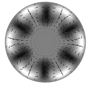
As shown in figure 11, excellent visual agreement occurs between the  $\mathcal {R}_3$-TW (where
 $\mathcal {R}_h$ represents the
 $h$-fold rotational symmetry) found by Wedin & Kerswell (Reference Wedin and Kerswell2004) and the
 $\mathcal {R}_3$-EPENS at the same Reynolds number,
 $Re_R=900$. (The Reynolds number based on the pipe diameter used in Wedin & Kerswell (Reference Wedin and Kerswell2004), Willis et al. (Reference Willis, Duguet, Omel'chenko and Wolfrum2017) and Kerswell & Tutty (Reference Kerswell and Tutty2007) has been converted to
 $Re_R$ herein.) The EPENS are shown at
 $x_R=18$ and
 $\bar {t}=0$, where
 $u_{urm,max}$ attains the largest amplitude. Remarkable agreement is observed for the streamwise vortices and the high/low-speed streaks, although the TWs are found in fully developed pipe flow, while the EPENS exist in the pipe entrance region. Both the
 $\mathcal {R}_3$-TW and
 $\mathcal {R}_3$-EPENS have three equispaced low-speed streaks (dark) located towards the centre, and three equispaced high-speed streaks (light) positioned near the wall. For both sets of nonlinear structures, streamwise vortices are located between adjacent low-speed and high-speed streaks, moving fluid towards the pipe axis in correspondence with low-speed streaks and wallward where high-speed streaks exist.
Comparison of velocity fields between the  $\mathcal {R}_3$-TW and
 $\mathcal {R}_3$-EPENS for
 $Re_R=900$. The cross-section vectors
 $\tilde {v}\boldsymbol {j}+\tilde {w}\boldsymbol {k}$ (where
 $\boldsymbol {j}$ and
 $\boldsymbol {k}$ are unit vectors in the radial and azimuthal directions) are indicated by arrows. The streamwise velocity
 $\tilde {u}$ is indicated by the shading, where light/dark colour indicates
 $\tilde {u}$ faster/slower than the laminar base-flow velocity
 $U$. The same shading is used in figures 12–14. (a) The
 $\mathcal {R}_3$-TW found by Wedin & Kerswell (Reference Wedin and Kerswell2004). (b) The
 $\mathcal {R}_3$-EPENS calculated at
 $x_R=18$, where they are most amplified, and
 $\bar {t}=0$ with
 $\epsilon =0.05$,
 $k_{x,R}=0.02$,
 $l=3$ and
 $m_0=3$.

The TWs originate mathematically from saddle–node bifurcations and are calculated using a homotopy approach. However, this numerical method does not explain the physical origin of TWs. The method to compute the EPENS instead describes the physical origin of EPENS, i.e. the EPENS arise from the algebraic growth, nonlinear interactions and streamwise stretching of realistic vortical disturbances convected by the uniform flow approaching and entering the pipe inlet. We note that other receptivity mechanisms, such as wall vibration or roughness, could also create them. Wedin & Kerswell (Reference Wedin and Kerswell2004) found that multiple solution branches coexist at higher Reynolds numbers (refer to figure 10 of Wedin & Kerswell Reference Wedin and Kerswell2004). Besides the  $\mathcal {R}_h$ solution shown in figure 11(a), which consists of
 $h$ high-speed streaks near the wall, Wedin & Kerswell (Reference Wedin and Kerswell2004) also discovered solutions with
 $2h$ near-wall high-speed streaks in other branches. Only EPENS with
 $h$ high-speed streaks are instead found in our computations.
With figure 11(b) as a reference, computations of EPENS for  $m_0=3$ are carried out for different
 $Re_R$,
 $k_{x,R}$ and
 $l$. The results are displayed in figure 12 at the locations where the EPENS are most amplified. Figure 11(a) corresponds to solution
 $a$ in figure 10 of Wedin & Kerswell (Reference Wedin and Kerswell2004), which was used for the branch continuation. This branch was traced down to
 $Re_R=785$ and up to
 $Re_R=1600$. Figures 12(a) and 12(d) show the EPENS calculated at these two Reynolds numbers. The similarities in the dominant streaks and vortices of EPENS for different
 $Re_R$ are observed. As
 $Re_R$ increases, the low-speed streaks appear slightly narrower along the azimuthal direction, and the high-speed streaks become slightly more flattened towards the wall. The close resemblance among TWs pertaining to the same branch for different
 $Re_R$ was also reported in Wedin & Kerswell (Reference Wedin and Kerswell2004). Figures 12(b) and 12(e) show that varying the frequency by one hundred times has only a minimal impact on the EPENS. The robustness of the EPENS is further confirmed in figures 12(c) and 12(f) by varying the radial modulation of the inlet perturbation flow, given by the change of the parameter
 $l$. Increasing
 $l$, indicating an inlet perturbed flow with a smaller radial length scale, has only a mild influence on the EPENS. This result proves that the EPENS are likely to be a strong attractor of the dynamical system.
Velocity fields of  $\mathcal {R}_3$-EPENS at locations where they are most amplified and
 $\bar {t}=0$ for different
 $Re_R$,
 $k_{x,R}$ and
 $l$. Unless otherwise stated, the parameters are
 $\epsilon =0.05$,
 $Re_R=900$,
 $k_{x,R}=0.02$,
 $l=3$ and
 $m_0=3$. Here, (a)
 $Re_R=785$,
 $x_R=17$, (b)
 $k_{x,R}=0.002$,
 $x_R=18$, (c)
 $l=2$,
 $x_R=22$, (d)
 $Re_R=1600$,
 $x_R=19$, (e)
 $k_{x,R}=0.2$,
 $x_R=15$, (f)
 $l=4$,
 $x_R=20$.

Except for the  $\mathcal {R}_3$ symmetry, only TWs at their saddle–node bifurcations are presented for other rotational symmetry in Wedin & Kerswell (Reference Wedin and Kerswell2004). Among these solutions,
 $\mathcal {R}_5$- and
 $\mathcal {R}_6$-TWs consist of
 $h$ high-speed streaks near the wall, while
 $\mathcal {R}_1$-,
 $\mathcal {R}_2$- and
 $\mathcal {R}_4$-TWs have
 $2h$ high-speed streaks. Remarkable agreement between TWs and EPENS is also obtained for the
 $\mathcal {R}_5$ and
 $\mathcal {R}_6$ rotational symmetries, as reported in figure 13. The EPENS with
 $h$-fold rotational symmetry observed downstream is always excited by free-stream vortical disturbances with azimuthal wavenumber
 $m_0=h$. The discovery of
 $\mathcal {R}_1$-TWs, which possess no discrete rotational symmetry, was reported in Pringle & Kerswell (Reference Pringle and Kerswell2007). These TWs are more important than the rotationally symmetric ones because the upper/lower branches correspond to much higher/lower wall-shear stress values compared to rotationally symmetric ones. Figure 14(a) shows the velocity field of an asymmetric TW of these new families. One low-speed streak is centred at half the distance between the wall and the centreline, and is surrounded by two high-speed streaks. As shown in figure 14(b), rotationally asymmetric EPENS are also found in our calculation when
 $m_0=1$. However, they consist of one wide near-wall high-speed streak flanked by two low-speed streaks, and one low-intensity high-speed streak on the opposite side of the wide high-speed streak. The cross-section velocity vector field reveals that counter-rotating streamwise vortices occur between the high-speed and low-speed streaks. Using a feedback control strategy, a new asymmetric TW was identified by Willis et al. (Reference Willis, Duguet, Omel'chenko and Wolfrum2017) (figure 14c). Good agreement is noted between the streaks of their TW and our
 $\mathcal {R}_1$-EPENS at the same Reynolds number, whereas only very weak streamwise vortices are found between the wide high-speed streak and low-speed streaks in their case.
Comparison of velocity fields between TWs and EPENS for rotational symmetries  $\mathcal {R}_5$ at
 $Re_R=1242.75$ and
 $\mathcal {R}_6$ at
 $Re_R=1434.5$. (a,c) The
 $\mathcal {R}_5$- and
 $\mathcal {R}_6$-TW found by Wedin & Kerswell (Reference Wedin and Kerswell2004) at their saddle–node bifurcations. (b,d) The
 $\mathcal {R}_5$- and
 $\mathcal {R}_6$-EPENS calculated at
 $x_R=12$ and
 $11$, where they are most amplified, and
 $\bar {t}=0$ for
 $\epsilon =0.05$,
 $k_{x,R}=0.02$,
 $l=3$ and
 $m_0=5,6$.

Comparison of velocity fields between the asymmetric TWs and  $\mathcal {R}_1$-EPENS for (a,b)
 $Re_R=1450$ and (c,d)
 $Re_R=1340$. (a,c) The asymmetric TWs found by Pringle & Kerswell (Reference Pringle and Kerswell2007) and Willis et al. (Reference Willis, Duguet, Omel'chenko and Wolfrum2017), where the white/dark coloured shading indicates
 $\tilde {u}$ faster/slower than the laminar base-flow velocity
 $U$. (b,d) The
 $\mathcal {R}_1$-EPENS calculated at
 $x_R=36$, where they are most amplified, and
 $\bar {t}=0$ with
 $\epsilon =0.05$,
 $k_{x,R}=0.02$,
 $l=3$, and
 $m_0=1$.

The comparison of streamwise velocity isosurfaces of the  $\mathcal {R}_3$-TW calculated by Kerswell & Tutty (Reference Kerswell and Tutty2007) and the
 $\mathcal {R}_3$-EPENS at
 $Re_R=1200$ is also very good, as shown in figure 15, where the light and dark shadings denote the streamwise velocity for
 $\tilde {u}=0.3U$ and
 $-0.3U$. The
 $\mathcal {R}_3$-TW is displayed versus its wavelength (the diameter of the pipe is used as a reference length), while the
 $\mathcal {R}_3$-EPENS is displayed for
 $13< x_R<17$. Along these distances, both the near-wall high-speed streaks and the low-speed streaks near the pipe core for both the TW and EPENS evolve slowly in the streamwise direction.
Comparison of streamwise velocity isosurfaces between the  $\mathcal {R}_3$-TW and
 $\mathcal {R}_3$-EPENS for
 $Re_R=1200$. The light and dark shading represents the streamwise velocity
 $\tilde {u}$ that equals
 $0.3U$ and
 $-0.3U$. (a) The
 $\mathcal {R}_3$-TW over the wavelength found by Kerswell & Tutty (Reference Kerswell and Tutty2007). (b) The
 $\mathcal {R}_3$-EPENS calculated for
 $13\ll x_R\ll 17$ and
 $\bar {t}=0$ with
 $\epsilon =0.05$,
 $k_{x,R}=0.2$,
 $l=3$ and
 $m_0=3$.

Considering the richness of the phase space, further comparison between TWs and EPENS for different parameters are warranted to fully understand their connection. One challenge in searching for an TW is the daunting numerical process required to find a good initial guess, whereas EPENS can be calculated much more rapidly using our approach. It is therefore suggested that EPENS could be used as initial guesses in the search for TWs.
3.4. Comparison with experimental data
Ricco & Alvarenga (Reference Ricco and Alvarenga2022) compared their linearised numerical results to the experimental measurements by Wygnanski & Champagne (Reference Wygnanski and Champagne1973). For both the mean and perturbation flow, excellent agreement was obtained at a low level of free-stream turbulence intensity, while a significant deviation between the linear results and the experimental data was reported for higher intensities. In figure 16, the experimental data at high turbulence intensity are compared with our nonlinear results. The turbulence intensity was measured by  $(u_{rms}/\bar {U})_{cl}$ in Wygnanski & Champagne (Reference Wygnanski and Champagne1973), where the subscript
 $cl$ refers to the value at the pipe axis. The values
 $(u_{rms}/\bar {U})_{cl}=5.8\,\%$ and
 $7.8\,\%$ in Wygnanski & Champagne (Reference Wygnanski and Champagne1973) are found to be equivalent to
 $\epsilon =0.082$ and
 $0.12$ in our calculation for the case with
 $k_{x,R}=0.118$,
 $l=2$, and
 $m_0=2$. Figure 16(a) shows the good agreement in the mean-flow velocity profiles except in the near-wall region where the numerical calculations underpredict the experimental data. Good agreement also occurs in the comparison of the perturbation-flow velocity profiles, as shown in figure 16(b). In Ricco & Alvarenga (Reference Ricco and Alvarenga2022), the velocity profile was instead predicted by the linearised boundary-region equations to be zero at the pipe axis. The finite perturbations near the pipe axis are well predicted when the nonlinear interactions (i.e.
 $r_t\,\hat {u}_{0,0}$) are taken into account. Both studies show the same trend: as the turbulent intensity increases, a larger peak is reached, and the peak position moves towards the wall. The peak of the profiles measured by Wygnanski & Champagne (Reference Wygnanski and Champagne1973) is obtained at a lower value and located closer to the wall compared to our calculations. The disagreements are likely to come from the different inflows at the pipe inlet. In experiments, the disturbances were generated by an orifice plate or a circular disk placed at the inlet, and no precise information about the resulting initial flow was given. The analytical expression (2.1) is instead used to model the vortical disturbances in our calculations. As the flow is described by an initial–boundary value problem in the pipe entrance, the inflow characteristics are crucial for an accurate prediction of the downstream development of the flow.
Comparison of (a) the mean flow and (b) the perturbation flow between the experimental measurements (circles) and present numerical results (lines) for  $Re_R=1200$ at
 $x_R = 30$. Open and solid circles: experimental data measured by Wygnanski & Champagne (Reference Wygnanski and Champagne1973) (WC73) with
 $(u_{rms}/\bar {U})_{cl}=5.8\,\%$ and
 $7.8\,\%$. Dotted and solid lines: present results with
 $\epsilon =0.082,0.12$,
 $k_{x,R}=0.118$,
 $l=2$ and
 $m_0=2$.

4. Summary and conclusions
As a step towards understanding the laminar–turbulent transition in pipe flow, we have investigated the nonlinear evolution of free-stream vortical disturbances entrained in the entrance region of a circular pipe by using a high Reynolds number asymptotic approach. The oncoming disturbances are modelled by a pair of vortical modes with the same frequency but opposite azimuthal wavenumber. A long-wavelength hypothesis is utilised. This hypothesis is inspired by the experimental finding that streamwise-elongated streaks induced by free-stream disturbances in boundary layers amplify significantly (Matsubara & Alfredsson Reference Matsubara and Alfredsson2001). The disturbance amplitude is assumed to be intense enough for nonlinear interactions to occur. The present study can therefore be viewed as an extension of Ricco & Alvarenga (Reference Ricco and Alvarenga2022) to the nonlinear case.
The resultant nonlinear system is solved numerically by a marching procedure in the streamwise direction. A parametric study reveals the stabilising effect of nonlinearity on the intense algebraic disturbance growth near the pipe inlet. The linear theory thus overpredicts the nonlinear disturbance intensity. The effect of the Reynolds number, the streamwise and azimuthal wavelengths, and the radial length scale of the inlet disturbance on the nonlinear evolution of the disturbances is investigated. The mean-flow distortion  $\hat {u}_{0,0}$ grows significantly shortly downstream of the pipe inlet, being negative in the pipe core and positive near the wall, indicating an increase of wall-shear stress.
We report the formation, amplification and attenuation of rotationally symmetric elongated pipe-entrance nonlinear structures (EPENS). The distinct features of  $\mathcal {R}_h$-EPENS (
 $h>1$) are equispaced
 $h$ high-speed streaks around the pipe wall, and
 $h$ low-speed streaks in the pipe core. A remarkable resemblance between these structures and nonlinear travelling waves (TWs) occurring in fully developed pipe flow is noted for
 $m_0=3,5,6$. Rotationally asymmetric EPENS are discovered for
 $m_0=1$. They also agree well with asymmetric TWs for
 $m_0=1$. These similarities may shed light on the physical origin of nonlinear TWs. The robustness of the EPENS in response to changes of different inlet flow conditions is demonstrated, indicating that the EPENS are likely to be a strong attractor of the dynamical system. We also suggest the potential use of EPENS as an initial guess in the numerical search for the nonlinear TWs. More investigations are necessary to clarify the connection between the EPENS and the TWs.
With the inclusion of nonlinear effects, good agreement between our calculations and the experimental measurements of Wygnanski & Champagne (Reference Wygnanski and Champagne1973) is obtained for both the mean flow and the perturbation flow. Further improvement may be gained by using a continuous spectrum of free-stream disturbances as oncoming disturbances. Performing a secondary instability analysis of the EPENS is also of interest. The EPENS attenuate downstream in our calculation, but they may persist when the growth of small-amplitude secondary disturbances is taken into account.
It is our hope that the theoretical work presented herein will motivate more direct numerical simulations and experimental investigations in the entrance region of pipe flow.
Acknowledgements
The authors would like to thank the Faculty of Engineering of the University of Sheffield for funding this research. The authors are also indebted to Dr E. Marensi for her insightful comments.
Funding
This work was funded by a Faculty of Engineering University Research Scholarship from the University of Sheffield.
Declaration of interests
The authors report no conflict of interest.
Appendix A. Conservation of the mass flow rate
At each instant in time and at each streamwise location, the mass flow rate is conserved. Since the flow is incompressible, this condition translates to the conservation of the bulk velocity, i.e. the streamwise velocity averaged on the cross-section of the pipe is equal to the oncoming velocity  $U_\infty ^*$:
 \begin{equation} \frac{1}{{\rm \pi} R^2} \int_0^{2 {\rm \pi}} \int_0^R (U + r_t \bar{u} ) r \,\mathrm{d}r\, \mathrm{d}\theta = 1. \end{equation}
Substituting (2.7) into (A1), equation (2.11) is obtained for the laminar base flow, and
 \begin{equation} \sum_{m,n={-}\infty}^{\infty} \int_0^{2 {\rm \pi}} \int_0^R \hat{u}_{m,n}\, {\rm e}^{{\rm i}m\theta+{\rm i}n\bar{t}} r \,\mathrm{d}r \,\mathrm{d}\theta = 0. \end{equation}
By using the orthogonality property of the Fourier series, equation (2.20) is obtained, which is the condition needed to solve the system because the pressure  $\varGamma _{0, n}$ is an additional unknown.
Appendix B. Coefficients of equation (2.27)
The expressions of  $\{\hat {V}, \hat {V}_r, \hat {V}_x,\ldots,\hat {U}_{xrr}\}$ in (2.27) are
 \begin{gather} \hat{V} = \left(1-\frac{1}{m^2}\right)\left({\rm i}n + \frac{\partial V}{\partial r} + \frac{m^2-1}{\mathcal{F} r^2}\right) + \frac{2r}{m^2}\,\frac{\partial^2 U}{\partial\bar{x}\,\partial r} + \frac{r^2}{m^2}\,\frac{\partial^3 U}{\partial\bar{x}\,\partial r^2}, \end{gather}
 \begin{gather}\hat{V}_r = \left[\left(1-\frac{4}{m^2}\right)V-\frac{3r}{m^2}\left({\rm i}n + \frac{\partial V}{\partial r}\right)-\left(2+\frac{1}{ m^2}\right)\frac{1}{\mathcal{F}r}\right] + \frac{r^2}{m^2}\,\frac{\partial^2 U}{\partial\bar{x}\,\partial r}, \end{gather}
 \begin{gather}\hat{V}_x = \left(1-\frac{1}{m^2}\right)U+\frac{r}{m^2}\left(\frac{\partial U}{\partial r} + r\,\frac{\partial^2 U}{\partial r^2}\right), \end{gather}
 \begin{gather}\hat{V}_{rr} ={-}\left[\frac{r}{m^2}\left({\rm i}nr+5V+r\,\frac{\partial V}{\partial r}\right) + \left(2-\frac{5}{m^2}\right)\frac{1}{\mathcal{F}}\right], \end{gather}
 \begin{gather}\hat{V}_{xr} ={-}\frac{3Ur}{m^2}, \end{gather}
 \begin{gather}\hat{V}_{rrr} ={-}\frac{r}{m^2}\left(rV-\frac{6}{\mathcal{F}}\right), \end{gather}
 \begin{gather}\hat{V}_{xrr} ={-}\frac{r^2U}{m^2}, \end{gather}
 \begin{gather}\hat{V}_{rrrr} = \frac{r^2}{m^2\mathcal{F}}, \end{gather}
 \begin{gather}\hat{U} = \frac{\partial V}{\partial \bar{x}} + \frac{2r}{m^2}\,\frac{\partial^2 U}{\partial \bar{x}^2} + \frac{r^2}{m^2}\,\frac{\partial^3 U}{\partial \bar{x}^2\,\partial r}, \end{gather}
 \begin{gather}\hat{U}_r = \frac{r}{m^2}\,\frac{\partial V}{\partial \bar{x}}, \end{gather}
 \begin{gather}\hat{U}_x ={-} \frac{2}{\mathcal{F} r} + \frac{6r}{m^2}\,\frac{\partial U}{\partial \bar{x}} + \frac{2r^2}{m^2}\,\frac{\partial^2 U}{\partial \bar{x}\,\partial r}, \end{gather}
 \begin{gather}\hat{U}_{rr} = \frac{r^2}{m^2}\,\frac{\partial V}{\partial \bar{x}}, \end{gather}
 \begin{gather}\hat{U}_{xr} = \frac{2}{m^2}\left(\frac{1}{\mathcal{F}}-2Vr-r^2\,\frac{\partial V}{\partial r}\right), \end{gather}
 \begin{gather}\hat{U}_{xrr} = \frac{2r}{m^2\mathcal{F}}. \end{gather}
Appendix C. Modified block tridiagonal matrix algorithm
A modified block tridiagonal matrix algorithm is devised for solving the discretised version of system (2.30)–(2.32) together with the discretised (2.20) for  $m=0$,
 \begin{equation} \boldsymbol{A\delta}=\boldsymbol{b}. \end{equation}
In expanded form, the system (C1) is
 \begin{equation} \begin{bmatrix} A_1 & C_1 & & & & & & E_1\\ B_2 & A_2 & C_2 & & & & & E_2\\ & \cdots & \cdots & \cdots & & & & \cdots\\ & & B_j & A_j & C_j & & & E_j\\ & & & \cdots & \cdots & \cdots & & \cdots\\ & & & & B_{J-3} & A_{J-3} & C_{J-3} & E_{J-3}\\ & & & & & B_{J-2} & A_{J-2} & E_{J-2}\\ D_1 & D_2 & D_3 & & \cdots & & D_{J-2} & 0 \end{bmatrix} \begin{bmatrix} \delta_1\\ \delta_2\\ \cdots\\ \delta_j\\ \cdots\\ \delta_{J-3}\\ \delta_{J-2} \\ \varPi \end{bmatrix} = \begin{bmatrix} b_1\\ b_2\\ \cdots\\ b_j\\ \cdots\\ b_{J-3}\\ b_{J-2} \\ 0 \end{bmatrix},\end{equation}
where  $A_j$,
 $B_j$ and
 $C_j$ are
 $3 \times 3$ matrices,
 $E_j$,
 $\delta _j$ and
 $b_j$ are
 $3 \times 1$ matrices,
 $D_j$ is a
 $1 \times 3$ matrix, and
 $\varPi$ is a scalar. In (C2), row
 $j$ for
 $2\leq j\leq J-3$ represents the discretised equations (2.30)–(2.32) at the interior nodes, while rows 1 and
 $J-2$ refer to the equations at the boundaries. The last row is the discretised integral (2.20).
First, we add any two decoupled equations to the system in order to add two rows at the bottom of matrix  $\boldsymbol {A}$ and two columns on the right of matrix
 $\boldsymbol {A}$. This step makes
 $D_j$ and
 $E_j$
 $3 \times 3$ matrices, and creates two
 $3 \times 1$ matrices,
 $\delta _{J-1}$ and
 $b_{J-1}$, at the bottom of
 $\boldsymbol {\delta }$ and
 $\boldsymbol {b}$, which is necessary in order to render the system suitable for the block elimination. The matrices
 $D_j$ and
 $E_j$ are renamed
 $\mathcal {D}_j$ and
 $\mathcal {E}_j$. The system (C2) becomes
 \begin{equation} \begin{bmatrix} A_1 & C_1 & & & & & & \mathcal{E}_1\\ B_2 & A_2 & C_2 & & & & & \mathcal{E}_2\\ & \cdots & \cdots & \cdots & & & & \cdots\\ & & B_j & A_j & C_j & & & \mathcal{E}_j\\ & & & \cdots & \cdots & \cdots & & \cdots\\ & & & & B_{J-3} & A_{J-3} & C_{J-3} & \mathcal{E}_{J-3}\\ & & & & & B_{J-2} & A_{J-2} & \mathcal{E}_{J-2}\\ \mathcal{D}_1 & \mathcal{D}_2 & \mathcal{D}_3 & & \cdots & & \mathcal{D}_{J-2} & \mathcal{E}_{J-1} \end{bmatrix} \begin{bmatrix} \delta_1\\ \delta_2\\ \cdots\\ \delta_j\\ \cdots\\ \delta_{J-3}\\ \delta_{J-2} \\ \delta_{J-1} \end{bmatrix} = \begin{bmatrix} b_1\\ b_2\\ \cdots\\ b_j\\ \cdots\\ b_{J-3}\\ b_{J-2} \\ b_{J-1} \end{bmatrix}.\end{equation}
The standard block tridiagonal matrix algorithm described in Cebeci (Reference Cebeci2002) is modified to solve (C3), which also consists of the forward sweep and backward substitution. However, in each forward sweep, one more step needs to be performed to eliminate  $\mathcal {D}_j$, which leads to
 \begin{equation} \begin{bmatrix} I & C_1' & & & & & & \mathcal{E}_1'\\ & I & C_2' & & & & & \mathcal{E}_2' \\ & & \cdots & \cdots & & & & \cdots\\ & & & I & C_j' & & & \mathcal{E}_j'\\ & & & & \cdots & \cdots & & \cdots\\ & & & & & I & C_{J-3}' & \mathcal{E}_{J-3}'\\ & & & & & & I & \mathcal{E}_{J-2}'\\ & & & & & & & \mathcal{E}_{J-1}' \end{bmatrix} \begin{bmatrix} \delta_1\\ \delta_2\\ \cdots\\ \delta_j\\ \cdots\\ \delta_{J-3}\\ \delta_{J-2} \\ \delta_{J-1} \end{bmatrix} = \begin{bmatrix} b_1'\\ b_2'\\ \cdots\\ b_j'\\ \cdots\\ b_{J-3}'\\ b_{J-2}' \\ b_{J-1}' \end{bmatrix}, \end{equation}
where the prime denotes the new coefficients. The solution is then obtained by backward substitution:
 \begin{equation} \left. \begin{array}{c} \delta_{J-1} = \mathcal{E}_{J-1}'^{{-}1}b_{J-1}',\\ \delta_{J-2} = b_{J-2}' - \mathcal{E}_{J-2}'\delta_{J-1},\\ \delta_i = b_i' - C_i'\delta_{i+1} - \mathcal{E}_i'\delta_{J-1}, \quad i=J-3,J-4,\ldots,1. \end{array} \right\} \end{equation}



