


A central role of government is the provision of public goods to its citizenry. Most public goods provided by governments are durable, and hence dynamic in nature. It takes time to accumulate them, and they depreciate slowly, projecting benefits for many years. Prominent examples are national defense, environmental protection, and public infrastructure. Although a large literature has studied public good provision and public policy formation by governments or legislatures in static models, both theoretically and empirically, much less is known about the dynamics of public investments. Two political economy questions immediately come to mind. First, can we say anything about the efficiency of dynamic public investment by legislatures or governing bodies operating under democratic rules? Second, to what extent does the efficiency depend on the specific voting rules under which these governing bodies operate? Again, little is known about these effects, except for highly specialized static environments, where only a single decision is taken (for example, Baron and Ferejohn Reference Baron and Ferejohn1989, Volden and Wiseman 2005).
The debate on the policy consequences of different voting rules has important practical implications, because we observe a large variety of voting rules in the real world. In a parliamentary assembly, motions on the floor are usually passed by a simple majority. However, a broader consent is required in many other contexts, and examples are widespread across different systems of government. In the European Union's Council of Ministers, some proposals require only a simple majority, some a supermajority, and some unanimous consent. As of the writing of this article, explicit supermajorities are required in most countries to pass constitutional reform, and 16 U.S. states (Arizona, Arkansas, California, Colorado, Delaware, Florida, Kentucky, Louisiana, Michigan, Mississippi, Missouri, Nevada, Oklahoma, Oregon, South Dakota, Washington) require a two-thirds supermajority legislative vote to increase taxes. There is a large literature studying the comparative performance of different voting rules going back to Rousseau ([1762] Reference Rousseau1988), Condorcet (Reference Condorcet1785), Wicksell ([1896] Reference Wicksell and Buchanan1967), Buchanan and Tullock (Reference Buchanan and Tullock1962), and more recently Austen-Smith and Banks (Reference Austen-Smith and Banks1996) and Cox (Reference Cox1987). In contrast to our approach, those works focus on static settings and typically deal with purely distributive politics or reforms with unknown winners, rather than with investment in a public project.
In this article, we make a first attempt to answer the questions mentioned earlier by proposing a new theoretical framework for studying the political economy of dynamic public good provision. We analyze a legislative bargaining model under alternative voting rules and examine its predictions in a laboratory experiment. The basic environment we study consists of many citizens who live in n equal-sized districts and can invest resources over time to accumulate a stock of durable public good (roads, bridges, sewers, etc.). An investment policy is taken each period by a central governing body, the legislature, composed of a single representative from each district, and operating under a procedure consisting of an agenda-setting stage and a voting rule. In each period, the legislature has the power to allocate a fixed budget of resources between investment in the public good (whose utility is enjoyed by all citizens of all districts) and targeted transfers to each district.Footnote 1 Representatives bargain in the legislature over the budget allocation. We characterize the trajectory of public policies that would result from a symmetric Markov perfect equilibrium for any q rule adopted by the legislature, where a q rule requires q out of n yes votes for passage of the policy for the current period. We compare these equilibrium trajectories with the optimal public policy (i.e., the policy that maximizes the welfare of the citizens).
The equilibrium generates clear predictions about how the dynamics of investment are affected by the voting rule the legislature uses to make its decisions. The model implies that a stricter requirement for passage (i.e., higher q) will generate a higher level of investment and a higher steady state of the public good. The intuition for this is twofold: (1) a higher q forces proposers to internalize a larger share of the public good, and (2) stricter requirements for passage also mitigate worries about future proposers’ incentives to plunder the current public good investments. The former effect is similar to the familiar static free rider problem, whereas the latter effect is entirely dynamic and relates, for example, to models in which politicians on the way out of power may run up debt in order to tie the hands of their successors.Footnote 2 For any voting rule, investment should continue until a steady state is reached, and the equilibrium steady states are monotonically increasing in q. For any q rule except unanimity, this steady state is lower than in the optimal solution. Furthermore, for any voting rule including unanimity, the speed of investment along the transition path to the steady state is slower than in the optimal solution, because proposers with agenda control have an incentive to skim off resources along the way.
Our finding that a higher majority requirement leads to higher long-run public investment and hence more dynamically efficient public policy provides a formal rationale for Wicksell ([1896] Reference Wicksell and Buchanan1967), who, more than a century ago, advocated unanimity as the only rule guaranteeing Pareto improvements. However, in our dynamic setting, the impact of the voting rule on the economic outcomes is more complex (and perhaps surprising): Even with unanimity, the accumulation path is predicted to be inefficiently slow, and when the marginal value of investment is high, a higher majority rule increases, rather than reduces, the amount of rents an agenda-setting proposer can guarantee to the district he represents.
We examine the predictions of the theory by conducting a carefully designed series of controlled laboratory experiments. In the experiments, we focus on three alternative voting rules: a dictatorship rule (D), a simple majority rule (M), and a unanimity rule (U). There are several reasons for examining the theory with data from controlled experiments. First, some kind of data are needed to discipline the theory. It is important to identify whether the theory is at all reasonable from a behavioral or empirical standpoint. Second, if one is going to take the model to data, there are clear identification advantages for experimental studies when studying a highly structured dynamic environment such as the one in this article. In our model, strategic behavior can be clearly identified only if there is a precise measurement of certain state variables as well as the actions available to the players, and for this purpose, data from laboratory experiments that control key variables in observable ways have some obvious advantages over field data. The control of laboratory experiments allows us to directly test the main comparative static implication of the theory: Do higher q rules lead to more efficient investment paths?
A third motivation for pursuing the experiments is that the predictions and assumptions of the model seem unintuitive and in many ways implausible. The legislators in the model are assumed to be completely rational and selfish, with rational expectations and perfect foresight about the entire infinite equilibrium path of public policies. Any behavioral limitations, bounded rationality, or other-regarding preferences are completely assumed away, and in principle the presence of these factors could drastically change the predictions of the model. Indeed, the modeling assumptions that people are perfectly rational, purely selfish, and have perfect foresight are abstractions, and there is ample reason to be skeptical of the predictions that come out of such models. This leads to the second basic question we ask: Are the predictions of the model robust to behavioral factors and limitations on perfect rationality that we know exist but are assumed away in the model?
Finally, it is important to note that our model's predictions only apply to a very small subset of the huge set of subgame perfect equilibria in the infinite game. In particular, there generally exist non-Markov equilibria that lead to efficient investment paths independently of the q rule. Such equilibria closely resemble cooperative equilibria in repeated games, such at the prisoner's dilemma. We know from experiments that groups are highly successful at achieving efficient outcomes in repeated prisoner's dilemma and similar games (Dal Bo Reference Dal Bo2005). Hence the third basic question: Can the inefficiencies be overcome? Do efficient investment paths emerge in these legislative bargaining games, possibly due to the repeated game effects created by the dynamic environment?
The effect of q on the efficiency of public policy is confirmed by the experimental data. A higher q rule leads to better public policies in the form of significantly greater public good investment. Second, in addition to these qualitative findings, the public good levels are also quantitatively close to the predictions of the Markov perfect equilibrium. Also consistent with this equilibrium, players’ choices reflect non-myopic decision making: The theoretical expected continuation value functions are the most important significant variables explaining voting behavior. Thus, the behavior in these complicated environments appears to be largely robust to factors outside the model, such as bounded rationality and other-regarding preferences. Of course the data are not a perfect match to the theory. We observe some differences between the finer details of the theoretical predictions and the data. The clearest such deviation is a statistically significant overinvestment in the early rounds under all voting rules. This phenomenon is reminiscent of the finding in experiments on static public good provision (by a centralized legislature or in a voluntary provision setting), but it is more complex in our dynamic setting: while we observe a large initial overinvestment in the early rounds, this initial overinvestment is mostly “undone” in later rounds, as it is usually followed by significant disinvestment (in D and M) or lack of further investment (in U) approaching the equilibrium steady state.
We view these experimental findings as an encouraging initial check on the validity of a few general principles that are implied by our model, which have the potential to be important factors in legislative decision making and can be easily isolated in a laboratory experiment. The actual political institutions that motivate our study (parliaments, assemblies, legislatures, etc.) are obviously far more complex than the simple environments we study in the experiment, which, by design, mirrors the starkness of the model. With this in mind, it is worth noting that there do exist historical data that bear on some of the hypotheses generated by our theoretical model. For example, Rauch's (Reference Rauch1995) study of municipal reforms during the U. S. Progressive era suggests that reforms that lengthened the time horizon of municipal governments led to an increase in new investment in public infrastructure. There may also be questions about robustness to other subject pools, but in principle these latter kinds of external validity issues are relatively straightforward (but very costly) to resolve, by replication using subjects with different characteristics or expertise, such as professional politicians, or by using alternative procedures and settings tailored to the richer details of specific institutions.
RELATED LITERATURE
This article contributes primarily to the literature on the impact of institutions on the dynamics of public good provision, which includes the important special case of common-pool resources management. Along these lines, Walker et al. (Reference Walker, Gardner, Herr and Ostrom2000), Ostrom (Reference Ostrom1990), and Ostrom, Gardner, and Walker (Reference Ostrom, Gardner and Walker1994) examine both theoretically and empirically how communication, voting rules, and other institutions for collective decision making affect the outcome of commons dilemma games. Olson (Reference Olson1993) and McGuire and Olson (Reference McGuire and Olson1996) compare the negative externalities that a democratic majority and an autocrat might impose on society.
Related to the theoretical approach of this article is a series of recent papers on dynamic political economy. Battaglini and Coate (Reference Battaglini and Coate2006) study public good accumulation in a different political-economic environment and consider a different bargaining protocol. Their results are different from ours in several ways: The budget in each period is endogenously determined, there is distortionary taxation, and preferences are stochastic.Footnote 3 Battaglini, Nunnari, and Palfrey (Reference Battaglini, Nunnari and Palfrey2012) explore the question of dynamic public good investment in a decentralized game without voting. Also related, but less directly, is the earlier research by Boylan, Ledyard, and McKelvey (Reference Boylan, Ledyard and McKelvey1996) and Boylan and McKelvey (Reference Boylan and McKelvey1995) that studies a one-sector model of economic growth in which decisions about investment are made by a competitive political process. That research focuses on the effect of commitment on investment cycles. Harstad (Reference Harstad2005) considers a club that decides by majority rule whether to undertake a joint public project. He studies how the size of this majority (that is, the q-rule adopted) affects the incentives of each member to invest in order to increase his or her valuation of the project.
This article is also the first experimental study of the dynamic accumulation process of a durable public good by a legislature. Our findings thus extend the recent experimental literature on legislative bargaining models to dynamic settings. McKelvey (Reference McKelvey and Palfrey1991) is the first experimental study of legislative bargaining models à la Baron and Ferejohn (Reference Baron and Ferejohn1989). Diermeier and Gailmard (Reference Diermeier and Gailmard2006), Diermeier and Morton (Reference Diermeier, Morton, Austen-Smith and Duggan2006), Frechette, Kagel, and Lehrer (Reference Frechette, Kagel and Lehrer2003), and others have also reported laboratory experimental studies of legislative bargaining, but only in a static setting with purely distributive policies. Recently, Frechette, Kagel, and Morelli (Reference Frechette, Kagel and Morelli2012) have extended the experimental analysis to policy spaces with public goods using a model based on Volden and Wiseman (Reference Volden and Wiseman2007). All of these works, however, limit the analysis to static environments in which only a single policy outcome is decided. Battaglini and Palfrey (Reference Battaglini and Palfrey2012) study a simple dynamic model of legislative bargaining, but limit the analysis to purely distributive policies in which public goods cannot be accumulated and redistribution across periods is not possible.
Our work is also related, though somewhat less so, to the vast experimental literature on the voluntary provision of public goods, with many of the early contributions surveyed in Choi, Gale, and Kariv (Reference Choi, Gale and Kariv2008), Choi et al. (Reference Choi, Gale, Kariv and Palfrey2011), Duffy, Ochse, and Vesterlund (Reference Duffy, Ochs and Vesterlund2007), Harrison and Hirschleifer (Reference Harrison and Hirshleifer1989), and Ledyard (Reference Ledyard, Kagel and Roth1997) specifically examine sequential contribution mechanisms for provision of a nondurable public good. In these studies, payoffs are one-shot and depend only on the sum of investments over the entire horizon. A few papers explore the effect of institutions (e.g., Smith Reference Smith1977 and Ferejohn et al. Reference Ferejohn, Forsythe, Noll, Palfrey and Smith1982), but most work in this area has focused on other questions, including the role of communication, experience, other-regarding preferences, and other behavioral factors.
MODEL
Consider an economy in which a continuum of infinitely lived citizens live in n districts and each district contains a mass one of citizens. There are two goods: a private good x and a public good g. An allocation is an infinite non-negative sequence of public policies, z = (x ∞, g ∞) where x ∞ = (x 11, . . ., xn 1, . . ., x 1t, . . ., xnt, . . .) and g ∞ = (g 1, . . ., gt, . . .). We refer to zt = (xt, gt) as the public policy in period t. The utility Uj of a representative citizen in district j is a function of zj = (xj ∞, g ∞), where xj ∞ = (xj 1, . . ., xjt, . . .). We assume that Uj can be written as

where u(·) is continuously twice differentiable, strictly increasing, and strictly concave on [0, ∞), with lim g→0+u′(g) = ∞ and limg→∞+u′(g) = 0. The future is discounted at a rate δ.
There is a linear technology by which the private good can be used to produce public good, with a marginal rate of transformation p equal to 1. The private consumption good is nondurable, whereas the public good is durable. Thus, if the level of public good at time t − 1 is g t − 1 and the investment in the public good is It, then the level of public good at time t will be

Because all citizens in district j are identical, we refer collectively to the “behavior of a district” as described by the behavior of a representative citizen j. Henceforth we simply refer to district j. In period t, the economy is endowed with Wt units of private good, where Wt = W ∀t. The initial stock of public good is g 0 ≥ 0, exogenously given.
The public policy in period t is required to satisfy three feasibility conditions:

The first two conditions guarantee that allocations are non-negative. We assume that public investment can be scaled back in the future at no cost. The third condition requires that the current budget is balanced. These conditions can be rewritten slightly. If we denote y ≡ gt = g t − 1 + It as the new level of public good after an investment It when the last period's level of the public good is g t − 1, then the public policy in period t can be represented by a vector (y, x 1t, . . ., xnt). Dropping the t subscripts and substituting y, the budget balance constraint It + ∑j = 1nx tj ≤ Wt can be rewritten as

recalling that we use y to denote the post-investment level of public good attained in period t, and g for the pre-investment level of public good inherited from period t − 1. The one-shot utility to district j from this public policy, (y, x 1, . . ., xn), is Uj = xj + u(y).
Our interest in this article is to analyze the performance of a class of political procedures in building public infrastructure (i.e., generating a feasible sequence of public policies, z). We consider a legislature where representatives of each district bargain with each other to decide how to divide the current period's societal endowment between public investment and private transfers to each district. We consider procedures that are time independent and have no commitment. That is, the voting procedures are the same in every period, and the outcome of the procedure is a public policy for only the current period. The level of the state variable g, however, creates a dynamic linkage across policy-making periods. In such procedures, we characterize the outcomes associated with symmetric Markov perfect equilibria.
OPTIMAL PUBLIC POLICY
As a benchmark with which to compare the equilibrium allocations by a legislature, we first analyze the sequence of public policies that maximizes the sum of utilities of the districts. This is the optimal public policy. This optimization problem has a recursive representation in which g is the state variable, and the value function vO(g) can be represented as

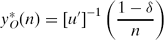
By standard methods (see Stokey, Lucas, and Prescott Reference Stokey, Lucas and Prescott1989) we can show that a continuous, strictly concave and differentiable vO(g) that satisfies (1) exists and is unique. The optimal policies have an intuitive characterization.Footnote 4 When the accumulated level of public good is low, the marginal benefit of investing in g is high, and it is efficient to invest as much as possible: In this case yO(g) = W + g and ∑nj = 1xi = 0. When g is high, it is efficient to reach the level of public good y*O(n) that solves the unconstrained optimization problem in (1): that is, nu′(y*O(n)) + δv′O(y*O(n)) = 1, as shown in the Appendix. This implies:
For gO ≥ y*O(n) − W, therefore, investment will stop, yO(gO) = y*O(n), and without loss of generality, xi = xo = (W + g − y)/n.Footnote 5 The policy and the investment functions, therefore, have the following simple structure:


This investment function implies that, in the optimal solution, the stock of the public good converges to a unique steady state, yoO = y*O(n). In yoO, the per agent level of private consumption is positive: x* = W/n > 0. Figure 1 provides a representation of the optimal investment path.
The Optimal Public Policy

POLITICAL EQUILIBRIUM
We now consider a legislature, composed of a representative from each district, that bargains over the allocation of the economy-wide resources among private goods and public good investment. In this mechanism, in each period, the legislature decides on a level of investment in the public good. The legislative policy also includes an allocation of the budgetary surplus (endowment minus investment) to the districts, which is non-negative for all districts, but not necessarily uniform. Investment can be negative, but the amount of negative investment cannot exceed the current stock of public good. Thus, we can represent a policy by the legislature at time t, by a public policy (x 1t, . . ., xnt, yt) that satisfies the same feasibility constraints as in the previous section. The bargaining protocol with which a public policy is chosen in a legislature is as follows. At the beginning of each period an agent is chosen by nature to propose a policy (x 1, . . ., xn, y). Each legislator has the same probability to be recognized as proposer. If at least q∈{1, 2, . . ., n} legislators vote in favor of the proposal, it passes and it is implemented. The legislature then adjourns and meets in the following period with a new level of public good y. If instead the policy does not receive a qualified majority, then the status quo policy is implemented. We assume that the status quo is zero investment in the public good and xj = W/n for all j. The legislature, moreover, adjourns and meets in the following period with a new level of public good g.
To characterize behavior when policies are chosen by a legislature we look for a symmetric Markov perfect equilibrium. In this type of equilibrium, equilibrium strategies depend only on payoff-relevant information, and all representatives use the same strategy. Therefore, in a symmetric Markov perfect equilibrium, any representative selected to propose at some time t uses the same strategy, and this depends only on the current stock of public good (g). Similarly, the probability a legislator votes for a proposal depends only on the proposal itself and the state g. As is standard in the theory of legislative voting, we focus on weakly stage-undominated strategies, which implies that legislators vote for a proposal if and only if their expected utility (current payoff plus discounted continuation value) from the status quo is not greater than their expected utility from the proposal. Without loss of generality, we focus on an equilibrium in which proposals are accepted with probability one on the equilibrium path.
It is easy to verify that, in a symmetric Markov perfect equilibrium, a proposer would either make no monetary transfer to the other districts or would make a transfer to exactly q − 1 legislators. An equilibrium can therefore be described by a collection of functions {yL(g), sL(g)} that specify the choice made by the proposer in a period in which the state is g. Here yL(g) is the proposed new level of public good, and sL(g) is a transfer offered to the q − 1 other districts.Footnote 6 The proposer's district receives the surplus revenues xL(g) = W − yL(g) + g − (q − 1)sL(g). Associated with any symmetric Markov perfect equilibrium in the L game is a value function vL(g) that specifies the expected continuation payoff of a legislator when the state is g before the proposer is selected.
Contrary to the case of the previous section, the policy is now chosen by a self-interested proposer who maximizes the utility of his own district. Given vL, the proposer's problem is
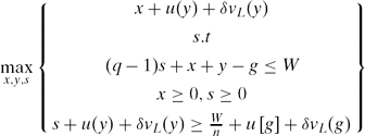
where x is the transfer to the proposer. This problem is similar to the efficient problem (1): The first inequality is the budget balance constraint, and the following two inequalities are the feasibility constraints.Footnote 7 The last inequality is, however, new: It is the incentive compatibility constraint that needs to be satisfied if a proposal is to be accepted by q − 1 other districts.
The solution to (5) is complicated by the fact that the set of binding constraints is state dependent and the value function is not typically concave in g. Despite this, the next result shows a sufficient condition for the existence of a Markov perfect equilibrium. We say that an equilibrium is regular if the associated value function is continuous, nondecreasing, and almost everywhere differentiable, and leads to a strictly concave objective function in (5). We have the following proposition:
Proposition 1. There are a =  < 1 and a
 > 0 such that for all δ > , and all W > a regular Markov perfect equilibrium exists in which the public good level is given by
![\begin{equation}
y_{L}(g) = \left\lbrace \begin{array}{c@{}c}y_{1}^{\ast } & g\le g_{1}(y_{1}^{\ast }) \\
[5pt] \widetilde{y}(g) & g\in \left( g_{1}(y_{1}^{\ast }),g_{2}(y_{L}^{\ast }) \right] \\
[5pt] y_{L}^{\ast } & else\\
\end{array} \right.
\end{equation}](https://static.cambridge.org/binary/version/id/urn:cambridge.org:id:binary:20160312035210217-0934:S0003055412000160_eqn6.gif?pub-status=live)
where y*1and y*Lare constants with y*L > y*1; g 1(y*1), g 2(y*L) are functions, respectively, of y*1and y*L; and  (g) is an increasing function of g.Footnote 8
There is an intuitive explanation for the shape of the policy function (6). For g≤g 1(y*1) the proposer acts as if the other districts did not exist, diverting resources only toward his own district and choosing the investment without internalizing the other districts’ welfare. This implies that the proposer can choose y*1 where

The other districts accept this policy because the investment y*1, is sufficiently high to make this policy better than the status quo. When g ≥ g 1(y*1), the proposer cannot afford to ignore the other districts. He first finds it optimal to “buy” their approval by increasing g and investing (g) > y 1* (in the interval (g 1(y*1), g 2(y*L)]): (g) is chosen large enough to satisfy the incentive compatibility constraint as an equality. For g > g 2(y*L), however, the proposer finds it optimal to offer positive transfers of the consumption good to a minimal winning coalition of districts, and to invest y*L. In choosing y now the proposer must internalize the utility of q legislators, so

It is interesting to note that when the proposer's strategy is constant (at y*1 or at y*L) we have a dynamic free rider problem: An increase in investment above, say, y*L, at t would induce a proportional reduction in investment at t + 1 and so discourage public good accumulation. This is key to understanding underinvestment in the steady state. When yL(g) = (g) the dynamic free rider problem is mitigated because an increase in g induces an increase in (g). This occurs because the increase in g makes the incentive constraint at t + 1 more binding, so it forces the proposer in the following period to increase the investment in the public good.
The next result guarantees that the equilibrium outcome is unique:
Proposition 2. For δ > , and W > as defined in Proposition 1, the legislative game has a unique regular equilibrium steady state,  .
Figure 2 provides a representation of the equilibrium. The first panel of Figure 2 represents the investment function IL(g):
![\begin{equation}
I_{L}(g) = \left\lbrace \begin{array}{c@{\quad }c}y_{1}^{\ast }-g & g\le g_{1} \\
[5pt] \widetilde{y}(g)-g & g\in \left( g_{1},g_{2}\right] \\
[5pt] y_{L}^{\ast }-g & else \end{array} \right.
\end{equation}](https://static.cambridge.org/binary/version/id/urn:cambridge.org:id:binary:20160312035210217-0934:S0003055412000160_eqn9.gif?pub-status=live)
(where for simplicity g 1 is the equilibrium value g 1(y*1), and similarly for g 2). It is interesting to note that while in the optimal solution IO(g) is a monotonically (weakly) decreasing function, in the political equilibrium IL(g) is not monotonic (compare (9) with the investment in the optimal solution, i.e. IO(g) = min {W, y*O − g}). The non-monotonicity of the investment function is a consequence of the fact that the incentive compatibility constraint is not always binding and the value of the status quo is endogenous. The second panel of Figure 2 shows the equilibrium proposed level of the public good as a function of the state, yL(g). This curve fully describes the dynamics of public good provision and the steady state. The steady state level of public good y*L corresponds to the point where the 45° line intersects the investment curve.
Legislative Game Equilibrium, I(g) and y(g)

How does the accumulation of public good in the political equilibrium compare to the optimal solution? Do legislatures provide durable public goods efficiently? And how does this depend on the voting rule adopted? The next result addresses these questions.
Proposition 3. (a). 0 < y*L(1, n) < y L*(2, n)< . . . < y*L(n,n) = y O*(n); (b) IL(g; q, n) < IO(g; n) ∀ n > 1, ∀ q = 1, . . ., n, and ∀ g≤ y*O(n).
Proposition 3(a) states that the equilibrium steady state of the legislative game is less than the steady state of the optimal solution for any q-voting rule but unanimity, and it is equal to the steady state of the optimal solution for q = n (with efficiency monotonically increasing in q). Proposition 3(b) states that for any voting rule, including unanimity, the accumulation of the public good that leads to the steady state is inefficiently slow. This result arises because, in any legislative game (including unanimity), the proposer finds it profitable to divert some resources toward private transfers to his own district and to q − 1 other districts (as discussed earlier).Footnote 9
Example.Let the utility function for the public good be the power function,  . The unique long-run steady state in the optimal solution is
 , and the unique equilibrium steady state of the legislative game is
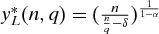 .
NON-MARKOV EQUILIBRIA
We have restricted our attention to symmetric Markov perfect equilibria. However, the legislative game we study is a dynamic game with an infinite horizon with many subgame perfect equilibria. The Markovian assumption of stationary strategies is very restrictive, and it is possible that some other equilibria can sustain more efficient outcomes through the use of history-dependent strategies (punishment and rewards for past actions).
This is common in infinite horizon games with perfect information. For instance, the only Markov perfect equilibrium of the infinitely repeated prisoner's dilemma has both players defect in every period. This is because in the prisoner's dilemma the state variable is null (i.e., all histories lead to strategically identical subgames), and the only Markov perfect equilibrium corresponds to the infinite repetition of the unique Nash equilibrium of the stage game. However, it is well known that cooperation can be sustained by history-dependent strategies with punishment (Aumann Reference Aumann, Luce and Tucker1959). Similarly, as we show next, in our legislative game the public good accumulation in the unique symmetric Markov perfect equilibrium is inefficient, but the optimal solution can be supported as the outcome of a subgame perfect equilibrium of the legislative game.
Proposition 4. For any q, there is a  such that for δ > the efficient investment path characterized by the optimal solution is a subgame perfect Nash equilibrium of the legislative game. Footnote 10
In the Appendix, we derive nonstationary strategies for the legislative game whose outcome is the efficient level of public good (the optimal solution) and show that these strategies are a subgame perfect Nash equilibrium. Footnote 11 We analyze separately the cases with q = 1, q = 2, . . ., n − 1, and q = n, because in the two extreme cases the potential for punishment is reduced.
In all cases, the strategy for the legislator recognized as the proposer is to propose the optimal level of investment, I*O(g), and to share equally among all committee members W − I*O(g) as private transfers. The voters’ strategy entails voting “yes” to a proposal in accordance with equilibrium if no prior deviation has been observed, and to switch to a punishment phase after a single deviation by any proposer. Deviation by voters (as well as deviations from punishment strategies) are punished in the same way as deviation by proposers.
For q = 2, . . ., n − 1, a deviation is punished by (a) rejecting an inefficient proposal, (b) stopping the accumulation of the public good, and (c) excluding the deviator from positive private transfers in any future proposal. For q = 1, the, proposer does not need the approval of any other member to implement a public policy, and therefore, there can be no punishment in the event he is recognized as the proposer. In this case, a deviation is punished by reversion to the Markov perfect equilibrium characterized in the previous section. For q = n, everyone's vote (including the deviator's) is needed to pass a punitive proposal, and thus, there is no enforceable harsher punishment than the status quo policy. In this case, a deviation is punished by implementing the status quo policy in all future periods.
The idea of the proof is simple: The required strategy configurations are such that any member who deviates from the prescribed proposal or from the prescribed punishment is certain to be punished. Members expect the punishment to be enforced because they expect that anyone who fails to punish a deviator will in turn be punished, and so on.
EXPERIMENTAL DESIGN
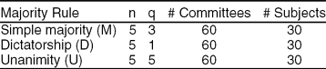
The experiments were all conducted at the Caltech Social Science Experimental Laboratory using students from the California Institute of Technology. Subjects were recruited from a database of volunteer subjects. Six sessions were run, using a total of 90 subjects. No subject participated in more than one session. In all sessions, the committees were composed of five members (n = 5), the discount factor was 3/4 (δ = 0.75), the exogenous amount of resources in each period was 20 (W = 20), and the current-round payoff from the public good was proportional to the square root of the stock at the end of that round ( , with α = 0.5).Footnote 12 Two sessions were run using a simple majority requirement to pass a proposal (q = 3, M), two sessions using a unanimity requirement (q = 5, U), and two sessions under a dictatorship rule (q = 1, D). Table 1 summarizes the theoretical properties of the equilibrium for the three treatments. It is useful to emphasize that, as proven in the previous section, given these parameters the steady state is uniquely defined for all treatments.
Experimental Parameters and Equilibrium

Discounted payoffs were induced by a random termination rule in which an eight-sided die was rolled after each round in front of the room, with the outcome determining whether the game continued to another round (with probability .75) or was terminated (with probability .25). This is a standard technique used in the experimental literature to preserve the incentives of infinite horizon games in the laboratory (Dal Bo Reference Dal Bo2005, Duffy and Ochs Reference Duffy and Ochs2009, Palfrey and Rosenthal Reference Palfrey and Rosenthal1994, Roth and Murnigham Reference Roth and Murnighan1978). All sessions were conducted with 15 subjects, divided into three committees of 5 members each. Committees stayed the same throughout the rounds of a given match, and subjects were randomly rematched into committees between matches. A match consisted of one multiround play of the game that continued until one of the die rolls eventually ended the match. As a result, different matches lasted for different lengths. Table 2 summarizes the design.
Experimental Design
Before the first match, instructions were read aloud, followed by a practice match and a comprehension quiz to verify that subjects understood the details of the environment including how to compute payoffs. The experiments were conducted via computers.Footnote 13 The current-round's payoffs from the public good stock (called project size in the experiment) were displayed graphically, with the stock of the public good on the horizontal axis and the payoff on the vertical axis. Subjects could click anywhere on the curve and the payoff for that level of public good that appeared on the screen.
In the M and U treatments, each round had two separate stages, the proposal stage and the voting stage. At the beginning of each match, each member of a committee was randomly assigned a committee member number, which stayed the same for all rounds of the match. In the proposal stage, each member of the committee submitted a provisional budget for how to divide the budget between the public good, called project investment, and private allocations to each member. After everyone had submitted a proposal, one was randomly selected and became the proposed budget. Members were also informed of the committee member number of the proposer, but not informed about the unselected provisional budgets. Each member then cast a vote either for the proposed budget or for the backup budget with zero public investment and equal private allocations. The proposed budget passed if and only if it received at least q votes. Payoffs for that round were added to each subject's earnings and a die was rolled to determine whether the match continued to the next round. If it did continue, then the end-of-round project size became the next round's beginning-of-round project size. The D treatment followed the same procedure for the proposal stage, but did not involve a voting stage: after everyone had submitted a proposal, one was randomly selected to be the committee decision in that round.
At the end of the last match each subject was paid privately in cash the sum of his or her earnings over all matches plus a showup fee of $10. Earnings ranged from approximately $20 to $50, with sessions lasting between one and two hours. There was considerable range in the earnings and length of sessions because of the random stopping rule.
EXPERIMENTAL RESULTS
Public Good Outcomes
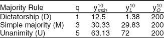
Median Public Good Stock. We start the analysis of the experimental results by looking at the long-run stock of public good by treatment. We consider as the long-run stock of public good the stock reached by a committee after 10 rounds of play.Footnote 14Table 3 compares the theoretical and observed levels of public good by treatment. To aggregate across committees, we use the median level of the public good from all committees in a given treatment at round 10 (y10mdn). Similar results hold if we use the mean or other measures of central tendency.Footnote 15 We compare this to the stock predicted by the Markov perfect equilibrium of the legislative game after 10 periods (y 10L) and to the stock accumulated in the optimal solution after 10 periods (y 10O).
Long-Run Stock of Public Good, Theory vs. Results by Treatment
How do committees get to these stocks of public good? Figure 3 gives us a richer picture, showing the time series of the stock of public good by treatment.Footnote 16 The horizontal axis is the time period, and the vertical axis is the stock of the public good. As in Table 3, we use the median level of the public good from all committees in a given treatment. Superimposed on the graphs are the theoretical time paths (represented with solid lines), corresponding to the Markov perfect equilibria and to the optimal solution.
Median Time Paths of the Stock of g, All Treatments

Table 3 and Figure 3 exhibit several systematic regularities, which we now discuss in comparison with the theoretical time paths.
FINDING 1. Higher q leads to higher public good production:Dictatorship leads to lower public good production than simple majority and unanimity; unanimity leads to higher public good production than simple majority. According to t-tests,Footnote 17 the average stock of public good is significantly lower in D than in U in every single period. This difference is statistically significant at the 1% level (p-value < 0.01) in every period. The stock of public good is larger in M than in D and larger in U than in M in every single period. These differences are statistically significant for periods 1 through 6. Footnote 18 The lack of statistical significance for the later rounds is due to the small sample size for the M treatment.Footnote 19
Not only are the differences statistically significant but they are also large in magnitude. The median stock of public good is two times greater in the U treatment than in the D treatment, averaged across all 13 rounds for which we have data (20.1 in D vs. 31.7 in M vs. 39.8 in U). The differences between the three voting rules are relatively small in the initial round, but they increase sharply as more rounds are played. By round 10, the differences are very large (12.5 vs. 30.3 vs. 63.1).
FINDING 2. All voting rules lead to significantly inefficient long-run public good levels. The optimal steady state is y*=400, and the optimal investment policy is the fastest approach: Invest W in every period until y* is achieved. After 10 rounds, the median stock of public good achieved with the optimal investment trajectory is 200. With a legislature, the median stock of public good levels out at about 15 under dictatorship, at about 30 under simple majority, and at about 60 under unanimity. The median stock averages 14.5 in rounds 7–10 in D, 31.8 in rounds 7–10 in M, and 57.9 in rounds 7–10 in U. These very inefficient long-run public good levels occur in spite of initial round median investment that is fully efficient (I=W) in M and UFootnote 20 and very close to efficiency (I=0.94W) in D. In all treatments the average stock of public good in the last rounds (rounds 8 on) is significantly smaller than the level predicted by the optimal solution (the level attainable investing W each round) according to the results of a t-test on the equality of means (p-value <0.01).
FINDING 3. In all voting rules, there is overinvestment relative to the equilibrium in the early rounds. This is followed by either negative investment (in the D and the M treatment) or by zero investment (in the U treatment) approaching the theoretical predictions. The median investment levels in the first two rounds are (18.8, 11.3) in D, (20, 18.3) in M, and (20, 20) in U. As a result the median public good stock by the end of round 2 equals, respectively, 26.3, 26.83, and 40. This compares with equilibrium investment policies in the first two rounds equal to (1.38, 0) for D, (8, 6) for M, and (6, 6) for U, and a predicted stock equal to 1.38 for D, 14 for M, and 12 for U.Footnote 21 Thus, in all treatments, committees overshoot the equilibrium in early rounds by a factor of 20 (D), 2 (M), and 3 (U). This overshooting is largely corrected in later rounds, either via disinvestment (in D and M) or an arrest in investment (in U). In the M treatment, convergence is especially close to equilibrium, with the difference between the median public good levels and the equilibrium public good levels in the last four rounds of data measuring less than 2 units of the public good (31.79 vs. 29.83). A similar pattern of overshooting in the D mechanisms is also evident. Beginning in round 4, the stock of public good in D declines sharply, with the median public good stock averaging 16.6 in rounds 4–10. In U, the investment slows down considerably after the second round: The median investment in rounds 3–10 is 0. Given the nature of the equilibrium investment function for this voting rule (a convex function), the investment cessation following the initial overshooting brings the level of the stock closer to the predicted one and eventually, below it (the median stock in round 10 is 63.1 vs. a predicted stock of 72).
The pattern of early overinvestment in the public good (relative to equilibrium), followed by later convergence to equilibrium investment levels, echoes findings of many static public goods experiments with voluntary contributions, which are typically repeated for 10 or more repetitions with the same group. A typical pattern in those experiments is that groups tend to briefly attain public good levels significantly higher than the Nash equilibrium in early periods, which then declines in later periods, converging toward the equilibrium public good levels. We see something similar in our data. This pattern may appear to be “cyclical” in the sense of the public good stock overshooting the equilibrium steady state and then converging back down toward the steady state. However, the pattern of investment over time is monotonically declining investment in the public good. Also, note that from the standpoint of the theoretical equilibrium, there is not “underinvestment” in later periods. Rather, there tends to be overinvestment (relative to the theoretical benchmark) in early periods and behavior closer to equilibrium in later periods.
Variation across Committees
Because of the possibility of nonstationary equilibria it is natural to expect a fair amount of variation across committees. Figure 3, by showing the median time path of the stock of public good, masks some of this heterogeneity. Do some committees reach full efficiency? Are some committees at or below the equilibrium? We turn next to these questions.
Figure 4 illustrates the variation across committees by representing, for each round, the first, second, and third quartile of investment levels for the D (panel (a)), M (panel (b)), and U game (panel (c)).
Quartiles of Time Paths of g, (a) dictatorship, (b) simple majority, and (c) unanimity

There was remarkable consistency across committees, especially considering this was a complicated infinitely repeated game with many non-Markov equilibria.Footnote 22 A few committees invested significantly more heavily than predicted by the Markov perfect equilibrium, but this only happened rarely, and nearly always such cooperation fell apart in later rounds. The most efficient committee in M invested W in each of the first 7 rounds, resulting in a public good level of 140. That committee did not invest anything for the remaining two rounds. Even this very successful committee stopped investing well short of the efficient level. The most efficient committee in D invested W in each of the first four rounds, resulting in a public good level of 80. That committee disinvested the entire stock of public good in the following round. In U only two committees reached levels above 80, and not a single committee invested W for more than four consecutive rounds.
These findings are perhaps surprising because, from Proposition 4, we know that, for the parameters of the experiment, the optimal solution can indeed be supported as the outcome of the game in M and U using nonstationary strategies (at least for the first 10 rounds).Footnote 23 In D, even if the parameters of the experiment do not allow an efficient level of the public good to be attainable in equilibrium, using nonstationary strategies can sustain a level of the public good much higher than the one predicted by the Markov perfect equilibrium, namely around 50 (with respect to 1.38). Figure 3 and 4, therefore, make clear that the predictions of the Markov perfect equilibrium are substantially more accurate in all three voting rules than the prediction of the “best” subgame perfect equilibrium (that is the Pareto superior equilibrium from the point of view of the agents), even when this best equilibrium is unique and reasonably focal (being the efficient solution). This observation may undermine the rationale for using the “best equilibrium” as a solution concept.
Proposals and Coalitions
We now turn to a descriptive analysis of the proposed private transfers of the current consumption good, as a function of g and q. For this analysis we focus primarily on the number of members receiving significant positive tranfers in the proposed allocation and whether the proposals had negative investment in the public good. We break down the proposed allocations into four canonical types: (1) Invest W: 100% allocation to the public investment; (2) Proposer only: the allocation divided between public investment and private consumption of the proposer only; (3) Proposer + 2: the allocation divided between public investment and a coalition that includes the proposer and two other members of the committee (notice that this is a minimal winning coalition in M); and (4) Universal: positive private allocations to all five members.Footnote 24 The last three categories are further broken down by whether investment in the public good is positive, zero, or negative.
Table 4 shows the breakdown of proposals for the three treatments. In each treatment, the first column lists the proportion of proposals of each type that were proposed at the provisional stage (i.e., before a proposal was randomly selected to be voted on). The second column gives the proportion of proposals of each type that passed when they were voted on.
Proposal Types

Note: Number of observations: 1,650 for D, 1,084 for M, and 1,290 for U.
FINDING 4. In all treatments, most proposals are either (i) invest the entire budget or (ii) universal private allocations with positive investment. The proportion of proposals that belong to these two categories increases with the majority requirement adopted. With all voting rules, most proposals were to either invest W or universal allocations with a positive amount of investment. In D, these two proposal types account for 46% of all budget proposals (including provisional budget proposals); in M and U, these two types account, respectively, for 60% and 86%. Proposals that offered private allocation to the proposer only were quite rare in M and U, but not in D (where they account for 37% of all provisional proposals). Proposals with zero or negative investment occurred 26% of the time in D committees, 23% of the time in M committees, and 10% of the time in U committees. In contrast to the data, the Markov perfect equilibrium proposals should have been concentrated in the two categories: “proposer only” and MWC. However, it should be noted that even when transfers are provided to more than a minimum winning coalition, it is concentrated on a minimum winning coalition.
Because one of the most common proposal types is one that offers some positive transfer to all members of the committee, it is interesting to check whether transfers are egalitarian or whether they are mainly concentrated on a minimal winning coalition of voters. Figure 5 shows the cumulative distribution of transfers in provisional proposals when committee members are indexed in decreasing order of their allocation.
Cumulative Distribution of Private Transfers, All Treatments

FINDING 5. In D and M, a minimal winning coalition of players receives a more than proportional share of transfers. In U, transfers tend to be more egalitarian. In the D treatment, 75% of the private transfers go to the proposer. In the M treatment, 80% go to the proposer and two other minimum winning coalition partners, and more than 90% go to the proposer and three other committee members. Thus, universal allocations are not even close to equitable in the sense of giving all coalition members the same allocation. In U, proposed allocations of the private good are relatively equitable; the proposer is allocated 23%, and the member allocated the least receives 19% on average. The observations about proposed transfers, summarized in Findings 4 and 5, are similar to findings in other experiments on legislative bargaining (Frechette, Kagel, and Lehrer 2003; Frechette, Kagel, and Morelli 2012) and take-it-or-leave-it bargaining. For example, even in the simplest bargaining game—the ultimatum game— proposers offer somewhat more than the equilibrium offer to be sure the responder will “vote” for it (Guth Schmittberger, and Schwarze Reference Guth, Schmittberger and Schwarze1982).
Voting Behavior
Testing for Non-myopic Behavior.Table 5 displays the results from logit regressionsFootnote 25 where the dependent variable is vote (0 = no; 1 = yes). An observation is a single voter's vote decision on a single proposal.Footnote 26 The proposer's vote is excluded.Footnote 27 The data are broken down according to the treatment (M or U). The independent variables are EU(status quo), the expected value to the voter of a “no” outcome (including the discounted theoretical continuation value), and EU(proposal), the expected value to the voter of a “yes” outcome. Theoretically, a voter should vote yes if and only if the expected utility of the proposal passing is greater than or equal to the expected utility of the status quo. This would imply a negative coefficient on EU(status quo) and a positive coefficient on EU(proposal), with the magnitudes of these coefficients being approximately equal.
Logit Estimates

Notes: Dependent var: Pr {vote=yes}. SE clustered by subject in parentheses; * significant at 10% level; ** significant at 5 significant at 5% level; *** significant at 1% level.
FINDING 6. Voter decision making is non-myopic. The results from Tables 5 are clear. The main effect on voting is through the difference between the expected utility of the status quo and the proposal. The signs of the coefficients are highly significant, large in magnitude, and not significantly different from each other in absolute value. The constant term is not significantly different from zero or weakly significant (only in one specification), suggesting that voters are not a priori inclined to favor or disfavor proposals.
Proposal Acceptance Rates. The theory predicts that all proposals should pass. Is this consistent with the data? Table 4 displays the probability that the proposal will pass for M and U proposals.
FINDING 7. The vast majority of proposals pass.Overall, 82% of the M proposals and 69% of the U proposals receive committee support. Many of the M proposals are unanimously supported, especially the “invest W” proposals and the universal proposals with positive investment.Footnote 28
Acceptance rates differ by type of proposal. Some kinds of proposals are rejected somewhat frequently. This is particularly true for proposals with negative investment. In M committees, only 57% of proposals with negative investment pass, and in U committees, only 19% pass. Proposals that give private allocation only to the proposer also fare relatively poorly, passing 81% of the time in M committees and 0% of the time in U committees. The most common proposal types, “invest W” and universal with positive investment, nearly always pass. The acceptance rates for proposals to invest everything are 98% and 80% for the M and U treatments, respectively. The corresponding acceptance rates for universal proposals with positive investment are 93% and 68%. One surprise in the data is the relatively low acceptance rates for MWC proposals in M.
Even if our legislative game is different from the standard Baron-Ferejohn setting, it is interesting to note that these numbers are in line with the acceptance rates for first-round proposals in experiments testing that bargaining protocol (with simple majority): In Frechette, Kagel, and Morelli (2003) 96.4% of first-round proposals are accepted (closed rule treatment), whereas in Kagel, Sung, and Winter (2010) 89% of first-round proposals pass when the cost of delay is high and 72% pass when the cost of delay is low (both numbers refer to the control treatment without a veto player).
Table 6 instead displays the percentage of accepted proposals that are predicted by the theory to be accepted and the percentage of refused proposals predicted by the theory to be refused, divided by proposal type. Theoretically, legislators should support a proposal if the expected value to them of a “no” outcome (including the discounted theoretical continuation value) is smaller than the expected value to them of a “yes” outcome. We say that theory predicts a proposal to pass in M (U) if the expected utility of the proposal passing is greater than or equal to the expected utility of the status quo for at least three (for all five) legislators.
Proposal Acceptance Rates, Theory versus Experiments

Notes: “% Acc as Pr” is the percentage of accepted proposals that theory predicts to pass and “% Ref as Pr” is the percentage of refused proposals that theory predicts to be refused. The number of observations is in parentheses.
The theory does remarkably well. Overall, the voting outcome is correctly predicted by the theory around 85% of the times for M and around 70% of the time for U. The cases that the theory fails to predict are proposals with positive investment that should be rejected but instead pass and proposals with negative or no investment that should be accepted but instead fail.
One possible explanation for this discrepancy between voting behavior and theoretical prediction is that, rather than playing a stationary equilibrium, some committees are supporting more efficient allocations by using nonstationary strategies. This possibility is in line with recent experimental results on repeated games: Dal Bo (Reference Dal Bo2005) and Dal Bo and Frechette (Reference Dal Bo and Frechette2011) suggest the likelihood that in these games the infinite horizon dynamics allow efficient or nearly efficient public goods provision.
Behavioral Factors Affecting Voting. We next explore the extent to which voting behavior depends on factors other than just the expected utility from the status quo and the expected utility from the current policy proposal (this is the basic assumption from the Markov perfect equilibrium). For instance, the voting behavior could be affected by nonstationary strategies or other-regarding preferences. Table 7 reports the results of a logit regression of voting behavior on the same variables in Table 5, but includes four additional regressors that could indicate some degree of punishment or reward behavior being used to affect proposals and support equilibrium outcomes that differ from the theoretical stationary solutions: the proposed investment level I; a Herfindahl index, h, that captures how unequal the proposed allocation of private good is across committee members; P, the amount of private allocation offered to the voter; and the amount of own-private allocation by the proposer (that we call “greed”). In the case of nonstationary behavior, the sign on I should be positive (in the sense that voting strategies punish proposals that do not offer sufficient public good), whereas the sign on h and greed should be negative (in the sense that greedier or less egalitarian proposals are punished with more negative votes).
Logit Estimates

Notes: Dependent var: Pr {vote=yes}. SE clustered by subject in parentheses; * significant at 10% level; ** significant at 5% level; *** significant at 1% level.
The results are presented in Table 7. First, we notice that adding these new variables does not change the main result from Table 5: The coefficients on EU(status quo) and EU(proposal) still have the correct (opposite) signs, are not significantly different from each other, and are highly significant. Some of the new factors we introduced in our analysis in Table 7 are statistically significant, but have a smaller impact. For the M treatment, all three of the “nonstationary” variables have the expected sign, and two are highly significant (I and greed). More efficient proposals receive greater support, as do proposals that are less greedy. The size of the positive sign of the effect of I, however, seems too small to provide evidence in favor of an equilibrium in which non Markovian strategies reward efficient behavior, especially because a positive sign is consistent with equilibrium behavior.Footnote 29 Therefore we are reluctant to conclude that the significant coefficient on I is indicative of nonstationary behavior. In contrast, the significance of the coefficient of greed demonstrates the existence of voting behavior that rewards exactly the types of proposals we see more of relative to the equilibrium predictions (invest W and universal). Results for the U treatment are similar, but the new variables have less importance in explaining the variance in voting behavior: I, h, and greed all have the right sign, but here only I is (weakly) significant.
Behavioral Factors Affecting Proposals. Finally, we look at how current proposals treat the proposer of the previous round, depending on how a current proposer was treated by the last proposer. The hypothesis is that how well the current proposer treats the previous proposer increases according to how well the previous proposer treated him of her. Because the only way the current-round's proposer can target a punishment or reward for the previous round's proposer is with private transfers, we run a regression where the dependent variable is the current proposal's private allocation to the previous round's proposer. For observations, we use all current-round provisional budgets beginning in round 2, excluding the provisional budget of the previous round's proposer. In Table 8, we report one regression for each treatment. The independent variables we use for how well the previous round's proposer treated the current-round proposer are lagged versions of EU(proposal), and of the I, h, and greed variables. In other words, we check whether there are lagged effects of efficiency or fairness of the previous proposal on the current proposal's private allocation to the previous proposer.
TOBIT Estimate

Notes: Dependent var: Private allocation offered to previous round's proposer. SE clustered by subjects in parentheses; * significant at 10% level; ** significant at 5% level; *** significant at 1% level.
The coefficient on EU(proposal)t − 1 is always significant. There is a significant effect of the lagged greed variable in M and in D and a significant effect of lagged investment in M and U.
We conclude from this analysis that there is some evidence of the use of nonstationary strategies, but that subjects are non-myopic: The main determinant of voting is the difference between the expected utility of the status quo and the proposal, taking into account anticipated future payoffs. In proposal behavior, current proposals discriminate against previous proposers who were too greedy (in M and D) or invested in the public good (in M and U). The nonstationarity in behavior seems to be motivated by spite rather than by efficiency considerations.
DISCUSSION AND CONCLUSIONS
This article investigated the dynamic provision of durable public goods by a legislature, operating with procedures that entail bargaining and voting. Despite the fact that most, if not all, public goods provided by governments are durable, very little is known on this subject, both from a theoretical and empirical point of view. We attempt to provide a first answer to some basic questions that can be a helpful starting point for further research on the politics of dynamic public good provision.
We ask two main questions: Do legislatures provide public goods efficiently in a dynamic setting? To what extent does this efficiency depend on the voting rule adopted by the floor? The theoretical properties of the Markov perfect equilibrium in our legislative bargaining game imply that the steady-state level of public investment approved by a legislature is inefficiently low for any voting rule but unanimity: The inefficiency of the long-run steady state decreases with the majority requirement adopted and disappears completely when a proposal on resources allocation passes only with a unanimous vote. However, even with unanimity, convergence to the steady state is inefficiently slow, because the proposer will appropriate rents along the path.
Our model, with supporting evidence from a laboratory experiment, identifies an important force by which supermajority voting systems may increase efficiency in the provision of durable public goods. Of course, there are some forces outside the model that may work in the opposite direction. Buchanan and Tullock (Reference Buchanan and Tullock1962) argue that supermajority requirements can increase transaction or bargaining costs in the decision-making process (but reduce external costs, as in our model). Unanimity and near-unanimity rules can create political hold-up problems; Barry (Reference Barry1965) argues this point in the context of legislative bargaining and pork-barrel politics. Although such arguments have generally been made mainly in the context of static models, part of the benefits of higher q that we find arise out of the dynamic nature of the public decision in our model, which is different from earlier models. The extent to which those various intuitions about the various effects of q on transaction and external costs apply more broadly in dynamic political decision making is an important open question. Our work contributes to this literature by highlighting an additional cost associated with bargaining in legislatures with unanimity that was not previously considered: Unanimity may lead to an efficient steady state, but the speed of convergence is inefficiently slow. The delay in investment may generate a significant loss of welfare.
The experimental analysis of three alternative voting rules (simple majority and the two polar extremes, dictatorship and unanimity) supports these key predictions. A higher majority requirement leads unambiguously to significantly higher public good production. This result confirms, from an experimental point of view, the importance of institutions in public good provision and the fact that incentives matter in a way predicted by complex theoretical models. In all cases, investment is generally below the Pareto efficient levels, regardless of the voting rule used. Although we often observe more investment than predicted in the early stage of the game, overinvestment does not persist: The long-run public good levels approximate the Markov perfect equilibrium steady state.
The final questions we attempt to address are as follows: To what extent are the models we use adequate to study this problem? What equilibrium concepts should be used? This latter question is a particularly important one because, depending on the equilibrium concept, we can have very different predictions for the same model. It is clearly difficult to identify the equilibrium adopted by players, but the analysis of proposal and voting behavior provides some interesting insights. First, as discussed in the section, “variation across committees,” we observe a consistent pattern of behavior across committees, despite the fact that we have a multiplicity of potential equilibria. The Markov perfect equilibrium that we have adopted as a benchmark does not fully capture the complexity of the agents’ strategies, which also depends to a limited extent on other factors, as shown in Table 7. However, these nonstationary effects are small, and the Markovian equilibrium benchmark is far closer to the data than the prediction of the best subgame equilibrium sustainable with nonstationary strategies, the alternative benchmark that is routinely applied when studying cooperation in repeated games. In our setting, this alternative would predict efficient outcomes for any q>1, which is far off the mark.
There are many possible directions for the next steps in this research. On the experimental side, our design was intentionally very simple and used a limited set of treatments. The theory has interesting comparative static predictions about the effect of other parameters of the model that we have not explored in this work, such as the discount factor, the production technology, preferences, and endowments. The theoretical model is easily adapted to these extensions. For example, a higher discount factor increases both the optimal steady state and the equilibrium steady state of the durable public good for all values of q and n. For similar reasons positive depreciation in the public good technology leads to a decrease in the steady state of the Markov equilibrium studied here.
We have also limited the analysis to legislatures that differ on the q-rule adopted and use a specific procedure. It would be interesting to consider the impact of different proposal and voting procedures (e.g., alternating offer bargaining without a status quo alternative, à la Baron and Ferejohn Reference Baron and Ferejohn1989). Moreover, our political process does not have elections and parties, and there is no executive branch or “president” to oversee the general interest common to all districts. Elections, parties, and nonlegislative branches are all important components of democratic political systems, and incorporating such institutions into our framework would be a useful and challenging direction to pursue. Finally, it would be interesting to allow for a richer set of preferences and feasible allocations, such as allowing for diversity of preferences or multiple public goods.
APPENDIX: PROOFS OF PROPOSITIONS OPTIMAL PUBLIC POLICY
In the steady state y(y*O) = y*O and x(y*O) > 0. Because y(g) is constant for g ≥ max {y*O − W, 0}, it is straightforward to show that the derivative of the value function in this region is  . Using the first-order condition for optimality, we must have nu′(y*O) + δ = 1, so

Proof of Proposition 1
Define a function

where  . Note that this function is continuous, increasing, concave, and differentiable with respect to g, with
 . Now define (g) implicitly by the equation:

This equation can be rewritten as

Note that (11) implicitly defines a differentiable and increasing function of g. To see this, note that differentiating (11) with respect to and g gives

We can therefore define a point gL 2 = min[g ≥ 0 | (g) ≥ yL*. This point has the property that for any g ≥ g 2L, we have (g) ≥ yL*; moreover, g 2L < y*L. Now define the function

Let g > 0 be defined by g = u′ −1(1). We have Lemma A.1.
Lemma A.1. There is a such that for δ > , (g) and v 2L(g) are increasing and continuous and concave, respectively in g ∈ [g, gL 2, and in g ≥ g 2L.
Proof. We showed earlier that ′(g) > 0. Furthermore, differentiating (12) with respect to g, we have

It is clear that there is a such that for δ > , ″(g) < 0 for any g ∈ [g, gL 2]. To see this, note that for δ = 1 we have ″(g) ≤ 0, because the numerator of (14) is smaller than 0 and its denominator is greater than 0, and recall that (g) is continuous. For v 2L(g), note that for g ≥ g 2L the function is linear. For g ≤ g 2L

so concavity in g, gL 2 follows from the concavity of (g) for δ sufficiently large. Concavity in g ≥ g 2L follows from the fact that in this range v 2L(g) is differentiable everywhere except at most at g 2L, and its derivative is non increasing in g. ■
Define y 1* = arg maxy′ {u(y′) − y′ + δvL 2(y′)} and gL 1 = min [g ≥ 0 | (g) ≥ y 1*]. Note that  , an upper bound that is independent of W, and g 1L ≤ g 2L; moreover, g ≤ g 1L, implies (g) ≤ y 1*. We can now construct the following value function:

which is a continuous and nondecreasing function of g. We can also construct the strategies
![\begin{equation*}
y_{L}^{\ast }(g) = \left\lbrace \begin{array}{c@{}c}y_{1}^{\ast } & g\le g_{L}^{1} \\
[5pt] \widetilde{y}(g) & g\in \left( g_{L}^{1},g_{L}^{2}\right] \\
[5pt] y_{L}^{\ast } & else \end{array} \right.
\end{equation*}](https://static.cambridge.org/binary/version/id/urn:cambridge.org:id:binary:20160312035210217-0934:S0003055412000160_eqnU9.gif?pub-status=live)
and x*L(g) = W − yL(g) + g − (q − 1)sL(g). We now show that the value function v*L(g) and the strategies y*L(g) and x*L(g) are an equilibrium for a sufficiently large W and δ. Consider the proposer's problem (5). One of two cases is possible. First, the incentive compatibility (IC) constraint is not binding, so the proposer can effectively ignore the other legislators. Second, the IC constraint binds and so the proposer has either to increase the level of public good, provide positive transfers to a minimal winning coalition, or both.
Case 1: Nonbinding IC. Assume first that we can ignore the IC constraint and set s = 0. The problem becomes:

If we ignore the constraint in (15), then it is optimal (without loss of generality) to choose y such that

It is useful to have the following result:
Lemma A.2. The threshold g 1Lis a nonincreasing continuous function of W, and for any ϵ there is a W ϵsuch that for W > W ϵ, then g 1L ≤ ϵ.
Proof. Let k be defined as before by u′(k) = 1. Then because v 2L(y) is nondecreasing in y, y*1 ≥ k > 0. Let f(W) be defined by

So g 1L = max {0, f(W)}. Because f(W) is a continuous decreasing function of W, it is then immediate that g 1L is a continuous and monotonically nonincreasing function of W. It is also immediate to verify that for any ϵ>0 there is a W ϵ such that g 1L ≤ ϵ for W > W ϵ. ■
By Lemma A.2 we can find a W 1 such that for W > W 1, g 1L is sufficiently small to guarantee that u′(y) + δv*′L(y)>1 for any g ≤ g 1L, so

implies y > g 1L. Lemma A.1 then guarantees that for δ ≥ the unique solution to (15) is y*1. It is easy to see that in correspondence to y*1 we have xL(g) ≥ 0 if and only if g is greater than or equal to max {y*1 − W, 0}. Because y*1 is bounded, this is verified for any g ≥ 0 when W > W 1, and W 1 is chosen to be sufficiently large. The IC constraint is satisfied if and only if (g) ≤ y 1*; that is, if g ≤ g 1L. We can therefore conclude that, for δ > and W > W 1, when g ≤ g 1L the optimal policy is y*L(g) and x*L(g).
Case 2: Binding IC Constraint. When g > g 1L the IC constraint cannot be ignored. In this case, the problem solved by the proposer is

Note that we can assume without loss of generality that the solution to this problem is larger or equal than y*1 (if this were not the case, by increasing y the proposer would increase his utility and relax the constraint, a contradiction). By Lemma A.1, it follows that we can treat (17) as a concave maximization problem when δ ≥ . There are two possibilities. First, the proposer continues to provide no consumption to the districts of other legislators, but he increases the provision of the public good yL(g) to satisfy the incentive compatibility constraint (no transfer case). Second, he provides consumption to the districts of q − 1 other legislators and to his own district (transfers case).
Consider the second case first, assuming s > 0. We can write (17) as

where Ψ(·) = u(·) + δvL(·). Choosing an optimum in problem (18) is equivalent to choosing an optimum in problem: max y{qΨ(y) − y}. So an optimal choice for the proposer is to propose yL(g) = y*L This case is feasible only if  , that is if and only if g ≥ g 2L. In the case in which g ∈ [g 1, g 2] then we must have
 , so the chosen y is (g). It follows that in this range the optimal proposal is y*L(g) and x*L(g).
Finally, we need to show that v*L(g) is the expected utility of a player when the strategies are y*L(g), x*L(g). This is immediate for g > g 2L. For g ∈ [0, g 2L], observe that, by a similar argument as in Lemma A.2, for any γ there is a W γ such that for W > W γ, then (y 1*) > γ. It follow that when W > W gL 2, yL*(g) = (g)>gL 2 for any g ∈ (g 1L, g 2L], so in this range the value function is given by (13). Finally it is easy to see that for W > W gL 2, ((g)) ≥ (y 1*) > gL 2, so the value function is v*L(g) in [0, g 2L]. We conclude that there is a , such that for δ > and W > the value function v*L(g) and the strategies y*L(g) and x*L(g) are an equilibrium.
Proof of Proposition 2
Fix q, W, δ, and n, such that δ > and W > as defined in Proposition 1. Consider any regular equilibrium v(g), y(g), x(g), with steady state y*. We need to prove that  . The IC constraint in state g if policy y(g) is chosen is

where Ψ(·) = u(·) + δv(·). In the steady state, this condition becomes:  . In equilibrium, this constraint is satisfied with equality (if not, the proposer could decrease s and be better off). The proposer's policy must therefore solve

By continuity of Ψ(·), for any g in a neighborhood of y*, s(g) > 0. By continuity of the value function, this implies  in a neighborhood of y*, implying
 . This fact, together with the first-order necessary condition of (19) (qu′(y)+qδv′L(y) = 1), implies
 . ■
Proof of Proposition 3
We first prove the claims regarding the steady state. The unique equilibrium steady state in the optimal solution is  and the unique equilibrium steady state in the legislative game is
 . Notice that
 for any q = 1, . . .n, n > 0, and δ > 0. Because u(·) is, by assumption, increasing and concave (i.e., u′(g) > 0, u′′(g) ≤ 0), this implies that y*O ≥ y*L for any q = 1, . . .n, n > 0, and δ > 0. This inequality is strict when q = 1, . . .n − 1 (i.e., when n/q > 1) and y*O = y*L when q = n (i.e., when n/q = 1). Moreover, notice that
 is monotonically decreasing in q. Therefore, y*L is monotonically increasing in q. Because y*O is independent of q, this also means that the efficiency of the equilibrium steady state in the legislative game is monotonically increasing in q.
We now want to show that—with n > 1 and q = n—even if y*L = y*O, the convergence to y*L is slower than the convergence to y*O. To do this, we compare the two investment functions, IO(g) and IL(g):
![\begin{eqnarray*}
I_{O}(g) &=&\min \left\lbrace W,y_{O}^{\ast }-g\right\rbrace \!. \\
I_{L}(g) &=&\left\lbrace \begin{array}{c@{}c}y_{1}^{\ast }-g & g\le g_{1} \\
[5pt] \widetilde{y}(g)-g & g\in \left( g_{1},g_{2}\right] \\
[5pt] y_{L}^{\ast }-g & else. \end{array} \right.
\end{eqnarray*}](https://static.cambridge.org/binary/version/id/urn:cambridge.org:id:binary:20160312035210217-0934:S0003055412000160_eqnU13.gif?pub-status=live)
First notice that, when n > 1, y*L = y*O > y*1 and y*L = y*O > (g) for any g ≤ g 2. There are two cases: (1) g 1 = 0 and (2) g 1 > 0. If g 1 = 0, for any g ≤ g 2, IL(g) = (g) −g, which is smaller than IO(g) = min {W, y*O − g}. If g 1 > 0, for any g ≤ g 1, IL(g) = y*1 − g ≤ W for any g ≤ g 1 and IL(g) = y*1 − g ≤ y*O − g for any g ≤ g 1 (because y*O > y*1). This implies IL(g) ≤ IO(g) = min {W, y*O − g} for any g ≤ g 1. ■
Proof of Proposition 4
A) q = 2, . . .n − 1. To support the optimal stock of the public good as the outcome of a subgame perfect Nash equilibrium, employ the following strategy configuration:
1. Whenever a member is recognized, he proposes a public policy x, which entails a level of investment equal to I*O(g) and an even share of W − I*O(g) as private transfer to all committee members; everyone votes in favor of x (i.e., the proposal is implemented).
2. If a member j is recognized and deviates by proposing y ≠ x, every i ≠ j votes against the proposal; from the following period on, whenever j is the proposer, every i ≠ j votes against any proposal, and whenever i ≠ j is the proposer, I propose to divide W equally among all members but j as private transfers; every i ≠ j votes for this proposal (i.e., a punishment is carried on in all future periods in which the deviator is the proposer; when the deviator is the proposer, the status quo is implemented).
3. If a member k deviates by voting contrary to the strategies above or if member k deviates from the prescribed proposal in the punishment phase, implement the punishment in strategy 2 with k replacing j.
We first show that the proposer has no profitable deviation from the equilibrium strategy on the equilibrium path. The proposer's payoff if she follows the equilibrium strategy is

where

According to the proposed equilibrium voting strategies, whenever the proposal is different from the equilibrium one, a punishment will be carried out in every future period in which the proposer is not the deviator and the status quo will be implemented in all the other periods. Thus, all deviations are payoff equivalent. The proposer's payoff if she deviates is:

where

To check that the proposer's strategy is an equilibrium it is sufficient to check that the proposer has no profitable deviation. Notice that the expected payoff from a deviation is lower than the payoff that would derive from implementing the status quo for the current and all future periods. We can, thus, check that the expected payoff from the equilibrium strategy is higher than the payoff from implementing the status quo forever. We have three cases, depending on the region of the state space we are in:
Case 1:g ∈ [gO, y*O). In this case, we want to show that:

This inequality holds for any δ ∈ [0, 1]. To see this, note that by concavity of u(·)and the optimality condition in the efficient solution we have  for any x ≤ y*O.
Case 2:g ∈ [0, gO) & (g + W) > gO. In this case, we want to show that

where

Therefore the inequality we want to check becomes

Using the fact that  we have a lower bound on the LHS and we can plug it in to have

This inequality holds for δ ≥ ∈ [0, 1].
We can find a lower bound on δ using the actual VDEV(g) rather than the expression we used above (given by the expected utility of implementing the status quo for any period following a deviation that is greater than VDEV(g) for any g). In this case, the inequality we want to prove is

Using the fact that  we have a lower bound on the LHS and we can plug it in to have

This inequality holds for δ ≥ ∈ [0, 1]. To see this, note that the LHS is always positive, whereas the RHS is nonpositive as long as  —(because n > 1 and W > 0 and in this region g∈(y*O − 2W, y*O − W).
Case 3: g ∈ [0, gO) & (g + W) ≤ gO. Here we want to prove the following inequality:

where VEQ(g + W) = u(g+2W) + δVEQ(g+2W).
Note that, because  for any x ≤ y*O, we have
 if (g + x) ≤ y*O. Using this inequality we have a lower bound on the RHS, and it is sufficient to prove that

Note that V′EQ(x)>1/n for any x ≤ y*O (as it is clear from the equation for VEQ(y*O) and the condition for optimality in the efficient solution), and thus,  . This gives us a lower bound on VEQ(g+2W)
 that we can use to get a lower bound onVEQ(g + W):

It is therefore sufficient to show that

This inequality holds for any δ ∈ (0, 1).
Next, we need to prove that there is no profitable deviation from the prescribed voting strategy on the equilibrium path (i.e., that the expected utility from voting “yes” to an equilibrium proposal is weakly higher than the expected utility from voting “no”). A unilateral deviation in the voting stage does not change the outcome (i.e., the efficient proposal will be implemented), and the only difference in the two expected utilities (voting “yes” vs. voting “no”) is in the continuation values, VEQ(g) and VDEV(g), which are the same as the ones specified for the proposer (because the punishment takes the same form). We have three cases:
Case 1: g ∈ [gO, y*O). The inequality we need to show is

which clearly holds for any δ.
Case 2: g ∈ [0, gO) & (g + W) > gO The inequality we need to show is

Notice that  . This gives us a lower bound on the LHS, y*O/n − g/n − W/n. Therefore we can check the following inequality:

Case 3: g ∈ [0, gO) & (g + W) ≤ gO The inequality we need to show is:

As noted earlier,  . This means that we can prove the following inequality instead:

For δ ≥ 1/n, the RHS is negative, whereas the LHS is always positive, which gives the desired result.
Next, we need to prove that there is no profitable deviation from the prescribed voting strategy in the punishment phase (i.e., that the expected utility from voting “yes” to the punishment proposal is weakly higher than the expected utility from voting “no”):

It is clear that this inequality holds for any δ ∈ [0, 1].
Finally, we need to prove that there is no profitable deviation from the prescribed proposal strategy in the punishment phase. Any deviation will lead to rejection of the proposal and, thus, implementation of the status quo. This means that a proposer different from the deviator will stick to the punishment proposal as long as

which clearly holds for any δ ∈ [0, 1] and were done. ■
B) q = n. In this case, following a deviation, the status quo will be implemented every period. This is because—in the punishment phase—the deviator never accepts a proposal with an harsher punishment and his vote is needed to pass any proposal. To support the optimal stock of the public good as the outcome of a subgame perfect Nash equilibrium, employ the following strategy configuration:
1. Whenever a member is recognized, he proposes a public policy x, that entails a level of investment equal to I*O(g) and an even share of W − I*O(g) as private transfer to all committee members.
2. If a member j is recognized and deviates by proposing y ≠ x, all future proposers implement the status quo policy.
We first show that the proposer has no profitable deviation from the equilibrium strategy on the equilibrium path. The proposer's payoff if she follows the equilibrium strategy is

where

According to the proposed equilibrium voting strategies, whenever the proposal is different from the equilibrium one, a punishment will be carried out in every future period in which the proposer is not the deviator and the status quo will be implemented in all the other periods. Thus, all deviations are payoff equivalent. The proposer's payoff if she deviates is

where

The expected payoff from a deviation is the payoff from implementing the status quo for the current and all future periods. To check that the proposer's strategy is an equilibrium it is sufficient to check that the proposer has no profitable deviation. As before, we have three cases, depending on what region of the state space we are in:
Case 1: g ∈ [gO, y*O). In this case we need to show


The second inequality holds for any δ ∈ [0, 1]. To see this note that by concavity of u(·)and the optimality condition in the efficient solution we have  for any x ≤ y*O.
Case 2: g ∈ [0, gO) & (g + W)>gO. In this case we need to show:

where

Therefore the inequality we want to check becomes

Using the fact that  we have a lower bound on the LHS and we can plug it in to have

This inequality holds for δ ≥ ∈ [0, 1]. To see this, notice that the LHS is strictly positive, whereas the RHS converges to zero as δ goes to 1.
Case 3:g ∈ [0, gO) & (g + W) ≤ gO. In this case we want to prove the following inequality:

where VEQ(g + W) = u(g+2W) + δVEQ(g+2W).
Note that, because  for any x ≤ y*O., we have
 if (g + x) ≤ y*O. Using this inequality we have a lower bound on the RHS, and it is sufficient to prove that

Note that V′EQ(x)>1/n for any x ≤ y*O (as it is clear from the equation for VEQ(y*O) and the condition for optimality in the efficient solution), and thus,  . This gives us a lower bound on VEQ(g+2W)
 that we can use to get a lower bound onVEQ(g + W)

It is therefore sufficient to show that

This inequality holds for any δ ∈ (0, 1).
Next, we need to prove that there is no profitable deviation from the prescribed voting strategy on the equilibrium path (i.e., that the expected utility from voting “yes” to an equilibrium proposal is weakly higher than the expected utility from voting “no”). If q = n, voting “no” to an efficient proposal leads to the implementation of the status quo in the current period and all following periods. This means that the expected utility from the equilibrium strategy and expected utility from the most profitable deviation are the same as in the proposer case, and the result showed earlier holds.
Next, we need to prove that there is no profitable deviation from the prescribed voting strategy in the punishment phase (i.e., that the expected utility from voting “yes” to the punishment proposal is weakly higher than the expected utility from voting “no”). In this case the punishment proposal is the same as the status quo, and therefore the expected utilities from voting “yes” and “no” are the same. Finally, we need to prove that there is no profitable deviation from the prescribed proposal strategy in the punishment phase. Any deviation will lead to rejection of the proposal and, thus, implementation of the status quo. This means that a proposer is indifferent between the punishment proposal and any deviation and we are done. ■
C) q = 1. When q = 1 the proposer does not need the approval of any other member to implement a public policy. To support the optimal stock of the public good as the outcome of a subgame perfect Nash equilibrium, employ the following strategy configuration:
1. Whenever a member is recognized, he proposes a public policy x, that entails a level of investment equal to I*O(g) and an even share of W − I*O(g) as private transfer to all committee members.
2. If a member j is recognized and deviates by proposing y ≠ x, all future proposers implement the Markov perfect equilibrium policy (i.e., the policy that maximizes the individual problem; that is, I*L(q = 1) and W − I*L to the proposer as private transfer).
Denote y*L(q = 1) as y*D. The gains from deviation are greater the closer g is to y*O. Therefore, we will check whether the proposer has an incentive to deviate when g ∈ [gO, y*O], or whether

where VEQ(y*O) is defined as before and  . Plugging in VEQ(y*O) and VDEV(y*D) we have


There is such that ∀δ > and this inequality holds. To see this, note that the LHS is greater than zero (because u(·) is increasing and y*O > y*D) and that as δ approaches 1, the RHS approaches zero. ■
 . The intuition is straightforward. There is a direct tradeoff between the discount factor (which can be interpreted as the expected horizon of the dynamic game) and the rate at which the public good depreciates over time.
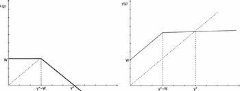
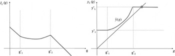
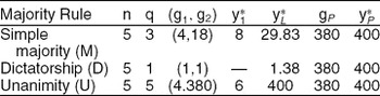
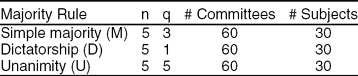
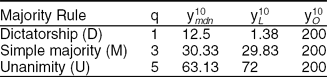

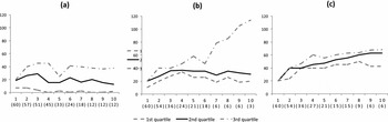
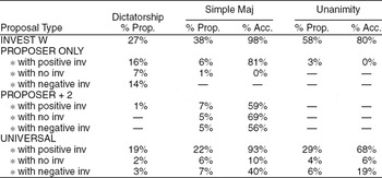
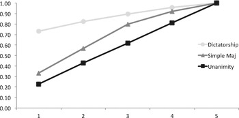
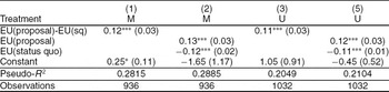
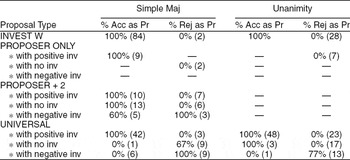
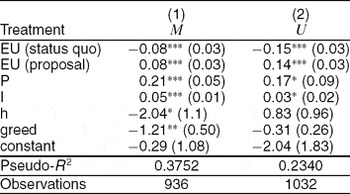
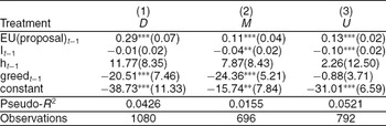




Comments
No Comments have been published for this article.