2.1. Governing Equations

In our numerical model, the plasma dynamics is described by the 3D, time-dependent ideal MHD equations in the Cartesian coordinate system, which can be written in the following form – e.g. Arber et al. (Reference Arber, Longbottom, Gerrard and Milne2001):

(1) \begin{equation} \frac{\operatorname{D}\rho}{\operatorname{D}t}=-\rho\nabla\cdot\textbf{v},\end{equation}

(2) \begin{equation} \rho\frac{\operatorname{D}\textbf{v}}{\operatorname{D}t}=-\nabla p + \textbf{j} \times \textbf{B},\end{equation}

(3) \begin{equation} \frac{\operatorname{D}\textbf{B}}{\operatorname{D}t}=(\textbf{B}\cdot\nabla)\textbf{v},\end{equation}

(4) \begin{equation} \frac{\operatorname{D}e}{\operatorname{D}t}=-\frac{p}{\rho}\nabla\cdot\textbf{v},\end{equation}

(5) \begin{equation} \nabla\cdot\textbf{B}=0,\end{equation}

where all the terms have their usual meanings. As follows from Eq. 2, gravitational acceleration is not considered in the model. Also, fully ionized plasma was considered (and therefore the adiabatic coefficient was set as $\gamma=\frac{5}{3}$ ) with an average mass of ions $1.2 m_\textrm{p}$ , typical for the solar corona.

2.2. Initial State

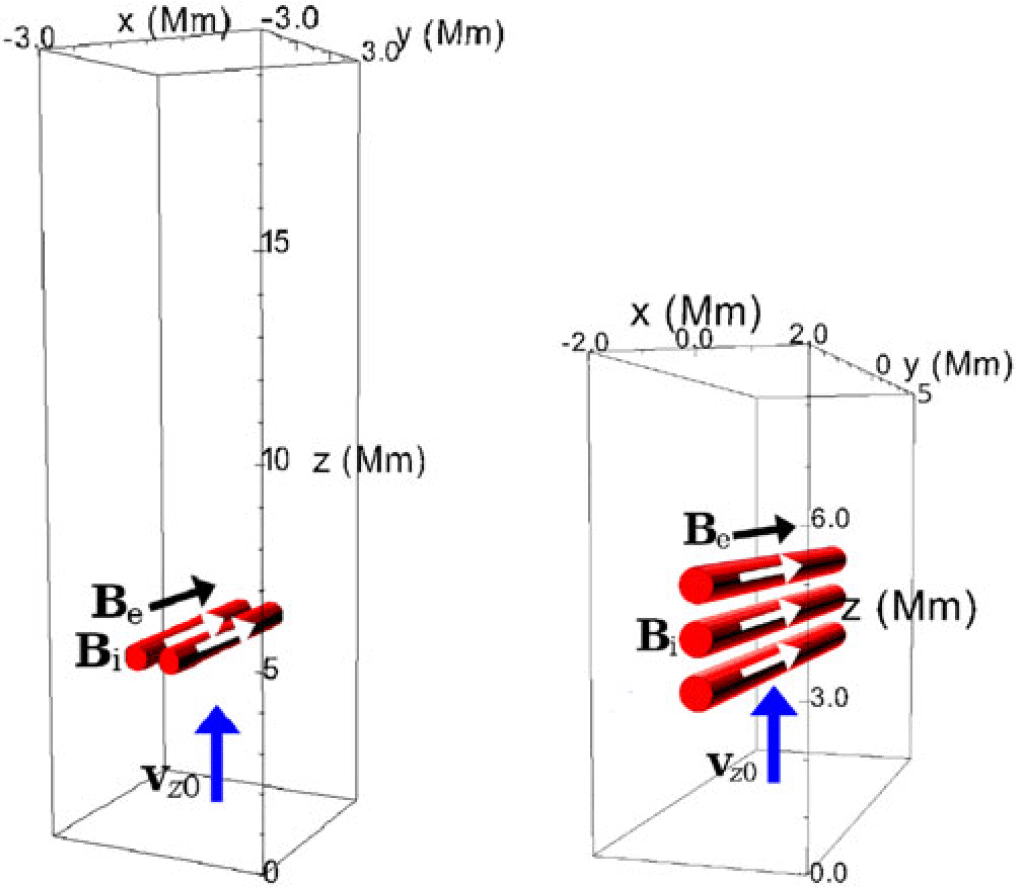
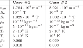
Figure 1 illustrates the simulation boxes in the initial state of each of the two studied cases (the one used for case #1 was covered by $360\times360\times1200$ grid points, i.e. its spatial resolution was 0.0167 Mm approximately; the one used for case #2 was covered by $444\times1110\times999$ grid points, i.e. its spatial resolution was 0.009 Mm approximately). The parameters set in the initial conditions of each simulation are summarized in Tab. 1. All initial parameters are set in accordance with the equilibrium condition.

Figure 1.

The sketches of the numerical boxes (not to scale) for cases #1 (left) and #2 (right) including their sizes. The red cylinders represent the obstacles. The initial flow is denoted as $\textbf{v}_{z0}$ .

Figure 1 Long description

Panel A: A 3D diagram of a numerical box with dimensions labeled in megameters (Mm) on the x, y, and z axes. The box contains a red cylinder representing an obstacle. Arrows labeled B_e, B_i, and v_z0 indicate magnetic fields and initial flow direction. Panel B: Another 3D diagram of a numerical box with different dimensions labeled in megameters (Mm) on the x, y, and z axes. This box contains multiple red cylinders representing obstacles. Arrows labeled B_o, B_i, and v_z0 indicate magnetic fields and initial flow direction.

Table 1.

Initial parameters of the studied cases.

Table 1 Long description

A table comparing initial parameters of two studied cases. The table has two columns labeled Case #1 and Case #2, and eight rows with different parameters. Row 1: v_0, 1.784 times 10^5 meters per second, 8.921 times 10^4 meters per second. Row 2: B_e, 10^-3 tesla, 10^-3 tesla. Row 3: B_i, 1.029 times 10^-3 tesla, 1.032 times 10^-3 tesla. Row 4: ρ_e, 5 times 10^-12 kilograms per cubic meter, 10^-12 kilograms per cubic meter. Row 5: ρ_i, 5 times 10^-11 kilograms per cubic meter, 10^-11 kilograms per cubic meter. Row 6: T_e, 2 times 10^5 kelvin, 10^4 kelvin. Row 7: T_i, 6 times 10^3 kelvin, 10^4 kelvin. Row 8: β_e, 0.069, 0.069. Row 9: β_i, 0.010, 0.003.

We consider two model cases: #1 – with two flexible cylindrical obstacles located next to each other with a radius square $r^2 = 0.1\;\textrm{Mm}^2$ , fixed at the boundaries, with only the y component of the magnetic field applied, with the centres 2r, 3r and 6r apart; and #2 – with the same configuration, except there are three obstacles located above each other with the centres 3r apart. There is a flow coming from the lower face of the box constantly throughout the simulations.

3.1. Flow and oscillations

Figures 2 to 3 show the distribution of the mass density in the plane $y = 0$ of cases #1 and #2. The panels are shown for different time steps.

Figure 2.

Mass density distribution in case #1 at configurations 2r, 3r and 6r respectively at different time steps indicated above. In each case, vortex shedding is taking place - see movies at QR codes. 2r: Kármán vortex street is captured; 3r: two halves of Kármán vortex streets are captured; 6r: two opposite Kármán vortex streets are captured.

Figure 2 Long description

Panel A: A heat map showing mass density distribution at t = 747.04 s. The x-axis ranges from -2 to 2 Mm and the z-axis ranges from 4 to 18 Mm. The color scale indicates the log of mass density in kg/m^3, with values ranging from -12 to -10.4. The heat map shows a concentration of higher density at the bottom center. Panel B: A heat map showing mass density distribution at t = 174.72 s. The x-axis ranges from -2 to 2 Mm and the z-axis ranges from 4 to 18 Mm. The color scale indicates the log of mass density in kg/m^3, with values ranging from -12 to -10.4. The heat map shows two symmetrical regions of higher density near the bottom center. Panel C: A heat map showing mass density distribution at t = 216.16 s. The x-axis ranges from -2 to 2 Mm and the z-axis ranges from 4 to 18 Mm. The color scale indicates the log of mass density in kg/m^3, with values ranging from -12 to -10.4. The heat map shows two symmetrical regions of higher density near the bottom center, with vortex shedding patterns visible.

In case #1, all three simulations show initial decaying oscillations in the xz plane and deformations before stabilizing (see movies linked via QR codes). In the 2r configuration (cylinders in contact), vortex shedding appears later ( $t \approx 730$ s), leading to a single Kármán vortex street and kink mode oscillations. In the 3r configuration, vortex shedding occurs earlier but does not trigger oscillations; instead, two opposing Kármán vortex street halves form due to the destructive interference of the vortices in the centre. The 6r case also shows early vortex shedding, forming two Kármán vortex streets without triggering oscillations.

In case #2, clear vertical oscillations of magnetic structures are observed in the beginning. Also, a symmetric pair of vortices forms, but the symmetry does not break, and vortex shedding does not take place.

Figure 3.

Mass density distribution in case #2 at different time steps indicated above.

3.2. Oscillation analysis

In Figs. 4–6, we approximately recorded the motion of the cylinders in the xz plane by locating the geometrical centre of the area identified as the cylinder’s transverse cross-section using the threshold method. In all #1 cases, the cylinders begin with decaying oscillations in the xz plane. The motions are slightly different but roughly symmetric within each pair. As shown in Fig. 5, z-direction oscillations are the strongest in case 3r; in the beginning, case 2r shows slightly more frequent z oscillations. Regarding the x motion (Fig. 4), the cylinder centres stabilize at a further x distance from each other compared to the initial distance; surprisingly, in the 3r configuration, the cylinders end up in the furthest position relative to the initial one; the 6r configuration leads to the most numerous oscillations in the x-direction. In case #2, a phase shift is observed between the middle and top cylinders, where the top one is ahead of the middle one (Fig. 6).

Figure 4.

Left: evolution of absolute x-position; right: evolution of relative x displacement i.e. x displacement from initial positions, for two cylinders with the centres initially separated by 2r, 3r and 6r (case #1), period values calculated by wavelet analysis (Torrence & Compo Reference Torrence and Compo1998) are indicated.

Figure 4 Long description

Three line graphs show the evolution of z position over time for two cylinders with different initial separations. Panel 2r: The graph shows the z position in millimeters on the vertical axis and time in seconds on the horizontal axis. The blue line represents the left cylinder, and the red line represents the right cylinder. Period values calculated by wavelet analysis are indicated as 45.42 seconds and 57.10 seconds. Panel 3r: The graph shows the z position in millimeters on the vertical axis and time in seconds on the horizontal axis. The blue line represents the left cylinder, and the red line represents the right cylinder. Period values calculated by wavelet analysis are indicated as 48.68 seconds. Panel 6r: The graph shows the z position in millimeters on the vertical axis and time in seconds on the horizontal axis. The blue line represents the left cylinder, and the red line represents the right cylinder. Period values calculated by wavelet analysis are indicated as 46.70 seconds.

Figure 5.

Evolution of absolute z-position for two cylinders with the centres initially separated by 2r, 3r and 6r (case #1), period values calculated by wavelet analysis (Torrence & Compo Reference Torrence and Compo1998).

Figure 6.

Left: evolution of relative z displacement i.e. z displacement from initial positions; right: evolution of absolute x-position, for three cylinders with the centres initially separated by 3r (case #2), period values calculated by wavelet analysis (Torrence & Compo Reference Torrence and Compo1998).