




No CrossRef data available.
OPTIMAL VERSUS ROBUST INFERENCE IN NEARLY INTEGRATED NON-GAUSSIAN MODELS
Published online by Cambridge University Press: 05 March 2004
Abstract
Elliott, Rothenberg, and Stock (1996, Econometrica 64, 813–836) derive a class of point-optimal unit root tests in a time series model with Gaussian errors. Other authors have proposed “robust” tests that are not optimal for any model but perform well when the error distribution has thick tails. I derive a class of point-optimal tests for models with non-Gaussian errors. When the true error distribution is known and has thick tails, the point-optimal tests are generally more powerful than the tests of Elliott et al. (1996) and also than the robust tests. However, when the true error distribution is unknown and asymmetric, the point-optimal tests can behave very badly. Thus there is a trade-off between robustness to unknown error distributions and optimality with respect to the trend coefficients.This paper could not have been written without the encouragement of Thomas Rothenberg. This is based on my dissertation, which he supervised. I also thank Don Andrews, Jack Porter, Jim Stock, and seminar participants at the University of Pennsylvania, the University of Toronto, the University of Montreal, Princeton University, and the meetings of the Econometric Society in UCLA. Comments of three anonymous referees greatly improved the exposition of the paper. I owe special thanks to Gary Chamberlain for helping me to understand these results.
Information
- Type
- Research Article
- Information
- Copyright
- © 2004 Cambridge University Press
1. INTRODUCTION
Elliott, Rothenberg, and Stock (1996) derive a class of point-optimal unit root tests in a time series model with Gaussian errors. They show that, by efficiently handling intercept and trend coefficients, their tests are generally more powerful than the standard Dickey–Fuller tests. The present paper investigates whether the same power improvements can be attained when using “robust” testing methods that are designed to improve power for non-Gaussian error distributions. I find that this improvement occurs when the true error distribution is known or at least is known to be symmetric. However, if one wants to be robust to thick-tailed, possibly asymmetric, error distributions, the power improvement found by Elliott et al. (1996) cannot be attained.
First I consider the model with an intercept and no time trend. In large samples the variation of a nearly integrated process dominates the intercept of the process. Thus the intercept can be set equal to zero when forming test statistics. The resulting point-optimal tests dominate previously proposed robust tests (see Lucas, 1995; Herce, 1996; Hasan and Koenker, 1997) which do not set the intercept to zero.
However, when the error distribution is unknown and asymmetric, setting the intercept to zero leads to a test with very bad properties. In large samples the zero-intercept tests reject a true null hypothesis with probability approaching one-half. The previously proposed inefficient tests perform well under asymmetric errors. Thus there is a trade-off between efficiently handling conditioning variables and robustness with respect to asymmetric error distributions.
Then the model with both an intercept and a linear time trend is considered and the form of the point-optimal test that is invariant to the time trend is derived. In many cases it is difficult to compute the point-optimal test, so I use Laplace's approximation to derive an asymptotically equivalent test that is easier to calculate. I show that tests based on the maximum likelihood estimator (MLE) and the likelihood ratio (LR) statistic, which were previously studied by Xiao (2001), are asymptotically admissible. When the error distribution is known and non-Gaussian, a test based on either of these statistics will in many cases have higher power than the tests suggested by Elliott et al. (1996).
In the model with a time trend, an unknown asymmetric error distribution causes the power of the point-optimal test to approach zero in large samples. The tests based on the MLE and LR statistic have slightly better properties—they have power approaching zero against local alternatives, but power approaching 1 against fixed alternatives. Thus, although asymmetric errors lead to power losses for these two procedures, the tests do not overreject a true null and are acceptable for both correctly and incorrectly specified errors. Monte Carlo results suggest the power losses are substantial for the point-optimal tests but not as bad for the MLE and LR tests.
Thus the viable unit root tests are the traditional robust tests (which inefficiently handle intercepts and trends) and the point-optimal Gaussian tests proposed in Elliott et al. (1996) (which are inefficient in the presence of thick-tailed errors). In some situations the efficiency loss due to ignoring thick-tailed errors is less than that due to inefficiently modeling the intercept and trend. For example, the point-optimal Gaussian test is more powerful than many traditional robust tests when the errors are drawn from a Student's t-distribution with five or more degrees of freedom.
Although the present paper does not specifically consider the topic, there are similar implications for the construction of confidence intervals for autoregressive roots close to one.1
Methods for constructing these intervals appear in Stock (1991), Hansen (1999), and Elliott and Stock (2001).
2. THE MODEL WITH NO TIME TREND
The observations {yt}t=1T come from the model
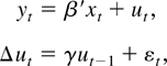
where β = (β1, β2)′ is a two-dimensional coefficient vector and xt = (1, t)′. I consider the model with an intercept only (e.g., β2 = 0) and with a linear time trend (e.g., no restrictions on β). The random errors εt are independent and identically distributed (i.i.d.) and have expectation zero and a finite variance. Under the unit root hypothesis, γ = 0, and the detrended series is not stationary. I will evaluate tests of the unit root hypothesis versus the alternatives γ < 0. Because I am interested in inference when γ is close to one, I adopt the local-to-zero reparameterization γ = c/T, so the parameter space is a shrinking neighborhood of zero as the sample size grows. Following Chan and Wei (1987) and Phillips (1987), I take c fixed when making limiting arguments, obtaining asymptotic power as a function of the local alternative c.
We distinguish between the true, unknown density for ε, given by e−f (ε), and the density used to construct the likelihood function, e−g(ε). The researcher chooses g hoping that g is a reasonable approximation to f and also hoping that the resulting tests perform well when g ≠ f. In the model with an intercept and no time trend,

is the negative of the log-likelihood function evaluated at γ = c/T, conditional on the first observation y1.
Consider the classical regression model y = α0 + α1 x + ε with nonrandom x and i.i.d. error ε. If the true value of the intercept α0 is zero, then regressing y on x alone leads to a more efficient estimator of α1 than regressing y on both x and a constant. Now consider two estimators for c.
(1)

, with a = −β1 c/T. These are the usual M-estimators studied by Lucas (1995), Hoek, Lucas, and van Dijk (1995), Herce (1996), and Hasan and Koenker (1997).
2Hasan and Koenker (1997) propose rank tests instead of M-tests. Thompson (2004) notes that under the local-to-zero reparameterization, for each rank test and error distribution there exists a test based on

with the same asymptotic power function. Thus we will not specifically discuss the rank tests.
(2)

I label this statistic the “constrained” MLE.
If β1 is zero then a is zero and

should be more efficient than

. Thus a test that rejects the null for small values of

should be more powerful than a test that rejects for small

.
We include the constant a in case β1 is not zero. However in large samples a = −β1 c/T is very close to zero no matter what the true values for β1 and c. This suggests that asymptotically it does not matter that we omit the constant. It turns out that, if g equals f (the true negative log-density of the errors), then in large samples tests based on

dominate tests based on

even when β1 and c are not zero.
This is the source of the power improvements in the model with no time trend. Many existing robust unit root tests do not take advantage of the fact that in large samples the variation in ut dominates any fixed intercept, so β1 can be taken equal to zero without affecting the asymptotic distribution of

.
We will show that in large samples, no test dominates the test based on

. This optimality result comes from the Neyman–Pearson lemma, which states that the most powerful test of c = 0 versus the alternative c = c rejects for small values of L(c, β1) − L(0, β1). In large samples, the

-test is just as powerful as the Neyman–Pearson statistic for some c. This is true even when β1 is not known.
Elliott et al. (1996) show that in a Gaussian model with an intercept and no time trend, there is no efficiency loss from β1 being unknown. The same is true for nonnormal innovations. Suppose we form the Neyman–Pearson test with an incorrect value for β1, say, 0. If g is three times differentiable with bounded second and third derivatives then by a Taylor series approximation,

where |εt* − εt| ≤ |(c − c)ut−1 /T − cβ1 /T | and |εt** − εt| ≤ |cut−1 /T |. Under regularity conditions given subsequently, ut−1 /T1/2 is Op(1). Therefore, because g′′ and g′′′ are bounded, many of the terms are asymptotically negligible:
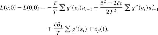
If Eg′(εt) = 0, then

, and in large samples the test statistic does not depend on β1. The term Eg′(εt) will equal zero when the errors are correctly specified, meaning that g = f:

Thus, under correct specification of the errors, there is no efficiency loss from β1 being unknown.
In a stationary autoregressive model, the Neyman–Pearson test statistic typically admits an asymptotic representation in terms of a single scalar sufficient statistic. This allows the construction of a test that is asymptotically uniformly most powerful against all alternatives c < 0. Here the Neyman–Pearson statistic has an asymptotic representation that is a linear combination of the two scalar sufficient statistics T−1 [sum ]g′(εt)ut−1 and T−2[sum ]g′′(εt)ut−12, with weights depending on c. As Elliott, Rothenberg and Stock (1996) have noted, this implies that there does not exist a uniformly most powerful test, even in large samples. Each Neyman–Pearson test is most powerful only against the point alternative c = c. The Neyman–Pearson tests comprise an infinite family of admissible tests, indexed by c, no one dominating the others for all c.
Because there is no uniformly most powerful test, the goal is to find feasible, admissible tests. Let π(c, c) denote the asymptotic power function for the Neyman–Pearson test indexed by c when the true value of the local autoregressive parameter is c and the size of the test is α:

where q(c) satisfies π(0, c) = α. Because the Neyman–Pearson test indexed by c is asymptotically optimal against the alternative c = c, the envelope power function Π(c) ≡ π(c, c) is the upper bound on power for all tests against each alternative. A test is asymptotically admissible if it has a limiting power function that is equal and tangent to the envelope function for some c.
In the next section I show that the

-test is asymptotically admissible whereas the

-test is not. There are other interesting test statistics to consider: the M-estimator t-test, which rejects for small values of

, and the constrained t and LR statistics

The

-tests impose the constraint β1 = 0, so they will dominate the M-estimator t-test.
2.1. Asymptotic Power Functions
To justify the claim that the

dominate the M-tests, it will prove convenient to develop asymptotic representations for the various statistics. Consider some of the g functions used for robust regression problems:

where the constant k is chosen by the researcher. Because g may not be everywhere differentiable, we cannot approximate the log-likelihood function with Taylor series expansions. Instead of pointwise differentiability, the proofs make use of “stochastic differentiability,” an idea described in Pollard (1985). Application of the idea requires imposition of smoothness conditions on the error density to make up for the lack of smoothness in the objective function.
Assumption 1. (Smoothness of the Error Density). The errors {εt}t=1T are i.i.d. mean zero with E|ε1|2+δ < H for some δ > 0. The term ε1 has a density function f (z) that is bounded and uniformly continuous.
The g function may have finitely many points of nondifferentiability.
Assumption 2. (Objective Function). g(x) is convex and strictly increasing in |x|, and g(x) is everywhere twice differentiable except for x in P, where P contains the D points p1,…, pD. There exists some finite positive H so that |g′′(x)| < H for x not in P. There exists some finite positive h satisfying P ∈ [−h − δ, h + δ] for some δ > 0, so that for all x and y in [−h, h] we have |g′(x)| < H and |g(x) − g(y)| ≤ H|x − y|.
I assume that g is convex because it simplifies the proofs. Assuming convexity allows me to extend several pointwise convergence results to apply uniformly over the parameter space. Convexity also greatly simplifies the demonstration of the rate of convergence of the estimators. This extensive use of convexity is due to results in Pollard (1991) and Hjort and Pollard (1993).
For nondifferentiable g, it is not possible to define an approximate likelihood in terms of the derivatives g′ and g′′. We replace g′ with the derivative-like function ψ.
DEFINITION 1. ψ(x) is equal to g′(x) if g is differentiable at x and ψ(x) = 0 otherwise.
If g is everywhere differentiable then g′ = ψ. For LAD regression ψ(x) = sign(x), and for Huber's function ψ(x) = x1(|x| < k) + k1(|x| ≥ k).
In standard (non–unit root) problems, the second derivative g′′ enters the asymptotic representation though its expectation Eg′′(ε1). We replace Eg′′(ε1) with the parameter

. When g is everywhere twice differentiable, ω = Eg′′(εt). For LAD regression ω = 2f (0), and for Huber's function ω = Pr[|x| < k] .
In large samples the power functions admit representations in terms of functionals of Brownian motion. Define W(·) to be standard Brownian motion and define Wc(·) to be the Ornstein–Uhlenbeck process

with initial condition W0(0) = 0. The asymptotic representations make use of the parameters σε2 = Var(εt), ρ = Corr(εt, ψ(εt)), and σψ2 = Var ψ(εt) and also of the stochastic process

where

is standard Brownian motion, independent of W. The following theorem is proved in Appendix A.
THEOREM 1. If Eψ(εt) = 0, and if Assumptions 1 and 2 hold, then

Rothenberg and Stock (1997) and Xiao (2001) derive similar representations without assuming convexity of g but do not allow for nondifferentiable functions.
The large sample power function for the Neyman–Pearson test is

Power functions for the other tests may be obtained similarly.
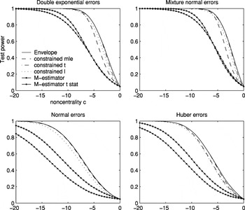
Figure 1 plots envelope power functions and asymptotic power for a variety of tests. The curves for LAD errors (from the double exponential distribution) are given and so are standard normal errors and Huber errors.3
The parameter k that appears in Huber's M function is set to 1.345 for all of the figures in this paper. At this value of k, the Huber estimate of a location parameter from i.i.d. standard normal data has a relative efficiency of 95% with respect to the mean. See Hampel, Ronchetti, Rousseeuw, and Stahel (1986, p. 399).
The log of the density for the mixture distribution is not convex. Although this violates the assumptions used to derive the asymptotic representations in Appendix B, simulations not reported here suggest that the representations are still valid.

Asymptotic power curves for unit root tests in the model with no time trend (xt = (1,0)). The curves are drawn under the assumption of correct specification, so the g function used to form the test statistics is equal to f, the negative log-density of the errors. (The simulations that appear in this paper were performed by computing stochastic integrals as the realizations of normalized sums of 500 successive draws from a discrete time Gaussian AR(1) process with autoregressive parameter 1 − c/T. There are 100,000 Monte Carlo replications.)
The power curves for nonnormal errors are all substantially higher than the curve for normal errors. The most powerful test for Gaussian errors achieves 50% power at c close to −7.0, and the most powerful test for double exponential errors (corresponding to LAD estimation under correct specification) achieves 50% power at c close to −3.75.
Figure 1 also provides power curves for the tests based on the constrained MLE

and the M-estimator

. The

-test is asymptotically admissible. Test power is tangent to the power envelope when envelope power is large. The

-test is not asymptotically admissible and is dominated by the

-test. The power curve for

touches the envelope function only under the null (c = 0) and for alternatives so far from zero that any sensible test would have power equal to 1.
The M-estimator t-test is not asymptotically admissible, whereas the constrained

-test is admissible. Figure 1 shows that the constrained t-test achieves tangency to the power envelope function at power close to 50%. The figure also shows that the constrained

-test is not admissible. As Rothenberg and Stock (1997) show, straightforward manipulations of the asymptotic representations demonstrate that rejecting for large values of

is asymptotically equivalent to rejecting for large

. Because the tests based on

are one-sided and two-sided tests of the same one-sided hypothesis, it is not surprising that the t-test dominates the test based on

.
We have obtained power improvements by imposing the constraint that the intercept estimate

is zero. We can obtain identical results by replacing the requirement that

with the requirement that the estimator

is stochastically bounded. Consider two more estimators.
(1)

, where Θ is a compact set. It is common to assume a bounded parameter space, and this estimator imposes that assumption. The estimator

is obviously stochastically bounded, and the term supβ1∈Θ|β1 c/T | disappears from the likelihood function in large samples. Thus

has the same limiting distribution as

.
(2)

. These are the MLES when we assume the initial condition u0 = 0. In an earlier draft of this paper it was shown that

is stochastically bounded. Thus

fast enough so that

has the same distribution as

.
2.2. Failure of Robustness to Error Misspecification
These power improvements occur as long as g, the estimating function, is equal to f, the true negative log-density of the errors. When g ≠ f,

may behave poorly. Consider the classical regression model y = α0 + α1 x + ε. If the errors come from the double exponential distribution, ε has zero median and the maximum likelihood estimates are the LAD estimates

. If the true value of α0 is zero, then under correct specification we can get a better estimator for α1 by removing α0 from the objective function:

. Now suppose that α0 = 0 and that ε comes from an incorrectly specified, asymmetric error distribution with zero mean but nonzero median. For example take ε = Z2 − 1 where Z is standard normal. It is well known that in this case

has a limiting distribution. It is also well known that the distribution of

is not stochastically bounded, even if α0 = 0. Thus the constant α0 “recenters” the incorrectly specified errors. In the classical setting we include the constant to protect ourselves from errors with nonzero median.
The same thing happens in the unit root problem. Herce (1996) shows that if the intercept β1 is zero and the errors have zero median, then

both have limiting distributions. When εt has a nonzero median

has a limiting distribution whereas

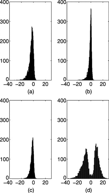
blows up. This can be seen in Figures 2a–d. Each histogram depicts 5,000 Monte Carlo realizations of

, estimated from simulated data sets of 500 observations from the model with c = 0 (so the null is true), β1 = 0 and initial condition u0 = 0. Figures 2a and b show that when the errors come from the zero median Student's t-distribution with four degrees of freedom, both estimators have limiting distributions. Figures 2c and d show that when the errors do not have zero medians (εt = Zt2 − 1 where Zt are i.i.d. standard normal) the distribution of

blows up. So for any fixed critical value q, the probability of rejecting a true null hypothesis converges to

.
Mathematically this can be understood as failure of an identification condition. Consider the classical regression model with no intercept: y = α1 x + ε. If g is differentiable, the estimator

will solve the first-order condition

. Under the usual assumptions this will deliver a consistent estimator of α1 if the identification condition Eg′(y − α1 x)x = 0 holds. Because y − α1 x = ε and x is not random, this condition is equivalent to Eg′(ε) = 0. Thus the identification condition is that ε has a distribution with the property that Eg′(ε) = 0.
In our unit root problem

solves

, which suggests the identification condition

For the LAD problem ψ(εt) = sign(εt) and the identification condition is E sign(εt) = 0. The condition holds for LAD only if the errors have zero medians.
What assumptions do we need to ensure that Eψ(εt) = 0?
(1) Expression (2) demonstrates that Eψ(εt) = 0 under correct specification (so f = g).
(2) Eψ(εt) equals zero for the Gaussian likelihood, no matter what the distribution of the errors. The Gaussian likelihood has g(x) = x2/2 and ψ(x) = x, so the assumption Eε1 = 0 insures that Eψ(ε1) = 0.
(3) Eψ(εt) equals zero when f ≠ g and both functions are symmetric around zero.
(4) When f ≠ g and f is not symmetric, Eψ(εt) can be different from zero. For example, for LAD estimation applied to the errors εt = Zt2 − 1, Eψ(εt) = E sign(Zt2 − 1) ≈ −.3656.
It turns out that the optimal tests are not robust to unknown, asymmetric error distributions. To get the tests to work, we either need to assume that we know the distribution of ε, or we need to assume that ε comes from a symmetric distribution. Thus the optimal tests are not robust to unknown asymmetric error distributions. The Gaussian tests of Elliott, Rothenberg and Stock (1996) are the one exception—those tests are valid under fairly general forms of misspecification, including asymmetric errors.
Figure 2 depicts an example where the optimal tests reject a true null hypothesis too often. This is generally a problem with asymmetric errors.

Histograms of 5,000 Monte Carlo simulations of (on the left) and (on the right) estimated from 500 observations from the model with no trend or intercept. The true value of c is 0. (a) and (b) Here the errors come from the Student's t4 distribution. Because the median is zero is more efficient and has a smaller spread around 0. (c) and (d) Here each error is εt = Zt2 − 1, where Zt are i.i.d. standard normal. Because the median is not zero, has a limiting distribution and blows up.
PROPOSITION 1. Suppose that g is three times differentiable with bounded third derivatives and suppose that the errors satisfy assumption 1. If Eψ(εt) ≠ 0 then in large samples tests based on

and the Neyman–Pearson statistic all reject a true null hypothesis with probability approaching .5, no matter what the nominal size of the test. The M-tests based on

have the same limiting representations as in Theorem 1.
5The M-tests have the same limiting representations as in Theorem 1, with the nuisance parameters σψ2, ρ, and ω replaced by Var[ψ(εt − η)], Corr[εt, ψ(εt − η)] , and

, where η denotes the parameter that solves Eψ(εt − η) = 0.
M-tests are robust to asymmetric error densities. Let η denote the parameter that solves the equation Eψ(εt − η) = 0. So for LAD estimation, ψ(εt − η) = sign(εt − η), and η is the median of the errors. The M-estimator objective function can be rewritten

with

. These recentered errors satisfy

. Thompson (2004) shows that if Eψ(εt) ≠ 0 then

in probability and

has the same limiting distribution as in Theorem 1, with a slight redefinition of the nuisance parameters (see note 5). Thus estimation of the free parameter a causes a power loss under correct specification but ensures robustness against incorrect specification.
We can avoid these centering problems by assuming that Eψ(εt) = 0. For example for LAD estimation we could assume that the median of ε is zero and leave the mean unspecified. The zero mean assumption is essential for nearly integrated models because it identifies the trend. If the mean is not zero, then the trends behave very differently under the unit root null than for stationary alternatives. Because ut follows the process Δut = γut−1 + εt, we have

with

. If γ = 0, then yt has both a unit root and a nonstochastic trend. If γ < 0, then yt is stationary with the long-run mean

. Thus the zero mean assumption is essential if we wish to test for mean reversion around an intercept. Once we assume zero means, adding additional centering assumptions such as zero medians takes us closer to assuming symmetric errors.
Sketch of proof of Proposition 1.
When Eψ(εt) ≠ 0, the Neyman–Pearson statistic is not stochastically bounded. To understand why, notice that the statistic T−1[sum ]ψ(εt)ut−1 appearing in the approximation to the Neyman–Pearson statistic is not stochastically bounded. Lemma 3.1 of Phillips (1988) implies that we must divide by T1/2 to get a limiting distribution:

where σ2(c) = (σεEψ(εt)/c)2[1 + (e2c − 1)/(2c) − 2(ec − 1)/c] . If g is three times differentiable with bounded third derivatives, the Neyman–Pearson statistic must also be divided by T1/2:
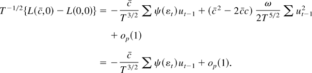
Suppose we form the Neyman–Pearson statistic and use the critical value q(c) constructed under the assumption that Eψ(εt) = 0. If Eψ(εt) ≠ 0 then under the null hypothesis the probability of rejecting is

where σ2(0) = limc→0 σ2(c) = (σεEψ(εt))2/3. In large samples the Neyman–Pearson test rejects a true null hypothesis 50% of the time, no matter what the nominal size of the test.
A proof by contradiction shows that error misspecification may also cause the constrained MLE to be stochastically unbounded. Suppose that c = β1 = 0 and g is three times differentiable with bounded third derivatives. If

is stochastically bounded, the minimized objective function admits the approximation

If

is stochastically bounded, then in large samples

must converge to the minimizer of

. The minimizer [T−2[sum ]g′′(εt)ut−12]−1T−1[sum ]ψ(εt)ut−1 is not stochastically bounded, and we have our contradiction. █
2.3. Some Monte Carlo Results
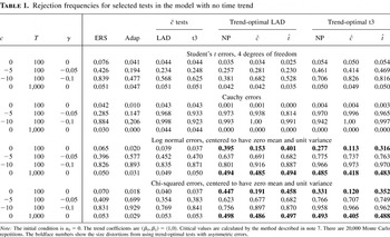
A Monte Carlo study demonstrates the size distortions that occur under incorrect specification. Table 1 presents rejection frequencies for 10 tests under various assumptions about the true data generating process. The abbreviations in the table are as follows.
(1) ERS—the Dickey–Fuller generalized least squares (DF-GLS) test of Elliott et al. (1996). This test efficiently handles the intercept for Gaussian errors but does not use the information in thick-tailed error distributions.
(2) Adap—the adaptive test of Shin and So (1999). This test adapts to the error distribution but does not efficiently handle the intercept.
(3)

test, LAD—The Thompson (2001) version of the test based on the LAD M-estimator.
6 The test is asymptotically equivalent to the test based on
and in some cases has more accurate size. This test does not efficiently handle the intercept.
(4)

test, t3—The Thompson (2001) version of the test based on the Student's t3 M-estimator.
(5) Trend-optimal LAD NP,

—these tests are optimal for a double exponential likelihood. NP denotes the Neyman–Pearson test statistic evaluated at c = −3 and β1 = 0: L(−3,0) − L(0,0). The three tests efficiently handle the trend and will be more powerful than the DF-GLS test for many thick-tailed error distributions. When the errors come from an asymmetric distribution the tests will overreject a true null hypothesis.
(6) Trend-optimal t3 NP,

—the optimal tests for a Student's t3 likelihood with β1 = 0. These tests are not robust to asymmetric errors.
Rejection frequencies for selected tests in the model with no time trend

The bold numbers in Table 1 illustrate the size problems with asymmetric errors.
7Critical values for first four tests are obtained using the methods described in Elliott et al. (1996), Shin and So (1999), and Thompson (2001). In all cases the errors are i.i.d. and no correction is made for serial correlation. Critical values for the trend-optimal tests are obtained by simulating from the asymptotic distributions in Theorem 1. The representations depend on the nuisance parameters σε, σψ, ρ, and ω. For all four tests the nuisance parameters are estimated using the formulas

, where

is a residual and ε and ψ are sample averages. For the t3 estimator ω = Eψ′(εt) is estimated by

. For the LAD test ω = 2f (η), which is estimated by the usual kernel estimator of the density of

evaluated at zero:

, where φ is the density function of a standard normal variable and h is the bandwidth

. For the Neyman–Pearson test c is not estimated and there is no residual, so we use the nuisance parameters computed for the

estimator.

-tests have accurate sizes for the asymmetric distributions.
The results demonstrate that the ERS test is a viable alternative to the robust tests even when the errors are not Gaussian. The ERS test has accurate size and good power for all four error distributions. Somewhat surprisingly, the ERS test even has accurate size for the infinite variance Cauchy distribution. The adaptive test works well for the asymmetric log normal and chi-squared distributions but has poor power for the Cauchy errors. The

-tests have accurate size for all four distributions. For the Cauchy errors the

-tests are very powerful.
3. OPTIMAL TESTS WITH A TIME TREND
If the regressors include a linear time trend,

is the log-likelihood function conditional on the first observation. Suppose we form the Neyman–Pearson statistic L(c, β1, β2) − L(0, β1, β2) with the unknown coefficients replaced by the guess b = (b1, b2)′:

In large samples the term (b1 − β1)c/T disappears from this expression, so the guess b1 does not matter. The terms (b2 − β2)(1 − (t − 1)c/T) and (b2 − β2) do not disappear, so unless we know the true β2 we cannot obtain the power bound Π(c) derived in the last section. It is important to come up with a good guess for β2.
In most situations the trend parameter β2 is unrelated to the unit root testing problem. Following Dufour and King (1991) and Elliott, Rothenberg and Stock (1996), it is natural to restrict attention to the family of tests that are invariant to the value of β2. By the well-known result of Lehmann (1959, p. 249), the most powerful invariant test of the hypothesis c = 0 versus the alternative c = c rejects for large values of

Elliott et al. (1996) encounter a similar integral for the Gaussian likelihood, where g(x) = x2/2. In the Gaussian case L(c, β1, b) is quadratic in b, and the method of “completing the square” leads to a closed-form solution for the integral. Because for many non-Gaussian likelihoods it is not obvious how to solve this integral, I approximate L(c, β1, b) with a quadratic function of b and show that the approximate solution is asymptotically equivalent to the exact solution. This approach is a variant of Laplace's method (see Judd, 1998, p. 525). Laplace uses this approach to approximate a similar integral over the double exponential distribution.8
I thank Gary Chamberlain for making me aware of the links between Laplace's integration problem and this one.
The quadratic approximation is
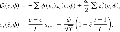

. In Lemma 1 in Appendix A, it is shown that if Eψ(εt) = 0 then

In large samples the intercept β1 disappears from the likelihood. In the proof of Theorem 2 in Appendix A it is shown that

These integrals admit analytic solutions. Tedious algebraic manipulations lead to the result that the log of this ratio is asymptotically equivalent to

plus terms that do not depend on c. This suggests the following theorem.
THEOREM 2. If Eψ(εt) = 0 and Assumptions 1 and 2 hold, the most powerful invariant test is asymptotically equivalent to the test that rejects for small values of

Let πτ(c, c) denote the limiting power function for the best invariant test indexed by c when the true value of the locally autoregressive parameter is c:

where qτ(c) satisfies πτ(0, c) = α. The most powerful invariant test against the alternative c has power equal to Πτ(c) ≡ πτ(c, c), the envelope power function.
Consider two estimators for c.
(1)

, with a1 = β2 − β1 c/T and a2 = −cβ2. These are the usual M-estimators studied by Lucas (1995), Thompson (2004), and Hasan and Koenker (1997) (see note 2).
(2)

. This estimator is suggested by Xiao (2001).
In large samples β1 c/T is close to zero. This implies that the three parameters c, a1, and a2 can be written as just two, because limT→∞ ca1 = −a2. Under correct specification of the errors,

exploits the parameter restriction and a test that rejects for small

dominates one that rejects for small

. In fact, the test based on

is asymptotically admissible, because its limiting power function touches the power envelope Πτ. The test based on

is not asymptotically admissible.
Another interesting test is the t-test based on the M-estimator, which rejects for small values of

, where

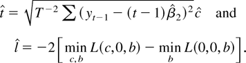
is the residual from a least squares regression of yt−1 on (1, t/T). This test is not asymptotically admissible and is dominated by the constrained t- and LR tests, which reject for small values of
3.1. Asymptotic Power Functions
To derive the power functions of the various test statistics, it will prove useful to provide a limiting representation for the objective function. By Lemma 3.1 of Phillips (1988),

where Pc, φ(r) = σε(c − c)Wc(r) + φ(1 − cr) is a stochastic process. The following theorem is proved in Appendix A.
THEOREM 3. If Eψ(εt) = 0 and Assumptions 1 and 2 hold, then

Appendix B provides a closed-form expression for

in terms of stochastic integrals. Because

is a nonlinear function of c and φ, the asymptotic representation for

does not admit an analytic solution in terms of random integrals. Appendix B provides a method for simulating from the asymptotic distribution of

.
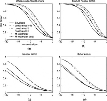
Figure 3 plots the limiting power functions for the various tests in the model with a time trend. The curves are lower than the corresponding power envelopes for the model with an intercept only. Power rises as the tails of the error distribution become thicker; for Gaussian errors 50% power is achieved at −12.5, and for double exponential errors 50% power is achieved at about −6.0.

Asymptotic power curves for unit root tests in the model with a time trend (xt = (1, t)). The curves are drawn under the assumption of correct specification, so the g function used to form the test statistics is equal to the negative log-density of the errors f. (The simulations that appear in this paper were performed by computing stochastic integrals as the realizations of normalized sums of 500 successive draws from a discrete time Gaussian AR(1) process with autoregressive parameter 1 − c/T. There are 100,000 Monte Carlo replications.)
Figure 3 shows that the constrained

-tests are asymptotically admissible. Careful examination of the figure leads to the conclusion that the constrained

-statistic is not asymptotically admissible. Neither M-test is asymptotically admissible. The

-test is point optimal when power is high, and the

-test is point optimal when power is close to one-half. Rothenberg (1984) describes similar results; he notes that in standard (non–unit root) models with no nuisance parameters, second-order asymptotic theory predicts that estimator-based tests are optimal when power is high and LR tests are optimal when power is close to 50%.
3.2. Failure of Robustness to Error Misspecification
The analysis in the previous section was carried out under the assumption of correct specification, so g = f where g is the function used to form the likelihood function and e−f is the density of εt. As discussed in Section 2.2, correct specification insures that the centering condition Eψ(εt) = 0 holds. If g ≠ f then Eψ(εt) may not equal zero. When Eψ(εt) ≠ 0 the test statistics can behave badly.
PROPOSITION 2. Suppose that g is three times differentiable with bounded third derivatives and suppose that the errors satisfy Assumption 1. If Eψ(εt) ≠ 0 then
(1) Under the local alternative

. Here

is Op(1) but does not have the distribution given in Theorem 3. Therefore power against any local alternative approaches zero.
(2) Under the fixed alternative

. Power against any fixed alternative approaches 1.
(3) If g′′(x) > B > 0 for all x, then under both local and fixed alternatives the best invariant test statistic

, where K is a compact set. Power against any fixed or local alternative approaches zero.
(4) The M-tests based on

have the same limiting distributions as in Theorem 3.
9The M-tests have the same limiting representations as in Theorem 3, with the nuisance parameters redefined as in note 5.
Because the critical values for

are always negative, tests that reject for small

will have size converging to zero and power against any local alternative also converging to zero. The

-test has power equal to size for any local alternative, and its actual size will not match its nominal size, even in large samples. Because the critical values for the best invariant test are also negative, the best invariant test has size and power approaching zero against both fixed and local alternatives. The M-tests are robust to asymmetric errors. No matter what the error distribution, the M-tests have power against local alternatives and are consistent against fixed alternatives.
Thus none of the trend-optimal tests have power against local alternatives, but all except the best invariant test have power approaching 1 against fixed alternatives. In a large sample with a local alternative, the

-tests will be dominated by the robust M-tests. Furthermore, only the M-tests are useful for forming confidence intervals for the local parameter c, because that requires inverting a sequence of tests, each with power against local alternatives (for the Gaussian case, see Elliott and Stock, 2001).
On the other hand, the

have many desirable properties even when ψ(εt) ≠ 0: in large samples they reject a true null hypothesis with probability less than any desired size, and they reject a fixed alternative γ < 0 with probability approaching 1. Although the

-test may get the size wrong, because the statistic is stochastically bounded both under the null and alternatives, the size distortions may be small. The magnitude of those distortions is evaluated by Monte Carlo in Section 3.3.
To understand the proposition, recall that the M-estimators

minimize the objective function

where

denotes the parameter that solves Eψ(εt − η) = 0. If the condition Eψ(εt) = 0 fails to hold then
, and the “recentered” errors

satisfy

. Thus

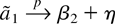
has the same limiting distribution as in Theorem 3, with a slight redefinition of the nuisance parameters (see note 5). This result is shown by Thompson (2004), and it implies that statement 4 of the proposition will hold. Because there is no free “recentering” parameter in the objective function for

, the parameter on the time trend accomplishes the recentering. If

, no matter what the local alternative c.
Sketch of proof of Proposition 2.
To establish statement 1 of the proposition, consider the model with the local alternative γ = c/T. Define φ = (φ1, φ2)′ = (T1/2c,T1/2(b2 − β2 − η))′ and mt = T−1/2(−η(t − 1)/T,1)′. The likelihood function is

A Taylor series expansion, combined with the usual asymptotic arguments (see Phillips, 1988, Lemma 3.1), implies that

where

for any compact set K. By the same argument used to prove Lemma 2, φ is stochastically bounded. Therefore, by the argmax continuous mapping theorem of Wellner (1996, p. 286),

converges in probability to the minimizer of the approximating quadratic function, so

Here [sum ] mt mt′ converges in probability to a nonrandom matrix, and

converges to a vector of mean zero Gaussian random variables. In large samples

has a mean zero Gaussian distribution, which implies that

.
The distribution of

is obtained by substituting

back into the likelihood function. Under the local alternative γ = c/T, we obtain

This is an Op(1) variable, but the limiting distribution differs from the one in Theorem 1.
Statement 2 of the proposition says that the

-tests are consistent against any fixed alternative γ < 0. The likelihood function evaluated at (γ, b) may be written

Because ut−1 is stationary under the fixed alternative, is it straightforward to show using Taylor series–based arguments that

is consistent for γ. Therefore

, and an argument based on a Taylor series expansion demonstrates that

. The proofs are omitted to save space.
To show statement 3 of the proposition, define the parameter ηγ that satisfies Eψ(εt + γut−1 − ηγ) = 0. For fixed γ < 0, εt + γut−1 is a stationary random variable, and the expectation exists. By a Taylor series expansion,
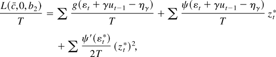
where zt* = −cut−1 /T − β1 c/T + ηγ − (b2 − β2)(1 − c((t − 1))/T) and |εt* + γut−1 − ηγ| ≤ |zt*|. If b2 ∈ K then many of the terms are asymptotically negligible. We get the approximation
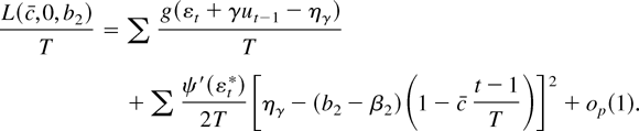
If c = 0 this expression is minimized at b2 = β2 + ηγ, so minb∈K T−1L(0,0, b) = T−1[sum ]g(εt + γut−1 − ηγ) + op(1). If c ≠ 0, then because g′′(x) ≥ B we have

Therefore T−1{minb∈K L(c,0, b2) − minb∈K L(c,0, b2)} ≥ (24)−2Bηγ2 c2 + op(1), and the best invariant test converges to +∞ under any fixed alternative. Using the same arguments it is also possible to show that the best invariant test converges to +∞ under any local value γ = c/T (including the null c = 0). The proof is omitted to save space. █
3.3. Some Monte Carlo Results
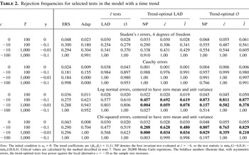
Table 2 presents rejection frequencies for various tests in the model with a time trend. The tests are the trend versions of the tests that appeared in Table 1, except that the

-test appears in Table 2 in place of the

-test. This substitution was made because the

-test is not asymptotically admissible in the model with a time trend.
10As was the case for Table 1, the

tests are the Thompson (2001) versions of the tests. In the model with a time trend the test rejects for small values of

, where rt is the residual from a least squares regression of yt−1 on (1, t) and

with

. Thompson (2001) shows that

.
Rejection frequencies for selected tests in the model with a time trend

The power losses from using the trend-optimal

-tests are small for samples of 100 observations but get larger for samples of 1,000. For the asymmetric log normal and chi-squared error distributions, power against the local alternative c = −10 declines as sample size grows. Power against the fixed alternative γ = −0.1 increases with sample size. This can be seen by comparing the results for the samples with (T, c) = (100,−10) against the samples with (T, c) = (1,000,−100). In each case γ = −0.1. These results are consistent with Proposition 2, which states that power against c = −10 converges to zero as the sample grows and power against γ = −0.1 converges to 1.
In the samples of 1,000 observations, asymmetric errors cause the NP test to have low power against both the fixed and local alternatives. This is consistent with Proposition 2, which predicts that power against both kinds of alternatives converges to zero as the sample size grows.
No test dominates the others. The ERS test performs poorly for the Cauchy, log normal, and chi-squared errors. The adaptive test does well for the asymmetric distributions but has very low power with Cauchy errors. The
-tests perform well for all the error distributions and sample sizes but are generally dominated by the trend-optimal

-tests for samples of 100.
APPENDIX A: PROOFS
In this Appendix we prove Theorems 1–3. Throughout the Appendix it will prove useful to make use of the normalized likelihood

. The remainder term RT(c, b1, φ) is defined to be the difference between

and its quadratic approximation


Preliminary Lemmas
LEMMA 1. Let K denote a compact set. If Eψ(εt) = 0, and if Assumptions 1 and 2 hold, then

.
We will show that

pointwise in (c, b1, φ). If

were a convex function of (c, b1, φ) then pointwise convergence would imply uniform convergence over compact sets (this is shown in Hjort and Pollard, 1993, Lemma 1). However, even though g(x) is convex in x,

is not a convex function of (c, b1, φ) because g(εt + (b1 − β1)c/T − zt(c, φ)) is a nonlinear function of the parameters.
A reparameterization allows us to restore the link between pointwise and uniform convergence. Let wt = T−1/2(T−1/2,T−1/2ut−1,1,(t − 1)/T)′ and θ = (θ1, θ2, θ3, θ4)′ = (c(β1 − b1), c − c, φ,−φc)′. We have the reparameterized objective function and remainder term
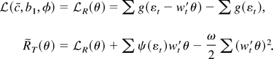
Because g is convex and εt − wt′θ is a linear function of

is a convex function of θ. Therefore if

pointwise in θ then the convergence is uniform for θ in a compact set. The relationship between the original remainder term and the reparameterized remainder is

The equality holds as long as θ satisfies the constraint θ4 = −θ3(θ2 + c). For any compact set

, let

denote a compact set large enough so that if {θ1, θ2, θ3} ∈ K then

. We now have a bound for the remainder RT:
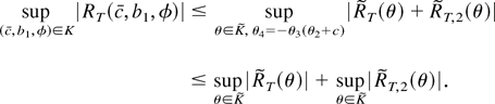
It is straightforward to show that

in probability for any compact set

. So to prove the theorem it is enough to show that

pointwise in θ. The pointwise convergence of

was proved in Lemma 1 of Thompson (2004). █
LEMMA 2. In the model with a time trend, define

and

. If Eψ(εt) = 0, and if Assumptions 1 and 2 hold, then

are both stochastically bounded.
If

were convex in the parameters the argument in Section 3 of Pollard (1991) could be used to show that the estimators

are stochastically bounded. However, even though g(x) is convex in

is not a convex function of (c, φ) because g(εt − β1 c/T − zt(c, φ)) is a nonlinear function of the parameters. We will pursue a related method of proof.
A reparameterization allows us to apply the arguments of Pollard (1991) to this problem. Define θ = (c − c, φ + β1 c/T, −φc)′, wt = T−1/2(T−1/2ut−1, 1, (t − 1)/T)′, and

Note that this reparameterization differs from the reparameterization in Lemma 1 because here we take b1 = 0. For some k > 0, define the compact set K = {(c, φ) : |c − c| < k, |φ + T−1/2β1 c| < k}. For any (c, φ) ∉ K, the corresponding θ vector is equal to vr where v is a vector with unit length and r is a scalar with r > k. Because g is convex and εt − wt′θ is a linear function of θ,

is a convex function of θ. So k = (1 − λ)0 + λr for λ = k/r, and by the convexity of

,

which implies that

. In the proof of Lemma 1 it was found that the approximation

will hold uniformly over θ in a compact set. So for fixed k,

By Lemma 3.1 of Phillips (1988),[sum ]wt wt′ converges in distribution to a positive definite matrix with diagonal elements bounded away from zero with probability one. Therefore there exists ε > 0 so that inf∥v∥=1 v′([sum ]wt wt′)v > ε. So

Because ∥[sum ]wtψ(εt)∥ is stochastically bounded (see Phillips, 1988, Lemma 3.1), we can choose k large enough so that k2ωε/2 − k∥[sum ]wtψ(εt)∥ > ε with probability arbitrarily close to 1. We have that in large samples,

So in large samples the estimators

must be contained in K. Thus

are stochastically bounded, and the theorem is proved. █
Proofs of Theorems
Proof of Theorem 1. Notice that

and that

. By Lemma 1,

The asymptotic representation for L(c,0) − L(0,0) follows from the following weak convergence result, which was proved by Phillips (1988, see Lemma 3.1):

Because g is convex,

is convex in c. By slightly modifying the argument in Section 3 of Pollard (1991), it can be shown that the convexity of

implies that

converges weakly to the minimizer of the quadratic approximation

, so

Therefore

, and the distribution of

follows similarly. The representations for

are provided in Theorem 1 of Thompson (2004). █
Proof of Theorem 2. To prove the theorem it is sufficient to show that

To see that this is indeed sufficient, notice that the best invariant test rejects for large values of

where the last equality follows from the change of variables

. The discussion in Section 3 indicates that if the approximation in (A.1) holds, then the best invariant test is asymptotically equivalent to rejecting for small values of

This is asymptotically equivalent to minb L(c,0, b) − minb L(0,0, b). To see this, notice that

The convexity of g implies that for fixed c,

is convex in φ. By slightly modifying the method in Section 3 of Pollard (1991), one can use the convexity to show that

is asymptotically equal to

, the quadratic approximation given in Lemma 1. So in large samples

is equivalent to the statistic in (A.2). Thus verifying the condition in (A.1) is sufficient to prove the theorem.
To verify (A.1) it will prove convenient to break the integral into two parts. For any positive k,

with

. For any fixed k, Lemma 1 implies that

The integral on the right-hand side admits an analytic solution. Using that analytic solution it is straightforward to show that for all ε > 0 we can pick k large enough so that

It remains to show that

is asymptotically negligible. Because

is convex in φ (for fixed c), then if φ > k then k = (1 − λ)0 + λφ and

with λ = k/φ. Therefore

Similarly,

By Lemma 1, for fixed k we have

By the usual asymptotic arguments, limT→∞ T−1[sum ](1 − c(t − 1)/T)2 = c2/3 − c + 1 ≥ ¼, and the other terms are Op(1). So if |φ| > k then

Plugging this bound into the integral, we obtain

Thus, for any ε > 0, we can choose k large enough so that

. Thus the condition in (A.1) holds, and the theorem is proved. █
Proof of Theorem 3. In the proof of Theorem 2, we showed that

Lemma 3.1 of Phillips (1988) implies that

. Lemma 3.1 of Phillips (1988) also implies that

is stochastically bounded, and

by the argmax continuous mapping theorem of Wellner (1996, p. 286). We have derived the limiting representation for the best invariant test.
The argmax continuous mapping theorem also provides the limiting result for

. Notice that

. Because by Lemma 2

are stochastically bounded,

converge weakly to

. The limiting distributions of

follow from a similar argument.
Limiting representations for

are provided in Theorem 1 of Thompson (2004). █
APPENDIX B: SIMULATING THE ASYMPTOTIC DISTRIBUTIONS
Theorem 3 provides asymptotic representations for various test statistics in the model with a time trend. In this Appendix we describe how to simulate from those distributions.
The best invariant test converges to

. This is equal to

Simulating from this distribution is straightforward.
The normalized MLEs

converge weakly to the random variables

that minimize the stochastic objective function

. I was unable to derive a simple expression for

. Instead the variables are expressed implicitly as solutions to the minimization problem. Rewrite the objective function:

where λ = ωσε /σψ and

The expression

has at least one minimum. Take the derivatives of the function with respect to

:

The values of

that minimize

set the partial derivatives to zero. Solve

to obtain
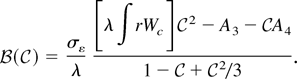
Substitute the solution for

into the equation

to show that

is the root of a fifth-order polynomial:

Notice that because A0, A1, A3, and A4 depend on ρ and λ and on no other nuisance parameters, the distribution of

depends only on ρ and λ.
There is no known closed-form solution for the root of a general fifth-order polynomial. Simulation was done from the asymptotic distribution for

by the following method. Simulate a draw from the joint distribution of the five coefficients of the polynomial. Use a software package (Matlab version 5.3 was used here) to numerically calculate the roots of the resulting polynomial. The real root

that maximizes

is the simulated draw from the asymptotic distribution of

. The corresponding draw from the asymptotic distribution of the t-statistic is

The stochastic integrals were computed as the realizations of normalized sums of 500 successive draws from a discrete time Gaussian AR(1) process with autoregressive parameter 1 − c/500.
The simulation procedure was repeated 100,000 times for each value of λ, ρ, and c. The asymptotic critical value for a size 100α% test that rejects for small

was calculated as the 100,000αth element of the vector of sorted draws for

. The power of the test at the alternative c was calculated as the proportion of draws below the critical value. A similar procedure was used to calculate the critical value and power of the test based on the t-statistic.
References
REFERENCES
Chan, N.H. &
C.Z. Wei
(1987)
Asymptotic inference for nearly nonstationary AR(1) processes.
Annals of Statistics
15,
1050–1063.CrossRefGoogle Scholar
Dufour, J.M. &
M.L. King
(1991)
Optimal invariant tests for the autocorrelation coefficient in
linear regressions with stationary or nonstationary AR(1) errors.
Journal of Econometrics
47,
115–143.CrossRefGoogle Scholar
Elliott, G.,
T. Rothenberg, &
J.H. Stock
(1996)
Efficient tests for an autoregressive unit root.
Econometrica
64,
813–836.CrossRefGoogle Scholar
Elliott, G. &
J.H. Stock
(2001)
Confidence intervals for autoregressive coefficients near one.
Journal of Econometrics
103,
155–181.CrossRefGoogle Scholar
Hampel, F.R.,
E.M. Ronchetti,
P.J. Rousseeuw, &
W.A. Stahel
(1986)
Robust statistics: The approach based on influence functions.
Wiley.
Hansen, B.E.
(1999)
The grid bootstrap and the autoregressive model.
Review of Economics and Statistics
81,
594–607.CrossRefGoogle Scholar
Hasan, M.N. &
R.W. Koenker
(1997)
Robust rank tests of the unit root hypothesis.
Econometrica
65,
133–161.CrossRefGoogle Scholar
Herce, M.A.
(1966)
Asymptotic theory of LAD estimation in a unit root process with
finite variance errors.
Econometric Theory
12,
129–153.Google Scholar
Hjort, H.L. &
D. Pollard
(1993) Asymptotics for Minimizers of Convex Processes. Preprints, Department of Statistics, Yale University.
Hoek, H.,
A. Lucas, &
H.K. van Dijk
(1995)
Classical and Bayesian aspects of robust unit root inference.
Journal of Econometrics
69,
27–59.CrossRefGoogle Scholar
Judd, K.L.
(1998)
Numerical Methods in Economics.
MIT Press.
Lehmann, E.L.
(1959)
Testing Statistical Hypotheses.
Wiley.
Lucas, A.
(1995)
Unit root tests based on m estimators.
Econometric Theory
11,
331–346.CrossRefGoogle Scholar
Phillips, P.C.B.
(1987) Toward a unified asymptotic theory for autoregression.
Biometrika 74
535–547.CrossRef
Phillips, P.C.B.
(1988)
Regression theory for near-integrated time series.
Econometrica
56,
1021–1043.CrossRefGoogle Scholar
Pollard, D.
(1985)
New ways to prove central limit theorems.
Econometric Theory
1,
295–314.CrossRefGoogle Scholar
Pollard, D.
(1991)
Asymptotics for least absolute deviation regression estimators.
Econometric Theory
7,
186–199.CrossRefGoogle Scholar
Rothenberg, T.J.
(1984)
Approximating the distributions of econometric estimators and test
statistics. In
Z. Griliches &
M. Intriligator (eds.),
Handbook of Econometrics,
vol. 2.
North-Holland.
Rothenberg, T.J. &
J.H. Stock
(1997)
Inference in a nearly integrated autoregressive model with
nonnormal innovations.
Journal of Econometrics
80,
269–286.CrossRefGoogle Scholar
Shin, D.W. &
B.S. So
(1999)
Unit root tests based on adaptive maximum likelihood estimation.
Econometric Theory
15,
1–23.CrossRefGoogle Scholar
Stock, J.H.
(1991)
Confidence intervals for the largest autoregressive root in U.S.
macroeconomic time series.
Journal of Monetary Economics
28,
435–459.Google Scholar
Thompson, S.B.
(2001) Robust Confidence Intervals for Autoregressive Coefficients near One. Working paper, Harvard University.
Thompson, S.B.
(2004) Robust tests of the unit root hypothesis should not be ‘modified.’
Econometric Theory.
van der Vaart, A.W. &
J.A. Wellner
(1996)
Weak Convergence and Empirical Processes.
Springer-Verlag.
Xiao, Z.
(2001)
Likelihood-based inference in trending time series with a root near
unity.
Econometric Theory
17,
1082–1112.Google Scholar
Asymptotic power curves for unit root tests in the model with no time trend (xt = (1,0)). The curves are drawn under the assumption of correct specification, so the g function used to form the test statistics is equal to f, the negative log-density of the errors. (The simulations that appear in this paper were performed by computing stochastic integrals as the realizations of normalized sums of 500 successive draws from a discrete time Gaussian AR(1) process with autoregressive parameter 1 − c/T. There are 100,000 Monte Carlo replications.)
Histograms of 5,000 Monte Carlo simulations of (on the left) and (on the right) estimated from 500 observations from the model with no trend or intercept. The true value of c is 0. (a) and (b) Here the errors come from the Student's t4 distribution. Because the median is zero is more efficient and has a smaller spread around 0. (c) and (d) Here each error is εt = Zt2 − 1, where Zt are i.i.d. standard normal. Because the median is not zero, has a limiting distribution and blows up.
Rejection frequencies for selected tests in the model with no time trend
Asymptotic power curves for unit root tests in the model with a time trend (xt = (1, t)). The curves are drawn under the assumption of correct specification, so the g function used to form the test statistics is equal to the negative log-density of the errors f. (The simulations that appear in this paper were performed by computing stochastic integrals as the realizations of normalized sums of 500 successive draws from a discrete time Gaussian AR(1) process with autoregressive parameter 1 − c/T. There are 100,000 Monte Carlo replications.)
Rejection frequencies for selected tests in the model with a time trend
 You have
Access
- 6
- Cited by