





1 Introduction
Detecting incorrect program behaviors during the compilation phase is an important and complex part of the software development cycle. With the advent of machine-generated code, and as more non-experts are able to write complex software, ensuring that semi-automatically generated programs behave as expected has become increasingly important. To aid in this process, a number of tools have been developed to compare actual program behavior against expectations, such as code analyzers/verifiers and run-time verification frameworks. These tools rely on language-level constructs to describe expected program behavior. Approaches that fall into this category include assertion-based frameworks used in (Constraint) Logic Programming ((C)LP) (Drabent et al. Reference Drabent, Nadjm-Tehrani and Małuszyński1988; Puebla et al. Reference Puebla, Bueno and Hermenegildo1997; Bueno et al. Reference Bueno, Deransart, Drabent, Ferrand, Hermenegildo, Maluszynski and Puebla1997; Boye et al. Reference Boye, Drabent and Małuszyński1997; Hermenegildo et al. Reference Hermenegildo, Puebla and Bueno1999; Laï Reference Laï2000; Puebla et al. Reference Puebla, Bueno and Hermenegildo2000b; Hermenegildo et al. Reference Hermenegildo, Puebla, Bueno and Garcia2005; Mera et al. Reference Mera, Lopez-Garcia and Hermenegildo2009; Hanus Reference Hanus2017), soft/gradual typing approaches in functional programming (Cartwright and Fagan Reference Cartwright and Fagan1991; Findler and Felleisen Reference Findler and Felleisen2002; Tobin-Hochstadt and Felleisen Reference Tobin-Hochstadt and Felleisen2008; Dimoulas and Felleisen Reference Dimoulas and Felleisen2011; Rastogi et al. Reference Rastogi, Swamy, Fournet, Bierman and Vekris2015; Takikawa et al. Reference Takikawa, Feltey, Dean, Flatt, Findler, Tobin-Hochstadt and Felleisen2015, Reference Takikawa, Feltey, Greenman, New, Vitek and Felleisen2016; Vazou et al. Reference Vazou, Tanter and Horn2018) and contract-based extensions in object-oriented programming (Lamport and Paulson Reference Lamport and Paulson1999; Leavens et al. Reference Leavens, Leino and Müller2007; Fähndrich and Logozzo Reference Fähndrich and Logozzo2011). These approaches often involve a certain degree of run-time testing, especially for non-trivial properties. However, such testing can incur significant performance overhead (Mera et al. Reference Mera, Lopez-Garcia and Hermenegildo2009), even when performing simple type checks between typed and untyped parts of programs (Rastogi et al. Reference Rastogi, Swamy, Fournet, Bierman and Vekris2015; Takikawa et al. Reference Takikawa, Feltey, Greenman, New, Vitek and Felleisen2016).
Some proposals have been made to reduce the run-time overhead of assertion checking by optimizing the run-time checking mechanisms themselves, at the expense of increased memory consumption (Koukoutos and Kuncak Reference Koukoutos and Kuncak2014; Stulova et al. Reference Stulova, Morales and Hermenegildo2015). Repeated checks on immutable recursive data structures are converted from execution-time overhead into increased memory use via caching and/or tabling techniques. Despite these advances, full run-time checking often remains impractically expensive, especially for complex properties such as deep data structure tests. This reduces the attractiveness of run-time checking to programmers, who may allow sporadic checking of very simple conditions but tend to disable run-time checking for more complex properties. Motivated by this problem, assertion-based frameworks have been proposed in which static analysis is used to reduce the number of program points where run-time checks are required, or to rule out incorrect program behaviors (Puebla et al. Reference Puebla, Bueno and Hermenegildo1997; Bueno et al. Reference Bueno, Deransart, Drabent, Ferrand, Hermenegildo, Maluszynski and Puebla1997; Hermenegildo et al. Reference Hermenegildo, Puebla and Bueno1999). A number of practical assertion checking modes have been studied, representing different trade-offs between code annotation depth, execution-time slowdown, and program behavior safety guarantees (Stulova et al. Reference Stulova, Morales and Hermenegildo2018). The latter proposed a method to modify the semantics inferred by the analyzer via program transformations to capture executions with active run-time checking. While this technique had limitations, it showed the potential to increase the number of checks verified at compile time.
In this work, we take a complementary approach by incorporating the run-time checking semantics directly into the analyzer, but making it optional, allowing abstract executions to more closely match their concrete counterparts. By making the presence or absence of run-time checks part of the analyzed semantics, the analyzer can reason precisely about program executions under different assertion checking configurations. We also study the effect of multivariant analysis in this setting, which makes it possible to distinguish between different calling contexts and different versions of the same predicate or procedure, depending on the properties known to hold and on whether run-time checks are required. Multivariant analysis is particularly well suited to (C)LP, where predicates are naturally invoked under different modes of use. If such modes are not taken into account, the analysis is forced to merge distinct execution contexts, often leading to a loss of precision and overly conservative decisions regarding run-time checking. By explicitly representing different analysis versions corresponding to different calling modes and run-time checking configurations, we study how making these versions explicit can improve analysis precision and run-time checking efficiency. Finally, beyond measuring how many assertions are completely verified, as is common practice, we also evaluate whether individual properties within an assertion are checked. Note that assertions often consist of multiple properties of varying complexity: for example, in a formula such as
 $(\mathit{simple\_property}(X), \mathit{complex\_property}(Y), \mathit{less\_complex\_property}(Z))$
, some properties (such as
 $\mathit{simple\_property(X)}$
) may be fully verified statically, others (
 $\mathit{complex\_property}(Y)$
) may never be discharged, and yet others (
 $\mathit{less\_complex\_property}(Z)$
) may be verified only under certain calling contexts. We aim to capture this finer-grained information, allowing us to quantify how many properties of each assertion are verified, under which conditions, and how many remaining properties require run-time checking, with special attention to multivariance.
2 Preliminaries and notation
Variables start with a capital letter. The set of terms is inductively defined as follows: (1) variables are terms (2) if
 $f$
is an
 $n$
-ary function symbol and
 $t_{1},\ldots , t_{n}$
are terms, then
 $f({t_{1},\ldots , t_{n}})$
is a term. An atom has the form
 $p({t_{1},\ldots , t_{n}})$
where
 $p$
is an
 $n$
-ary predicate symbol, and
 $t_{1},\ldots , t_{n}$
are terms. A constraint is a conjunction of expressions built from predefined predicates whose arguments are constructed using predefined functions and variables, for example,
 $X-Y \gt \text{ abs}(Z)$
. A literal is either an atom or a constraint. We denote the set of variables of a literal
 $L$
by
 $\mathsf{vars}(L)$
. Negation is encoded as finite failure, supported through a program expansion. A goal is a finite sequence of literals. A rule has the form
 $H\,\texttt {:-}\,B$
where
 $H$
, the head, is an atom and
 $B$
, the body, is a possibly empty finite sequence of literals. A predicate is a set of rules with the same head. We refer to a predicate by either its function symbol and arity
 $p/n$
, or its head
 $p({t_{1},\ldots , t_{n}})$
. A constraint logic program, or program, is a finite set of rules. For simplicity, we assume a single program
 $\mathcal{P}$
in which every rule has distinct variables in its head; and a class of constraints – over a given constraint domain – for which projection and a complete solver exist.
Operational semantics.
The operational semantics, adapted from that of Jaffar et al. (Reference Jaffar, Maher, Marriott and Stuckey1998), is given in terms of derivations from goals. Derivations are sequences of reductions between states. A state
 $\langle G\, |\, \theta \rangle$
consists of a goal
 $G$
, and the current constraint
 $\theta$
. We denote sequence concatenation by (::). We use
 $\leadsto S'$
to indicate that a reduction step can be applied to state
 $S$
to obtain state
 $S'$
. And
 $S\leadsto ^{*} S'$
to indicate that there exists a sequence of reduction steps from
 $S$
to
 $S'$
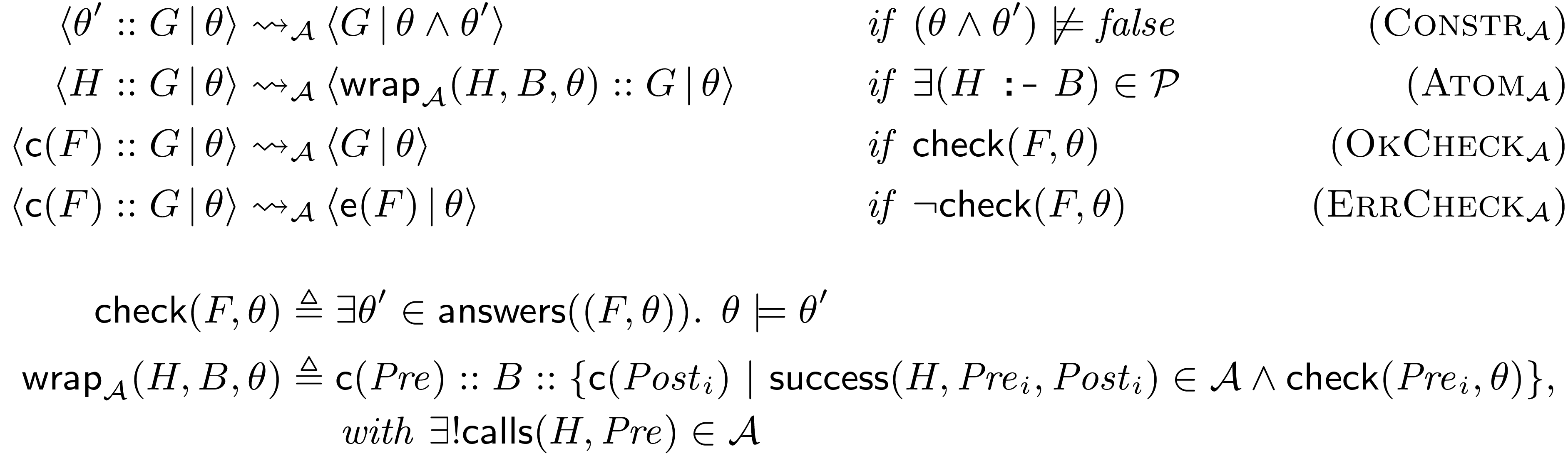
. Figure 1 depicts the reduction rules. Intuitively, satisfiable constraints are added to the current constraint (Constr), and atoms are reduced by unfolding them into the bodies of matching program rules (Atom).
Reduction rules for the operational semantics of (C)LP programs.

Given a literal
 $L$
and reduction steps
 $S\leadsto ^{*} S'$
from state
 $S = \langle L::G\, |\, \theta \rangle$
to state
 $S' = \langle G\, |\, \theta ' \rangle$
, we refer to
 $S$
as a call state for
 $L$
, and to
 $S'$
as a success state for
 $L$
.
A query is a pair
 $(L,\theta )$
, where
 $L$
is a literal and
 $\theta$
is a constraint for which the (C)LP system starts a computation from state
 $\langle L\, |\, \theta \rangle$
. A finite derivation from a query
 $Q=(L,\theta )$
is finished if the last state in the derivation cannot be reduced. Such a finished derivation is successful if the last state is of the form
 $\langle \square \, |\, \theta ' \rangle$
, where
 $\square$
denotes the empty goal sequence, and the projection of the constraint
 $\theta '$
onto the variables
 $\mathsf{vars}(L)$
is an answer to
 $Q$
. Conversely, a derivation is failed if the last state is not of the form
 $\langle \square \, |\, \theta \rangle$
. We denote by
 $\mathsf{answers}(Q)$
the set of answers to the query
 $Q$
.
Properties & property formulas. Conditions on the current constraint are stated as property formulas, which are conjunctions of properties. Properties are predicates, typically defined in the source language, and thus runnable. However, not all predicates can be used as properties. They are generally required to be checkable at run time so that they can be effectively used as run-time checks, but not necessarily decidable at compile time, where they can be safely approximated (Hermenegildo et al. Reference Hermenegildo, Puebla and Bueno1999; Puebla et al. Reference Puebla, Bueno and Hermenegildo2000b).
Example 2.1 (Properties)
The following are the definitions of the
 $\mathit{list/2}$
,
 $\mathit{tree/2}$
and
 $\mathit{list\_or\_tree/2}$
properties:

Note that all definitions are
 $\mathrm{parametric}$
on an additional property (their first argument), which is then called using higher-order notation (
P(X)
).
Assertions. Assertions are syntactic objects which allow expressing properties of programs that must be satisfied at certain points of program execution. We recall the relevant parts of the assertion schema of Puebla et al. (Reference Puebla, Bueno and Hermenegildo2000a). Predicate (or pred) assertions have the following syntax:

where
 $\text{ Pred}$
is an atom representing a predicate, and
 $\text{ Pre}$
and
 $\text{ Post}$
are property formulas. They express that all calls to
 $\text{ Pred}$
must satisfy the pre-condition
 $\text{ Pre}$
, and, if such calls succeed, the postcondition
 $\text{ Post}$
must be satisfied. If there are several pred assertions, the
 $\text{ Pre}$
field of at least one of them must be satisfied. To simplify both presentation and use, assertions are normalized into a set of corresponding assertion conditions.
Definition 2.1 (Assertion conditions)
Given a predicate
 $\text{ Pred}$
and its corresponding set of assertions
 $\{{A_{1},\ldots , A_{n}}\}$
with
 , its set of
 $\mathrm{assertion\, conditions}$
is defined as
 $\{C_0,{C_{1},\ldots , C_{n}}\}$
with:
 \begin{equation*} C_i = \begin{cases} \mathsf{calls}(\text{ Pred},\bigvee _{j=1}^n\, \text{ Pre}_j) & i = 0\\ \mathsf{success}(\text{ Pred},\text{ Pre}_i,\text{ Post}_i) & i \in \{1, \ldots , n\} \end{cases}\\ \end{equation*}
 $C_0$
encodes the checks that the calls to the predicate represented by
 $Pred$
are within those admissible by the set of assertions. We refer to it as the
 $\text{calls assertion condition}$
.
 $C_{1},\ldots , C_{n}$
encode the checks for compliance of the success states for particular sets of calls, and we call them the
 $\text{success assertion conditions}$
.
We denote by
 $\mathcal{A}$
both the set of assertions of the program and, interchangeably, its associated set of assertion conditions. And we assume that, if there are no assertions associated with a predicate
 $\text{ Pred}$
, its set of assertion conditions is defined as
 $\{\mathsf{calls}(\text{ Pred},\text{ true}),\mathsf{success}(\text{ Pred},\text{ true},\text{ true})\}$
; that is, the most-general assertion/assertion conditions.
Example 2.2 (Member program with assertions)
Consider the program in Figure
2
, which defines the predicate
 $\mathit{member(X,S)}$
, relating a number
 $X$
with a structure
 $S$
. As specified by its assertion, it succeeds when the number
 $X$
occurs at some position in the structure
 $S$
, where
 $S$
may be a
 $\mathrm{list}$
or a
 $\mathrm{binary\, tree}$
.
An example Prolog program with an assertion capturing its behavior.

Run-time assertion checking. Run-time assertion checking consists of dynamically checking that the conditions imposed by the assertions hold while computing the derivations from a query. To this end, we incorporate instrumental checks into the operational semantics in Figure 1.
We extend the set of literals with additional syntactic objects: check literals of the form
 $\mathsf{c}(F)$
, where
 $F$
is a property formula to be checked at run-time; and error literals of the form
 $\mathsf{e}(F)$
, where
 $F$
is a property formula that has been violated.
Reduction rules for the operational semantics of (C)LP programs with assertions.

We use
 $S\leadsto _{\mathcal{A}} S'$
to indicate run-time checking reductions w.r.t. a set of assertions
 $\mathcal{A}$
. Figure 3 depicts the reduction rules and some auxiliary functions. Intuitively, atoms are still reduced by unfolding them into the bodies of matching program rules. However, the body is now preceded by a run-time check for the predicate’s pre-condition, that is, its calls assertion condition, and followed by a sequence of run-time checks for the predicate’s applicable post-conditions, that is, its set of success assertion conditions whose pre-condition held at the atom’s call state (Atom
 $_{\mathcal{A}}$
). Run-time checks are computed by means of the
 $\mathsf{check}$
function, which determines whether a property formula
 $F$
holds under the current constraint
 $\theta$
by searching for a solution for
 $F$
that is entailed by
 $\theta$
. Since run-time checks may fail, we introduce the notion of (finite) erroneous derivations, whose final state is of the form
 $\langle \mathsf{e}(F)\, |\, \theta \rangle$
indicating that the run-time check of
 $F$
under
 $\theta$
was false (ErrCheck
 $_{\mathcal{A}}$
).
While useful, run-time assertion checking can be prohibitively expensive in both time and memory. Consider calling the
 $\mathit{member/2}$
predicate in Example 2.2 with the calling mode expressed by
 . Then, checking that
 $S$
is a list at each recursive step turns the
 $\mathcal{O}(n)$
algorithm into
 $\mathcal{O}(n^2)$
.
Abstract interpretation.
The main idea behind abstract interpretation (Cousot and Cousot Reference Cousot and Cousot1977) is to interpret the program over a special, abstract domain whose elements are finite representations of possibly infinite sets of states in the concrete domain. We denote the concrete domain as
 $D_{\gamma }$
, the abstract domain as
 $D_{\alpha }$
, and the functions that relate sets of states with their abstractions as the abstraction function
 $\alpha : D_{\gamma } \rightarrow D_{\alpha }$
and the concretization function
 $\gamma : D_{\alpha } \rightarrow D_{\gamma }$
. The concrete domain is typically a complete lattice with the set inclusion order which induces an ordering relation in the abstract domain represented by
 $\sqsubseteq$
. Under this relation the abstract domain is usually a complete lattice and
 $(D_{\gamma }, \alpha , D_{\alpha }, \gamma )$
is a Galois insertion/connection (Cousot and Cousot Reference Cousot and Cousot1977).
Top-down analyses are a family of static analyses that build an analysis graph starting from a series of program entry points. This approach was first used in analyzers such as MA3 and Ms (Warren et al. Reference Warren, Hermenegildo and Debray1988), and matured in the PLAI analyzer (Muthukumar and Hermenegildo Reference Muthukumar and Hermenegildo1990, Reference Muthukumar and Hermenegildo1992) using an optimized fixpoint algorithm now also referred to as the top-down algorithm or solver. This algorithm was later applied to the analysis of CLP/CHCs (de la Banda et al. Reference de la Banda, Hermenegildo, Bruynooghe, Dumortier, Janssens and Simoens1996)Footnote
1
and imperative programs (Henriksen and Gallagher Reference Henriksen and Gallagher2006; De Angelis et al. Reference De Angelis, Fioravanti, Gallagher, Hermenegildo, Pettorossi and Proietti2021; Méndez-Lojo et al. Reference Méndez-Lojo, Navas and Hermenegildo2007a, Reference Méndez-Lojo, Navas and Hermenegildo2007b), and used in analyzers such as GAIA (Le Charlier and Van Hentenryck Reference Le Charlier and Van Hentenryck1994), the CLP(
 $\mathcal R$
) analyzer (Kelly et al. Reference Kelly, Marriott, Søndergaard and Stuckey1998), or Goblint (Seidl and Vogler Reference Seidl and Vogler2021; Tilscher et al. Reference Tilscher, Stade, Schwarz, Vogler and Seidl2023). The graph constructed by the PLAI algorithm during analysis is a finite, abstract object whose concretization approximates the (possibly infinite) set of (possibly infinite) maximal and-trees of the concrete semantics. This follows the overall abstraction scheme of Bruynooghe (Reference Bruynooghe1991), but implementing it with an efficient fixpoint algorithm that uses tabling, dependency-based acceleration, incrementality, etc. PLAI separates the abstraction of the structure of the concrete trees (the paths through the program) from the abstraction of the constraints at the nodes in those concrete trees (the program states in those paths). The first abstraction,
 $T_{\alpha }$
, is typically built-in, as an abstract domain of analysis graphs. The framework is parametric on a second abstract domain,
 $D_{\alpha }$
, whose elements appear as labels in the nodes of the analysis graph. Each node of the analysis graph is of the form
 $\langle \lambda ^c,H,\lambda ^s \rangle$
with
 $H$
a call pattern for a predicate of the program and
 $\lambda ^c$
and
 $\lambda ^s$
the abstractions of the call and success states.
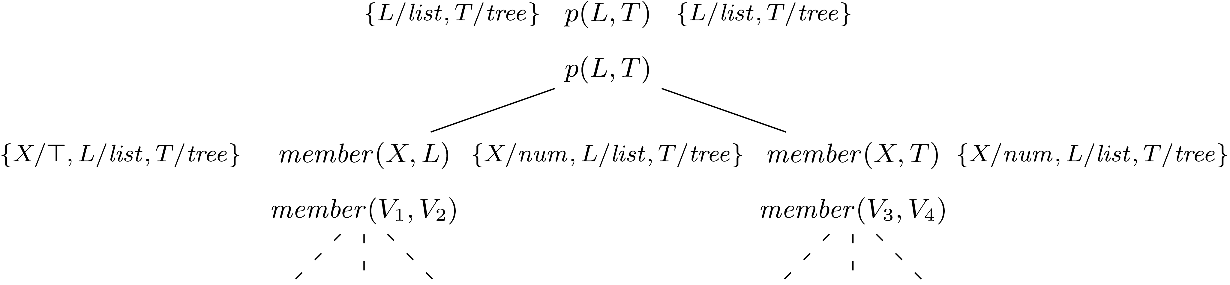
Multivariance and path sensitivity. The abstract semantics computed by PLAI is multivariant. That is, for a single program point, it computes separate path information for each of its calling contexts (also referred to as variants, versions or modes). In the analysis graph, this is represented by multiple nodes corresponding to the same program point, each abstracting a different calling mode.
Example 2.3 (Analysis)
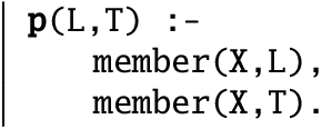
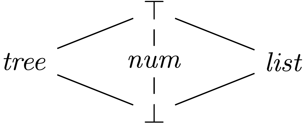
Consider the simple abstract domain depicted in Figure
6
. Figure
4
shows a (partial) analysis graph for the program in Figure
5
. Notice that the success abstraction of member
 $(X,L)$
becomes the call abstraction of member
 $(X,T)$
. Notice also how two different versions for
 $\mathit{member/2}$
do appear, with (abstract) call patterns
 $\{X/\top ,L/\text{ list},T/\text{ tree}\}$
and
 $\{X/\text{ num},L/\text{ list},T/\text{ tree}\}$
, respectively.


Program with different calling modes.

Abstract domain lattice.

Compile-time assertion verification & simplification.
Compile-time assertion verification consists of statically checking that the conditions imposed by the assertions hold for all possible derivations of a program from a set of queries. This verification can be performed using the analysis graph computed by PLAI, which is an over-approximation of the program’s semantics for all such derivations. However, since PLAI is multivariant, a single program point
 $H$
may correspond to multiple nodes in the analysis graph:
 $ \langle \lambda ^c_1,H,\lambda ^s_1 \rangle , \ldots , \langle \lambda ^c_n,H,\lambda ^s_n \rangle ,$
with each node over-approximating the semantics of that point for some derivations. Consequently, the over-approximation of the semantics of a program point for all derivations is the combination (lub) of all corresponding nodes in the analysis graph:
 $ \langle \sqcup \{\lambda ^c_1,\ldots ,\lambda ^c_n\},$
H,
 $\sqcup \{\lambda ^s_1,\ldots ,\lambda ^s_n\} \rangle .$
This can then be used for simplifying (as much as possible) the property formulas in the corresponding assertion conditions. That is, given a program point and its abstraction, properties implied by the abstraction simplify to
 $\text{ true}$
, properties incompatible with it simplify to
 $\text{ false}$
, while the remaining ones remain unchanged. This approach has the advantage that, even if a property formula cannot be proved in its entirety – given the undecidable nature of (non-trivial) semantic properties – it may be possible to discharge some parts of it. The verification results are reported as changes in the status and transformations of the assertions. An assertion is checked if both property formulas are simplified to
 $\text{ true}$
, and false if some property formula is simplified to
 $\text{ false}$
. If some property formula cannot be fully proved, the assertion is check, and its property formulas are replaced with their simplified versions.
From this point on, we assume that the program
 $\mathcal{P}$
, the set of assertions
 $\mathcal{A}$
and the analysis graph
 $\mathcal{G}$
are implicit variables.
3 Assertion checking with abstract run-time checking semantics
The operational semantics of (C)LP with run-time assertion checking (cf. Figure 3) differs from the default (C)LP semantics (cf. Figure 1) in that the latter can be seen as an over-approximation of the former. Intuitively, run-time assertion checking may cause certain program points to become unreachable due to failing checks, whereas they would be reachable under the default semantics. As a result, for a given program
 $\mathcal{P}$
, the set of and-trees generated under the default (C)LP semantics is a superset of those generated when run-time assertion checking is enabled. Thus, abstract interpretation analyses based on the default semantics are correct but may suffer from a loss of precision, since they abstract a set of and-trees that over-approximates the actual execution space. In contrast, analyzing programs under run-time checking semantics allows us to exploit the additional information provided by assertions. Concretely, when entering a predicate definition, we may assume that the corresponding calls assertion condition holds and thus enrich the call abstraction
 $\lambda ^c$
with this information. Similarly, upon predicate exit, we can assume that the relevant success assertion conditions hold and use them to refine the resulting success abstraction
 $\lambda ^s$
.
Stulova et al. (Reference Stulova, Morales and Hermenegildo2018) propose a program transformation based on the introduction of additional link predicates with assertions that enriches the analysis with the run-time checking semantics. In contrast, in this work we focus on integrating run-time checking semantics directly into the top-down abstract interpretation framework without transforming the original program. However, since the information in the assertions is now included in the abstractions, those abstractions would trivially satisfy the assertions they are intended to check, turning the analysis results unsuitable for assertion checking. To address this, we generate alternative call and success abstractions at those program points where the assertions’ information causes a gain in precision and use these during the (abstract) assertion checking phase to ensure correct behavior. We now describe this technique in detail.
Assertion-based abstraction refinement.
Assume a literal
 $L$
in the body of some clause in the program, and a rule
 $H\,\texttt {:-}\,B$
s.t.
 $H$
unifies with
 $L$
. Assume also that the constraint affecting
 $L$
at the time of this call is approximated by the abstraction
 $\lambda ^c$
such that
 $\mathsf{vars}(L)\subseteq \mathsf{dom}(\lambda ^c)$
and
 $\mathsf{vars}(\lambda ^c)\cap (\mathsf{vars}(H)\cup \mathsf{vars}(B))=\varnothing$
. The success (exit state) of
 $L$
after executing the rule above is represented by the abstraction
 $\lambda ^s$
given by:
 \begin{align*} \lambda ^s &= \mathsf{extend}(\lambda ^c,L,\lambda ^p_{rt}) \\ \lambda ^p_{rt}&=\mathsf{absAssrtPrimes}(\lambda ^{pr}_{rt},\lambda ^p_{},L) \\ \lambda ^p_{} &= \mathsf{exitToPrime}(\mathsf{project}(\mathsf{vars}(H), \lambda ^{ex}), H, L) \\ \lambda ^{ex} &= \mathsf{entryToExit}(\lambda ^{en}, H, B) \\ \lambda ^{en} &= \mathsf{augment}(\mathsf{vars}(B)\backslash \mathsf{vars}(H), \mathsf{callToEntry}(\lambda ^{pr}_{rt}, L, H)) \\ \lambda ^{pr}_{rt}&=\mathsf{absAssrtProjs}(\lambda ^{pr},L) \\ \lambda ^{pr} &= \mathsf{project}(\mathsf{vars}(L), \lambda ^c) \end{align*}
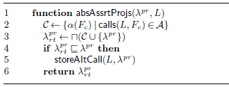
absAssrtProjs function.

Algorithm 1 Long description
An equation describing a function named absAssrtProjs with input parameters lambda P T and L. The function begins by assigning the set C as the intersection of alpha open parenthesis F C close parenthesis and calls open parenthesis L, F C close parenthesis is an element of A. Lambda P T T is then assigned the union of C and the set open parenthesis lambda P T close parenthesis. A conditional statement checks if lambda P T is an element of lambda P T T. If true, it stores altCall open parenthesis L lambda close parenthesis. The function returns lambda P T T.
The analyzer operates as follows: (1) First, it projects the call abstraction (
 $\lambda ^c$
) over the variables in the literal (
 $L$
). (2) The computed
 $\lambda ^{pr}$
assertion is then enriched by incorporating the glb (
 $\sqcap$
) of the assertion pre-conditions for the predicate of
 $L$
. This is achieved by invoking the
 $\mathsf{absAssrtProjs}$
(Algorithm1). If the resulting abstraction is more precise than the initial
 $\lambda ^{pr}$
, an alternative call abstraction is stored for use during the assertion checking phase (Algorithm1, lines 4–6). (3) Next, it performs abstract unification using the
 $\mathsf{callToEntry}$
function. (4) The resulting abstraction is then augmented with any variables in the body not present in the head. (5) The clause body is then traversed, and each literal is analyzed using the
 $\mathsf{entryToExit}$
function, producing an exit abstraction (
 $\lambda ^{ex}$
). (6) The abstract unification from step (2) is reverted via
 $\mathsf{exitToPrime}$
, yielding a prime abstraction (
 $\lambda ^p_{}$
). (7) This abstraction is then enriched with the applicable assertion post-conditions by computing
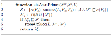
 $\mathsf{absAssrtPrimes}$
(Algorithm2). As in step (2), if the abstraction obtained is more precise than the initial one, an alternative success abstraction is stored (Algorithm2, lines 4–6). (8) Finally, this abstraction is incorporated into the original call, returning the success abstraction (
 $\lambda ^s$
) through the
 $\mathsf{extend}$
function.
As some final remarks, if no predicate head can be unified with the literal under analysis, a bottom abstraction (
 $\bot$
) is returned (representing that the exit state is unreachable). If several clauses are available, all of them are analyzed, and a collection of prime abstractions
 $\lambda ^p_{1},\ldots ,\lambda ^p_{m}$
is obtained, one abstraction per clause, where
 $m$
is the number of clauses. Then, the success abstraction is computed as
 $\lambda ^s = \mathsf{extend}(\lambda ^c,\sqcup \{\lambda ^p_{1},\ldots ,\lambda ^p_{m}\})$
by means of the lub of the collection of abstractions (other operators, including disjunction and widenings, are possible).
absAssrtPrimes function.

Algorithm 2 Long description
The table outlines a function named absAssrtPrimes with specific steps and conditions. It includes a series of steps from 1 to 6, each describing a part of the function’s operation. The steps involve projections, enrichments, abstractions, and checks. The table uses mathematical notations and logical operators to describe the processes. Each step is followed by a condition or action, such as storing alternative abstractions or returning specific abstractions.
4 Exploiting versions for more optimization
By default, after computing the analysis graph, PLAI produces an output that is easy for the programmer to inspect, that is, close to the source program, where the abstract semantics of each predicate is the combination of all its versions. That is, for a predicate
 $\text{ Pred}$
, the multiple nodes
 $\{ \langle \lambda ^c_1,\text{ Pred},\lambda ^s_1 \rangle , \ldots , \langle \lambda ^c_n,\text{ Pred},\lambda ^s_n \rangle \}$
in the analysis graph corresponding to the different calling modes of
 $\text{ Pred}$
, are collapsed into a single node
 $\langle \sqcup \{\lambda ^c_1,\ldots ,\lambda ^c_n\}, \text{ Pred}, \sqcup \{\lambda ^s_1,\ldots ,\lambda ^s_n\} \rangle .$
This approach, while convenient for the end-user, may incur a significant loss of precision, not due to the analysis itself, but rather to the over-simplification of the abstractions. To address this issue, PLAI is also capable of producing an output where multiple versions of each original predicate
 $\text{ Pred}$
, that is, multiple nodes for
 $\text{ Pred}$
, are materialized into different predicates which, through a program transformation, are “folded back” to the program. That is, for a predicate
 $\text{ Pred}$
, the multiple nodes:
 $\{ \langle \lambda ^c_1,\text{ Pred},\lambda ^s_1 \rangle , \ldots , \langle \lambda ^c_n,\text{ Pred},\lambda ^s_n \rangle \}$
in the analysis graph corresponding to the different calling modes of
 $\text{ Pred}$
are materialized into different predicates for each version:
 $\{ \langle \lambda ^c_1,\text{ Pred}_1,\lambda ^s_1 \rangle , \ldots , \langle \lambda ^c_n,\text{ Pred}_n,\lambda ^s_n \rangle \}.$
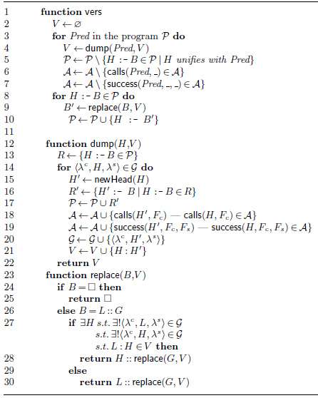
vers program transformation.

Algorithm 3 Long description
The image displays a code listing for a program transformation algorithm named ‘vers’. The code is structured into three main functions: ‘vers’, ‘dump’, and ‘replace’. The ‘vers’ function initializes an empty set V and iterates over predicates in the program P. It calls the ‘dump’ function and updates sets A and P based on predicate calls and successes. The ‘dump’ function processes a head H and body B of a clause, creating new heads and updating sets R, P, A, and G. The ‘replace’ function handles the replacement of variables in a body B with values from a set V. Each function is defined with specific steps and conditions, involving set operations and unification processes.
A high-level view of the program transformation is depicted in Algorithm3. For each predicate in the program, we first dump its versions (line 4). That is, for each version of a predicate in the analysis graph (line 14), a copy is created by generating a new head (line 15) and attaching to it the corresponding rules (line 16), assertions (lines 18–19), and analysis graph node (line 20), updating the program, assertion set, and analysis graph accordingly. Additionally, a versions mapping
 $V$
is created in order to record which versions correspond to the original predicates (line 21). Then, each rule in the program is rewritten by replacing calls to the original predicates, under a specific calling mode, with calls to the corresponding specialized predicates generated by
 $\mathsf{dump}$
(lines 9 and 10). Concretely, during the traversal of a rule’s body, any literal corresponding to a predicate call for which a specialized version exists for the given call pattern is replaced by a call to that specialized version (line 27).
Example 4.1 (Exploiting versions)
Applying the
 $\mathsf{vers}$
transformation to the program in Figure
2
(with the analysis information of the
 $\mathrm{Eterms}$
abstract domain (Vaucheret and Bueno, Reference Vaucheret and Bueno2002)) generates two versions of the predicate for its possible abstract call patterns (
 $\mathit{member\_1/2}$
and
 $\mathit{member\_2/2}$
):

For instance, for the analysis version with calling abstraction
 $\{X/\text{ term}, L/\text{ list}(\text{ num})\}$
, the
 $\mathit{member\_2/2}$
version with success abstraction
 $\{X/\text{ num}, L/\text{ rt1}\}$
is created.

The obtained success abstraction is
 $\mathrm{strictly\, more\, precise}$
than that obtained by analyzing the program in Figure
2
with the
 $\mathrm{Eterms}$
abstract domain. Therefore, all assertions proven to be checked in the original program remain checked.

However, without versioning, recursive calls to
 $\mathit{member/2}$
must be checked at run time. In contrast, with versions, recursive calls are directed to the specialized predicate version, for which the assertions have already been statically verified. As a result, additional run-time checks are unnecessary.
5 Experimental evaluation
In order to assess the benefits of the proposed techniques, we evaluate two sets of benchmarks. These benchmarks include a variety of examples, ranging from a collection of classic benchmarks for Prolog to a subset of libraries of the Ciao system. While the predicates in the first set often have a single assertion per predicate, those in the second set typically present more assertions per definition, describing several possible call patterns. Our objective is to measure the effects of applying different techniques for the optimization of run-time checks. To this end, instead of measuring the number of assertions that are completely checked, that is, those that are reduced to
 $true$
, we count the number of properties that are simplified within the assertions. We use this metric because assertions can sometimes contain one or more properties that are hard to verify, while other properties in the assertion are verified. The metric chosen allows us to measure the effects of different techniques at a finer level of granularity. Then, we also evaluate the impact of these techniques on the execution times of the programs when executed under run-time checking semantics. The experiments were run on a MacBook Air with the Apple M1 chip and 16 GB of RAM, with a per-run timeout of 3 minutes.
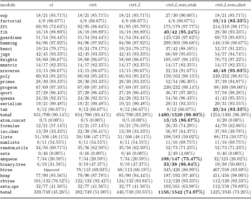
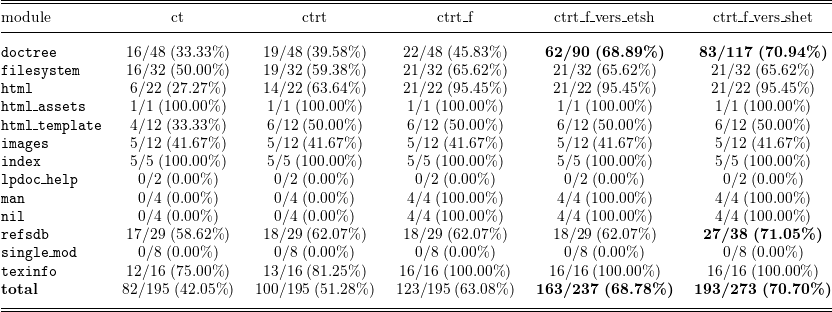
Table 1 presents the results of the first evaluation. Each column displays the number of properties actually verified (“checked”) at compile time, the total number of properties in the corresponding module, and the percentage of properties checked. These experiments use the Eterms and Sharing-Freeness abstract domains. Column ct presents results when using the information obtained from the classic fixpoint with default semantics. Column ctrt_f shows results when executing the fixpoint with run-time checking semantics, as defined in Section 3. Column ctrt_f_vers_etsh (resp. ctrt_f_vers_shet) displays results when executing the fixpoint with run-time checking semantics, followed by the versions transformation (i.e., materializing the versions contained in the multivariant information of Eterms), and then analyzing these using Sharing-Freeness (resp. with the multivariant information of Sharing-Freeness and analyzing using Eterms). A domain combination approach can be used to join versions but we wanted to observe the effects of the versions of each domain separately. The results show that applying run-time checking semantics to the analyzer increases the number of verified properties. The transformation obviously raises the total property count (since assertions are duplicated across versions), but the usage of multivariant information yields overall better percentages. Notably, different modules show varied improvements based on whether the multivariant information inferred from Sharing-Freeness or Eterms is used for the versions transformation.
Number of reduced properties (%)

Table 1. Long description
The table presents the results of the first evaluation, comparing the number of properties verified at compile time across different modules and conditions. It includes columns for different conditions: ct, ctrt, ctrt_f, ctrt_f_vers_etsh, and ctrt_f_vers_shet. Each row represents a different module, and the values indicate the number of properties verified and the total number of properties, along with the percentage of properties checked. The table is structured with column headers and row labels, providing a detailed comparison of the effectiveness of different abstract domains and transformations. Panel A: The table includes columns for ct, ctrt, ctrt_f, ctrt_f_vers_etsh, and ctrt_f_vers_shet, each representing different conditions. The row labels indicate different modules. Each cell contains values for the number of properties verified, the total number of properties, and the percentage of properties checked. Notable trends include varied improvements in the number of verified properties based on the use of multivariant information from Sharing-Freeness or Eterms. Panel B: The table continues with more modules and their respective values under different conditions. The data shows that applying run-time checking semantics increases the number of verified properties, and the transformation raises the total property count, but the usage of multivariant information yields better percentages. Panel C: The table concludes with the total values for each condition, summarizing the overall effectiveness of the different approaches. The results highlight the impact of using multivariant information on the verification of properties.
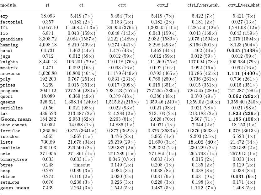
Execution time, ms (speed-up w.r.t. rt)

Table 2. Long description
The table presents performance metrics for various modules, including their run times and comparisons across different conditions. The table has 38 rows and 8 columns. Column headers are module, rt, ct, ctrt, ctrt_f, ctrt_f_vers_etsh, and ctrt_f_vers_sheet. Row labels are exp, factorial, fft, fib, guardians, hamming, hanoi, jugs, knights, mmatrix, nreverse, poly, primes, progeom, qsort, queens, serializelist, tak, Geom. mean, atom_concat, formulae, iso_char, lists, numlists, sets, binary_tree, btree, heap, rbtre, sets_ops, and geom. mean. Each row lists the performance metrics for a specific module. For example, the row for exp shows rt as 38.093, ct as 5.419 (7x), ctrt as 5.454 (7x), ctrt_f as 5.419 (7x), ctrt_f_vers_etsh as 5.422 (7x), and ctrt_f_vers_sheet as 5.421 (7x). The table provides a detailed comparison of how each module performs under different conditions.
Table 2 presents the execution times for the programs, running with run-time checks activated, for the different techniques. As a baseline, column rt shows the execution times without any optimization. We also show in parenthesis the speed-ups obtained with respect to our baseline.
The results indicate that applying any of the proposed techniques significantly improves program execution times. The fixpoint analysis with run-time semantics yields results similar to those obtained with the transformation technique proposed by Stulova et al. (Reference Stulova, Morales and Hermenegildo2018). In a few cases, however, the ctrt technique outperforms our fixpoint implementation (e.g., fft). This difference is caused by the widening operators in the Eterms abstract domain being overly conservative very soon in the fixpoint iteration. In that example, only one property was not checked under the ctrt transformation, yet this caused the fixpoint approach to be 32 times slower. Even so, it remained 12 times faster than the baseline. This example highlights the importance of discharging as many properties as possible at compile-time. It also raises questions about whether additional improvements, or new widening operators are needed, and whether more precise operations could further improve execution times. Exploiting the multivariant information to automatically generate program versions allows speed-ups of up to
 $118\times$
compared to the ctrt transformation (e.g., tak). In some cases, this corresponds to a total speed-up of up to
 $240\times$
with respect to the baseline (rt) execution. Unlike ctrt, which requires manually crafting specialized versions, the new technique materializes versions systematically. This is especially relevant in more realistic modules, where multiple assertions and call patterns would make a manual, per-predicate specialization impractical. For programs where more moderate speed-ups were observed (ranging from
 $2\times$
to
 $10\times$
), execution times were comparable to the more precise approach. In all cases, both techniques were still several times, or even orders of magnitude, faster than the baseline execution. We also observe that the order in which the information of the versions from different domains is applied matters, as expected (e.g., factorial, nreverse, qsort, and tak, vs., e.g., atom_concat, iso_char, or lists). In practice we would thus use a combined domain approach, or simply try both orders and keep the best.
As a final experiment, we tested the approach on a more complex application: the LPdoc documenter (Hermenegildo Reference Hermenegildo2000; Hermenegildo and Morales Reference Hermenegildo and Morales2011). LPdoc is a documentation generator for LP systems, used in both Ciao and XSB. In addition to generating all the Ciao system manuals and XSB manuals, it is used to generate many websites, class slides and exercises, user program documentation, etc. It comprises approximately 22K lines of Prolog code, plus the use of many Ciao libraries. The results on property reduction are shown in Table 3. Perhaps the most notable (and encouraging) conclusion from this experiment is that these results do not differ qualitatively from those on the smaller benchmarks, and similar positive overall patterns are observed. Overall, the ctrt_f_vers_shet analysis verified 193 properties out of a total of 273, that is, 70% of all the properties appearing in the assertions in the code. Furthermore, the verification process detected some errors in LPdoc that had gone unnoticed for many years.
Number of reduced properties (%) for LPdoc

Table 3. Long description
The table presents the number of reduced properties for LPdoc across different modules. It has 10 rows and 6 columns. The columns are labeled ct, ctrt, ctrt_f, ctrt_f_vers_etsh, and ctrt_f_vers_shet. The rows are labeled with different modules: doctree, filesystem, html, html_assets, html_template, images, index, lpdoc_help, man, nil, refsdb, single_mod, and texinfo. The total row sums up the values for each column. Here are the values row-wise: Row 1: doctree, 16/48 (33.33 percent), 19/48 (39.58 percent), 22/48 (45.83 percent), 62/90 (68.89 percent), 83/117 (70.94 percent). Row 2: filesystem, 16/32 (50.00 percent), 19/32 (59.38 percent), 21/32 (65.62 percent), 21/32 (65.62 percent), 21/32 (65.62 percent). Row 3: html, 6/22 (27.27 percent), 14/22 (63.64 percent), 21/22 (95.45 percent), 21/22 (95.45 percent), 21/22 (95.45 percent). Row 4: html_assets, 1/1 (100.00 percent), 1/1 (100.00 percent), 1/1 (100.00 percent), 1/1 (100.00 percent), 1/1 (100.00 percent). Row 5: html_template, 4/12 (33.33 percent), 6/12 (50.00 percent), 6/12 (50.00 percent), 6/12 (50.00 percent), 6/12 (50.00 percent). Row 6: images, 5/12 (41.67 percent), 5/12 (41.67 percent), 5/12 (41.67 percent), 5/12 (41.67 percent), 5/12 (41.67 percent). Row 7: index, 5/5 (100.00 percent), 5/5 (100.00 percent), 5/5 (100.00 percent), 5/5 (100.00 percent), 5/5 (100.00 percent). Row 8: lpdoc_help, 0/2 (0.00 percent), 0/2 (0.00 percent), 4/4 (100.00 percent), 4/4 (100.00 percent), 4/4 (100.00 percent). Row 9: man, 0/4 (0.00 percent), 0/4 (0.00 percent), 4/4 (100.00 percent), 4/4 (100.00 percent), 4/4 (100.00 percent). Row 10: nil, 0/4 (0.00 percent), 0/4 (0.00 percent), 4/4 (100.00 percent), 4/4 (100.00 percent), 4/4 (100.00 percent). Row 11: refsdb, 17/29 (58.62 percent), 18/29 (62.07 percent), 18/29 (62.07 percent), 18/29 (62.07 percent), 27/38 (71.05 percent). Row 12: single_mod, 0/8 (0.00 percent), 0/8 (0.00 percent), 0/8 (0.00 percent), 0/8 (0.00 percent), 0/8 (0.00 percent). Row 13: texinfo, 12/16 (75.00 percent), 13/16 (81.25 percent), 16/16 (100.00 percent), 16/16 (100.00 percent), 16/16 (100.00 percent). Row 14: total, 82/195 (42.05 percent), 100/195 (51.28 percent), 123/195 (63.08 percent), 163/237 (68.78 percent), 193/273 (70.70 percent).
6 Related approaches
The pattern of folding assertion pre-conditions into a multivariant abstract state and discharging post-conditions per clause appears, at least partially, in other approaches. Perhaps the closest to the CiaoPP model (Hermenegildo et al. Reference Hermenegildo, Puebla and Bueno1999) is soft contract verification in higher-order functional languages (Nguyen et al. Reference Nguyen, Tobin-Hochstadt and Van Horn2014, Reference Nguyen, Gilray, Tobin-Hochstadt and Van Horn2017), as well as the gradual-typing-optimization line (Rastogi et al. Reference Rastogi, Swamy, Fournet, Bierman and Vekris2015; Takikawa et al. Reference Takikawa, Feltey, Greenman, New, Vitek and Felleisen2016), which has also aimed in part at generating residual programs with optimized run-time checks. Also related, but not necessarily aimed at producing optimized programs, are assume-based imperative abstract interpreters such as Astrée (Cousot et al. Reference Cousot, Cousot, Feret, Mauborgne, Miné, Monniaux and Rival2005), Frama-C/EVA (Kirchner et al. Reference Kirchner, Kosmatov, Prevosto, Signoles and Yakobowski2015), and Goblint (Schwarz et al. Reference Schwarz, Saan, Seidl, Apinis, Erhard and Vojdani2021). Deductive Verification Condition (VC)-based verifiers (e.g., Dafny (Leino Reference Leino2010), Why3 (Filliâtre and Paskevich Reference Filliâtre and Paskevich2013), F
 $^{\star }$
(Swamy et al. Reference Swamy, Hriţcu, Keller, Rastogi, Delignat-Lavaud, Forest, Bhargavan, Fournet, Strub, Kohlweiss, Zinzindohoue and Zanella-Béguelin2016)) can in principle discharge sub-clauses via independent VCs, but differ in several respects: their objective is a binary verification verdict, they do not produce optimized programs with simplified checks, and they inherit the solver’s incompleteness on recursive and quantified goals. In contrast, our approach based on abstract interpretation always terminates (guaranteed by widening) and unverified properties are turned into run-time checks rather than blocking deployment. In this context, our contribution is to integrate the run-time checking semantics directly into the multivariant top-down fixpoint via the alternative call and success abstractions (Algorithms1 and 2), avoiding the auxiliary program transformation of Stulova et al. (Reference Stulova, Morales and Hermenegildo2018); to exploit the inferred multivariant information to materialize specialized predicate versions (Algorithm3); and to provide performance results for this approach.
7 Conclusions and future work
We have addressed the problem of reducing run-time overhead in the context of verification frameworks that combine compile-time and run-time checking of user-provided assertions. To this end, we have described how the multivariant, top-down abstract interpretation algorithm can be adapted to more precisely analyze programs that are executed under optional run-time assertion semantics. We have studied how the multivariant information abstracted by these frameworks can be exploited to increase the number of program properties that are checked at compile time. Our experimental results show that these techniques are not only effective in increasing the number of properties that are checked at compile time, but also in reducing execution times under run-time assertion checking semantics. We presented our approach in the context of the Ciao Prolog language, but the Ciao approach to combining static and dynamic analysis is general and system-independent, as well as the techniques used herein, so we expect the results to carry over to other (dynamic) logic languages. Future work includes investigating further the impact of abstract specialization, and, as mentioned previously, studying the effects of other domains and domain combinations.
Competing interests
The authors declare none.


 p/2

 Open access

